Submitted:
25 March 2025
Posted:
25 March 2025
You are already at the latest version
Abstract
Wireless Sensor Networks (WSNs) use distributed nodes for tasks such as environmental monitoring and surveillance. Existing anomaly detection methods fail to fully capture correlations in multi-node, multi-modal time series data, limiting their effectiveness. Additionally, they struggle with small sample scenarios, because they do not effectively map features to classes. To address these challenges, this paper presents an anomaly detection approach that integrates deep learning with metric learning. A framework incorporating a Graph Attention Network (GAT) and Transformer is developed to capture spatial and temporal features. A novel distance measurement module improves similarity learning by considering both intra-class and inter-class relationships. Joint metric-classification training improves model accuracy and generalization. Experiments conducted on public datasets demonstrate that the proposed approach achieves an F1 score of 0.89, outperforming existing approaches by 7%.
Keywords:
wireless sensor networks
; anomaly detection
; graph neural network
; metric learning
1. Introduction
Wireless Sensor Networks (WSN) are self-organizing networks [1] consisting of wireless communication sensors that operate through multi-hop routing. They feature flexible network topology and the ability to form networks autonomously [2,3]. It can detect and perceive multiple modes of environmental information such as temperature, humidity and light intensity. It is extensively applied in various fields, including military, industrial inspection [4,5], intelligent agriculture [6], medical monitoring [7], and smart cities [8], among others.
Due to its use of wireless and multi-hop communication, the node energy is limited, and the reliability of WSN is facing challenges. In the process of collecting data information transmission, it is vulnerable to external intrusion, resulting in various anomalies [9] in the data. At the same time, when the wireless sensor network is disturbed by the external environment, when the node itself battery power supply, signal interference, software defects and other faults occur [10], the measured data will also be abnormal [11] and there is a deviation between the real data. The detection and location of these abnormal data is one of the key technologies to ensure the normal operation of wireless sensor networks.
The data collected by wireless sensor network nodes can be represented as time series data in mathematics, and multiple physical quantities collected by the same node correspond to multiple time series data, which is also called multi-modal data [12] in literature. Not only there will be correlation [13] between multi-modal time series data collected by the same node, but also there will be correlation [14] between time series data collected by different sensor nodes. These correlations of sensor network data can be mathematically represented by attribute graphs, and the information of each attribute graph node corresponds to the multi-modal time series data collected by sensor nodes. The edge relationship between the nodes of the attributed graph is the connection relationship between the sensor nodes. Node anomalies in WSN include point anomalies, context anomalies and collective anomalies [15,16].
In the past, many researchers have tried to use traditional algorithms, i.e., non-deep learning methods, to solve the problem of WSN anomaly detection. When processing time series data in WSN, traditional models include the Moving Average (MA) model, Autoregressive (AR) model, Autoregressive Moving Average (ARMA) model, and Autoregressive Integrated Moving Average (ARIMA) model, etc. In literature [38], the wavelet transform is used to decomposition the traffic data in the frequency domain dimension, and the multi-level feature representation of the series is obtained by using the reconstruction method. At the same time, the sliding Windows of different sizes are used to observe the characteristics of different scales of the sub-series. Literature [39] uses spectrum method for anomaly detection of time series data, uses high-pass graph filter to extract high frequency components of network signals, and locates anomalies by threshold judgment on specific frequency components. However, traditional methods are difficult to comprehensively characterize the spatio-temporal characteristics of network node attributes and structure, and the diversity of spatio-temporal characteristics information in WSN also brings great challenges to the anomaly node detection task.
Deep learning methods can effectively integrate network structure and node feature information to capture the underlying features of the data, facilitating the extraction of complex hidden patterns [40,41]. Literature [42] uses convolutional Neural Network (CNN) and Long Short-Term Memory network (LSTM) to solve the problem of WSN anomaly detection. The model estimates the probability of anomalies at subsequent moments by predicting the time series in subsequent timestamps. Literature [43] introduces an anomaly detection method for adversarial network time series using a variational autoencoder based on long short-term memory. In this approach, the encoder transforms the input time series into a hidden representation, the generator reconstructs the original time series, and the discriminator identifies anomalies. Compared with the anomaly detection methods of traditional time series analysis, these methods can extract the temporal correlation well, but they cannot extract the spatial correlation features between nodes well when used for WSN node anomaly detection.
A favorable tool for extracting spatial correlation anomalies of WSN nodes is the anomaly detection method based on graph neural network GNN. Literature [44] proposed a method to infer the dynamic correlation between nodes through dynamic nodelevel input and fixed topology information, and used adaptive propagation to change the topology structure and weight representation between neighbor nodes in WSN, which improved the ability of the model to accurately obtain feature information. The tGCN module designed by reference [45] combines GCN and structural information, and uses the hidden layer representation as the input of the decoder to obtain the reconstructed graph information, and calculates the reconstruction error to detect anomalies. Literature [46] proposed an anomaly detection method combining GCN and non-negative matrix factorization. This method used the information on neighbor nodes to extract the feature expression of each node and completed matrix factorization, and then performed similarity grouping by multi-layer Perceptron (MLP). Literature [47] proposed an end-to-end anomaly edge detection framework based on extended temporal GCN and GRU with attention mechanism. Some researchers use anomaly detection methods based on distance measurement. Literature [48] uses reconstruction to obtain data information similar to the original data after decoding, and then presets a feature center for clustering, maps the normal samples in the data to the location closer to the feature center, and maps the abnormal samples to the location far from the feature center, so as to train the network. However, this scheme only considers the degree of similarity between positive and negative samples. In literature [49], the fully convolutional network is used to extract the feature information of the data, and then the distance between the target sample and the normal sample is calculated as the standard to evaluate the abnormal degree of the sample. Metric learning is used for modeling and classification. However, these methods have limitations. Traditional metric learning mostly uses linear mapping for similarity modeling, which is difficult to capture the complex feature relationships of high-dimensional nonlinear data, especially in small sample scenarios, the correspondence between feature representation and classification target is prone to deviation. Secondly, the current similarity learning methods based on the comparison of positive and negative examples only focus on the binary discrimination of sample pairs, and lack of multi-level comparative analysis of the similarity between samples from the same class and the difference between samples from different classes, resulting in insufficient sensitivity to subtle feature changes. These problems restrict the improvement of anomaly detection accuracy and model generalization ability.
Based on the existing research on WSN anomaly detection, this paper aims at the problems and limitations of the existing work, and carries out the following work:
(1) This paper proposes an anomaly detection framework that integrates metric learning with deep learning. Unlike traditional metric learning methods, which typically rely on linear mapping to assess sample similarity, deep learning leverages nonlinear feature extraction to achieve more precise similarity measurements for high-dimensional data. Compared with traditional deep learning methods, this method can autonomously learn the similarity information for anomaly detection tasks, and solve the problem that it is difficult to obtain the accurate correspondence between feature information and information classification in small sample data. The accuracy and generalization ability of the model for anomaly detection tasks are improved.
(2) Compared with the existing methods that use positive and negative examples to obtain similarity, which lack the comparison learning of intra-class and inter-class similarity relationships, this paper uses triplet loss for metric learning. By comparing the similarity of paired samples, the model can learn better subtle features during training and improve the ability of the model to identify abnormal node information.
2. Introduces Related Definitions and Techniques
2.1. Definition of Anomaly in Wireless Sensor Network (WSN) Anomaly Detection Problem
When the wireless sensor network (WSN) is affected by the external environment such as fire, earthquake, air pollution, or hardware or software failures such as insufficient battery, signal interference, software defects and so on, the measured data of the sensor node will deviate from the real data, that is, the data is abnormal [55]. The data collected by the wireless sensor network nodes and the relationship between the nodes can be represented by the attributed graph. The node information of each node is the multimodal time series data collected by the sensor nodes, and the connection relationship between the sensor nodes corresponds to the side information in the graph data. Generally, for the multimodal time series data collected by sensor nodes, the anomaly detection of node information includes the point anomaly, context anomaly, collective anomaly and correlation anomaly [56,57] of single time series data. Point anomaly refers to the normal data in a single time series data that significantly deviates from the original data set. The large difference between the expression value in a certain scenario or time period and the previous time period is referred to as context anomaly. This local anomaly can reflect the ability of anomaly detection model to learn context information, which is more challenging. The exception set of a single data point is called a collective or population exception, where a single data does not necessarily have an exception, but when a collection of multiple similar data occurs, it is regarded as a collective exception.
The data collected by the nodes of the sensor network can be mathematically represented as time series data over time, and the multiple physical quantity data collected by each sensor node corresponds to multiple time series data, which is also called multi-modal data [12,13]. It is pointed out that not only the multi-modal time series data collected by the same node may be correlated with each other (which is a kind [14] of temporal correlation), but also the time series data collected by different sensor nodes may be correlated with each other (which is represented as the spatial location correlation [14] of nodes).
Figure 1(a) shows the spatial position of some nodes. It is easy to find that the distance between node 4 and node 2, 3, 5 and 6 is relatively close. When the humidity and other data of the four surrounding nodes increase, the relevant value of node 4 will be affected to a certain extent. Temporal correlation means that the data of different modes will affect each other and have correlation in the process of changing with time. That is, the change of data information in a certain mode will affect the change trend of data information in other modes. Figure 1(b) shows the synchronous change of humidity and temperature in the time series data of wireless sensor network. Under normal circumstances, as the temperature rises, the water vapor pressure in the air will increase when the water vapor reaches saturation, and the relative humidity will decrease, that is, the temperature and humidity are inversely proportional. When there is a violation of these normal correlations, it means that there is an abnormal correlation in the sensor network.
2.2. Anomaly Detection Problem Description
In a wireless sensor network, if the sensor node is the node of the graph data, Since the topology of the sensor network corresponds to the edges in graph data, the wireless sensor network can be represented as an attributed graph , where, is the adjacency matrix obtained by the topology structure of the attribute graph , and when the edge connecting the node and the node exists, ; on the contrary, when the edge connecting the node and the node does not exist, The attribute matrix of attributed graph contains multi-modal and multi-node temporal information in sensor networks. where is the number of nodes included in the network, and is the dimension of each node's attribute feature vector.
The output label of the WSN anomaly detection model at time is as follows.
where, is the output label at time , is the mapping function of the anomaly detection model, and is the parameter of the anomaly detection model. When the output label is 1, there is an anomaly at time ; When the output label is 0, it is normal at time . The text detects the anomaly of the corresponding attribute graph of the wireless sensor network to determine whether there is a spatio-temporal correlation anomaly in the wireless sensor network and the correlation anomaly between multi-modal time series data.
2.3. Artificial Neural Network
As a complex and powerful network structure, Artificial Neural Networks (ANNs) are widely used to solve various practical problems, which often involve the processing of multiple nodes and multiple output points. Compared with the advantages of human brain in parallel information processing, ANN is more inclined to adopt linear thinking mode for modeling. This way of thinking enables ANNs to perform better than humans in serial arithmetic tasks by performing fast and accurate sequential numerical calculations.
The nonlinear characteristics of ANN give it the ability to perform complex logic operations and realize nonlinear relationships, which makes it a powerful tool for dealing with various complex problems. The whole network is composed of a large number of nodes (or neurons) connected to each other, each node represents a specific output function, that is, an activation function. The connection weights between nodes reflect the degree of association between them, and these weights are crucial for ANN to simulate human memory. The final output of the network is not only affected by the network structure and connection mode, but also by the comprehensive adjustment of weights and activation functions, which makes the ANN better adapt to the needs of different problems and provide more accurate output results.
As shown in Figure 2, an artificial neural network usually consists of an input layer, a hidden layer, and an output layer. where is different from the input layer and the output layer, the number of hidden layers is not limited to one. The input layer is used to obtain data information from outside the network, where graph data information, timing information, user information, etc. The hidden layer is used to analyze and learn these data information, and the output layer is used to generate corresponding single or multiple output results. According to the complexity of the problem, we can decide whether we need to add more than one hidden layer.
With the development of ANN, neural networks have been widely used in time series data and graph data. The following is an introduction to some related artificial neural networks.
2.3.1. Graph Convolutional Neural Networks
Traditional models such as CNN and RNN are usually used to extract the image feature information in image recognition or the information in natural language sequences. However, the traditional methods do not make full use of the adjacency matrix and cannot combine the structural information in graph data well. The Graph Convolutional Network (GCN) can associate the attribute information and topological information in the graph data, and realize the end-to-end learning of the inherent attributes of the objects in the graph and the topological information between the objects, so that the two can affect the extraction of graph feature information and the learning of graph information at the same time. GCN has better adaptability for graph learning tasks. For a GCN with L layers, the feature of the node in the layer is denoted by , then the feature of the layer is denoted by , and N is the number of nodes. The input of each layer is the adjacency matrix and the feature representation [58,59] of the previous layer. Then the inter-layer propagation mode is as follows.
Where and are the feature representations of layer and layer respectively, represents the adjacency matrix of the graph, represents the weight matrix, is the activation function, , and is the attribute matrix.
In order to avoid the problem of changing the distribution of feature information and strengthen the data stability during network learning, the adjacency matrix can be normalized. At the same time, in order to retain the feature information of the node itself, the adjacency matrix can be normalized, and the self-connection of the node can be added to the original adjacency matrix. Then the graph convolutional layer can be expressed as follows.
Where, , is the corresponding degree matrix of . And:
2.3.2. Temporal Convolutional Networks
Temporal Convolutional Network (TCN) is a convolutional network algorithm for time series processing tasks. On the basis of the traditional algorithm, TCN enlarged the receptive field, support parallel computing ability, can effectively solve the lack of memory retention and gradient explosion or disappear. A time series of time length T is set. In traditional convolution methods, the length of the input sequence is limited by the size of the convolution kernel. As a convolutional network algorithm for time series processing tasks, temporal convolutional network uses dilated convolution to solve the problem that the length of the input sequence is limited by the size of the convolution kernel [60,61]. Its expression formula is:
where, is the expansion coefficient, is the size of the convolution kernel, and filter , then the size of the expansion between adjacent sampling points is . The receptive field size after expansion is:
According to the formula, to obtain a larger receptive field, the size of the convolution kernel can be increased, or the expansion coefficient can be increased to increase the distance between the sampling points.
In TCN, sequence information can be transmitted through cross-layer, and its transmission mode can be expressed as follows.
Where, is the output of the entire convolutional network. In order to ensure that the size of the input and output in the network module matches, an additional convolutional layer can be used to process the sequence to complete the cross-layer transmission.
2.3.3. Graph Attention Network
Graph Attention Networks (GAT) is a graph neural network based on attention mechanism. Different from GCN and other graph neural networks mentioned above, GAT uses node features for similarity calculation, and fully considers the correlation information between the target node and its neighbor nodes. At the same time, using GAT node level tasks do not need to provide a complete graph structures in advance, it can be neighbors when dealing with different sizes of neighborhood domain of different nodes distribution is of great importance weights [64].
For a GAT with layers, the feature of the node at the layer is denoted by , then the feature of the layer is denoted by,, is the number of nodes. The output after the attention layer of the graph is , .
Firstly, the input graph information is transformed into higher dimensional feature information, that is, the information of node is transformed. To initialize a weighting matrix, to map the nodes characteristic dimension to dimension , the self-attention on each node in the graph for operation, to calculate weight concentration between any two nodes. The importance of node to node computation formula is as follows:
Where, mapping is used to combine the extracted high-dimensional feature information through concatenation operation and then correspond to the low-dimensional information. represents the correlation coefficient between node and node .
Secondly, for the sake of the correlation coefficient of different nodes in the same order of magnitude range, improve the comparability between data, using regularization processing Softmax coefficient to get attention.
Where, indicates the neighbor node of node . Attention mechanism is a single layer feed forward neural network, using LeakyReLU activation function. Then the attention coefficient can be expressed as follows.
Where, indicates the concatenation operation. Finally, attention to the normalized coefficient and the characteristics of linear combination of the corresponding processing, processing results as the target node corresponding output characteristic information. The formula is as follows:
In order to make the GAT more stable, on the basis of the original network than increased attention mechanism to obtain the output characteristic information.
As shown in Figure 2, Figure 3 and Figure 4, there are 3 colored curves representing 3 different heads. Under the different Head, nodes can learn different characteristics, said then said "these characteristics for joining together to obtain the output information. Using K head attention mechanism of computation formula is as follows:
2.4. Metric Learning
Many algorithms in machine learning, need to use the distance as a metric to measure the similarity degree of feature vector, and on the basis of the complete data classification, clustering, dimension reduction, anomaly detection, such as similarity search task. Such as k-means (K - Means algorithm, K nearest neighbor algorithm and density clustering algorithm, etc.
The purpose of metric learning is to obtain a metric matrix that can effectively represent the similarity between data samples through training and learning. During training, the distance between samples of the same class is reduced or limited, and the distance between samples of different classes is increased, so that the same class samples in the new feature space are more compact, and the different class samples are more distant. The parametric mapping function from features to classes is learned autonomously from limited samples, which improves the ability of the model to distinguish samples from different classes.
Traditional deep learning methods do not work well when the number of samples in a class is small. Measurement study can solve the problem. The common method is to use deep learning to extract the feature information of the original data and map it to the Euclidean space, and then train the model to make the distance between samples of the same class small and the distance between samples of different classes large [70].
For two input samples, the training process is as follows:
Where, is the label of the pair of samples. When , the two samples belong to the same class; Conversely, when , the two samples belong to different classes. refers to the Euclidean distance between the two samples. is the threshold parameter.
On this basis, the similarity relationship of sample pairs of the same class can be further considered, and three samples are needed to calculate the loss, which are called anchor samples, positive samples and negative samples. Among them, the anchor sample is the sample we focus on, the positive sample and the anchor sample have the same class label, and the negative sample and the anchor sample have different class labels.
Suppose that the feature information expressions of the three samples are A (anchor sample), P (positive sample) and N (negative sample) respectively, then the form of the loss function is:
3. WSN Anomaly Node Detection Method Based on Deep Metric Learning and Spatio-Temporal Features Fusion
3.1. Deep Metric Learning Based Anomaly Node Detection Model in WSN
The framework of the designed anomaly detection model (ST-DMLAD) is shown in Figure 4. The model primarily consists of three modules: a feature extraction module, a distance measurement module, and a classification module.
The model takes as input the attribute and structural information of the wireless sensor network, specifically the attribute matrix and the adjacency matrix. Properties of matrix and adjacency matrix input feature extraction by space and time feature extraction module of feature extraction module, space features information and time information, the two dimension and characteristic information fusion, the space-time characteristics of wireless sensor network information. Then, will the fusion time and spatial characteristics of information as input of distance measurement module, said after the sample similarity information obtained from distance measurement module, measurement study, namely to study sample similarity features, at last, by judging anomaly node information classification module.
The detailed description of each module in the proposed anomaly detection model framework is outlined as follows.
3.2. Feature Extraction Module
Feature extraction module for feature extraction by space and time feature extraction module, joining together the characteristics of the two modules output information, obtain the characteristics of space and time information for the matrix shape [N, M, 2W], among them, N represents the number of nodes in the wireless sensor network (WSN), and M denotes the number of modalities in the wireless sensor network, W for processing temporal data length of wireless sensor network. Then, the space-time characteristic information matrix for dimension reduction operation, shape the matrix of the dimension reduction for [N, M, W], as the output of the feature extraction module.
The specific content and structure of the spatial feature extraction module and the temporal feature extraction module are shown in the following.
3.2.1. Spatial Feature Extraction Module
The spatial feature extraction module uses GAT to extract the spatial feature information of WSN time series data. The spatial feature information captures the spatial relationship between the target node and its neighboring nodes. The spatial feature extraction module receives as input both the attribute matrix and the adjacency matrix of the wireless sensor network. The shape of the attribute matrix X is [N, M, W], and the shape of the adjacency matrix A is [N, N]. In this paper, the Top-k nearest neighbor method is used to obtain the adjacency matrix of the wireless sensor network, that is, for the target node , the set of the Top-k nearest nodes is , and , then node and are regarded as connected, .On the contrary, if not connected between node and , .
As can be seen from the previous content, for the target node , its feature representation can be obtained as:
Where is the attention coefficient between nodes and , and W is the weight matrix.
After adding the multi-head attention mechanism on this basis, the obtained features are expressed as follows.
Output spatial feature information matrix, whose shape is [N,M,W].
3.2.2. Temporal Feature Extraction Module
This article designs a temporal feature extraction module based on the Transformer encoder layer to extract time-based characteristics from wireless sensor network (WSN) time-series data. The input to the temporal feature extraction module is the attribute matrix X of the WSN. As illustrated in Figure 4, the attribute matrix passes through four Transformer encoder layers, each layer encoder by long attention mechanism, the feedforward neural network and the residual connection. The output of multi-head attention is:
The output of the Transformer encoder layer after layer is:
is the time feature extraction module matrix input attribute.
After the output of the feature extraction module passes through the Softmax function, the resulting time feature information matrix has the shape [N, M, W]. This is then combined with the spatial feature information matrix, which undergoes dimensionality reduction. The shape of the resulting dimensionality-reduced feature information matrix is also [N, M, W].
3.3. Distance Metric Module
This module aims to learn the similarity between samples and differentiate positive sample pairs from negative ones by forming sample pairs. Distance measurement module will feature extraction module matrix as the input output characteristics of space and time information. For the target sample , the trained model puts the target sample closer to the positive samples of the same category, and farther away from the negative samples of different categories. In this process, the target sample, positive sample and negative sample are regarded as a triple , and the positive sample pair and negative sample pair are constructed, where denotes the target sample, denotes the positive sample and denotes the negative sample. Then the model is trained so that the distance between the sample points with the same class is close enough, and the distance between the sample points with different classes is far enough, that is, the distance between the target sample and the positive sample is much smaller than the distance between the target sample and the negative sample . This process can be expressed as follows.
Where, is the distance between positive and negative sample pairs, and is the selected triple in the data set.
Learn more to make model anomaly information of different situation, this article design a variety of abnormal information used in the injection way to enrich a triple loss to the negative example of samples, that part of the specific operation can be artificial injection in the experimental part of exception information related introduction.
3.4. Classification Module
Following metric learning in the distance measurement module, the information matrix is categorized, with the target node being classified as either normal or abnormal based on similarity. Specifically, the multilayer fully connected layer is used to map the feature information into high-dimensional and low-dimensional spaces for classification.
The process can be represented as:
Where, p is the classification probability that the target node is judged as normal or abnormal.
3.5. Loss Function
This section presents the model design, which utilizes two types of loss functions: triple damage and loss. By combining these two loss functions, they are used together as the loss function to train the model. The designed loss function is as follows:
Where, is the loss function used in the model designed in this paper, is the triplet loss function, and is the classification loss function.
3.6. Experimental Results and Analysis
This section mainly describes the relevant experiments performed to verify the performance of the model designed in this section. The content includes the real data set used in the experiment and the processing of the data set, the method of manual exception injection, the indicators used to evaluate the performance of the model, and the relevant comparison experiments. Linux system version 5.4.0-148-generic was used to run the relevant code. Two cpus in the server model for the Intel Xeon (R) (R) Gold 5218 @ 2.30 GHz CPU, memory size is 125 g, NVIDIA GPU type for NVIDIA GeForce 3080 RTX, CUDA version 11.7. The code is in python language, and the versions of the related module packages used are shown in Table 1.
3.6.1. Experimental Datasets
The real Data set used in this chapter is the wireless Sensor network data set collected by Intel Berkeley Research Lab field deployment. These data for 28 February 2004 solstice on April 5, deployment related sensor locations for the Intel research Berkeley.
The data set includes humidity, temperature, light, and voltage values collected by 54 sensors during that time period. Each sensor every 31 seconds a relevant environmental information collection, and use based on TinyOS platform build TinyDB network query processing system to collect data. The spatial location distribution map of the 54 sensors is shown in Figure 5.
After processing the original data set, the relevant node information with missing information or obvious abnormal information record is analyzed. Therefore, the data set used in this section is composed of partial data selected from the original data set. The experimental data set selects 51 sensor nodes, 12900 moments, and the sensor data of three modes: humidity, temperature and voltage value. The Top-k nearest neighbor method is used to process the position coordinates of the sensors recorded in the data set to generate its topology.
3.6.2. The Abnormal Mode Was Manually Injected
This section introduces the method of injecting anomaly information into the experimental data set. The injected anomaly information specifically includes five different kinds of anomaly information: point anomaly, context anomaly, collective anomaly, spatial correlation anomaly and temporal correlation anomaly. In the experiment, different types of anomalies are randomly selected to inject abnormal information, and the injected nodes, modes and moments are randomly generated within a certain range.
- Point anomaly
Point anomaly refers to the data information of a single data point that is significantly different from other data information. In this section, a number of time points are randomly selected in the specified time window of injection anomaly, and the point anomaly is injected by scale transformation. The specific transformation method of data at time is publicly expressed as follows.
where, is the multiple of the scale transformation, in this experiment .
As shown in Figure 6, left is not injection point abnormal data, the right to infuse a little bit of abnormal data, can obviously see a moment of data with other data, the moment can be a little bit of abnormal.
- Context anomalies
Context anomaly mainly refers to the abnormal sample whose value is normal, but it exists in the context environment. The injection of context anomaly information is divided into two types: upward trend and downward trend. That is, there is time in the time window, including:
Where refers to the maximum and minimum values of the data in the time window respectively. is the window length of the injected abnormal information with an upward or downward trend, and is the proportion coefficient of the context anomaly offset.
Figure 7 for injected with the context of rising trend anomaly information of data comparison with the original data. The original data is shown on the left, and the data with anomalies injected is shown on the right.
- Collective anomaly
In Figure 8, the red part shows the collective abnormal information injected manually. Collective anomaly refers to multiple data collectively causing an anomaly. In collective anomaly, single data information can not be regarded as abnormal information, but the set of multiple data information can produce anomaly. Collective exceptions are injected as shown in the following public display:
Where, and are the length of the window in which the collective exception information is injected. Both and are constants.
- Spatial correlation anomalies
There is correlation information between sensor nodes and their neighbor nodes. First, the neighbor node of target node is obtained through the topology structure, and , where is the neighbor node set of target node . The spatial correlation between target node and neighbor node is calculated. In this section, we use the pearson correlation coefficient to calculate the correlation coefficient, which is calculated as follows:
Where is the correlation coefficient between the timing information of node and that of node .
After that, the time series data information of target node is changed, and the time series data of node after change is as follows.
Where, respectively are the maximum and minimum values of the timing data information of the target node in the time window. Information is change after the target node and the correlation of neighbor nodes and change in front of the target node information and its the correlation of neighbor nodes is different, which won the injected with spatial correlation data exception information.
- Time correlation between abnormal
On the same sensor node, the temporal information of different modalities has temporal correlation. First, calculating the same node different modal window temporal correlation information in the same period of time. The corrcoef function is used to process the pair of time series data. When the absolute value of the result is closer to 1, the degree of correlation is higher. On the contrary, the absolute value of the result is closer to 0, the degree of correlation is lower. Then, the timing data information of where is changed, and the changed timing data is as follows:
The correlation coefficient between the modes after the change is calculated and compared with the correlation coefficient before the change. If the correlation coefficient between the modes is not the same, the temporal correlation between the modes of the wireless sensor network is changed. That is to say, the data injected with abnormal temporal correlation information is obtained.
3.6.3. Evaluation Index
The model evaluation metrics selected in this section are Precision, Recall, and F1 Score.
In the classification problem, there are two types of samples in the original data, normal samples and abnormal samples. After the classification model is trained, there will be two results: the model prediction is correct and the model prediction is wrong. The number of different classification results of the model can be recorded by counting. Therefore, four classification model evaluation indicators of TP, TN, FP and FN are set. They represent the true class (TP) that is predicted as normal samples but is actually normal samples, the true negative class (TN) that is predicted as abnormal samples but is actually abnormal samples, the false positive class (FP) that is predicted as normal samples but is actually abnormal samples, and the false negative class (FN) that is predicted as abnormal samples but is actually normal samples. TP + FN represent actual for the number of samples of normal, TN + FP represent actual for the number of abnormal samples, TP + FP is on behalf of the model prediction for the number of normal samples, TN + FN is on behalf of the model prediction for the number of abnormal samples.
The relevant probabilities can be calculated for training the model performance evaluation.
The precision, also known as the precision, is the proportion of normal samples that are correctly predicted to be normal. The precision reflects the accuracy of the model in the case of normal samples, which is more suitable for the scenario of focusing on the classification results of a certain class. Its computation formula is:
Recall, also known as recall, differs from precision in that recall focuses more on the proportion of the normal sample that is successfully predicted. In classification scenarios where misses have a significant impact on risk, more attention is often paid to recall. It is calculated as follows.
When precision and recall are in conflict, we need a more balanced metric to evaluate model performance. The F1 score can be designed by combining precision and recall. The core idea of the F1 score is to maximize precision and recall while keeping the difference between them as small as possible. It can be seen from the public that F1 score is positively correlated with precision and recall.
3.6.4. Ablation Experiments
In order to verify the performance and effect of the metric learning method and feature extraction method designed in this paper, we conduct ablation experiments for these two modules. The specific research contents are as follows:
In order to prove the superiority of the distance measuring module, a similarity score module is designed to compare the degree of similarity between normal and abnormal samples, and get a similar score, and will learn the target node information to the original target node, striving to get the similarity degree of the two scores, and finally will get the positive case of the sample similarity, and the negative case of the sample similarity is bad. Module structure as shown in Figure 9.
The feature extraction module for normal and abnormal information begins with the input information module. To prevent the target node's information from affecting that of other nodes, we first preprocess the positive and negative examples by masking the target node's original data. In this case, we use a zero vector to replace the original information of the target node :
Secondly, GCN is used to learn the information expression of node :
where, represents the weight matrix of the GCN iteration layer. Additionally, from the initial data, we have extracted the information of the node itself.:
Next, we employ a bilinear layer to create a contrast module that learns the similarity score between the node and the information of , which is obtained by aggregating data from the other nodes:
Where, is the learnable weight matrix and is the activation function. Finally, the anomaly score was obtained by subtracting the similarity scores of positive and negative examples. In training with the module of the model, basic principles for narrowing the distance when sample belong to the same sample, when sample belong to different category enlarge the distance between the sample and make the similar samples as far as possible away from close to instead of the same kind of sample.
This paper presents four proposed schemes. The first scheme utilizes a GCN-based feature extraction method to extract graph data features, followed by a similarity score calculation module to obtain the similarity score and perform anomaly detection. In the second scheme, the similarity score calculation module is replaced with a distance measurement module, enabling anomaly detection through metric learning. The third scheme introduces a feature extraction method combining GCN, GAT, and Transformer modules. It uses the similarity score to fully extract feature information from different categories of samples and detect anomalies. The fourth scheme combines deep learning and metric learning with temporal feature information for anomaly detection.
Table 2 presents a comparison of model performance between the anomaly detection approach using the similarity score calculation module and the WSN anomaly detection framework (ST-DMAD) with temporal and spatial features, based on deep metric learning, introduced in this study. From the analysis of the experimental results, it can be concluded that the feature extraction method using GCN outperforms the Transformer-based feature extraction module in capturing more information related to temporal and spatial correlations in the complete graph data. The experimental results show that the F1 score ratio of three schemes has improved by 21%, and the F1 score of four schemes has increased by 4% in the scheme 2 phase. This indicates that the feature extraction module design proposed in this chapter is more efficient. In similarity information acquisition way of comparison, the plan 2 compared to an F1 score rose 24%, while plan four compared with three F1 score rose 7%, suggesting that use of the positive and negative cases samples to measure learning method can more accurately obtain the similarity between samples information said, Compared with the similarity score calculation module which only considers the similarity difference between positive samples and negative samples, the distance measurement module can more comprehensively consider the similarity relationship between samples from the same class and samples from different classes, and make a significant contribution to improving the performance of the model.
3.6.5. Comparative Experiments
This study selected the scheme, put forward the following four algorithm based on the comparative study and reconstruction mechanism of abnormal WSN node detection method and model of design scheme comparing in this chapter.
- CNN-LSTM
This approach [71] primarily employs the Conv2D convolution module, ReLU activation function, and the MaxPool2D pooling layer with the largest size, along with both short-term and long-term memory components provided by the artificial neural network (LSTM) layer, all within the model framework's fully connected structure. In the feature extraction phase, the framework of the feature extraction module is built using a structure of Conv2D-MaxPool2D-ReLU-Conv2D-MaxPool2D. The features extracted are then fed into the LSTM network, where the input parameters, including the hidden layer state and unit state, are initialized. After LSTM obtain the characteristic information output, LSTM finally a layer of hidden layers and unit state. Through full connection via the double-layer classification, CNN is capable of extracting valuable feature information from local data, particularly excelling at learning hidden features. On the other hand, LSTM offers long-term memory capabilities, effectively addressing the issue of long-term dependencies that traditional RNN networks face.
- GCN-LSTM
This scheme designs an anomaly detection model framework [75] combining GCN and LSTM networks. In the framework USES the GCN can learn the characteristics of wireless sensor network topology information, use GCN to build characteristic information extraction module, and then use the LSTM handle multiple nodes GCN extraction modal characteristics of temporal information. This approach eliminates the need to create multiple branches for handling multi-node and multi-modal scenarios, thus avoiding the issue of increased training costs associated with larger model sizes.
- GAT-GRU
To capture the multi-node and multi-modal time series data feature information of WSN, the approach [73] develops modules for extracting sensor node spatial position features, modal correlation features, and time series data features. The detailed model framework is as follows: First, the WSN data is organized according to the nodes, and then the time-series data from each node is input into both the modal correlation feature extraction module and the time-series data feature extraction module simultaneously. The modal characteristic information and time-series data feature information are combined, and the relevant feature information is studied using a Graph Attention Network (GAT). The key distinction is that the modal correlation feature extraction module calculates the correlation coefficient between different modes of the time-series data using a formula, while the time-series data feature extraction module employs a matrix of ones as the adjacency matrix. The assumption there is connection relationship between all nodes, and use map network attention since the attention mechanism between the data information of autonomous learning for different time attention weight coefficient. Next, the data from adjacent time points is aggregated based on the attention weight coefficients. The multi-modal time-series data features from multiple nodes are then combined and used as input for The sensor node spatial location feature extraction module employs the matrix to capture the WSN's topology information and learns the spatial relationships between the nodes.
- GAT-Transformer
This approach [46] leverages a graph attention network and Transformer to create an anomaly detection model. The process involves several steps: initially, a heterogeneous information network is constructed using real-world datasets, where nodes and the relationships between them are mapped onto the nodes and edges of a graph. Essentially, the heterogeneous information network is treated as graph data. Next, a combination of graph convolutional networks and a non-negative distance matrix is employed to learn the similarities within the graph data. The non-negative distance matrix decomposes the low-dimensional output of the GCN into two status matrices, which helps address the model's overfitting issue. Once the similarity grouping results are obtained through MLP, the method integrates GAT and Transformer to extract the relationships between various variables in the graph data. GAT is designed to capture spatial correlations, while Transformer is used to embed contextual, or temporal, correlation information. This approach emphasizes the spatio-temporal correlation in time series data, along with key location-specific details that are often overlooked, effectively integrating similarity information with feature extraction. Unlike traditional clustering methods, the proposed scheme is capable of capturing more comprehensive correlation information.
Table 3 presents the comparative experimental results of various methods, including recall rate, precision, and F1 score for the four schemes, with a focus on the WSN anomaly node detection method based on contrastive learning and the reconstruction mechanism. The performance of the proposed space-time feature WSN anomaly detection framework (st-dmad), which utilizes deep metric learning, outperforms that of CNN-LSTM. Specifically, the accuracy, recall rate, and F1 score of the st-dmad model are 20%, 24%, and 22% higher than those of CNN-LSTM, respectively. This improvement is due to CNN-LSTM's failure to fully leverage the spatial and temporal correlations within the WSN, its inability to extract feature information from graph data comprehensively, and its neglect of the influence of neighboring and related information between target nodes. In contrast, the graph neural network (GNN) is better at extracting complex features from graph data, effectively capturing both temporal correlations in time series data and spatial correlations across multiple nodes, which significantly enhances the model's feature extraction capabilities. Additionally, GNNs are particularly effective at handling high-dimensional data.
GCN-LSTM can effectively extract the spatial correlation feature information of wireless sensor network time series data by using GCN. However, GCN uses the complete adjacency matrix to calculate when transferring between layers, which makes GCN need more cost to update the full graph information when processing large-scale data, and is prone to the problem of model overfitting. GAT-GRU, GAT-Transformer and ST-DMLAD can better extract the correlation information between the target node and its neighbor nodes, and complete the parallel calculation without the need for a fixed sampling window size, which improves the efficiency of the model. Compared with GCN-LSTM, the F1 scores of GRU, GAT-Transformer and ST-DMLAD are improved by 9%, 5% and 13%, respectively.
GAT-GRU divides the time series data of WSN into branches from the perspective of nodes, which makes the model need to add a new branch to learn the relevant information expression of the node after adding a new node. When there are a large number of nodes in the wireless sensor network, the size of the model will swell a lot, which greatly affects the cost of training the model. Therefore, using the spatial feature extraction module to extract the corresponding spatial features can avoid the problem of too many branches.
GAT-Transformer combines GCN with a non-negative distance matrix to learn the similarity of graph data, whereas the metric learning method more accurately captures the similarity relationships and autonomously learns the approach to determine similarity. Additionally, GAT-Transformer only focuses on the similarity between normal and abnormal samples, whereas ST-DMLAD takes into account not only the similarity between samples of different classes but also the influence of similarity within positive samples and between negative samples. Compared with the experimental results of GAT-Transformer, the recall rate of ST-DMLAD is increased by 13%, and the F1 score is increased by 8%.
3.7. Summary of This Chapter
In this chapter, we introduce an anomaly detection framework for wireless sensor networks that integrates metric learning with deep learning techniques. To comprehensively capture the multi-node and multi-modal time series features in wireless sensor networks, we design a fusion spatio-temporal feature extraction module. This module leverages Graph Attention Networks (GAT) and transformers to efficiently extract both spatial and temporal correlation information, aiding in the effective feature extraction of multi-node and multi-modal time series data. To address the challenge of a limited number of samples, which prevents the establishment of a parameterized mapping from features to categories, this paper integrates the strengths of metric learning and deep learning. Metric learning enables the model to determine whether samples belong to the same class based on feature distances, while deep learning effectively extracts feature representations in wireless sensor networks. This combination enhances the model’s ability to differentiate between normal and anomalous samples.
Additionally, a joint training approach incorporating both metric learning and classification is employed to maximize the utilization of label information within the dataset. To thoroughly account for intra-class and inter-class similarity, the proposed distance measurement module adopts the triplet loss function. By introducing positive and negative sample pairs, the model ensures that positive samples are positioned closer to the target sample, while negative samples are pushed farther away. This design facilitates more effective learning of similarity relationships. Furthermore, the training cost and computational complexity of the model can be further optimized.
4. Conclusions
4.1. Summary of Main Research Work
Wireless sensor networks with unlimited communication and multi-hop routing can greatly reduce the security and reliability of the network, these sensors may fail at any given point in time, or intruders may attack the nodes, thus deteriorating the network and causing problems in collecting data from sensors. Especially in the process of information transmission, it is vulnerable to external interference and intrusion, resulting in information leakage, network structure damage, and even malicious nodes may be inserted to make the network unable to obtain the corresponding information. The characteristics of wireless communication of WSN determine that it can not obtain the privacy of wired network. With the widespread use of WSN in more practical fields, WSN related network data security issues must be paid more and more attention and attention.
The main research work of this paper is summarized as follows:
Aiming at the problems that the existing methods cannot accurately establish the parametric mapping from features to categories and lack the similarity information between normal sample pairs and abnormal sample pairs when facing a certain type of scene with a small amount of sample data, this paper adopts GAT and the optimized Transformer to comprehensively extract the spatio-temporal correlation information of graph data. This step fully extracts the multi-node and multi-modal time series feature information of wireless sensor network time series data, which provides sufficient feature information representation for metric learning and improves the ability of the model to deal with complex data. Then, metric learning is used to train the model to obtain the similarity relationship between samples. In this paper, positive sample pairs and negative sample pairs are used as the input of metric learning, and the distance between positive samples and target samples is much smaller than that between negative samples and target samples. Both the similarity between the same class samples and the similarity between the different classes samples are considered.
4.2. Prospects for Future Research
This paper has some research in the field of wireless sensor anomaly detection, and the directions that can be explored in future research are as follows:
(I)However, there are a lot of application scenarios of dynamic graphs in reality. The data volume of dynamic graphs is much larger than that of static graphs, and the data complexity is higher. Moreover, the dynamic graph data is difficult to obtain, noisy, redundant and high sparsity. At the same time, it has high research value.
(II)In this paper, the imbalance of data samples, the diversity of sample information feature extraction and spatio-temporal correlation features are discussed, but the work basically belongs to the discussion of time domain characteristics of data. For time series data collected by sensors, it is also an effective method to analyze local information and global information from the perspective of frequency domain. How to perform data augmentation and various correlation features extraction in frequency domain analysis, as well as the design of updated generative model methods, combined with the emerging large model generative artificial intelligence methods to design more efficient information extraction strategies have important research significance for the field of wireless sensor network anomaly detection.
(III)In practical application scenarios, each data sample of each variable in time series data can be regarded as a dimension. With the increase of the dimension of time series data, the size of the data space will grow exponentially, which makes the data information become sparse. There are a large number of missing values in sparse data, which makes the data information extremely incomplete. These data are widely used in applications such as e-commerce, medical imaging, questionnaires, and telephone surveys. Clustering and dimensionality reduction for sparse data is a promising research direction.
5. Statements and Acknowledgements
This paper is a revised and extended version of the paper titled “Deep Metric Learning Based Anomalous Node Detection Method for Fused Temporal and Spatial Features WSNs” presented at the 20th International Conference on Computational Intelligence and Security (CIS'2024), Xiamen, China, 6–9 December 2024.We would like to express our sincere gratitude to the organizers of CIS'2024 for their support and for providing the opportunity to present our initial work. We also thank the reviewers for their valuable comments and suggestions, which have helped us to improve this paper significantly. Special thanks go to our colleagues and collaborators for their continuous support and encouragement throughout the research process.
Funding
This research is funded in part by the National Natural Science Foundation of China (Nos. 62161006, 62172095, 61861013); Ministry of Education (Guilin University of Electronic Technology) (No. CRKL220103), Guangxi Key Laboratory of Wireless Wideband Communication and Signal Processing (Nos. GXKL06220110, GXKL06230102); Innovation Project of Guangxi Graduate Education (No.YCBZ2023134), and Innovation Project of Guangxi Graduate Education.
References
- GULATI, K.; BODDU, R.S.K.; KAPILA, D.; et al. A review paper on wireless sensor network techniques in Internet of Things (IoT). Materials Today: Proceedings, 2022, 51, 161–165. [Google Scholar] [CrossRef]
- O'Reilly, C.; Gluhak, A.; Imran, A.M.; et al. Anomaly Detection in Wireless Sensor Networks in a Non-Stationary Environment. IEEE Communications Surveys and Tutorials, 2014, 16, 1413–1432. [Google Scholar] [CrossRef]
- Binh, T.D.; Tai, D.L.; Dung, T.N.; et al. Monotone Split and Conquer for Anomaly Detection in IoT Sensory Data. IEEE INTERNET OF THINGS JOURNAL, 2021, 8, 15468–15485. [Google Scholar] [CrossRef]
- Fan, Y.; Lei, S.; Yuli, Y.; et al. Optimal Deployment of Solar Insecticidal Lamps Over Constrained Locations in Mixed-Crop Farmlands. IEEE INTERNET OF THINGS JOURNAL, 2021, 8, 13095–13114. [Google Scholar] [CrossRef]
- Gao, C.; Yang, P.; Chen, Y.; et al. An edge-cloud collaboration architecture for pattern anomaly detection of time series in wireless sensor networks. Complex Intelligent Systems, 2021, 7, 1–16. [Google Scholar] [CrossRef]
- BOUBICHE, D.E.; ATHMANI, S.; BOUBICHE, S.; et al. Cybersecurity issues in wireless sensor networks: current challenges and solutions. Wireless Personal Communications, 2021, 117, 177–213. [Google Scholar] [CrossRef]
- HUANAN, Z.; SUPING, X.; JIANNAN, W. Security and application of wireless sensor network. Procedia Computer Science, 2021, 183, 486–492. [Google Scholar] [CrossRef]
- CHARALAMPIDOU, M.; PAVLIDIS, G.; MOUROUTSOS, S.G. Sensor Analysis and Selection for Open Space WSN Security Applications. Majlesi Journal of Electrical Engineering 2019, 13. [Google Scholar]
- VURAN, M.C.; AKAN, Ö.B.; AKYILDIZ, I.F. Spatio-temporal correlation: theory and applications for wireless sensor networks. Computer Networks, 2004, 45, 245–259. [Google Scholar] [CrossRef]
- Chen L, Xu L, Li G. Anomaly detection using spatio-temporal correlation and information entropy in wireless sensor networks[C] //2020 International Conferences on Internet of Things (iThings) and IEEE Green Computing and Communications (GreenCom) and IEEE Cyber, Physical and Social Computing (CPSCom) and IEEE Smart Data (SmartData) and IEEE Congress on Cybermatics (Cybermatics). IEEE, 2020, 121-128. [CrossRef]
- Ifzarne S, Tabbaa H, Hafidi I, et al. Anomaly detection using machine learning techniques in wireless sensor networks[C] //Journal of Physics: Conference Series. IOP Publishing, 2021, 1743(1): 012021. [CrossRef]
- Lai K H, Zha D, Xu J, et al. Revisiting time series outlier detection: Definitions and benchmarks[C] //Thirty-fifth conference on neural information processing systems datasets and benchmarks track (round 1). 2021.
- Yogita, Pal V. Data Variance-Based Distributed Outlier Detection in Wireless Sensor Networks[C] //Proceedings of First International Conference on Computational Electronics for Wireless Communications: ICCWC 2021. Springer Singapore, 2022, 465-475. [CrossRef]
- SAMPARTHI, V.K.; VERMA, H.K. Outlier detection of data in wireless sensor networks using kernel density estimation. International Journal of Computer Applications, 2010, 5, 28–32. [Google Scholar] [CrossRef]
- Wang L, Li J, Bhatti U A, et al. Anomaly detection in wireless sensor networks based on KNN[C] //Artificial Intelligence and Security: 5th International Conference, ICAIS 2019, New York, NY, USA, July 26–28, 2019, Proceedings, Part III 5. Springer International Publishing, 2019, 632-643. [CrossRef]
- WAZID, M.; DAS, A.K. An efficient hybrid anomaly detection scheme using K-means clustering for wireless sensor networks. Wireless Personal Communications, 2016, 90, 1971–2000. [Google Scholar] [CrossRef]
- SARANGI, B.; MAHAPATRO, A.; TRIPATHY, B. Outlier Detection Using Convolutional Neural Network for Wireless Sensor Network. International Journal of Business Data Communications and Networking (IJBDCN), 2021, 17, 91–106. [Google Scholar] [CrossRef]
- Lazar V, Buzura S, Iancu B, et al. Anomaly Detection in Software Defined Wireless Sensor Networks Using Recurrent Neural Networks[C] //2021 IEEE 17th International Conference on Intelligent Computer Communication and Processing (ICCP). IEEE, 2021, 19-24. [CrossRef]
- Matar M, Xia T, Huguenard K, et al. Multi-Head Attention based Bi-LSTM for Anomaly Detection in Multivariate Time-Series of WSN[C] //2023 IEEE 5th International Conference on Artificial Intelligence Circuits and Systems (AICAS). IEEE, 2023, 1-5. [CrossRef]
- CHEN, H.; ELDARDIRY, H. Graph Time-series Modeling in Deep Learning: A Survey. ACM Transactions on Knowledge Discovery from Data, 2024, 18, 1–35. [Google Scholar] [CrossRef]
- SCHMIDL, S.; WENIG, P.; PAPENBROCK, T. Anomaly detection in time series: a comprehensive evaluation. Proceedings of the VLDB Endowment, 2022, 15, 1779–1797. [Google Scholar] [CrossRef]
- DING, C.; SUN, S.; ZHAO, J. MST-GAT: A multimodal spatial–temporal graph attention network for time series anomaly detection. Information Fusion, 2023, 89, 527–536. [Google Scholar] [CrossRef]
- Deng, A.; Hooi, B. Graph neural network-based anomaly detection in multivariate time series[C] //Proceedings of the AAAI conference on artificial intelligence. 2021, 35, 4027–4035. [CrossRef]
- WU, Y.; DAI, H.-N.; TANG, H. Graph neural networks for anomaly detection in industrial internet of things. IEEE Internet of Things Journal, 2021, 9, 9214–9231. [Google Scholar] [CrossRef]
- Huang B, Wang X, Cui P, et al. One-class temporal graph attention neural network for dynamic graph anomaly detection[C] //2021 2nd International Conference on Electronics, Communications and Information Technology (CECIT). IEEE, 2021, 783-790. [CrossRef]
- POORNIMA I G A, PARAMASIVAN B. Anomaly detection in wireless sensor network using machine learning algorithm [J]. Computer communications, 2020, 151: 331-7. [CrossRef]
- Luo T, Nagarajan S G. Distributed Anomaly Detection using Autoencoder Neural Networks in WSN for IoT[C] //2018 IEEE International Conference on Communications (ICC 2018).IEEE, 2018. [CrossRef]
- LUO, X.; WU, J.; YANG, J.; et al. Deep graph level anomaly detection with contrastive learning. Scientific Reports, 2022, 12, 19867. [Google Scholar] [CrossRef]
- ZHENG Y, JIN M, LIU Y, et al. Generative and contrastive self-supervised learning for graph anomaly detection. IEEE Transactions on Knowledge and Data Engineering, 2021. [CrossRef]
- VELIČKOVIĆ P, FEDUS W, HAMILTON W L, et al. Deep graph infomax. arXiv preprint arXiv:180910341, 2018. [CrossRef]
- LIU, Y.; LI, Z.; PAN, S.; et al. Anomaly detection on attributed networks via contrastive self-supervised learning. IEEE transactions on neural networks and learning systems, 2021, 33, 2378–2392. [Google Scholar] [CrossRef]
- MAAMAR A, BENAHMED K. A Hybrid Model for Anomalies Detection in AMI System Combining K-means Clustering and Deep Neural Network. Computers, Materials & Continua, 2019, 60(1).
- DU, B.; ZHANG, L. A discriminative metric learning based anomaly detection method. IEEE Transactions on Geoscience and Remote Sensing, 2014, 52, 6844–6857. [Google Scholar] [CrossRef]
- Ding K, Li J, Agarwal N, et al. Inductive anomaly detection on attributed networks[C] //Proceedings of the twenty-ninth international conference on international joint conferences on artificial intelligence. 2021, 1288-1294.
- NIU Z, YU K, WU X. LSTM-Based VAE-GAN for Time-Series Anomaly Detection. Sensors, 2020, 20(13). [CrossRef]
- LI, Z.; YU, J.; ZHANG, G.; et al. Dynamic spatio-temporal graph network with adaptive propagation mechanism for multivariate time series forecasting. Expert Systems with Applications, 2023, 216, 119374. [Google Scholar] [CrossRef]
- Luo X, Wu J, Beheshti A, et al. Comga: Community-aware attributed graph anomaly detection[C] //Proceedings of the Fifteenth ACM International Conference on Web Search and Data Mining. 2022, 657-665. [CrossRef]
- Zheng, L.; Li, Z.; Li, J.; et al. AddGraph: Anomaly Detection in Dynamic Graph Using Attention-based Temporal GCN[C] //IJCAI. 2019, 3, 7.
- WU, P.; LIU, J.; SHEN, F. A deep one-class neural network for anomalous event detection in complex scenes. IEEE transactions on neural networks and learning systems, 2019, 31, 2609–2622. [Google Scholar] [CrossRef]
- LIZNERSKI P, RUFF L, VANDERMEULEN R A, et al. Explainable deep one-class classification. arXiv preprint arXiv:200701760, 2020. [CrossRef]
- Zhang C, Song D, Chen Y, et al. A deep neural network for unsupervised anomaly detection and diagnosis in multivariate time series data[C] //Proceedings of the AAAI conference on artificial intelligence. 2019, 33, 1409-1416. [CrossRef]
- FENG, D.; WU, Z.; ZHANG, J.; et al. Dynamic global-local spatial-temporal network for traffic speed prediction. IEEE Access, 2020, 8, 209296–307. [Google Scholar] [CrossRef]
- THILL, M.; KONEN, W.; WANG, H.; et al. Temporal convolutional autoencoder for unsupervised anomaly detection in time series. Applied Soft Computing, 2021, 112, 107751. [Google Scholar] [CrossRef]
- Park, C.; Kim, D.; Han, J.; et al. Unsupervised attributed multiplex network embedding[C] //Proceedings of the AAAI conference on artificial intelligence. 2020, 34, 5371–5378. [CrossRef]
- XIE, M.; HAN, S.; TIAN, B.; et al. Anomaly detection in wireless sensor networks: A survey. Journal of Network and computer Applications, 2011, 34, 1302–1325. [Google Scholar] [CrossRef]
- BISWAS, P.; SAMANTA, T. Anomaly detection using ensemble random forest in wireless sensor network. International Journal of Information Technology, 2021, 13, 2043–2052. [Google Scholar] [CrossRef]
- Chirayil A, Maharjan R, Wu C S. Survey on anomaly detection in wireless sensor networks (WSNs)[C] //2019 20th IEEE/ACIS International Conference on Software Engineering, Artificial Intelligence, Networking and Parallel/Distributed Computing (SNPD). IEEE, 2019, 150-157. [CrossRef]
- ZHANG, S.; TONG, H.; XU, J.; et al. Graph convolutional networks: a comprehensive review. Computational Social Networks, 2019, 6, 1–23. [Google Scholar] [CrossRef]
- BHATTI, U.A.; TANG, H.; WU, G.; et al. Deep learning with graph convolutional networks: An overview and latest applications in computational intelligence. International Journal of Intelligent Systems, 2023, 2023, 1–28. [Google Scholar] [CrossRef]
- WAN, R.; MEI, S.; WANG, J.; et al. Multivariate temporal convolutional network: A deep neural networks approach for multivariate time series forecasting. Electronics, 2019, 8, 876. [Google Scholar] [CrossRef]
- He Y, Zhao J. Temporal convolutional networks for anomaly detection in time series[C] //Journal of Physics: Conference Series. IOP Publishing, 2019, 1213(4): 042050. [CrossRef]
- GUI, J.; SUN, Z.; WEN, Y.; et al. A review on generative adversarial networks: Algorithms, theory, and applications. IEEE transactions on knowledge and data engineering, 2021, 35, 3313–3332. [Google Scholar] [CrossRef]
- TU, J.; OGOLA, W.; XU, D.; et al. Intrusion Detection Based on Generative Adversarial Network of Reinforcement Learning Strategy for Wireless Sensor Networks. International Journal of Circuits, Systems and Signal Processing, 2022, 16, 478–482. [Google Scholar] [CrossRef]
- VELIČKOVIĆ P, CUCURULL G, CASANOVA A, et al. Graph attention networks. arXiv preprint arXiv:171010903, 2017. [CrossRef]
- XU J, WU H, WANG J, et al. Anomaly transformer: Time series anomaly detection with association discrepancy. arXiv preprint arXiv:211002642, 2021. [CrossRef]
- HAN, K.; XIAO, A.; WU, E.; et al. Transformer in transformer. Advances in neural information processing systems, 2021, 34, 15908–15919. [Google Scholar]
- KANG, H.; KANG, P. Transformer-based multivariate time series anomaly detection using inter-variable attention mechanism. Knowledge-Based Systems, 2024, 290, 111507. [Google Scholar] [CrossRef]
- ZHOU, W.; WU, S.; WANG, Y.; et al. DMU-TransNet: Dense multi-scale U-shape transformer network for anomaly detection. Measurement, 2024, 229, 114216. [Google Scholar] [CrossRef]
- YU J, XIA X, CHEN T, et al. XSimGCL: Towards extremely simple graph contrastive learning for recommendation. IEEE Transactions on Knowledge and Data Engineering, 2023. [CrossRef]
- LI, X.; YANG, X.; MA, Z.; et al. Deep metric learning for few-shot image classification: A review of recent developments. Pattern Recognition, 2023, 138, 109381. [Google Scholar] [CrossRef]
- XIANG L Y, BO J X, JIE L D, et al. Anomaly Detection Using Multiscale C-LSTM for Univariate Time-Series. Security and Communication Networks, 2023, 2023. [CrossRef]
- Zhao H, Wang Y, Duan J, et al. Multivariate time-series anomaly detection via graph attention network[C] //2020 IEEE International Conference on Data Mining (ICDM). IEEE, 2020, 841-850. [CrossRef]
- HANG, Q.; YE, M.; DENG, X. A novel anomaly detection method for multimodal WSN data flow via a dynamic graph neural network. Connection Science, 2022, 34, 1609–1637. [Google Scholar] [CrossRef]
- YE M, ZHANG Q, XUE X, et al. A Novel Self-Supervised Learning-Based Anomalous Node Detection Method Based on an Autoencoder for Wireless Sensor Networks. IEEE Systems Journal, 2024. [CrossRef]
- WANG Z, YE M, CUI J, et al. Deep metric learning based anomalous node detection method for fused temporal and spatial features WSNs[C] //The 20th International Conference on Computational Intelligence and Security, 2024. [CrossRef]
Figure 1.
(a) Spatial location correlation example of nodes (b) Multi-modal data synchronization change in wireless sensor networks.
Figure 1.
(a) Spatial location correlation example of nodes (b) Multi-modal data synchronization change in wireless sensor networks.
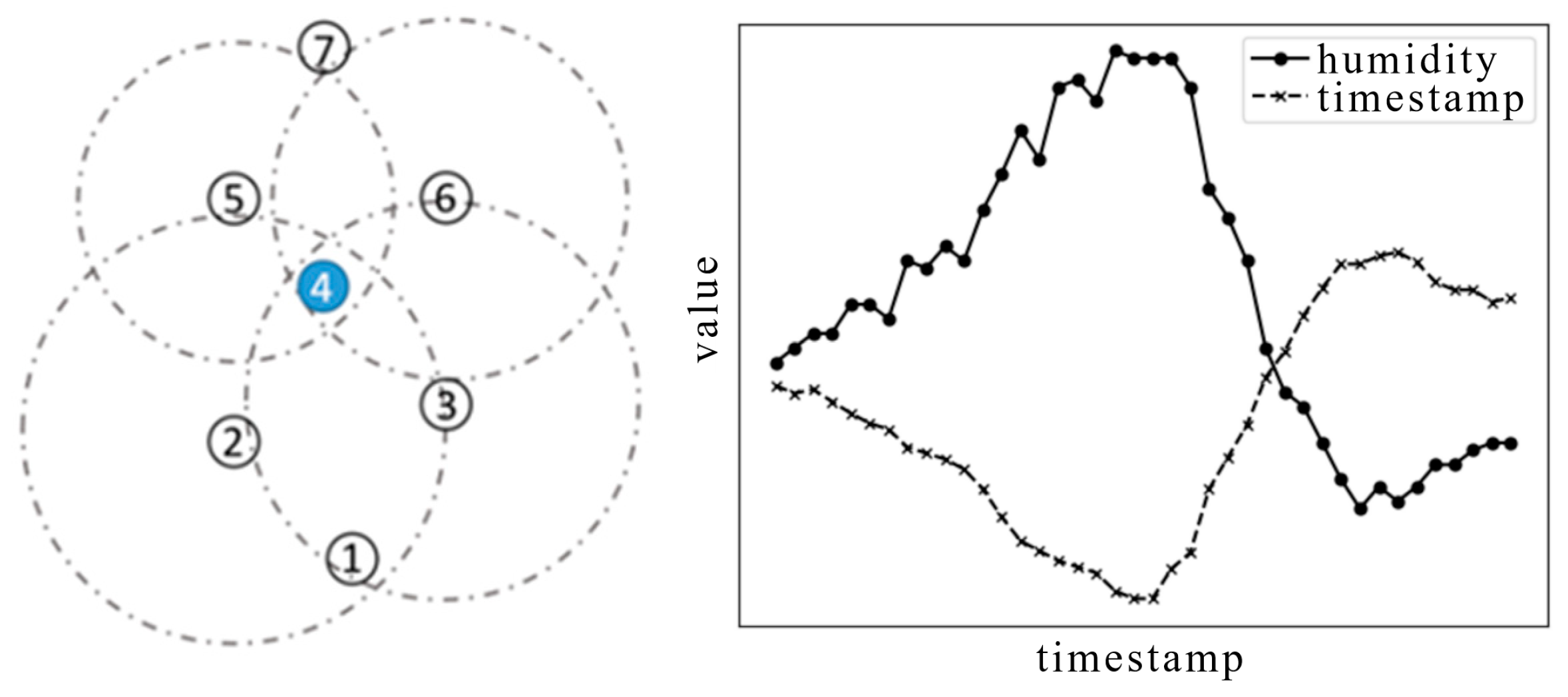
Figure 2.
Artificial neural network structure diagram.
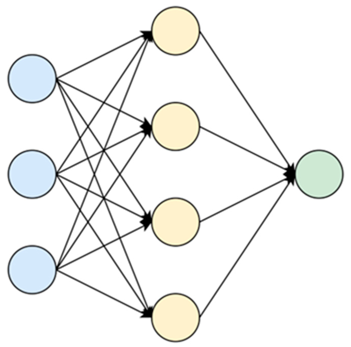
Figure 3.
Nodes of the bull attention here.
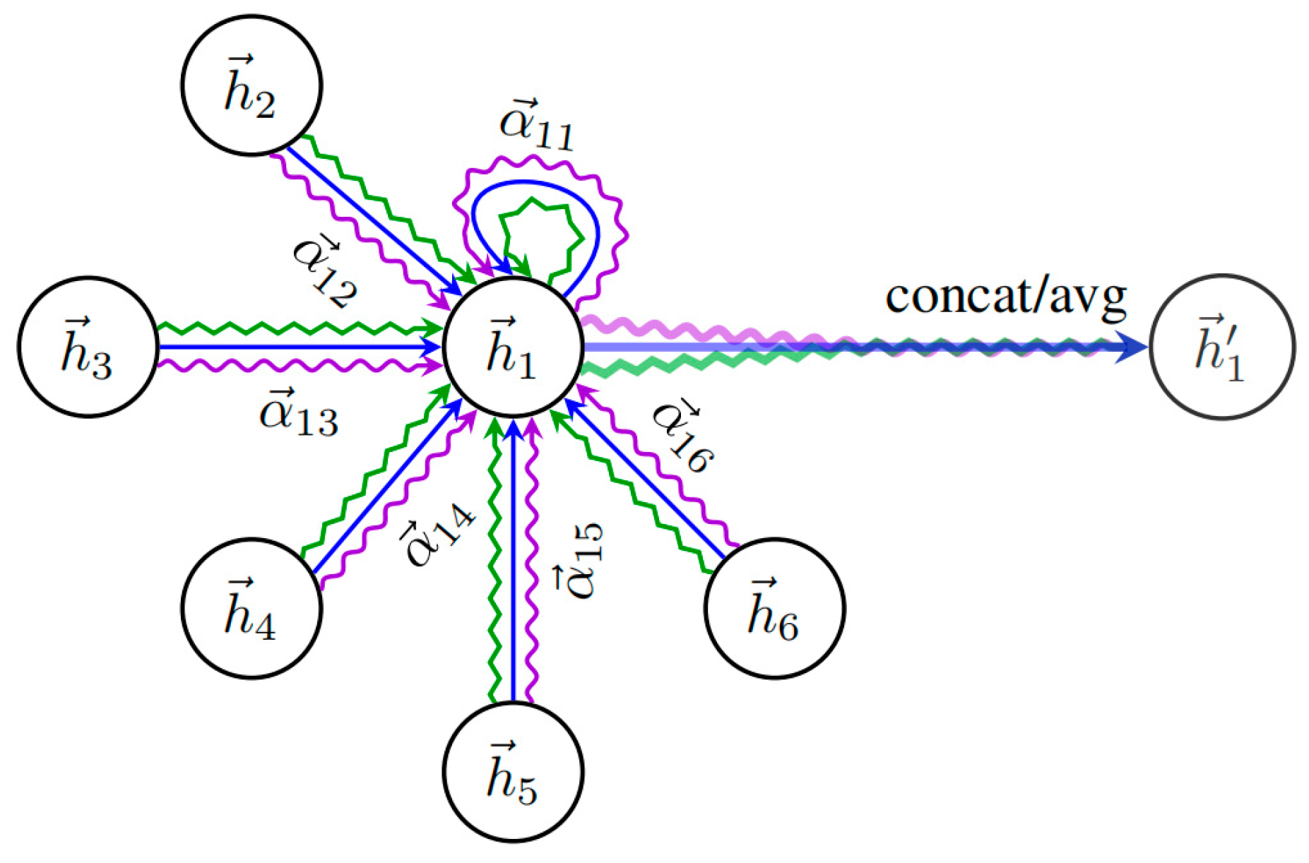
Figure 4.
ST - DMLAD model frame.
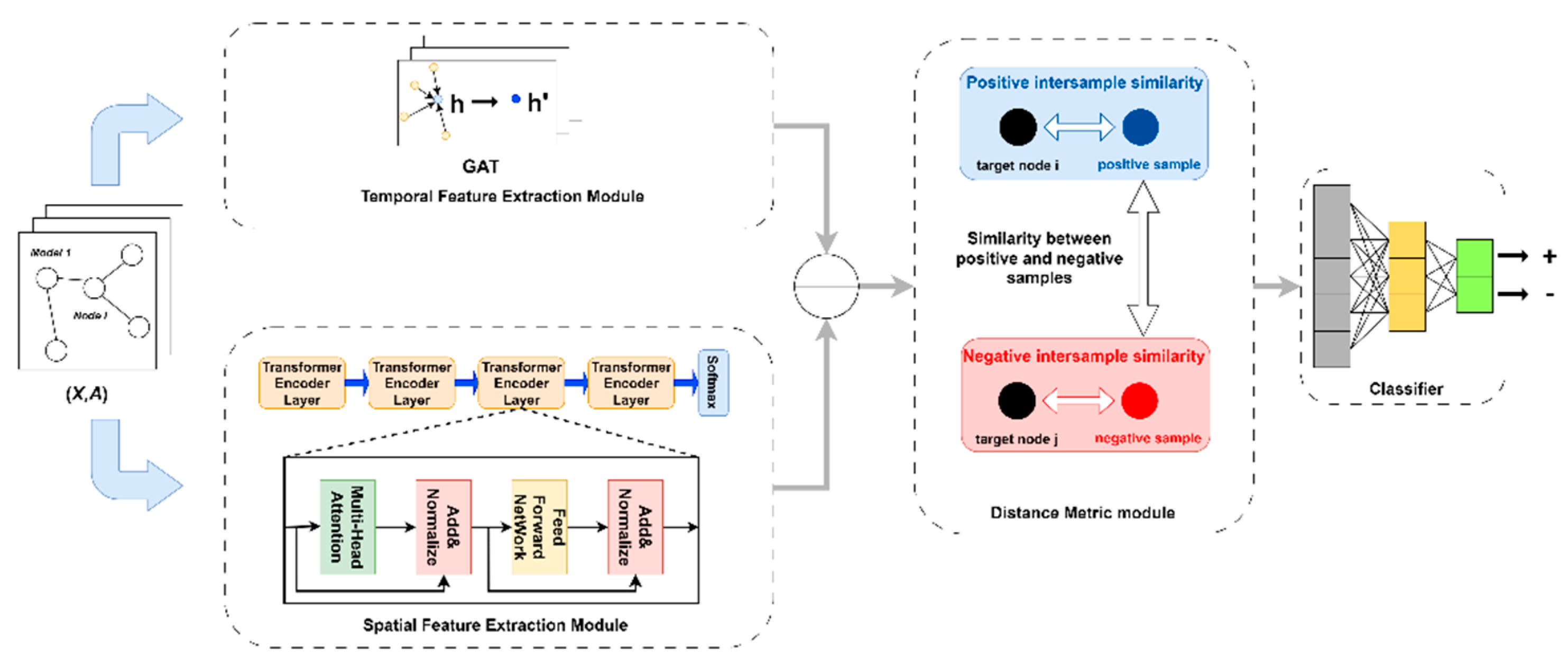
Figure 5.
Map of sensor spatial location distribution for wireless sensor network dataset collected by Intel Berkeley Lab field deployment.
Figure 5.
Map of sensor spatial location distribution for wireless sensor network dataset collected by Intel Berkeley Lab field deployment.
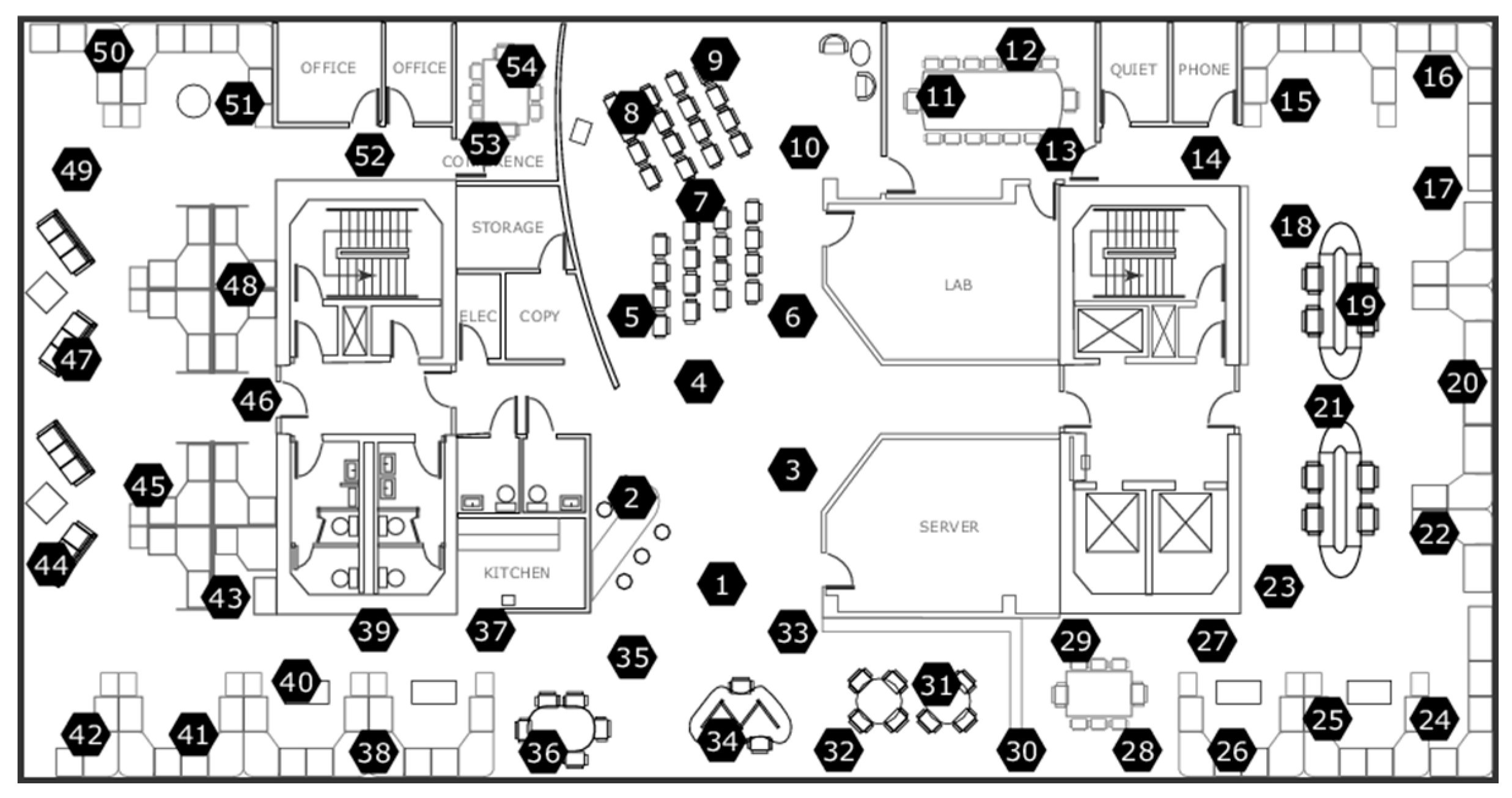
Figure 6.
Comparison figure before and after point anomaly injection.
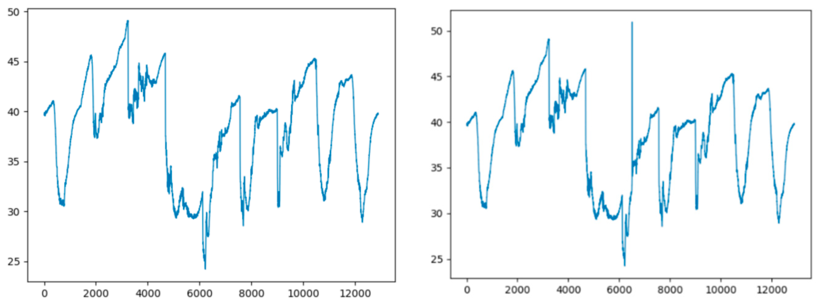
Figure 7.
Comparison before and after injecting contextual anomalies with an upward trend.
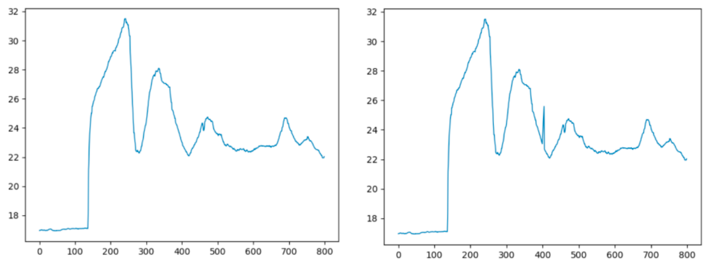
Figure 8.
Schematic of the injected collective exception.
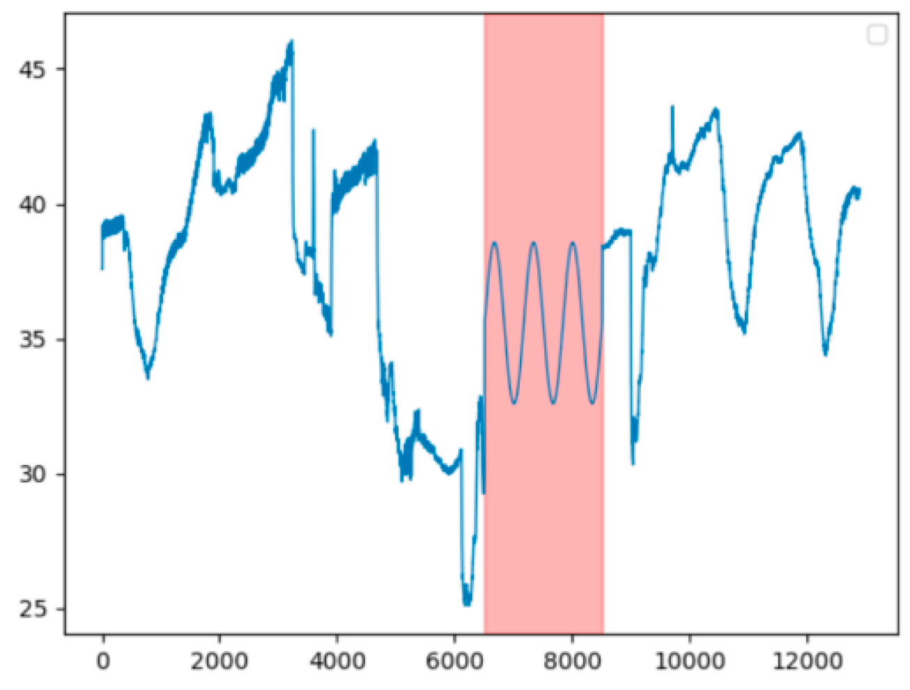
Figure 9.
Similarity score calculation module structure diagram.
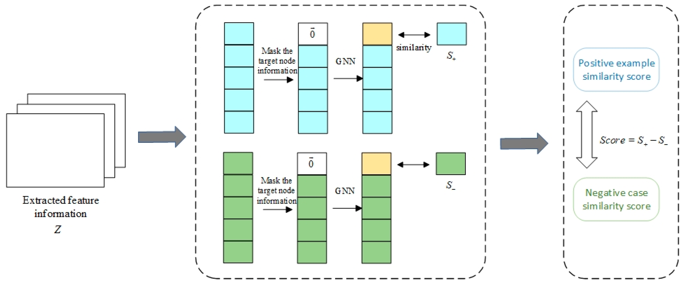

Table 1.
Module package versions.
| Module package | Version number |
|---|---|
| datashape | 0.5.4 |
| matplotlib | 3.5.2 |
| matplotlib-inline | 0.1.6 |
| numpy | 1.21.5 |
| pandas | 1.4.4 |
| pip | 22.2.2 |
| scipy | 1.9.1 |
| torch | 1.13.0 |
| torchvision | 0.14.0 |
| tqdm | 4.64.1 |
| wheel | 0.37.1 |
| zipp | 3.8.0 |
Table 2.
Ablation experiment results.
| Serial number | Feature extraction method | Similarity acquisition method | Prec | Rec | F1 | ||
| GCN | This feature extraction module | Similarity score calculation module | This design distance measurement module | ||||
| 1 | √ | √ | 0.72 | 0.53 | 0.61 | ||
| 2 | √ | √ | 0.97 | 0.76 | 0.85 | ||
| 3 | √ | √ | 0.8 | 0.83 | 0.82 | ||
| 4 | √ | √ | 0.95 | 0.84 | 0.89 | ||
Table 3.
Comparison of experimental results.
| Option | Prec | Rec | F1 |
| CNN-LSTM | 0.75 | 0.6 | 0.67 |
| GCN-LSTM | 0.79 | 0.73 | 0.76 |
| GAT-GRU | 0.89 | 0.82 | 0.85 |
| GAT-Transformer | 0.95 | 0.71 | 0.81 |
| ST-DMLAD | 0.95 | 0.84 | 0.89 |
Disclaimer/Publisher’s Note: The statements, opinions and data contained in all publications are solely those of the individual author(s) and contributor(s) and not of MDPI and/or the editor(s). MDPI and/or the editor(s) disclaim responsibility for any injury to people or property resulting from any ideas, methods, instructions or products referred to in the content. |
© 2025 by the authors. Licensee MDPI, Basel, Switzerland. This article is an open access article distributed under the terms and conditions of the Creative Commons Attribution (CC BY) license (http://creativecommons.org/licenses/by/4.0/).
Copyright: This open access article is published under a Creative Commons CC BY 4.0 license, which permit the free download, distribution, and reuse, provided that the author and preprint are cited in any reuse.


