
Submitted:
26 March 2025
Posted:
26 March 2025
You are already at the latest version
Abstract
This paper introduces a platform-level approach for aircraft data simulation, offering a holistic perspective to study system interactions and fault propagation across flight phases. Building on the earlier work on Framework for Aerospace Vehicle Reasoning (FAVER), this work integrates altitude-dependent fault propagation and cascading effects through the use of a Virtual Aircraft Model (VAM). The Virtual Aircraft Model (VAM) is developed by integrating four aircraft system models into a unified model and automating the simulation of fault scenarios across Federal Aviation Administration (FAA)-defined flight phases. A solution vector is derived to efficiently manage extensive simulation runs, incorporating various systems, fault modes, flight phases, and degradation severities. Initial results validate the model’s effectiveness in capturing both healthy states and fault propagation cases in the data generated at both the system and platform levels. Given the huge amount of data generated, the Hyper-computing Integrated Layer for Digital Aviation (HILDA), a high-performance computing system, is used to ensure efficient simulation execution. Enhancements within the VAM, including an optimised "order of run," dictate the sequence of fault mode simulations to capture cross-system interactions. By enabling this platform-level approach through the VAM, the siloed system-specific analyses is avoided, bringing the potential of integrated feedback to original equipment manufacturers (OEMs) and maintenance personnel. This work establishes a foundation for future work on State of Health (SoH) and prognostic assessment, facilitating advanced health management.
Keywords:
Platform health management
; Digital Twins
; Virtual Aircraft Model (VAM)
; Flight Profile
; Flight Phases
; Original Equipment Manufacturers (OEMs)
; Cascading Effects
; Symptom Vector
; Order of Run
; State of Health (SoH)
1. Introduction
The aviation industry is undergoing a transformation as data-driven approaches are increasingly adopted to enhance aircraft reliability and operational efficiency. Original Equipment Manufacturers (OEMs) play a pivotal role in this shift. Their advanced sensors and critical components form the backbone of modern aircraft, enabling real-time performance monitoring. These sensors, strategically distributed across various systems, generate continuous streams of flight data [1]. When analysed effectively, the vast amount of sensor data holds significant diagnostic potential, enabling improved fault detection, optimised maintenance schedules, and enhanced overall operational efficiency [2,3]. To fully leverage this data, advanced analytical frameworks are required. Digital twins have emerged as a key technology in this domain, providing virtual replicas of aircraft systems that enable real-time monitoring, predictive diagnostics, and proactive maintenance strategies.
1.1. Digital Twins
Digital Twins (DTs) have emerged as a transformative technology in various industries, particularly in aerospace, where they enhance diagnostics and predictive maintenance. A DT is more than a static model; it is a dynamic virtual replica of a physical asset, continuously updated through real-time data acquisition from sensors and other monitoring technologies. This continuous feedback enables accurate reflection of the asset's current state and prediction of its future behaviour, linking virtual model to physical asset [4]. In aviation, DTs have been widely applied in aircraft design, manufacturing, and maintenance. They facilitate condition monitoring, structural health management, and failure detection, ensuring system reliability and safety while reducing operational costs. For instance, DTs enable predictive maintenance by forecasting the remaining useful life of critical components, such as engines and hydraulic systems, thereby minimizing unplanned downtime and optimizing maintenance schedules [5]. Additionally, artificial intelligence and machine learning techniques have been integrated into DT frameworks to enhance fault detection and improve decision-making in maintenance operations [6].
One of the key contributions of DTs in aerospace is their role in Integrated Vehicle Health Management (IVHM) [7], which supports condition-based maintenance by continuously monitoring, diagnosing, and prognosing system health. DTs play a crucial role in aircraft simulations and in previous years, aerodynamic digital twins have been implemented at the platform level through the Framework for Aerospace Vehicle Reasoning (FAVER) [4]. This framework has demonstrated significant potential in managing aircraft health. Building on the foundation of FAVER, this paper advances the framework by replacing one of its digital twins and deploying it in an automated manner within a predefined mission profile.
1.2. Aircraft Simulations
Aircraft simulations are a crucial part of modern aircraft health monitoring systems, facilitating the development and validation of fault detection algorithms, failure mode analysis, and maintenance optimization. The aviation sector’s increasing reliance on these simulations reflects their critical role in enhancing operational efficiency, optimizing maintenance schedules, and reducing operational costs [8]. Simulations provide a controlled environment for testing various operational scenarios and failure modes without real-world risk, thereby allowing for the refinement of diagnostic and prognostic techniques [9]. Different types of simulations, from component-level to system-level and platform-level, play distinct roles in aircraft health monitoring research. Component-level and system-level simulations focus on individual systems and are computationally efficient for rapid testing but cannot analyse cross-system interactions. For example DTs for a turbine blade [10] or a spool valve [11]. In contrast, platform-level simulations provide a holistic view of system interactions and their combined impact on performance under various operating conditions [12]. They are particularly valuable for understanding how localized issues, such as engine degradation, propagate across other systems and impact functionality under varying operating conditions [13]. However, they may require greater computational resources and advanced modelling techniques. Platform-level simulations are less common due to the challenges of conceptualizing cross-system relationships and the complexity of modelling a unified digital twin by integrating multiple systems. Glaessgen and Stargel (2012) note that combining diverse subsystems into a single platform-level model demands advanced methodologies to manage interdependencies and ensure accurate predictions [1]. Kritzinger et al. (2018) argue that component-level digital twins are more practical, as they focus on specific subsystems like valves or sensors, simplifying modelling and reducing computational demands [2]. Additionally, Schleich et al. (2017) highlight that integrating multiple systems into a platform-level digital twin often introduces scalability issues and uncertainties, making it harder to achieve the accuracy and reliability of component-level models [3]. To address these gaps and demonstrate the usefulness of platform level simulation, this paper introduces the Virtual Aircraft Model (VAM), a platform-level simulation that integrates four key aircraft systems—Engine (ENG), Fuel System (FS), Environmental Control System (ECS), and Electrical Power System (EPS)—into a unified model.
The VAM simulates the interconnected behaviours of the aircraft systems under varying flight conditions and operational scenarios. This comprehensive approach ensures that faults and component degradation propagate across systems and operating conditions, allowing for a detailed analysis of how localized faults trigger cascading effects throughout the aircraft. Highlighted in Figure 1 is the relationship between the VAM, DTs and fault diagnosis.
This paper is organized into six sections, including the present one. Section 2 discusses the key aspects of the FAVER framework, specifically the role of Digital Twins in FAVER, including the replacement of the FS simulation and the associated inputs and data outputs. Section 3 explores the development of the Virtual Aircraft Model (VAM), detailing the process of selecting aircraft routes and FAA-defined flight phases. This section also discusses how the flight profile is integrated within the VAM, ensuring a realistic and structured approach to analysing aircraft performance. The fourth section delves into the extensions made to the FAVER framework, with a particular focus on the tailored workflows developed for running the VAM. These enhancements facilitate streamlined integration and improved simulation efficiency within the VAM. Section 5 presents the simulation setup for the VAM and examines the adoption of HILDA for executing the simulations. This section outlines the reasoning behind the use of HILDA, detailing its advantages in efficient simulations and data-driven analysis. The sixth section highlights the capability of the VAM and the initial results for state of health detection. Finally, the seventh section provides a conclusion and discussion, summarizing the key findings and initial results from running simulations with the VAM, and the foundation it lays for further work in state of health (SoH) detection and health index prognosis.
2. Digital Twins
Digital twins lie at the heart of FAVER [4], Figure 1, which provides system-level diagnostics for the detection and analysis of aircraft faults by leveraging digital twins of key systems, including ENG [14], EPS [15] and ECS [16]. For each system ‘virtual’ sensors provide the data, the system symptom vector (SSV), on which the diagnostics operate. When these sensor signals are combined at the platform level the result is a platform symptom vector (PSV). FAVER further incorporates data-in-the-loop for the FS [17] and a reasoning layer designed to identify faults, trace their origins, and evaluate potential cascading effects of component faults, based on the PSV. Every system is modelled to simulate both normal and faulty conditions. According to the literature it is the only one of its kind.
The EPS digital twin is designed to replicate the behaviour of an aircraft's electrical power system. It features a constant-speed power source derived from the engine shaft, which drives a 40 kVA generator [15]. Its generator is modelled as a simplified synchronous unit within MATLAB Simulink, producing 115/200V AC power at a nominal frequency of 400 Hz [15]. Operating at a constant speed of 12,000 rpm, as determined by the system’s design parameters, the synchronous machine ensures stable voltage levels and accurately simulates real-world scenarios. Additionally, the EPS digital twin is equipped with a regulated field voltage input, managed by a voltage regulator with an integrated excitation system to maintain consistent performance.
The Environmental Control System (ECS) is simulated using the Simscape Environmental Control System Simulation under All Conditions (SESAC) framework [16]. Configured to simulate the B737-800 Passenger Air Conditioner (PACK), the model has been validated against actual aircraft data, ensuring accuracy. It replicates ECS operation under both healthy and faulty conditions.
The engine is an open-source model of the Pratt & Whitney JT9D high-bypass turbofan, implemented as a digital twin using T-MATS, a MATLAB Simulink-based simulation platform [14]. Designed to represent a typical high-bypass turbofan engine, it features a bypass ratio of 4.8:1, a one-stage fan, a three-stage low-pressure compressor (LPC), and an 11-stage high-pressure compressor (HPC). The engine includes an annular combustion chamber, a two-stage high-pressure turbine (HPT), a four-stage low-pressure turbine (LPT), and a convergent-divergent nozzle.
Each aircraft system comes with its own possible fault modes, as shown in Table 1. Further, each fault mode comes with its own degradation severity (DS) expressing how far the degradation has progresses. For example, DS=0 is a healthy case and a DS=0.5 expresses a significantly degraded case. Most of these cases have come from industrial experts, signifying the most likely faults for that system. Additionally, the data-in-the-loop for the FS, has been replaced with a fuel system simulation DT as discussed below.
2.1. Fuel System Simulation
In this work the FS data-in-the-loop from previous work has been replaced with a simulation model which runs to supply fuel to the ENG at the desired flow rate. The model is designed to replicate the pressure and flow of fuel in an aircraft fuel system, and was developed using the pressure and flow characteristics derived from the pump and Direct Proportional Valves (DPVs) of a closed-loop fuel rig at the IVHM Centre, Cranfield University, UK, shown in Figure 2. The rig comprises:
- Reservoir: Supplies fuel (represented by water in this setup).
- Pump: Motor-driven, equipped with an internal relief valve.
- Valves: Control fuel flow.
- Filter: Removes contaminants.
- Flowmeters: Monitors fuel flow.
- Nozzle: Regulates outlet fuel flow.
2.1.1. Inputs for Fuel System Simulation
- Pump Characteristics: Flow and pressure ratio correlations, obtained from the fuel rig experiments. The simulation is set to run at a constant speed of 400 rpm.
- DPV Characteristics: Flow and pressure drop correlations, obtained from the fuel rig experiments.
- Initial Flow Input: The initial flow input to set the baseline state of the system.
- Bernoulli’s Equation: Bernoulli’s equation calculates flow rates within the system.
2.1.2. Fuel System Data Output
The FS produces two types of data:
- Pressure data (P1–P9): Measurements captured at strategically placed sensors to monitor system pressures.
- Flow: Records the flow rate within the system.
2.2. Symptom Vectors
Symptom vectors serve as distinctive signatures that characterize both healthy and faulty system states. As illustrated in Table 2, each system is represented by its own System Symptom Vector (SSV), indicated by the tick marks. The SSV consists of features and operating conditions derived from the simulations. These features capture the performance of each system and specific operating conditions which characterise the runs.
The Platform Symptom Vector (PSV) is a collection of the SSVs from all the systems. including data on cascading macro effects, which are captured through system interactions. Each system either passes a percentage of its output;100% when in a healthy state and a reduced value when degraded, or provides an expected feature value as an input for the next system in the sequence. This mechanism ensures that cascading effects are represented within the PSV. For instance, the FS supplies fuel flow to the ENG. If the fuel system has no degradation that affects fuel flow, it delivers 100% of the expected fuel flow to the engine. However, when degradation occurs, leading to reduced fuel flow, only a lesser percentage reaches the engine. This reduction may, in turn, affect the shaft power generated by the engine. Thus, the ENG would pass a reduced value for reduced shaft power to the EPS. By combining the SSV from local systems along with their interactions, PSV enables the behaviour of macro effects propagated through interconnected systems.
3. Development of the VAM
The Virtual Aircraft Model (VAM) provides a comprehensive framework for simulating both normal and degraded scenarios of aircraft components across various flight phases. By integrating digital twins that accurately replicate the EPS, FS, ENG, and ECS, the VAM enables platform-level data generation while accounting for operating conditions and system interactions. This integration is established based on the interdependencies between these systems, as illustrated in Figure 1.
When the EPS supplies power to all the systems, each system checks to see if the required electric current has been supplied by comparing the required to the supplied. In the same manner, when the FS supplies fuel flow to the ENG, the ENG receives it as a percentage of the total required fuel flow; 100% when it supplies all the needed flow and a lesser percentage when it doesn't. In turn, the Engine generates shaft power to drive the EPS, enabling electrical power generation. The EPS checks this by comparing the required rpm to the supplied rpm. Additionally, when the Engine supplies bleed air to the ECS, the ECS compares the supplied pressure and temperature to the required pressure and temperature to check for any difference, indicating a cascaded fault.
A key advantage of the VAM is its ability to model system-wide fault progression, offering insights into how failures propagate across interconnected systems [9]. For example, it can simulate a fuel system malfunction affecting engine performance, which subsequently impacts electrical power output, providing a holistic view of cascading failures. The VAM produces vast amounts of data, which is fed into a unified repository (data lake). This data lake serves as a resource for training and validating machine learning-based diagnostic and prognostic algorithms, eliminating the need for extensive external data fusion [18].
To comprehensively model faults and their interactions, ensuring that simulation-generated data accurately captures the effects of system behaviour, fault modes, degradation severity, and flight phases under various operating conditions, this work employs a structured approach using a solution vector (SV) which is defined by:
where:
SVi,j,k,l
‘i’ represents the flight phase being analysed.
‘j’ denotes the fault type or fault mode.
‘k’ is the set degradation severity of the fault.
‘l’ corresponds to the order of run for the fault mode.
Each parameter within this SV is bounded by specific limits, defining the complexity and scale of the analysis, as highlighted in Table 3.
Using the solution vector, the VAM provides the flexibility to execute targeted simulations, allowing for the analysis of a specific system or a combination of systems under desired flight phases, particular degradation levels, and specific operating conditions. This adaptability enables focused investigations into critical failure scenarios, facilitating precise diagnostics and performance assessments without requiring exhaustive full-scale simulations.
3.1. Aircraft Route Selection and Definition of Flight Phases
With the virtual aircraft and its operating conditions now defined, the next step is to select the routes for its flight and identify the flight phases to be monitored during the simulation of the fault scenarios under consideration. The flight phases, derived from the flight profile for the chosen routes represents a range of conditions under which the aircraft operates, including variations in altitude, Mach number, and thrust demand.
Flight data is essential for simulating virtual aircraft models, as it allows for the modelling of flight dynamics and operational conditions, as evidenced in [19,20,21]. This work uses a web-based tool designed in [22] for generating flight data. This tool leverages advanced computational techniques to produces flight data. It integrates computational models and visualization features, offering 4D trajectory computation, customizable inputs, and real-time environmental integration. Key inputs include aircraft specifications, flight conditions, and route details, while incorporating real-time weather data from sources like Meteorological Aerodrome Report (METAR) and National Oceanic and Atmospheric Administration (NOAA) to enhance accuracy.

Table 4.
FAA flight phase definition.
| Phase | Definition | Parameters/Conditions |
| Taxi | Ground movement of the aircraft before takeoff or after landing. Altitude is at ground level, Mach number is 0, and minimal thrust is required. | Taxi speeds are maintained below 20 knots. Pilots ensure proper control with braking and steering to follow taxiways and avoid obstacles. |
| Takeoff | From the application of takeoff power until reaching an altitude of at least 50 feet above the surface or obstacle clearance. Mach number is low (around 0.1–0.2) and thrust is set to maximum takeoff power. | Parameters include maintaining VX (best angle of climb speed) initially and transitioning to VY (best rate) after obstacle clearance. Ensure a positive rate of climb before retracting gear. |
| Climb | Begins immediately after takeoff until reaching cruise altitude (typically 25,000–40,000 feet). Mach number increases gradually, and thrust demand is reduced to climb power settings. | En route climb speed (higher than VY) is maintained. Power settings and engine cooling are optimized as per POH/AFM. Gradual adjustments in pitch and trim ensure stability. |
| Cruise | Level flight phase maintained until the descent begins. Altitude is constant (typically 30,000–40,000 feet), Mach number is steady (0.78–0.84 for jet aircraft), and thrust demand is minimal for steady speed. | Cruise power and rpm are set based on the performance tables in the POH/AFM. Mixture leaning and fuel management are monitored for efficiency. |
| Top of Descent (TOD) | The point where descent begins to meet planned altitude and speed constraints at destination. Mach number decreases gradually as altitude reduces from cruise levels, and thrust demand is set for descent. | TOD is calculated using descent profile, planned descent rates, and distance. Wind, terrain, and air traffic control (ATC) factors are considered. |
| Descent | Reducing altitude towards the destination or next waypoint. Altitude decreases to final approach level (e.g., 3,000–5,000 feet). Mach number continues decreasing (e.g., 0.5–0.7), and thrust demand is minimal. | Typical descent rates are 500–1,000 fpm. Adjustments for speed, drag, and energy management maintain controlled descents. Different descent profiles may apply based on requirements (e.g., cruise descent, obstacle clearance). |
The flight phase definitions provided in Table 2, derived from the Federal Aviation Administration (FAA) and closely aligned with the descriptions in [23], served as the basis for selecting key points from the chosen flight profile for simulations with the VAM. Each phase is characterized by distinct operational conditions, including altitude, Mach number, and thrust demand.
3.2. Integrating the Flight Profile with the VAM
The chosen flight profile, depicted in Figure 4, was generated using the input configuration of an Airbus A320 with a take-off mass of 64,000 kg from [22]. The requested flight level was 41,000 feet. The route selected was from Atlanta-Hartsfield Jackson International (ATL) to Los Angeles International (LAX). The generated flight path in Figure 4 shows the corresponding flight trajectory based on these inputs, highlighting key flight phases along the route, including taxi (1), take-off (2), climb (3), cruise (4), top of descent (5), and descent (6) phases (from Table 2). Each phase was intentionally selected to provide a distinct representation of the aircraft’s operational behaviour throughout the journey.
By integrating the flight phases with the VAM, the model is able to simulate fault modes while accounting for the unique operational dynamics of each phase. The VAM leverages critical parameters, such as altitude, Mach number, and thrust demand, to generate data. However, only the Engine and Environmental Control System (ECS) are designed to adapt dynamically to these inputs due to their direct dependency on flight-phase conditions. In contrast, the FS and EPS are modelled independently of flight phases. This decision is based solely on an engineering assumption by the authors, wherein FS and EPS are considered to supply fuel and power continuously, with their performance only affected by the presence of faults rather than variations in flight phases. The Engine within the VAM adjusts its performance based on inputs related to altitude and Mach number. For example, during take-off, the engine operates at maximum thrust to provide sufficient acceleration and lift, accommodating the rapid increase in speed and altitude. In cruise, it stabilizes thrust to maintain efficiency while counteracting drag and other aerodynamic forces at typical cruising altitudes between 30,000 and 40,000 feet and speeds ranging from Mach 0.78 to 0.84. This aligns with findings from [24,25], which emphasize the importance of accurate thrust modulation in maintaining operational efficiency during different flight phases. Similarly, the ECS dynamically manages cabin conditions based on changing altitudes. During the climb phase, it compensates for decreasing external air pressure by gradually increasing cabin pressure, maintaining structural integrity and ensuring passenger comfort, which is equivalent to conditions experienced at altitudes up to 8,000 feet. Conversely, during descent, the ECS carefully manages pressure transitions to prevent sudden changes that could cause discomfort or mechanical stress. As highlighted by [26], effective ECS adjustments during altitude changes are vital to maintaining safe and stable cabin environments. Unlike the ENG and ECS, the FS and EPS are modelled without dynamic adjustments to flight-phase parameters, although fault simulations in them are able to send cascading effects to the systems they affect. The FS operates with predefined flow rates that correspond to engine demands, remaining consistent regardless of changes in altitude or Mach number, but for a fault. Similarly, the EPS operates under baseline or scenario-specific loads without modifying its behaviour based on flight conditions, except the introduction of a fault [15].
Table 5.
System behaviour across flight phases.
| Flight Phase | ENG | ECS | FS | EPS |
| Taxi | Operates at low thrust for ground movement. | Maintains cabin pressure and temperature at ground-level conditions. | Provides fuel flow at a set rpm | Supplies power at varied loads for systems. |
| Take-off | Operates at maximum thrust for acceleration and lift. | Adjusts cabin pressure to compensate for rapid altitude increase. | Provides fuel flow at a set rpm | Supplies power at varied loads for systems. |
| Climb | Adjusts thrust to balance climb rate and efficiency. | Gradually increases cabin pressure to match decreasing external pressure (up to 8,000 ft equivalent). | Provides fuel flow at a set rpm | Supplies power at varied loads for systems. |
| Cruise | Stabilizes thrust for efficiency at 30,000–40,000 ft and Mach 0.78–0.84. | Maintains stable cabin pressure and temperature at cruising altitude. | Provides fuel flow at a set rpm | Supplies power at varied loads for systems. |
| Top of Descent | Reduces thrust as the aircraft prepares to descend. | Prepares for pressure adjustments during descent. | Provides fuel flow at a set rpm | Supplies power at varied loads for systems. |
| Descent | Further reduces thrust to manage descent rate. | Carefully manages cabin pressure transitions to prevent discomfort or mechanical stress. | Provides fuel flow at a set rpm | Supplies power at varied loads for systems. |
This simplification follows the recommendations of [27], which advocate reducing model complexity for systems that are less sensitive to operational variability. The selective integration of flight-phase-specific dynamics enhances the operational fidelity of the VAM while maintaining computational efficiency. The ENG and ECS provide realistic responses to changing operational inputs, allowing for detailed fault simulations. For example, an engine fault during the climb phase can be modelled with precise adjustments to thrust demand and altitude, while potential cascading effects on the EPS can still be assessed under consistent baseline conditions. This approach reflects findings in the literature [28,29], which highlight the importance of system-specific dependencies in improving fault diagnostics. The integration of flight phases enables comprehensive, scenario-based fault analysis across multiple flight conditions. For instance, faults in the ECS during descent can be analysed in the context of cabin pressure degradation, while engine performance during take-off or cruise can be modelled with high accuracy. This phase-aware approach is consistent with recommendations from [30], which emphasize the importance of phase-specific modelling for effective diagnostics. By focusing on the Engine and ECS for flight-phase-specific adaptations, the VAM achieves a balance between operational fidelity and modelling simplicity. As a result, the VAM is well-suited for generating reliable data for fault diagnostics and safety evaluations across diverse operational scenarios.
4. Tailored Workflows for The VAM
The FAVER framework has been extended in this work to enhance data generation and facilitate more comprehensive diagnostic analysis. These developments, depicted in Figure 5 (highlighted in yellow), include key advancements such as the replacement of the FS shown in Figure 2 with a simulation model.
One of the extensions that the VAM introduces is an automated structured “order of run” for fault mode simulations, illustrated in Figure 6. This “order of run” establishes a standardized sequence for simulating the 25 considered fault modes, ensuring that the final data output captures the cumulative and cascading effects of faults across interconnected systems. The logic underlying this sequence was developed based on engineering judgment and feedback from industrial partners. For example, consider FM8 in the FS. The FS is run first to determine the impact of the failure on the fuel flow. Next, the ENG is run to propagate the effect of a reduced fuel flow into the engine, influencing parameters such as thrust output. Since the engine supplies shaft power to the EPS, the EPS is run subsequently to account for reduced power availability. Finally, because the EPS provides power to the ECS, the ECS is run last to propagate any resulting effects from the EPS.
As emphasized in the literature, capturing cascading failures and the interactions between systems is critical for developing multi-system diagnostic frameworks [31]. To implement this structured order of simulation, each system within the VAM was assigned a unique identifier to reflect its role and interdependencies as shown by the system in Figure 7. In addition to the structured fault simulations, another critical extension involves the generation of platform-level data. This data combines system outputs, cascading effects, flight phase information, and degradation severity related to specific fault modes into a comprehensive dataset. The resulting platform data is well-suited for analysing aircraft health under diverse operational conditions, thereby supporting data-driven diagnostics and prognostics.
5. Simulation Setup and HILDA Adoption
The simulation setup is structured according to the run sequence outlined in Figure 7, which follows the defined SV. This setup allows for the selection of specific operational conditions, including flight phase, fault mode, and degradation severity level. For each selected fault mode, the simulation adheres to a predefined order of run, illustrated in Figure 6. The flexibility of this framework allows for scaling the number of simulation runs by increasing the number of any of the variables within SVi,j,k,l. For example, the number of altitudes can be expanded, additional fault modes can be introduced, or the range of degradation severity variations can be increased. In this work, the authors chose to expand the degradation severity variations to generate a larger dataset for analysis. The total number of platform data incidents is determined using the following equation:
Equation 1 provides insight into generating data across diverse scenarios. Depending on the number of data incidents required, the equation serves as a guide for selecting which variables to perturb, ensuring a balanced and representative dataset. By capturing all possible combinations of system faults and their severities, it strengthens the robustness of analysis, leading to more accurate predictions and deeper insights into system performance and failure trends. As a rule of thumb, a minimum of 200 data incidents are required for each scenario defined by the equation to ensure statistical significance and robust analysis [32]. Keeping all the variables in equation fixed except ‘k’, the minimum generated data will include about 60 different variations of ‘k’ per scenario, resulting in a total of 9,000 data incidents. Where an increased number of ‘k’ is required, say 10 times the initial value (600), the total data incidents would scale accordingly, reaching 90,000. Specifically, this would comprise 25,200 data incidents each for EPS and ENG fault modes, 21,600 for FS fault modes, and 18,000 for ECS fault modes. This structured approach ensures a systematic method for scaling data generation based on variations in system configurations or fault scenarios.
Figure 8.
Run sequence for the VAM.

The extensive computational demands of simulating such a large number of fault scenarios necessitated the use of the Hypercomputing Integrated Layer for Digital Aviation (HILDA), housed at Cranfield University, UK. HILDA is a high-performance computing environment specifically designed for large-scale simulations, offering 10.2 petaflops of computational power, 2.7 petabytes of local data storage, and advanced GPU rendering capabilities. HILDA’s architecture integrates multi-core processors, extensive RAM, high-speed storage, and advanced GPU capabilities, enabling the rapid processing of large datasets. Designed for high-performance computing, its infrastructure supports complex, data-driven diagnostics by ensuring optimal resource allocation and parallel execution of simulations. By leveraging its secure and scalable environment, the framework achieves faster simulation runtimes.
Figure 9.
Comparison of HILDA's Specs vs Allocated VM Resources.
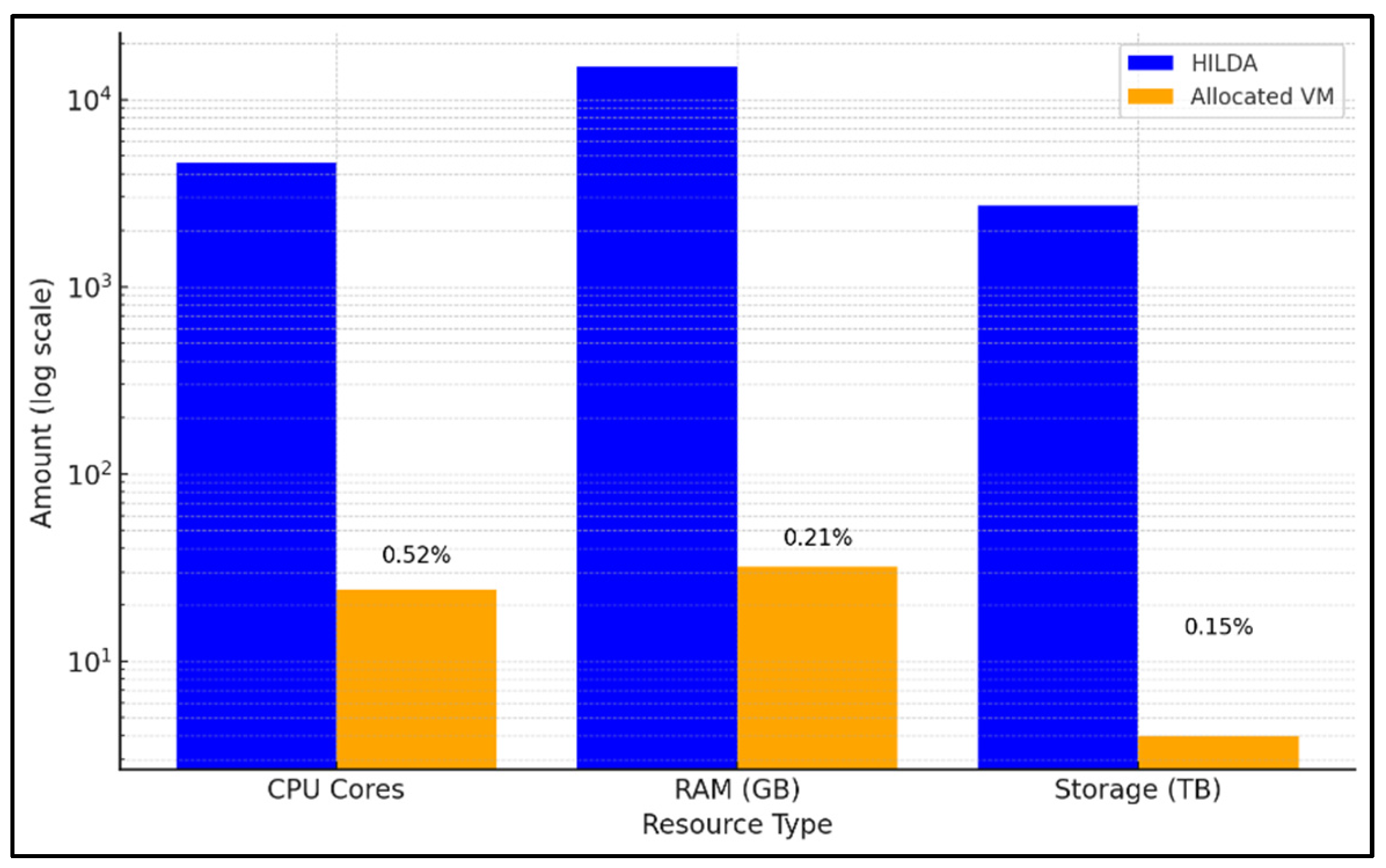
HILDA features a 4,576-core CPU cluster, 110,592 compute GPU CUDA cores, 41,472 rendering GPU CUDA cores, 15TB RAM, 2.7PB encrypted storage, and a 200Gb IB HDR fibre network. A virtual machine (VM) with 2 × NVIDIA GPU A4000, 24 CPU cores, 32GB RAM, and 4TB storage was allocated for simulations. This represents approximately 0.52% of CPU cores, 0.21% of RAM, and 0.15% of storage from HILDA. Increasing resource allocation would further improve processing speed and efficiency. HILDA’s parallel processing reduces simulation runtimes significantly. From Equation 1, a test platform run with i = 4, j = 1, k = 1, and l = 1 on a standard personal computer with an Intel Core i7-10510U took nearly five times longer than on HILDA’s VM. While the current allocation already enhances performance, more resources would optimize fault propagation modelling and high-fidelity simulations even further. This significant improvement underscores HILDA’s efficiency in handling the intensive computational demands of fault propagation modelling.
The VAM operates in two primary modes: system runs and platform runs. System runs focus on generating data from simulating fault modes within individual systems independently, without considering interactions with other systems. For each standalone simulation, a specific fault mode and degradation severity level are defined, and the simulation outputs data reflecting the performance of the selected system under that fault condition. As shown in Figure 10, the system run is configured by specifying operational conditions, beginning with the selection of one or more altitudes between 0 and 41,000 feet, demonstrating the flexibility to analyse individual phases or the entire flight profile. A specific system—EPS, FS, ENG, or ECS—is then chosen for analysis, followed by the selection of a degradation severity level to represent varying fault intensities. Once these conditions are set, the simulation executes the selected fault mode within the designated system, generating a SSV data, as illustrated in Table 2, on system behaviour while operating in isolation, without accounting for interactions with other systems.
In contrast, platform runs generate comprehensive data (PSVs) by simulating interactions and cascading effects across interconnected systems. As shown in Figure 10, the platform run is configured by specifying operational conditions, beginning with the selection of one or more altitudes between 0 and 41,000 feet, demonstrating the flexibility to analyse individual phases or the entire flight profile, followed by a specific fault mode within a system, and a degradation severity level. The chosen fault mode is then mapped to a predefined "order of run" (Figure 6), which dictates the sequence in which systems are simulated. In a platform run, all the systems are executed sequentially, ensuring a holistic representation of interactions, as opposed to system runs where only one system is run. For example, a fault mode affecting the EPS, such as FM2, triggers the simulation of the EPS first, followed by the FS, ENG, and then ECS, in accordance with the order of run in Figure 6.
6. Initial Results
The Virtual Aircraft Model (VAM) offers a range of engineering and State of Health (SoH) detection benefits. Its ability to generate comprehensive platform-level data, its flexible system configuration, its adaptability in flight phase data generation, and its capability to simulate mixed-health scenarios all contribute to its effectiveness as a diagnostic and predictive maintenance tool. The validation of Platform Symptom Vectors (PSVs) for SoH detection further highlights its potential to transform aircraft health management by enabling platform-level diagnostics.
A key feature of the VAM is its ability to generate detailed aircraft data sensed at the platform level, providing a holistic view of system interactions. The model is also designed to be flexible in the number of systems that can be incorporated into its framework. It allows additional aircraft systems to be integrated as needed, making it highly scalable and adaptable to different aircraft configurations and operational requirements. While the setup includes DTs of the EPS, FS, ENG, and ECS, the model can easily accommodate additional DTs without requiring extensive modifications. Also, the VAM can embed any flight path profiles, enabling the simulation of real-life scenarios. This ensures that the VAM remains relevant across various aircraft models and applications, making it an effective tool for both research and industry.
Another significant advantage of the VAM is its ability to generate data for specific portions of a flight phase, enabling targeted analyses. This capability allows users, particularly maintainers, to conduct focused investigations. For example, if an analysis requires a detailed examination of the take-off phase or a particular altitude, the VAM can be configured to generate data specifically for that segment. Similarly, if fault detection needs to be assessed during cruise under varying environmental conditions, the model can be adjusted accordingly. This flexibility ensures that health monitoring algorithms can be fine-tuned based on real-world operational demands, improving diagnostic accuracy and effectiveness.
Additionally, the VAM facilitates the simulation of scenarios where some systems remain healthy while others are subjected to specific fault conditions. This functionality is crucial for evaluating how interdependent systems behave under mixed-health conditions, providing a more realistic representation of real-world aircraft operations. By selectively introducing faults into certain systems while maintaining others in a nominal state, engineers can assess how failures propagate across the aircraft platform. This allows for the validation of diagnostic algorithms under complex failure modes, ensuring that fault detection techniques remain robust even when multiple systems interact.
Results from data generated by the VAM demonstrate that SoH detection, including fault classification and severity determination, can be effectively performed at the platform level using PSVs, just as it would have been done at the system level using System Symptom Vectors (SSVs). To validate this, SoH analyses were conducted at both system-level, using SSVs (A) and platform-level, using PSVs (B), comparing the results to evaluate the efficacy of using PSVs for fault detection and degradation severity prediction.
The data was generated by running the VAM across the selected route, as described in Section 3.2, and for various flight phases, including taxi, take-off, climb, cruise, top of descent, and descent. It is important to note that data from multiple flight phases, each with distinct health states, were used in this analysis. This ensures that the approach remains robust under varying operational conditions, reinforcing the reliability of platform-level SoH detection using PSVs. The dataset sizes for each system were as follows: 2160 for the EPS, 2125 for the FS, 1470 for the ENG, and 2550 for the ECS. The results from the analysis, shown in Figure 11, reveal that models trained with PSVs perform comparably to those trained with SSVs. For instance, in the EPS, Narrow Neural Network (NN) models achieved high accuracy, with Model A (SSV) at 96.8% validation and 97.6% test accuracy, and Model B (PSV) at 97.4% and 98.5%. Similarly, in the Fuel System, Narrow NN models trained with PSVs achieved near-perfect accuracy, with Model B at 99.6% validation and 100% test accuracy, closely matching the performance of SSV-trained models. These findings suggest that the VAM can effectively detect fault modes and predict their degradation severity at the platform level, leveraging PSVs and eliminating the need for system-specific diagnostics.
7. Conclusion
The Virtual Aircraft Model (VAM) has a potential to be a critical enabler of advanced fault diagnostics and health monitoring in modern aviation. VAM leverages the power of digital twins, and high-speed computer HILDA, to simulate both individual systems and platform-level interactions under diverse operational conditions, for generating a dynamic dataset for analysing fault scenarios. System interactions pose significant challenges for fault detection, and virtual models like the VAM, which is used for platform runs, offer a promising solution. The VAM’s ability to simulate various flight phases, operational conditions, and both short-haul and long-haul routes distinguishes it as a robust, integrated data-generation tool for mission-specific analysis. This allows for a deeper understanding of how operational variations impact aircraft health. For instance, an ECS with a degraded heat exchanger may perform adequately on short-haul flights but could present significant risks on long-haul, high-altitude missions due to increased environmental demands.
The VAM can interface with ground maintenance teams to pre-emptively schedule repairs, minimizing downtime and improving fleet management. Additionally, it can be integrated with real-time flight monitoring systems, functioning as a health management co-pilot that continuously tracks SVs during flight. By providing real-time feedback on component health, it enables early detection of potential issues during critical phases, allowing for timely corrective actions. While designed to analyse single faults and their cascading effects, the VAM also provides a foundation for evaluating parallel fault scenarios. This capability offers deeper insights into system resilience and cascading failure effects.
Aircraft maintenance relies on assessing the State of Health (SoH) and predicting Health Indexes (HIs) to ensure timely maintenance and operational efficiency. While OEMs (Original Equipment Manufacturers) can access platform-level data, they may lack visibility into the specific diagnostics of individual systems, making it difficult to detect faults and degradation severity at the platform. Developing a system capable of processing platform-level data and translating it into actionable insights can enable Boeing to bridge the gap between platform monitoring and siloed system monitoring, enabling more effective maintenance strategies and operational decision-making. The Virtual Aircraft Model (VAM) provides a robust foundation for advancing State of Health (SoH) assessments and Health Index (HI) developments.
References
- M. J. Scott, W. J. C. Verhagen, M. T. Bieber, and P. Marzocca, “A Systematic Literature Review of Predictive Maintenance for Defence Fixed-Wing Aircraft Sustainment and Operations,” Sensors 2022, Vol. 22, Page 7070, vol. 22, no. 18, p. 7070, Sep. 2022, doi: 10.3390/S22187070.
- S. Khalid et al., “A Comprehensive Review of Emerging Trends in Aircraft Structural Prognostics and Health Management,” Mathematics 2023, Vol. 11, Page 3837, vol. 11, no. 18, p. 3837, Sep. 2023, doi: 10.3390/MATH11183837.
- C. Wang, D. Puigh, A. Lei, W. Guo, J. Yuan, and M. Mazarek, “Lessons Learned from Aircraft Component Failure Prediction using Full Flight Sensor Data,” PHM Society Asia-Pacific Conference, vol. 4, no. 1, Sep. 2023, doi: 10.36001/PHMAP.2023.V4I1.3684.
- C. M. Ezhilarasu and I. K. Jennions, “ Development and Implementation of a F ramework for A erospace Ve hicle R easoning (FAVER) ,” IEEE Access, vol. 9, pp. 108028–108048, Jul. 2021, doi: 10.1109/access.2021.3100865.
- F. Kosova and H. O. Unver, “A digital twin framework for aircraft hydraulic systems failure detection using machine learning techniques,” https://doi.org/10.1177/09544062221132697, vol. 237, no. 7, pp. 1563–1580, Nov. 2022, doi: 10.1177/09544062221132697.
- A. Apostolidis, K. Royal, D. Airlines, M. Pelt, and K. P. Stamoulis, “Aviation Data Analytics in MRO Operations: Prospects and Pitfalls; Aviation Data Analytics in MRO Operations: Prospects and Pitfalls,” 2020.
- K. Jennions, “Integrated Vehicle Health Management Perspectives on an Emerging Field,” 2011.
- R. M. Vandawaker, D. R. Jacques, and J. K. Freels, “Impact of Prognostic Uncertainty in System Health Monitoring,” Int J Progn Health Manag, vol. 6, no. 4, p. 11, Nov. 2015, doi: 10.36001/IJPHM.2015.V6I4.2320.
- C. Kulkarni, J. Schumann, and I. Roychoudhury, “On-Board Battery Monitoring and Prognostics for Electric-Propulsion Aircraft,” 2018 AIAA/IEEE Electric Aircraft Technologies Symposium, EATS 2018, Nov. 2018, doi: 10.2514/6.2018-5034.
- Y. Cao, X. Tang, O. Gaidai, and F. Wang, “Digital twin real time monitoring method of turbine blade performance based on numerical simulation,” Ocean Engineering, vol. 263, p. 112347, Nov. 2022, doi: 10.1016/J.OCEANENG.2022.112347.
- W. Tang, G. Xu, S. Zhang, S. Jin, and R. Wang, “Digital Twin-Driven Mating Performance Analysis for Precision Spool Valve,” Machines 2021, Vol. 9, Page 157, vol. 9, no. 8, p. 157, Aug. 2021, doi: 10.3390/MACHINES9080157.
- A. Otto, N. Agatz, J. Campbell, B. Golden, and E. Pesch, “Optimization approaches for civil applications of unmanned aerial vehicles (UAVs) or aerial drones: A survey,” Networks, vol. 72, no. 4, pp. 411–458, Dec. 2018, doi: 10.1002/NET.21818.
- M. Lin, S. Guo, S. He, W. Li, and D. Yang, “Structure health monitoring of a composite wing based on flight load and strain data using deep learning method,” Compos Struct, vol. 286, p. 115305, Apr. 2022, doi: 10.1016/J.COMPSTRUCT.2022.115305.
- W. Chapman, T. M. Lavelle, J. S. Litt, and T. H. Guo, “A process for the creation of T-MATS propulsion system models from NPSS data,” 50th AIAA/ASME/SAE/ASEE Joint Propulsion Conference 2014, 2014, doi: 10.2514/6.2014-3931.
- C. M. Ezhilarasu and I. K. Jennions, “A system-level failure propagation detectability using ANFIS for an aircraft electrical power system,” Applied Sciences (Switzerland), vol. 10, no. 8, Apr. 2020, doi: 10.3390/APP10082854.
- Jennions, F. Ali, M. E. Miguez, and I. C. Escobar, “Simulation of an aircraft environmental control system,” Appl Therm Eng, vol. 172, May 2020, doi: 10.1016/j.applthermaleng.2020.114925.
- Y. Lin, “System diagnosis using a Bayesian method,” 2017, Accessed: Feb. 03, 2025. [Online]. Available: https://dspace.lib.cranfield.ac.uk/items/5c4fe3b9-3bd2-4fd7-8ed6-b3db876e876b.
- F. Wang, J. Du, Y. Zhao, T. Tang, and J. Shi, “A Deep Learning Based Data Fusion Method for Degradation Modeling and Prognostics,” IEEE Trans Reliab, vol. 70, no. 2, pp. 775–789, Jun. 2021, doi: 10.1109/TR.2020.3011500.
- R. Li, “Study on the Virtual Simulation of Flight Environment Based on OpenGL,” Computer and Information Science, vol. 2, no. 2, p. p92, Apr. 2009, doi: 10.5539/CIS.V2N2P92.
- N. Horri and M. Pietraszko, “A Tutorial and Review on Flight Control Co-Simulation Using Matlab/Simulink and Flight Simulators,” Sep. 01, 2022, Multidisciplinary Digital Publishing Institute (MDPI). doi: 10.3390/automation3030025.
- R. W. Du Val and C. He, “Validation of the FLIGHTLAB virtual engineering toolset,” The Aeronautical Journal, vol. 122, no. 1250, pp. 519–555, Apr. 2018, doi: 10.1017/AER.2018.12.
- “appsintellect.org.” Accessed: Jan. 02, 2025. [Online]. Available: https://airlineservices.eu.pythonanywhere.com/.
- H.-J. Chin, A. P. Payan, C. Johnson, and D. N. Mavris, “Phases of Flight Identification for Rotorcraft Operations,” AIAA, Jan. 2019, doi: 10.2514/6.2019-0139.
- Y. S. Chati and H. Balakrishnan, “Aircraft engine performance study using flight data recorder archives,” in 2013 Aviation Technology, Integration, and Operations Conference, American Institute of Aeronautics and Astronautics Inc., 2013. doi: 10.2514/6.2013-4414.
- G. Li, S. Zhai, and Q. Jia, “Demand Analysis and Architecture Design of Thrust Management System for Four-Dimensional Trajectory-Based Operation,” Civil Airliner Flight Guidance Technology for Four-Dimensional Trajectory-Based Operation, pp. 237–285, 2024, doi: 10.1007/978-981-97-5300-0_8.
- “The Airliner Cabin Environment and the Health of Passengers and Crew,” The Airliner Cabin Environment and the Health of Passengers and Crew, Jan. 2002, doi: 10.17226/10238.
- V. Voth, S. M. Lübbe, and O. Bertram, “Estimating Aircraft Power Requirements: A Study of Electrical Power Demand Across Various Aircraft Models and Flight Phases,” Aerospace 2024, Vol. 11, Page 958, vol. 11, no. 12, p. 958, Nov. 2024, doi: 10.3390/AEROSPACE11120958.
- Fritz, “System Dependency Analysis for Complex Aircraft Systems,” SAE Technical Papers, Sep. 2007, doi: 10.4271/2007-01-3852.
- Hare, S. Gupta, N. Najjar, P. D’Orlando, and R. Walthall, “System-Level Fault Diagnosis with Application to the Environmental Control System of an Aircraft,” SAE Technical Papers, vol. 2015-September, no. September, Sep. 2015, doi: 10.4271/2015-01-2583.
- Schäfer, A. Berres, and O. Bertram, “Integrated model-based design and functional hazard assessment with SysML on the example of a shock control bump system,” CEAS Aeronaut J, vol. 14, no. 1, pp. 187–200, Jan. 2023, doi: 10.1007/S13272-022-00631-0/FIGURES/17.
- Z. Wang, Y. Wang, X. Wang, K. Yang, and Y. Zhao, “A Novel Digital Twin Framework for Aeroengine Performance Diagnosis,” Aerospace 2023, Vol. 10, Page 789, vol. 10, no. 9, p. 789, Sep. 2023, doi: 10.3390/AEROSPACE10090789.
- Li, S. King, and I. Jennions, “Intelligent Multi-Fault Diagnosis for a Simplified Aircraft Fuel System,” Algorithms, vol. 18, no. 2, p. 73, Feb. 2025, doi: 10.3390/a18020073.
Figure 1.
Relationship between the VAM, DTs, and fault diagnosis.
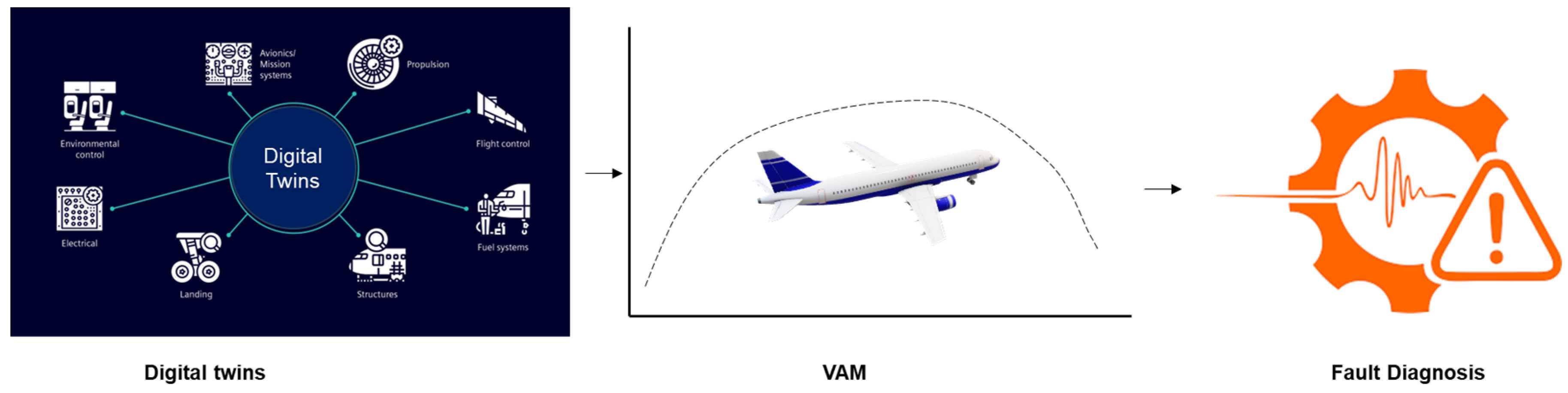
Figure 2.
Schematic for FAVER.
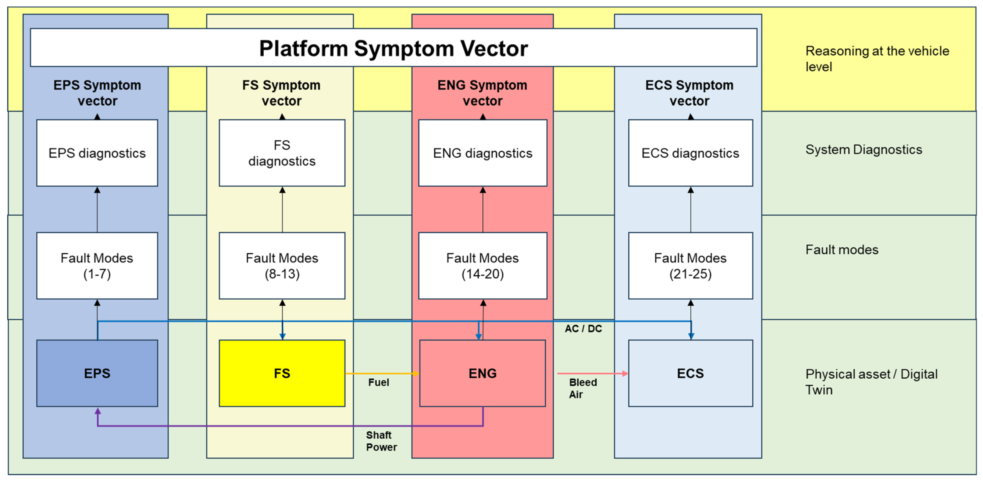
Figure 3.
Fuel rig located in the IVHM Centre Laboratory at Cranfield University.
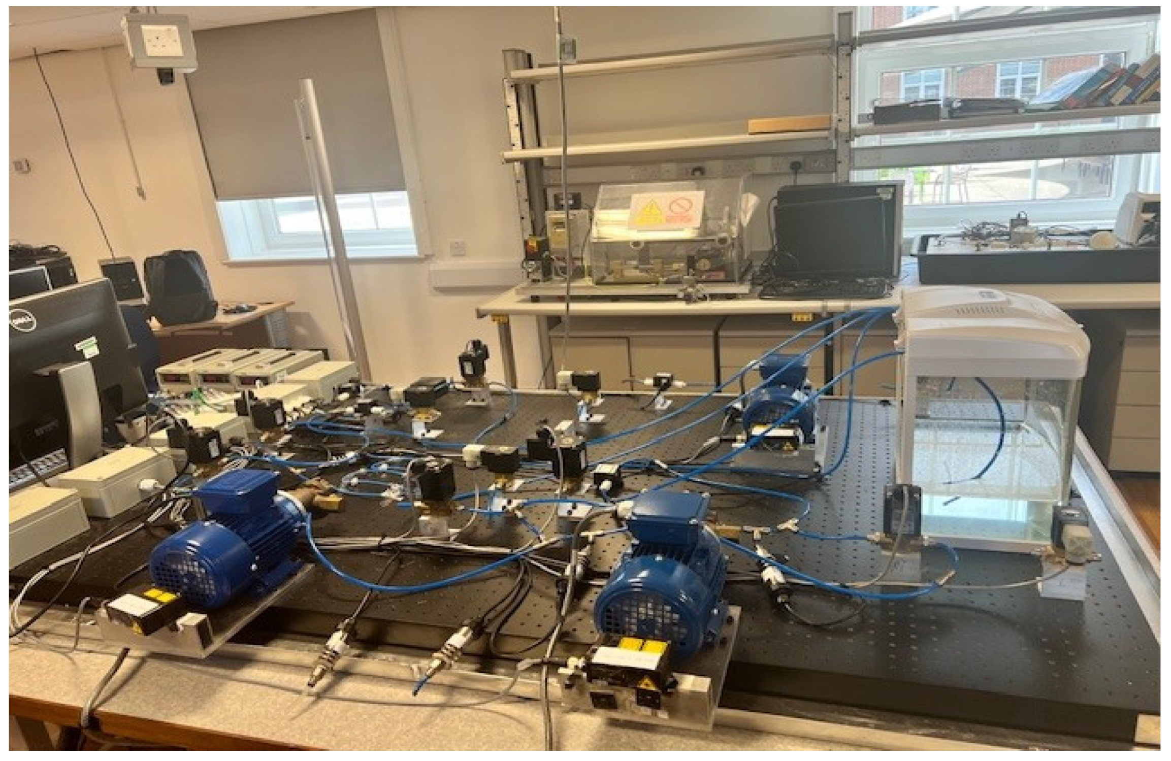
Figure 4.
Virtual aircraft model (VAM).
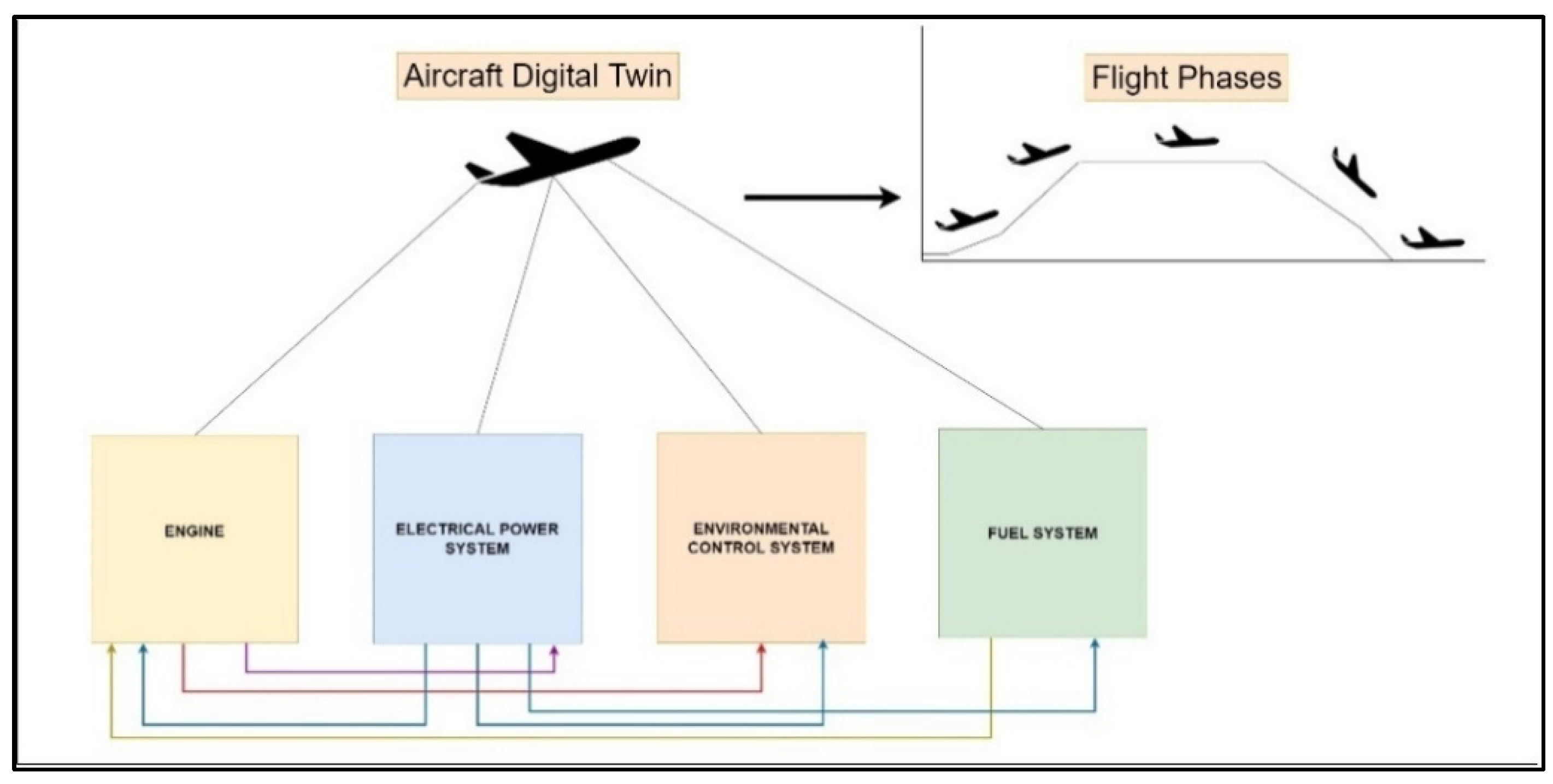
Figure 5.
Chosen flight profile.
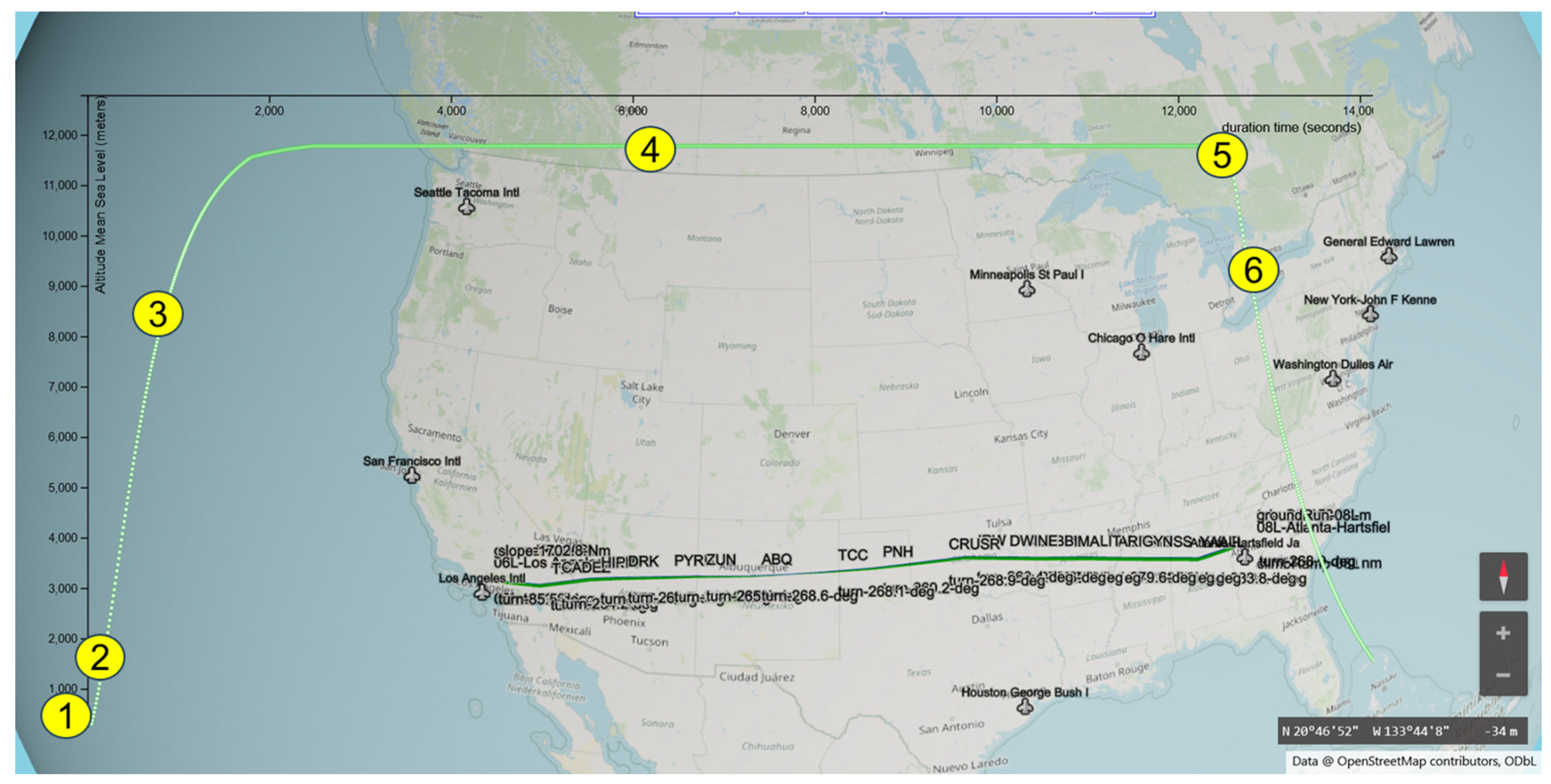
Figure 6.
Extension to FAVER.
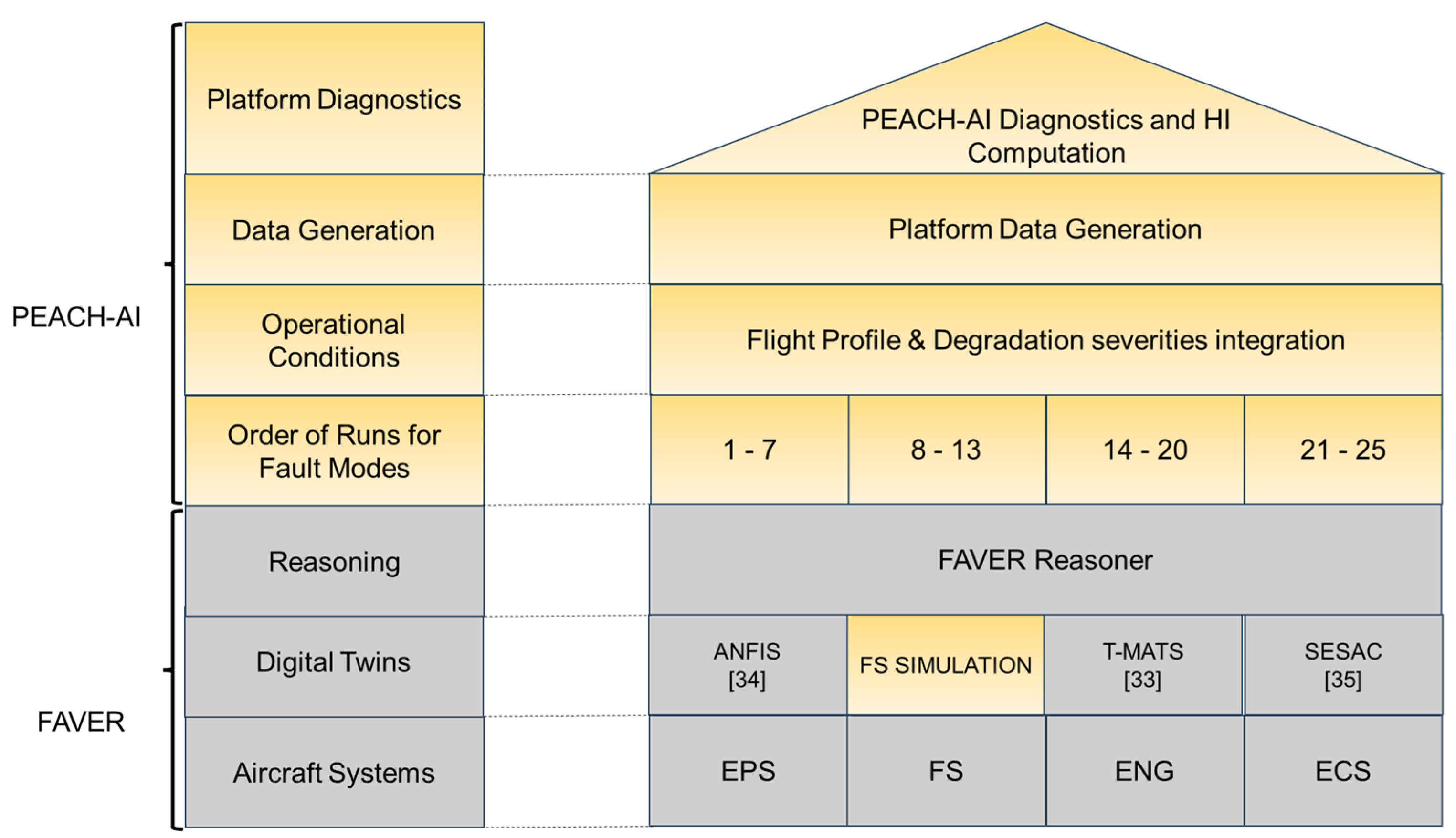
Figure 7.
Order of runs.
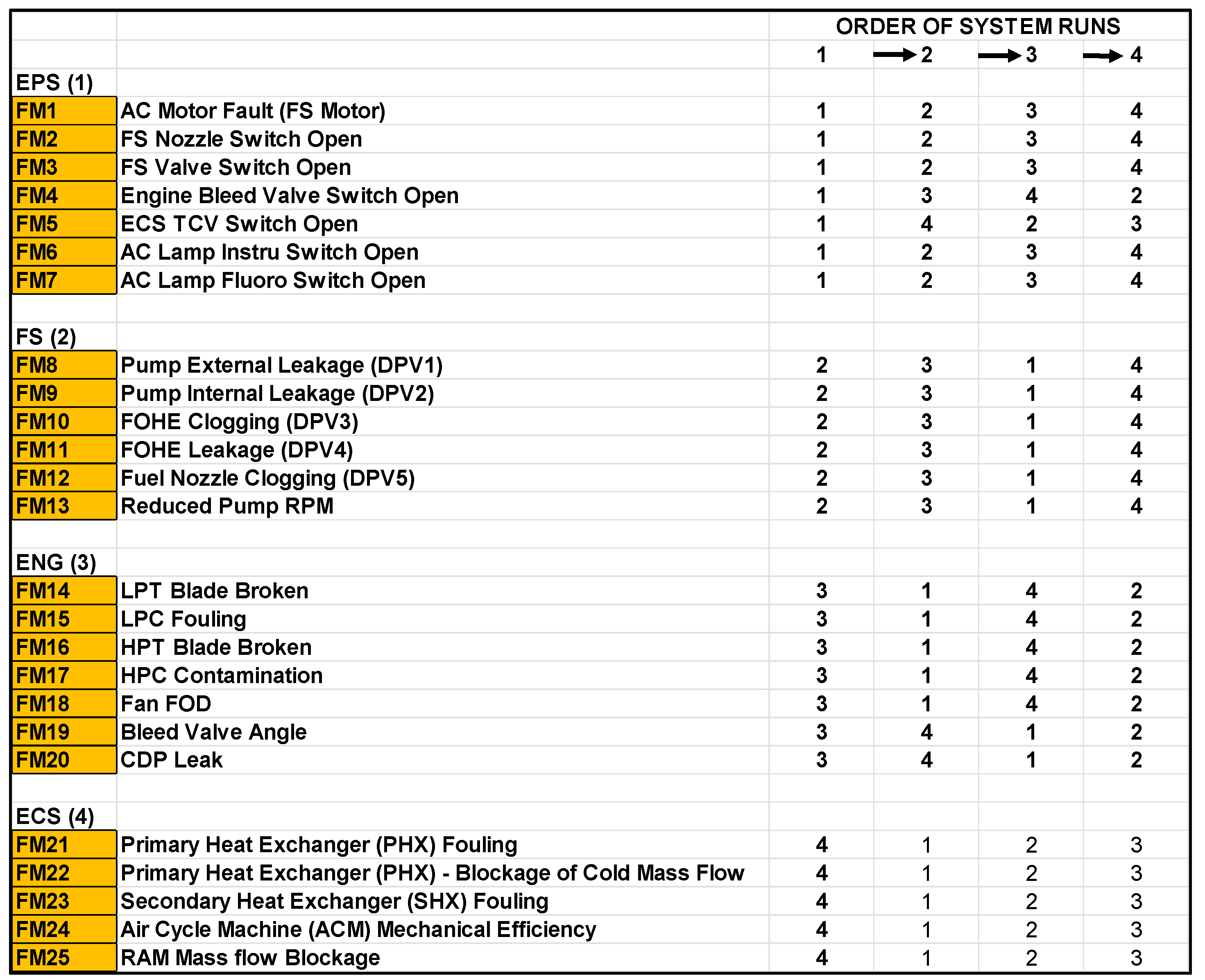
Figure 10.
System run on the VAM.
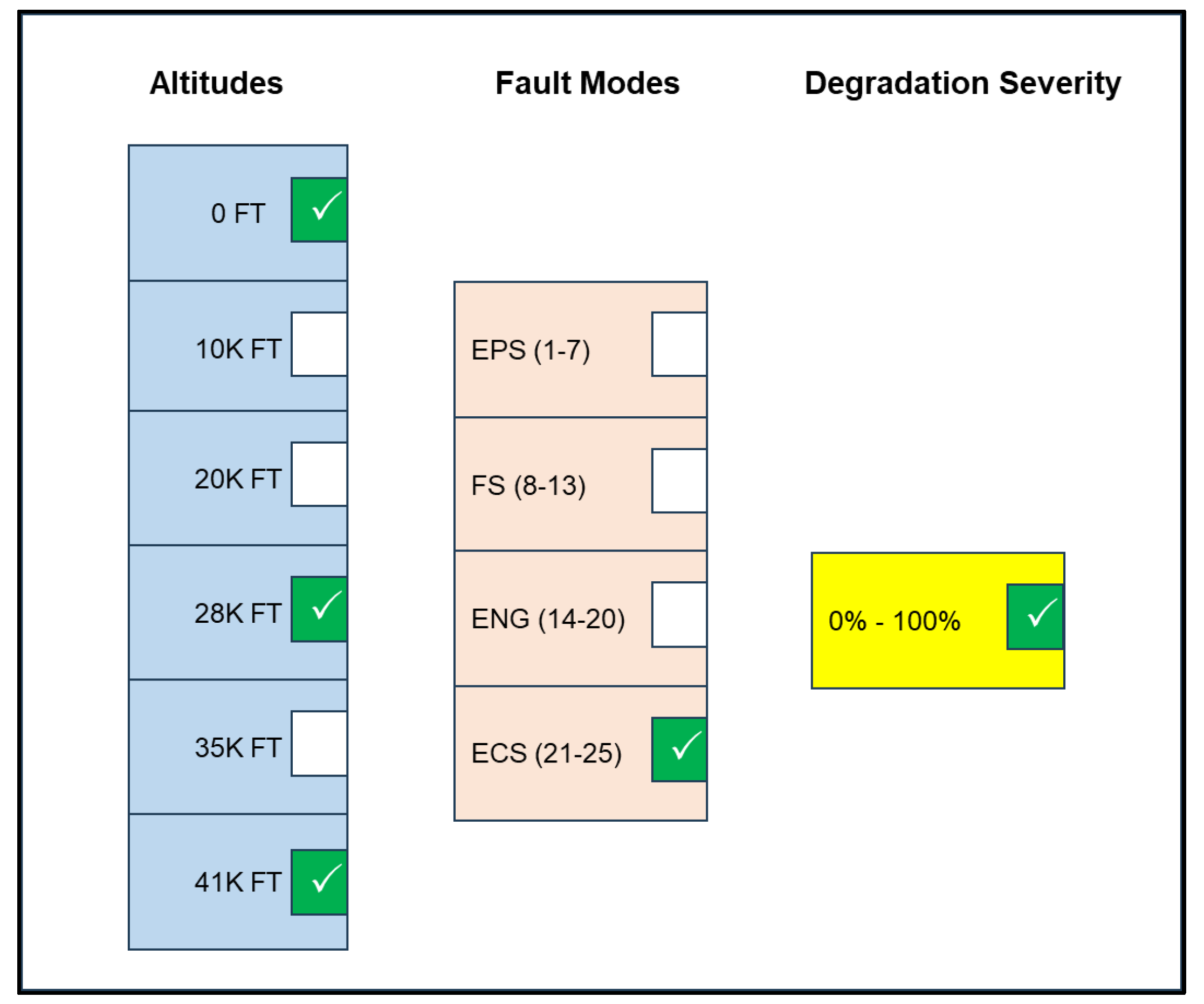
Figure 11.
Platform run on the VAM.
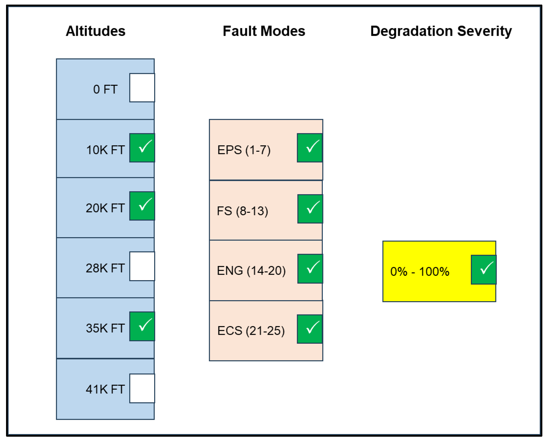
Figure 12.
Initial SoH results.
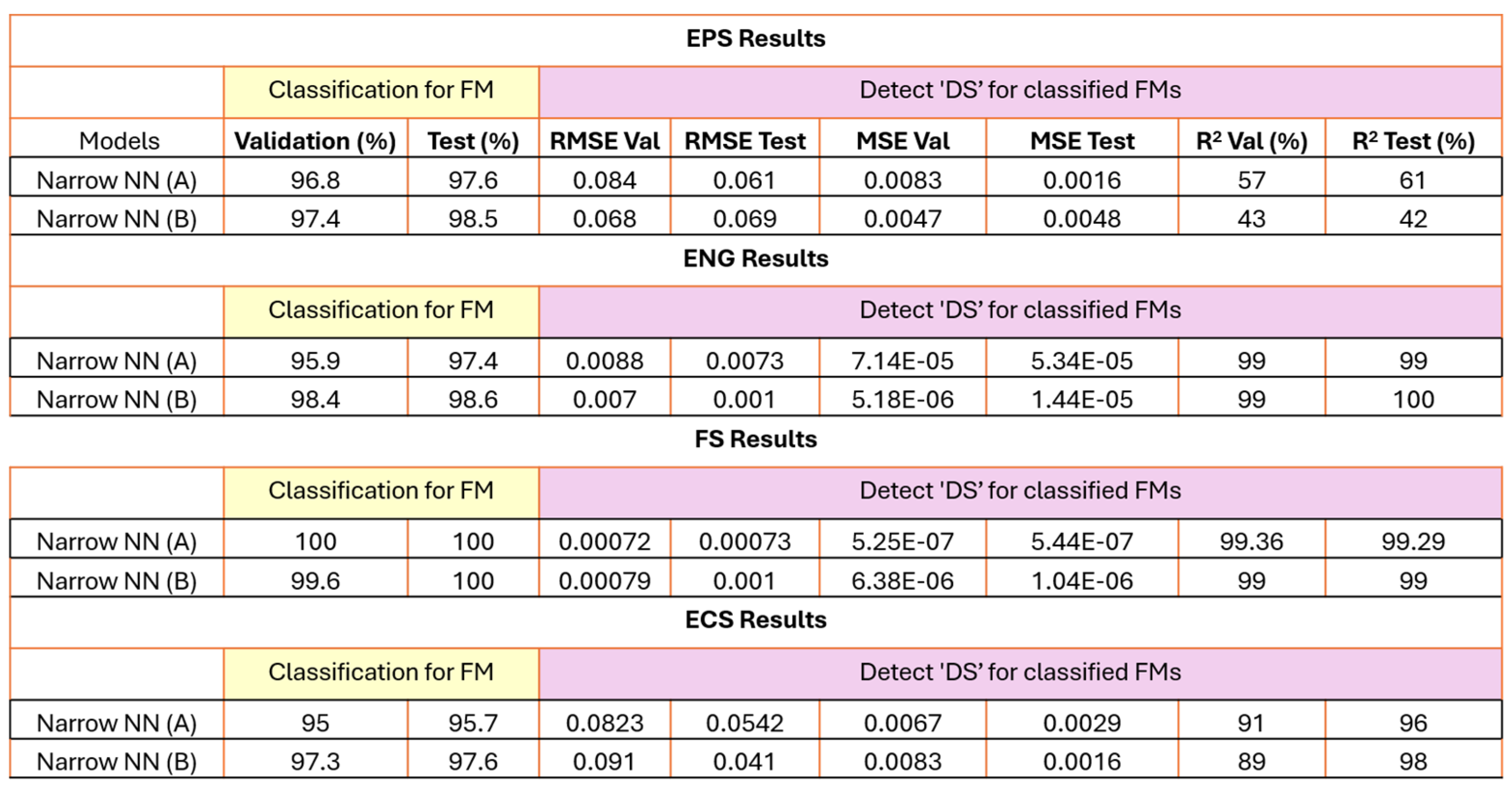
Table 1.
Systems and fault modes in FAVER.
| System | Fault Mode |
| Electrical Power System (EPS) | FS AC Motor Fault (FM1) |
| FS Nozzle Switch Fault (FM2) | |
| FS Valve Switch Fault (FM3) | |
| Engine Bleed Valve Switch Fault (FM4) | |
| ECS TCV Switch Fault (FM5) | |
| AC Lamp Instru Switch Fault (FM6) | |
| AC Lamp Fluoro Switch Fault (FM7) | |
| Fuel System (FS) | Pump External Leakage (FM8) |
| Pump Internal Leakage (FM9) | |
| Fuel Oil Heat Exchanger Clogging (FM10) | |
| Fuel Oil Heat Exchanger Leakage (FM11) | |
| Fuel Nozzle Clogging (FM12) | |
| Reduced Pump Speed (FM13) | |
| Engine (ENG) | LPT Blade Damage (FM14) |
| LPC Contamination (FM15) | |
| HPT Blade Damage (FM16) | |
| HPC Fouling (FM17) | |
| Fan Foreign Object Damage (FOD) (FM18) | |
| Bleed Valve Stuck (FM19) | |
| CDP Leakage (FM20) | |
| Environmental Control System (ECS) | Primary Heat Exchanger Fouling (FM21) |
| Primary Heat Exchanger - Blockage of Cold Mass Flow (FM22) | |
| Secondary Heat Exchanger Fouling (FM23) | |
| Air Cycle Machine Mechanical Efficiency Reduction (FM24) | |
| Ram Mass Flow Blockage (FM25) | |
Table 2.
System Symptom Vectors (SSVs) and Platform Symptom Vectors (PSV).
| Features | Description | EPS (SSV) | FS (SSV) | ENG (SSV) | ECS (SSV) | PSV |
| Altitude | Aircraft Altitude | ✓ | ✓ | ✓ | ✓ | ✓ |
| Mach_No | Mach Number | ✓ | ✓ | ✓ | ✓ | ✓ |
| Thrust_dmd | Thrust Demand | ✓ | ✓ | ✓ | ✓ | ✓ |
| DS | Degradation Severity | ✓ | ✓ | ✓ | ✓ | ✓ |
| FaultMode | Fault Mode | ✓ | ✓ | ✓ | ✓ | ✓ |
| P2 | Fuel System Pressure at Point 2 | ✓ | ✓ | |||
| P3 | Fuel System Pressure at Point 3 | ✓ | ✓ | |||
| P4 | Fuel System Pressure at Point 4 | ✓ | ✓ | |||
| P5 | Fuel System Pressure at Point 5 | ✓ | ✓ | |||
| P7 | Fuel System Pressure at Point 7 | ✓ | ✓ | |||
| Flow | Fuel Flow Rate | ✓ | ✓ | |||
| Tt_S5 | Total Temperature at Station 5 | ✓ | ✓ | |||
| Pt_S24 | Total Pressure at Station 24 | ✓ | ✓ | |||
| CoreSpeed | Engine Core Speed | ✓ | ✓ | |||
| Wf | Fuel Flow to Engine | ✓ | ✓ | |||
| Pt_AfCDP | Total Pressure after Custom Discharge Pressure | ✓ | ✓ | |||
| Tsfc | Thrust Specific Fuel Consumption | ✓ | ✓ | |||
| Power_GenOnly | Power Output from Generator | ✓ | ✓ | |||
| Power_AC_Gen_load | Power Load from AC Generator | ✓ | ✓ | |||
| Power_FSPump | Power Consumption by Fuel System Pump | ✓ | ✓ | |||
| Power_ACLamp | Power Consumption by AC Lamp | ✓ | ✓ | |||
| Power_TRU | Power distributed to the Transformer Rectifier Unit | ✓ | ✓ | |||
| FS_Motor_Torque | Fuel System Motor Torque | ✓ | ✓ | |||
| AC_Fluoro_I | Current in cabin window fluorescent lights | ✓ | ✓ | |||
| AC_Fluoro_V | Voltage in cabin window fluorescent lights | ✓ | ✓ | |||
| AC_Instru_V | Cockpit instrument panel lights | ✓ | ✓ | |||
| Eng_BleedValve_I | Current in Engine Bleed Valve | ✓ | ✓ | |||
| Eng_BleedValve_V | Voltage in Engine Bleed Valve | ✓ | ✓ | |||
| PVOT | Primary Valve Outlet Temperature | ✓ | ✓ | |||
| ThiPHX | Primary Heat Exchanger Inlet Temperature | ✓ | ✓ | |||
| ThoPHX | Primary Heat Exchanger Outlet Temperature | ✓ | ✓ | |||
| TiC | Compressor Inlet Temperature | ✓ | ✓ | |||
| ToC | Compressor Outlet Temperature | ✓ | ✓ | |||
| ThiSHX | Secondary Heat Exchanger Inlet Temperature | ✓ | ✓ | |||
| ThoSHX | Secondary Heat Exchanger Outlet Temperature | ✓ | ✓ | |||
| ThiRHX | Reheater Inlet Temperature | ✓ | ✓ | |||
| ThoRHX | Reheater Outlet Temperature | ✓ | ✓ | |||
| ThiCHX | Condenser Hot Inlet Temperature | ✓ | ✓ | |||
| ThoCHX | Condenser Heat Exchanger Outlet Temperature | ✓ | ✓ | |||
| TciRHX | Reheat Heat Exchanger Cold Inlet Temperature | ✓ | ✓ | |||
| TcoRHX | Reheat Heat Exchanger Cold Outlet Temperature | ✓ | ✓ | |||
| TiT | Turbine Inlet Temperature | ✓ | ✓ | |||
| ToT | Turbine Outlet Temperature | ✓ | ✓ | |||
| TcoCHX | Condenser Cold Outlet Temperature | ✓ |
Table 3.
Solution vector parameters and their ranges.
| Parameter | Definition | Range | Description |
| i | Flight phase being analysed. | Taxi (0 ft), Take-off (10,000 ft), Climb (20,000 ft), Cruise (28,000 ft), Top of Descent (35,000 ft), Descent (41,000 ft). | The altitude and phase of flight being simulated. |
| j | Fault type or fault mode. | 25 fault modes (7 for EPS, 6 for FS, 7 for ENG, 5 for ECS). | The specific fault modes within each system. |
| k | Degradation severity of the fault. | 0% (healthy) to 60% degradation | The severity of the fault. |
| l | Order of run for the fault mode. | Number of systems in the VAM | The sequence in which fault modes are simulated across systems. |
Disclaimer/Publisher’s Note: The statements, opinions and data contained in all publications are solely those of the individual author(s) and contributor(s) and not of MDPI and/or the editor(s). MDPI and/or the editor(s) disclaim responsibility for any injury to people or property resulting from any ideas, methods, instructions or products referred to in the content. |
© 2025 by the authors. Licensee MDPI, Basel, Switzerland. This article is an open access article distributed under the terms and conditions of the Creative Commons Attribution (CC BY) license (http://creativecommons.org/licenses/by/4.0/).
Copyright: This open access article is published under a Creative Commons CC BY 4.0 license, which permit the free download, distribution, and reuse, provided that the author and preprint are cited in any reuse.


