
Submitted:
26 March 2025
Posted:
26 March 2025
You are already at the latest version
Abstract
This study examines the drivers of inflation in Angola over the period 2015–2024 (120 observations), using an autoregressive distributed lag (ARDL) model. By integrating key macroeconomic variables such as the consumer price index (CPI), trade-weighted inflation (TCPI), nominal exchange rate (EXR), and money supply (M2), the research investigates both short-run dynamics and long-run equilibrium relationships. The analysis applies unit root tests and ARDL bounds testing to confirm cointegration among the variables and employs Granger causality tests to explore directional influences. Results indicate that inflation in Angola exhibits strong persistence with significant adjustment toward long-run equilibrium, while external shocks, particularly exchange rate fluctuations, play a critical role in influencing price levels. Monetary policy transmission and fiscal discipline appear to have limited immediate impact, suggesting that structural factors and reliance on oil revenues are major contributors to inflationary pressures. Based on these findings, the study recommends improvements in foreign exchange management, enhancement of domestic production capacity, diversification of the economy, and tighter fiscal controls.
Keywords:
inflation
; ARDL model
; monetary policy
; Angola
1. Introduction
Since gaining independence in 1975, Angola’s economy has experienced significant transformations, marked by socialist policies, civil war (1975–2002), and economic instability. According to Figure 1 below, post-war, from 2002 to 2014, Angola saw rapid oil-driven growth averaging 10 percent, enabling infrastructure development but deepening dependence on oil. The 2014 oil price collapse led to recession (2016–2020), currency depreciation, and inflation. Since 2018, reforms focusing on exchange rate liberalization, fiscal consolidation, and diversification have stabilized the economy, though structural challenges persist. The economy rebounded modestly in a post-recession, growing 4.4 percent in 2024, a fourth-year consecutive growth, averaging 2.4 percent, but oil remains central to Angola’s economy, accounting for about 29 percent of GDP, 59 percent of government revenues, and 94 percent of exports (INE, Ministry of Finance of Angola and BNA). Nevertheless, diversification efforts are yielding results, as agriculture is regaining its position as the primary driver of non-oil GDP, fueled by increased credit to the agricultural sector [1,2].
Inflation in Angola has historically been volatile due to war, economic transitions, and external shocks. The country faced hyperinflation in the 1990s, exceeding 4,000 percent, driven by excessive money printing and fiscal mismanagement. Post-war reforms and oil revenue stabilization helped reduce inflation, which fell from 430 percent in 2000 to around 12 percent in 2006. Monetary policy has played a crucial role in inflation control. The “hard kwanza” policy introduced in 2003, involving exchange rate stabilization and foreign financing of deficits, helped control inflation. From 2003, tighter monetary policy reduced inflation, but persistent money growth, remonetization, and reserve accumulation kept inflation dynamics unstable.
The 2014 oil crisis and exchange rate depreciation led to inflation exceeding 36 percent in 2016–2017. Figure 2 shows Angola’s monthly inflation (month-on-month, MoM) trajectory from January 2015 to October 2024. Inflation peaked at 4.26 percent in July 2016, likely due to currency depreciation and economic instability. From 2017 to 2021, inflation remained volatile but relatively stable. A sharp decline occurred in early 2022, reaching 0.07 percent, possibly due to policy interventions. Inflation rebounded in 2023, peaking before settling at 1.70 percent in late 2024. The trend reflects inflationary pressures, economic adjustments, and policy impacts over time.
The relationship between money growth and inflation has been complex. Before 2015, Angola relied on foreign reserves to stabilize prices through exchange rate management. However, declining oil revenues forced a shift toward tighter monetary policies. Money supply fluctuations were notable, with growth peaking at 29 percent in 2021. Periods of excessive money growth, particularly in 2019 and 2020, may have contributed to inflation acceleration.
Angola’s fiscal policy has improved since 2000, with government expenditures declining from 60 percent of GDP in 2000 to 35 percent in 2008. However, spending increased post-2007, leading to a rising non-oil primary deficit. Inflation remains sensitive to global commodity prices, exchange rate movements, and fiscal discipline.
Looking at the variables considered for this study, Figure 3 shows weak correlations between CPI and M2 (–0.0237) and EXR (–0.1052), while TCPI has a significant negative correlation (–0.3052, p = 0.0007). Figure 4 confirms no strong relationship between inflation and M2. Figure 5 shows a weak link between CPI and EXR. Figure 6 highlights a negative trend between inflation and TCPI. These weak linear associations suggest further analysis using an econometric model to capture lagged effects.
Hence, this study proposes to quantify the impact of the determinants of inflation in Angola and to propose what policy measures might help ensure stable prices in Angola.
1.1. Research Questions
This research seeks to answer the following research questions:
- (i)
- Which independent variables contribute the most to inflation in Angola?
- (ii)
- What policy recommendations are necessary to help mitigate the impact of independent variables on inflation in Angola?
1.2. Research Objectives
This research primarily aims to analyze and measure the relationship between inflation and identified determinants in Angola. Using an autoregressive distributed lag (ARDL) model and subsequent diagnostic tests, the study evaluates the significance of these factors in influencing inflation over both short- and long-term horizons, while also identifying the direction of causality. Understanding the bidirectional link between inflation and selected variables is essential for formulating effective monetary policy in Angola. Furthermore, this study seeks to explore similar findings and policy recommendations from international experiences through an in-depth literature review.
1.3. Hypothesis
The null and alternative hypotheses will be examined in line with this study’s objectives to assess whether the identified variables influenced inflation between 2015 and 2024:
- H0: Inflation in Angola is determined by the variables; and
- Ha: Inflation in Angola is not determined by the variables.
The hypotheses will be evaluated at a 5 percent significance level for both short- and long-term relationships. If the probability associated with the t-value is greater than the significance level, the null hypothesis will be retained. However, if the probability of the t-value is less than the significance level, the null hypothesis will be rejected.
1.4. Significance of the Research
The uniqueness of this study lies in the fact that no previous research has examined the determinants of inflation in Angola for the period 2015–2024, nor has imported inflation been considered as a contributing factor. The findings can aid Angolan policymakers in formulating more effective macroeconomic policies and implementing measures to stabilize prices, benefiting both the economy and society.
2. Literature Review
This section reviews theoretical and empirical literature on inflation determinants to better rationalize the monetary policy formulation. Various studies highlight domestic and external factors influencing inflation, leading to different but often similar conclusions. Key theories examined include monetary, structuralist, and quantitative theories of money. Understanding these determinants is essential for designing effective anti-inflationary policies to achieve price stability. The section also outlines the theoretical framework and hypotheses tested in this study.
2.1. Generic Studies on Inflation Determinants
Inflation has been widely studied in economic literature, with various theoretical frameworks explaining its determinants.
The classical view, based on Fisher’s Quantity Theory of Money, suggests that inflation is primarily a monetary phenomenon [3]. According to Friedman, “inflation is always and everywhere a monetary phenomenon,” implying that money supply growth exceeding economic growth leads to inflation [4]. Empirical studies such as McCandless and Weber confirm a strong long-run relationship between money supply and inflation [5].
Keynesian models argue that inflation results from excessive demand in the economy. The Phillips Curve suggests a trade-off between inflation and unemployment in the short run [6]. Blanchard and Fischer expanded on this by considering expectations and wage-setting behavior [7]. Gordon supports that cost-push inflation arises from supply-side shocks, such as rising input costs [8]. Factors such as oil price shocks as described by Hamilton [9] and exchange rate pass-through examined by Taylor [10] contribute to inflationary pressures. Structuralists such as Chenery and Syrquin emphasize supply-side constraints, such as weak infrastructure and market rigidities, in driving inflation, especially in developing economies [11]. The New Keynesian model by Clarida, Galí and Gertler [12] integrates expectations, rigidities, and policy credibility, highlighting the role of central banks in anchoring inflation expectations.
Inflation can be influenced by exchange rate fluctuations and external trade dynamics. Studies such as Dornbusch and Rogoff emphasize the impact of currency depreciation on inflation through import prices [13,14]. The Balassa-Samuelson effect suggests that inflation differentials between countries can be explained by productivity differences in tradable versus non-tradable sectors [15,16].
2.2. Empirical Studies on Inflation in Africa
In Sub-Saharan Africa, studies from Ajayi and Khan, and Kilindo confirm the role of monetary expansion as a key driver of inflation [17,18]. In West Africa, Ghana and Nigeria have experienced inflation due to excessive public spending and central bank financing of deficits as concludes Amoah & Mumuni, and Oyejide [19,20].
Fielding proves that many African economies are import-dependent, making exchange rate fluctuations a crucial determinant of inflation [21]. Furthermore, studies on Nigeria from Olomola and Adejumo and Ghana from Bawumia show strong exchange rate pass-through to domestic prices [22,23]. Collier and Gunning argue that terms-of-trade shocks, such as commodity price fluctuations, exacerbate inflation volatility in resource-rich economies [24].
Mkenda and Ndulu et al. highlight how poor infrastructure, supply chain inefficiencies, and weak market integration contribute to persistent inflation in Africa [25,26] and Timmer further argues that food price inflation is particularly relevant, as agriculture-dependent economies experience inflation due to supply shocks [27].
2.3. Case Studies on Inflation in Angola
Angola has experienced persistent inflation over the years, influenced by structural constraints, monetary policies, fiscal imbalances, and external shocks. Several studies have analyzed the determinants of inflation in Angola, focusing on different periods and policy regimes.
Ferreira studied Angola’s inflationary trends during the post-civil war period (2002–2006) and found that excessive money supply growth, coupled with weak monetary policy transmission, fueled inflation [28]. IMF identified high exchange rate pass-through as a major driver of inflation in Angola due to the country’s heavy reliance on imports, as depreciation of the Kwanza (AOA) significantly increases domestic prices [29]. Alves and Silva used a VAR model to assess the relationship between money supply (M2), exchange rate fluctuations, and inflation in Angola. Their findings confirm that monetary expansion and depreciation of Kwanza contribute to inflationary pressures [30].
Martins examined the impact of fiscal policies on inflation in Angola, highlighting the role of fiscal deficits and public sector wage increases in driving inflation [31], while Sobrinho and Mano argue that inflation in Angola is closely linked to government spending and public debt dynamics, as the government finances deficits through central bank borrowing, inflationary pressures increase [32]. World Bank found that Angola’s inflation spikes often coincide with fiscal expansion, especially during election cycles [33].
UNCTAD noted that Angola’s import dependency leads to structural inflation, as price fluctuations in global markets directly impact domestic prices [34], while Barros and Ramos highlighted how weak domestic production capacity in the agriculture and manufacturing sectors exacerbates inflation by limiting local supply and increasing reliance on costly imports [35]. Furthermore, Bastos and Domingos studied food price inflation in Angola, emphasizing the role of logistical challenges, poor infrastructure, and supply chain inefficiencies in keeping food prices high [36].
Ferreira and Neto linked Angola’s inflation volatility to oil price fluctuations, showing that revenue declines from falling oil prices often result in currency depreciation and inflation spikes [37] and Banco Nacional de Angola emphasized that inflation in Angola tends to rise when oil prices fall due to the impact on foreign exchange reserves and currency stability [38].
3. Research Structure and Methodology
3.1. Data Sources, Estimation Period and Econometric Tool
The high frequency data used to estimate the time series in the present study were extracted from the Angola Statistical Office (INE) and the National Bank of Angola (BNA). For the inflation rates from the top 20 trading partners, data was extracted from the Federal Reserve Bank of St. Louis (FRED). The time series data are monthly, covering the period from 2015 to 2024, a total of 120 observations.
For the estimation exercise, the STATA 14.2 econometric tool was used.
3.2. Selection of Variables
The selection of variables was guided by a combination of theoretical insights, empirical evidence, data availability, and statistical methods, all aligned with the research question and literature review. Data for four variables were collected, as shown in Figure 7 below.
3.3. Research Methodology and Model Design
The objective of this research is to assess the underlying causes of inflation in Angola using the ARDL econometric model. To verify the existence of the relationship between the variables in the model, the following hypotheses were raised:
H0: Inflation in Angola is mainly determined by the variables; and
Ha: Inflation in Angola is not mainly determined by the variables.
The methodology used to quantify the effect of different independent variables on inflation using an ARDL model was as follows:
- (i)
- Conducting the Augmented Dickey Fuller (ADF) unit root test to check the stationarity of variables. For the test, the basic equation applied by Nkoro et al. involves estimating the following regression equation [39]:where represents the change in the dependent variable at time ; represents the constant term (intercept); represents the lagged level of the dependent variable; is the sum of the lagged differences in the dependent variable, capturing the short-term dynamics; and is the error term (white noise);
- (ii)
- Selecting the optimal lag length for the ARDL model using the Akaike Information Criterion (AIC) and specifying the long-term ARDL model equation:
- (iii)
- Estimating the short-term relationship and adding the error correction term, which is that of the long-term regression but lagged for a period:where represents the change in the dependent variable between two time periods. The difference operator () typically indicates a first difference; is the intercept term or constant; is the change in the independent variable and is the coefficient that measures the effect of this change on the dependent variable ; is the key term in ECM, represents the lagged error correction term and represents the speed of adjustment toward long-term equilibrium.
- (iv)
- Performing the bounds testing for cointegration and estimating the long-term relationship, as well as the short-term dynamics, using the error correction model (ECM);
- (v)
- Conducting a series of diagnostic tests to validate the model:
Jarque-Bera test (Normality of residuals)
where n is the sample size; S is the sample skewness; and K is the sample kurtosis.
Multicollinearity test
where is the R-squared value obtained by regressing the j-th predictor on all other predictors.
Breusch-Godfrey LM test (Serial correlation)
where, ût–i denotes the lagged residuals; αi represents the regression coefficients; p is the number of restrictions imposed by H0, and εt is the white noise error term in the auxiliary regression that satisfies all the classical assumptions.
Breusch-Pagan test (Heteroscedasticity)
where is the dependent variable; , ,…, are independent variables, β0, β1,…, βk are the coefficients to be estimated, and ϵi denotes the residuals (errors).
CUSUM test (Stability)
where represents the recursive residuals. The cumulative sum is plotted over time to monitor the stability of the parameters.
Granger causality test
where, is the dependent variable; is the independent variable whose past values are being tested for predictive power; is the intercept, denotes the coefficients for the lagged values of Y; denotes the coefficients for the lagged values of X; is the error term; and p and q are the maximum lags for Y and X, respectively.
4. Data, Estimation Results and Discussion
Figure 8 presents the descriptive statistics for the variables involved, each with 120 observations. CPI and TCPI show moderate variability, with TCPI having a higher mean and standard deviation, indicating greater dispersion. EXR exhibits the highest variability, with a wide range (26.67) and significant standard deviation (5.18), suggesting volatile fluctuations. M2 also shows considerable variability but less extreme than EXR. Median values are lower than means for all variables, indicating right-skewed distributions. Overall, EXR appears the most volatile, while CPI is the most stable.
4.1. Optimal Lag Selection
Based on the information criterion results, the AIC was determined to be the most suitable, as it had the lowest value. The findings indicate that the optimal lag selection for each variable in the ARDL model is 1, 4, 2, and 0 for CPI, TCPI, EXR, and M2, respectively.
The equation would take the following shape:
4.2. Unit Root Tests
Figure 9 and Figure 10 present the ADF and PP unit root tests, assessing stationarity with and without trend. Results indicate mixed integration orders, with CPI, EXR, and M2 exhibiting I(0) and I(1) properties, while TCPI is strictly I(1). These findings justify ARDL modeling, accommodating both I(0) and I(1) variables.
4.3. ARDL Bound Tests Results for Cointegration
As seen above, the series were integrated in different orders, that is, with a combination of I(0) and I(1) series; hence, the ARDL bounds test was applied to the level of the variables to determine whether the variables had a long-term cointegration.
Figure 11 shows the ARDL bounds testing results. With an F-statistic of 4.608, the result exceeds the upper bound at the 5 percent significance level (4.35). This suggests strong evidence of cointegration, implying a long-run relationship among the variables at conventional significance levels, hence the null hypothesis of no cointegration is rejected. The ARDL model is retained.
4.4. ARDL Model Estimation Results
The variables CPI, TCPI, EXR, and M2 exhibit cointegration, indicating the presence of a long-term equilibrium relationship. Consequently, both the long-term and short-term models were estimated to analyze their dynamics.
4.4.1. Long-Term Relationship
With the existence of a long-term relationship between variables, the model could quantify the effect of independent variables on the dependent variables, measuring the effect of the explanatory variables on the explained variable, as shown in Figure 12 below.
The long-run estimation results indicate that CPI is highly persistent, with its lagged value (CPI L1) significantly influencing current inflation (p < 0.01). On the other hand, TCPI and EXR coefficients, including their lags, are statistically insignificant, suggesting no strong long-run impact on CPI. M2 also lacks statistical significance, implying a weak monetary influence. The model’s R-squared (0.7061) suggests a good fit, but some explanatory variables contribute minimally. The insignificant constant indicates no strong autonomous inflationary pressures independent of included factors.
4.4.2. Short-Term Relationship
Despite confirming a long-term relationship, the ARDL model highlights the importance of short-term dynamics for immediate insights, predictive power, policy guidance, model accuracy, and economic theory alignment in econometric and time series analysis.
According to short-run regression results in Figure 13, the ARDL (1, 4, 2, 0) model indicates that past inflation significantly influences current inflation (lagged CPI coefficient: 0.702, p = 0.004), suggesting strong inflation persistence. This suggests inflation perception may drive inflation, as businesses and consumers adjust prices and wages based on past trends, reinforcing inflationary pressures. The error correction term (ECT) is –0.976 (p = 0.000), implying that deviations from long-run equilibrium adjust rapidly, with approximately 98 percent correction per period. External price movements (dTCPI) and exchange rate changes (dEXR) are statistically insignificant, indicating a minimal short-run impact on domestic inflation. Money supply changes (dM2) also lack immediate effect. The model is statistically significant (p = 0.0158) but explains only 34 percent of inflation variability (Adj. R-squared = 0.3361), suggesting other unaccounted factors influence inflation dynamics.
4.5. Results of the Diagnostic Tests
Using the approach described in chapter 3, diagnostic tests were conducted to assess (i) normality, (ii) autocorrelation, (iii) heteroscedasticity, and (iv) model stability.
4.5.1. Normality Tests
Figure 14 presents the normality test for residuals. The Jarque-Bera statistic (48.038) and the high kurtosis (10.31) indicate significant deviation from normality. The skewness (1.03) suggests asymmetry, with a rightward tilt. The histogram confirms non-normal distribution, implying potential misspecification or the need for transformation in the model.
4.5.2. Multicollinearity Test
Figure 15 presents the variance inflation factor (VIF) results, assessing multicollinearity among explanatory variables. The VIF values for TCPI (1.75), EXR (1.75), and M2 (1.00) are all below the conventional threshold of 10, indicating no severe multicollinearity. The mean VIF (1.50) further confirms that independent variables are not highly correlated, ensuring reliable coefficient estimates in the ARDL model. No corrective measures, such as variable exclusion or transformation, are required.
4.5.3. Autocorrelation Test
Figure 16 presents the Breusch-Godfrey test for autocorrelation to check for serial correlation in the residuals. The chi-square statistic (0.962) with 1 degree of freedom yields a p-value of 0.3266, which is above the conventional 5 percent significance level. This means that the model does not suffer from autocorrelation issues, which is desirable for ensuring unbiased and efficient estimates.
4.5.4. Heteroscedasticity Test
Figure 17 below shows the heteroscedasticity test results. Since the p-value of 0.9995 is greater than the 0.05 significance level, the null hypothesis was not rejected. Hence, it confirms homoscedasticity.
4.5.5. Stability Tests
The CUSUM test (Figure 18) shows that the model’s residuals remain within the upper and lower bounds at a 5 percent significance level, suggesting no structural instability. However, the CUSUMSQ test (Figure 19) indicates possible instability, as the cumulative sum of squared residuals approaches the boundaries. This suggests potential variance instability in the model over time, warranting further examination. While the model appears largely stable, some variations in the long-run variance may require adjustments or robust checks to ensure reliable inference.
4.6. Causality Analysis Results
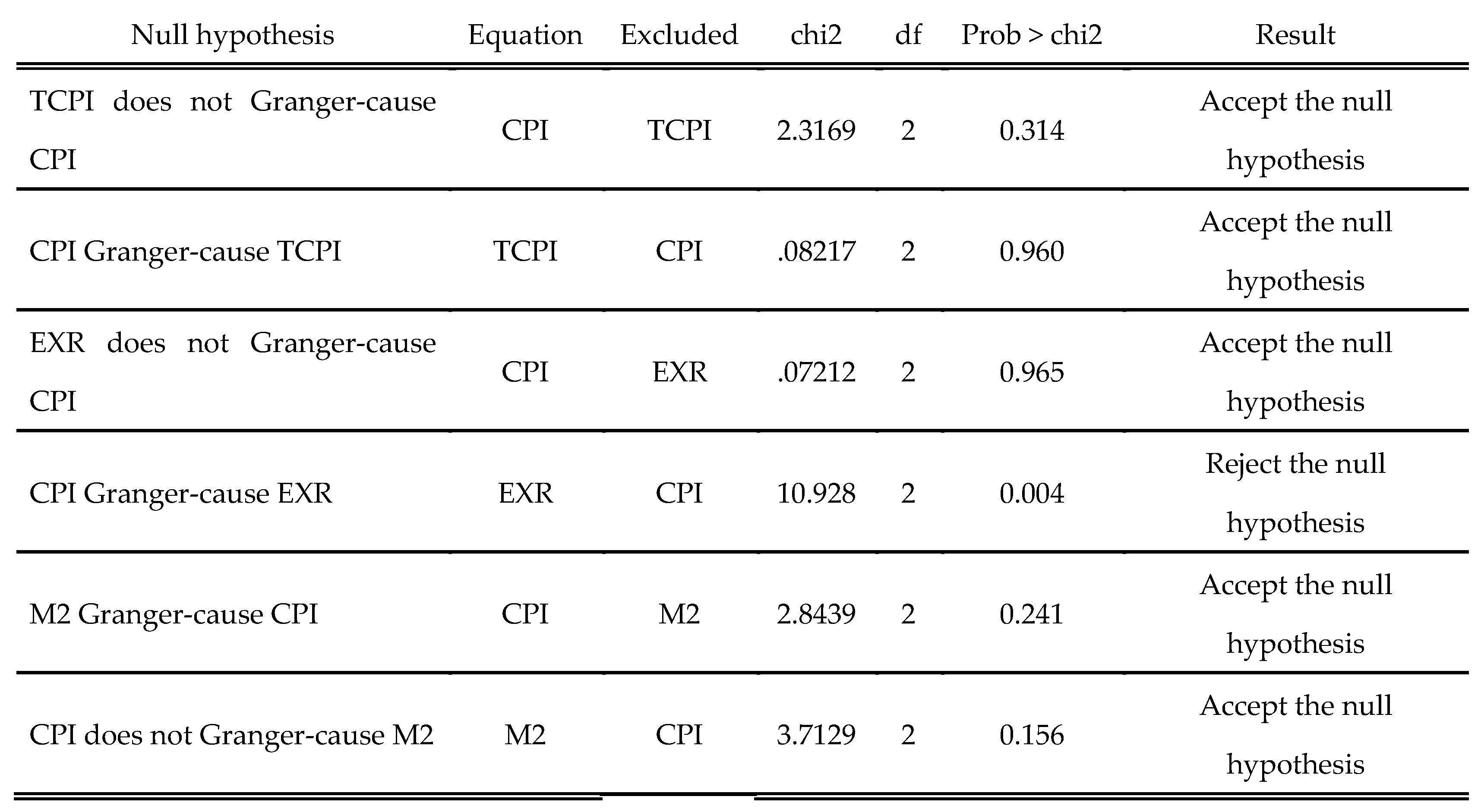
The Granger causality test results in Figure 20 below indicate that CPI Granger-causes EXR at a 1 percent significance level, while no bidirectional causality exists between CPI, TCPI, EXR, and M2. Other relationships fail to reject the null hypothesis.
4.7. Discussion
The ARDL model offers new insights into Angola’s inflation dynamics, reinforcing and extending prior research. Strong inflation persistence suggests inflation perception may be a key driver, as businesses and consumers adjust prices and wages based on past trends, supporting classical monetarist views. However, unlike traditional theories emphasizing money supply and fiscal deficits, the study findings indicate these factors (M2, TCPI) have limited short-run impact. Instead, exchange rate fluctuations play a crucial role, aligning with Ferreira (2006) and IMF reports, which highlight external shocks and currency depreciation as major determinants of domestic price movements.
Additionally, the weak statistical impact of fiscal measures echoes structuralist perspectives that stress the importance of underlying economic constraints, such as overdependence on oil revenues and insufficient domestic production. The discussion also emphasizes the role of monetary and fiscal policies in stabilizing inflation, suggesting that effective policy coordination is crucial for macroeconomic stability. Structural constraints, including weak domestic production capacity and limited financial inclusion, may exacerbate inflationary pressures. Furthermore, the findings are examined in the context of broader economic challenges, such as exchange rate pass-through effects and external debt sustainability. Thus, in contrast to the demand-pull and cost-push theories from Keynesian literature, the interplay between external variables and structural factors appears to dominate.
5. Conclusions
5.1. Summary Conclusions
The study on the drivers of inflation in Angola examines key macroeconomic variables influencing price levels. Using econometric techniques, it identifies exchange rate fluctuations, money supply growth, and external shocks as primary drivers of inflation. The findings highlight the significant role of exchange rate pass-through, given Angola’s reliance on imports and oil revenues. The study also reveals that monetary policy alone may be insufficient to control inflation without complementary fiscal measures. Structural weaknesses, such as limited domestic production and financial market inefficiencies, exacerbate inflationary pressures.
An optimal lag was selected, based on the AIC criterion, resulted in lags of 1 for CPI, 4 for TCPI, 2 for EXR, and 0 for M2, establishing the ARDL model structure. The ADF and PP unit root tests indicated mixed orders of integration among the variables, justifying the use of the ARDL methodology. Furthermore, the ARDL bounds test, where the F-statistic exceeds the critical value, confirmed cointegration and a stable long-term relationship. The long-term estimates reveal strong inflation persistence through significant lagged CPI effects, while short-term dynamics indicate that past inflation significantly influences current inflation, with a rapid error correction term adjusting nearly 98 percent of disequilibrium per period.
Subsequently, diagnostic tests affirmed normality, absence of multicollinearity, and no serial correlation, though the CUSUMSQ test hints at potential variance instability. Finally, in the Granger causality test it was revealed that CPI Granger-causes EXR, and the overall discussion in sub-chapter 4.7 emphasizes the need for coordinated policy actions to achieve price stability. Strengthening monetary policy transmission, improving foreign exchange management, and diversifying the economy are essential strategies to mitigate inflation risks. The study suggests enhancing domestic production capacity to reduce import dependency and implementing measures to stabilize the exchange rate. Fiscal discipline and improved public debt management are also critical for long-term stability. Overall, the research contributes to understanding inflation dynamics in resource-dependent economies, offering insights for policymakers.
On the other hand, the prevalence of a large informal economy in Angola (more than 80 percent of the population) could significantly impact the study’s findings. Since many transactions in the informal sector are not captured by official statistics, key variables such as money supply (M2) and the consumer price index (CPI) might be undermeasured. This under-reporting can lead to measurement error, thereby weakening the estimated relationships in the ARDL model. For example, if a substantial portion of economic activity occurs outside formal channels, the official monetary aggregates may not fully reflect the actual liquidity available, potentially biasing the estimated impact of money supply on inflation.
Moreover, the informal sector often operates with different pricing mechanisms and may experience more volatile price adjustments compared to the formal sector. As a result, the official CPI may not capture the full extent of price fluctuations, leading to a divergence between measured inflation and the inflation experienced by the public. This divergence could intensify inflation perception among consumers, which, in turn, may influence wage-setting behavior and demand for policy intervention. In summary, an extensive informal economy can compromise the robustness of the model’s variables and create a gap between official inflation measures and public inflation perceptions, thereby complicating policy design and effectiveness.
5.2. Policy Recommendations
To stabilize prices and support sustainable growth, Angola’s policymakers should strengthen monetary policy transmission to ensure effective interest rate adjustments, improve foreign exchange management to mitigate inflation from exchange rate fluctuations, and promote economic diversification and domestic production to reduce dependence on oil and imports. Furthermore, fiscal discipline should be enhanced through better debt management and deficit reduction, implement targeted interventions to stabilize food prices and support food security, and formalize the informal economy by improving data accuracy, incentivizing formalization, and tailoring policies to its unique dynamics, bridging gaps between official inflation measures and public perceptions for better policymaking.
5.3. Accomplishment of Research Objectives
The study used an ARDL model, diagnostic tests, and causality analysis to assess inflation determinants in Angola, international findings to refine policy recommendations for effective monetary management and long-term price stability.
5.4. Limitations of the Research
Due to limited high-frequency data, the study did not assess the impact of inflation perception, potential GDP, and the informal sector on inflation, which may influence overall price dynamics in Angola.
References
- Caetano Joao, M.A. Determinants of Sustainable Economic Growth in Angola: A Case Study on Agriculture. Sci Set J of Economics Res 2024, 3, 1–11. [Google Scholar]
- Caetano Joao, M.A.; Castro, A.M. The Impact of Agricultural Credit on the Growth of the Agricultural Sector in Angola. Sustainability 2023, 15, 14704. [Google Scholar] [CrossRef]
- Fisher, I. (1911). The purchasing power of money. Macmillan.
- Friedman, M. The role of monetary policy. American Economic Review 1968, 58, 1–17. [Google Scholar]
- McCandless, G.T.; Weber, W.E. Some monetary facts. Federal Reserve Bank of Minneapolis Quarterly Review 1995, 19, 2–11. [Google Scholar] [CrossRef]
- Phillips, A.W. The relation between unemployment and the rate of change of money wages in the United Kingdom, 1861–1957. Economica 1958, 25, 283–299. [Google Scholar] [CrossRef]
- Blanchard, O.J.; Fischer, S. (1989). Lectures on macroeconomics. MIT Press.
- Gordon, R.J. The role of wages in the inflation process. American Economic Review 1988, 78, 276–283. [Google Scholar]
- Hamilton, J.D. Oil and the macroeconomy since World War II. Journal of Political Economy 1983, 91, 228–248. [Google Scholar] [CrossRef]
- Taylor, J.B. Low inflation, pass-through, and the pricing power of firms. European Economic Review 2000, 44, 1389–1408. [Google Scholar] [CrossRef]
- Chenery, H.B.; Syrquin, M. (1975). Patterns of development, 1950–1970. Oxford University Press.
- Clarida, R.; Galí, J.; Gertler, M. The science of monetary policy: A New Keynesian perspective. Journal of Economic Literature 1999, 37, 1661–1707. [Google Scholar] [CrossRef]
- Dornbusch, R. Expectations and exchange rate dynamics. Journal of Political Economy 1976, 84, 1161–1176. [Google Scholar] [CrossRef]
- Rogoff, K. The purchasing power parity puzzle. Journal of Economic Literature 1996, 34, 647–668. [Google Scholar]
- Balassa, B. The purchasing-power parity doctrine: A reappraisal. Journal of Political Economy 1964, 72, 584–596. [Google Scholar] [CrossRef]
- Samuelson, P.A. Theoretical notes on trade problems. Review of Economics and Statistics 1964, 46, 145–154. [Google Scholar] [CrossRef]
- Ajayi, S.I.; Khan, M.S. (2000). External debt and domestic capital formation in sub-Saharan Africa. African Development Bank.
- Kilindo, A.A. (1997). Fiscal operations, money supply, and inflation in Tanzania. AERC Research Paper No. 65.
- Amoah, B.; Mumuni, Z. Fiscal expansion and inflation dynamics in West Africa. African Journal of Economic Policy 2019, 26, 45–61. [Google Scholar]
- Oyejide, T.A. Deficit financing, inflation, and capital formation: An analysis of the Nigerian experience, 1957–1970. Nigerian Journal of Economic and Social Studies 1972, 14, 27–43. [Google Scholar]
- Fielding, D. Inflation and political instability in Africa. Journal of Development Studies 2008, 44, 731–757. [Google Scholar]
- Olomola, P.A.; Adejumo, A.V. Oil price shock and macroeconomic activities in Nigeria. International Research Journal of Finance and Economics 2006, 3, 28–34. [Google Scholar]
- Bawumia, M. (2010). Exchange rate movements and inflation in Ghana: Evidence from a structural VAR. Bank of Ghana Working Paper.
- Collier, P.; Gunning, J.W. Explaining African economic performance. Journal of Economic Literature 1999, 37, 64–111. [Google Scholar] [CrossRef]
- Mkenda, B.K. Long-run and short-run determinants of real exchange rates in Africa. Journal of African Economies 2001, 10, 62–103. [Google Scholar]
- Ndulu, B.; O’Connell, S.A.; Bates, R.H.; Collier, P.; Soludo, C.C. (2007). The political economy of economic growth in Africa, 1960–2000. Cambridge University Press.
- Timmer, C.P. (2009). Rice price formation in the short run and the long run: The role of market structure in explaining volatility. Center for Global Development Working Paper No. 172.
- Ferreira, M. Inflation dynamics in Angola: The role of monetary policy and external factors. African Journal of Economic Studies 2006, 11, 89–106. [Google Scholar]
- International Monetary Fund (IMF). (2016). Angola: Selected issues (IMF Country Report No. 16/102). Washington, DC: IMF.
- Alves, J.; Silva, P. Money supply, exchange rates, and inflation in Angola: A VAR approach. Journal of African Economies 2018, 27, 350–372. [Google Scholar]
- Martins, J. The role of fiscal policy in inflation dynamics: Evidence from Angola. African Economic Policy Review 2015, 22, 112–129. [Google Scholar]
- Sobrinho, R.; Mano, D. Inflation and government spending: Angola’s fiscal dilemma. Economic Review of Southern Africa 2019, 15, 78–96. [Google Scholar]
- World Bank. (2021). Angola economic update: Strengthening the macro-fiscal framework to promote economic diversification. Washington, DC: World Bank.
- United Nations Conference on Trade and Development (UNCTAD). (2020). Trade and development report 2020. Geneva: UNCTAD.
- Barros, L.; Ramos, C. Inflation and food price volatility in Angola: A sectoral analysis. African Development Review 2017, 29, 512–529. [Google Scholar]
- Bastos, M.; Domingos, A. Logistical constraints and food price inflation in Angola. Economic Bulletin of Southern Africa 2019, 14, 65–82. [Google Scholar]
- Ferreira, M.; Neto, P. Oil price shocks and inflation volatility in Angola. Energy Economics 2013, 36, 446–457. [Google Scholar]
- Banco Nacional de Angola. (2022). Monetary policy report. Luanda, Angola: BNA.
- Nkoro, E.; Uko, A.K. Autoregressive distributed lag (ARDL) cointegration technique: Application and interpretation. Journal of Statistical and Econometric Methods 2016, 5, 63–91. [Google Scholar]
Figure 1.
GDP performance. Source: Author’s calculations in MS Excel using data series.
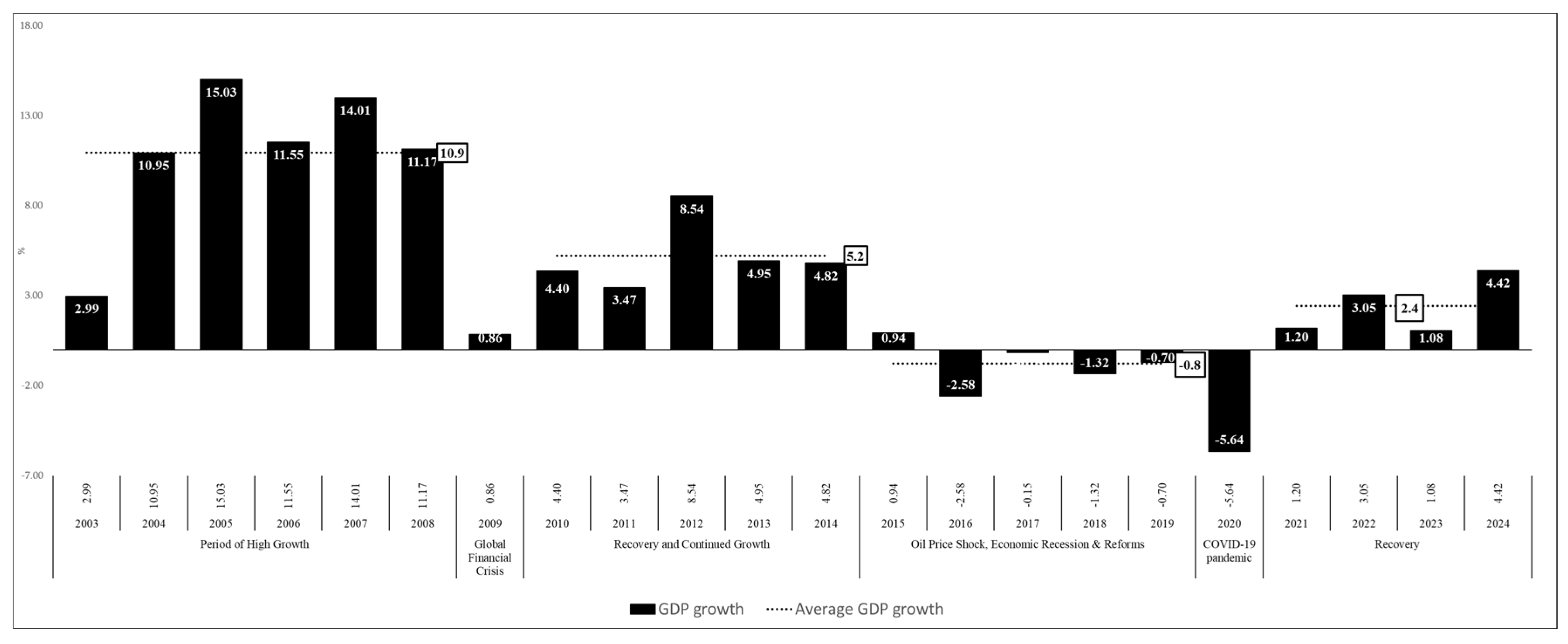
Figure 2.
Monthly inflation (MoM) trajectory in Angola. Source: Author’s calculations in MS Excel using data series.
Figure 2.
Monthly inflation (MoM) trajectory in Angola. Source: Author’s calculations in MS Excel using data series.
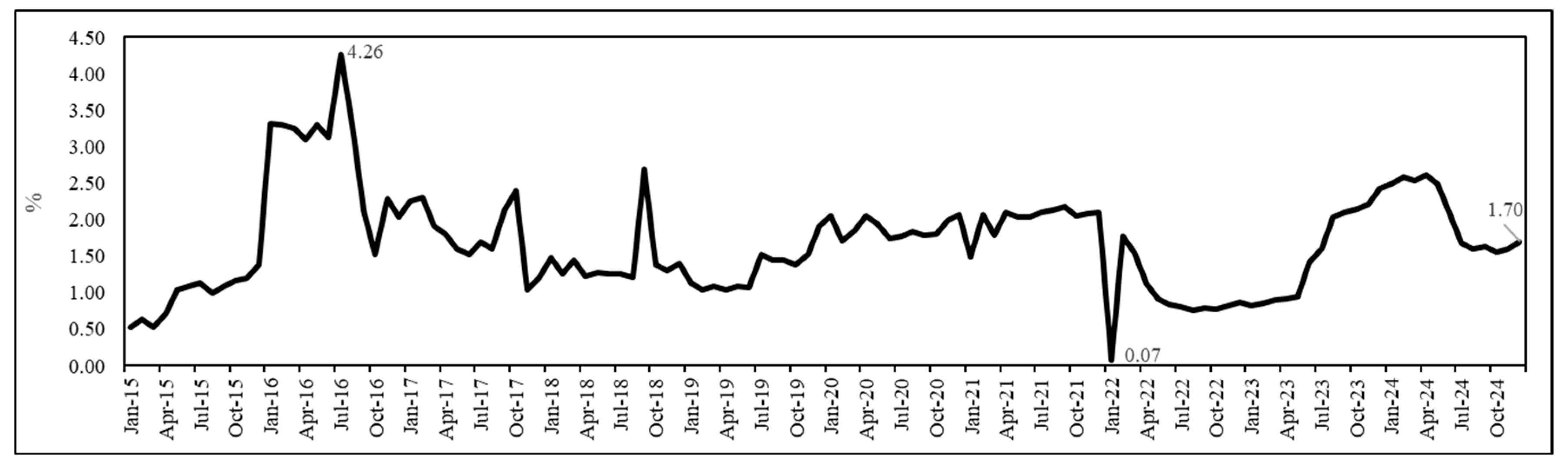
Figure 3.
Pearson correlation coefficients. Source: Author’s calculations in MS Excel using data series.
Figure 3.
Pearson correlation coefficients. Source: Author’s calculations in MS Excel using data series.
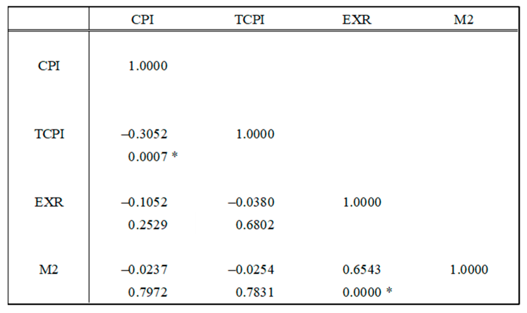
Figure 4.
Relationship between inflation and M2. Source: Author’s calculations in MS Excel using data series.
Figure 4.
Relationship between inflation and M2. Source: Author’s calculations in MS Excel using data series.
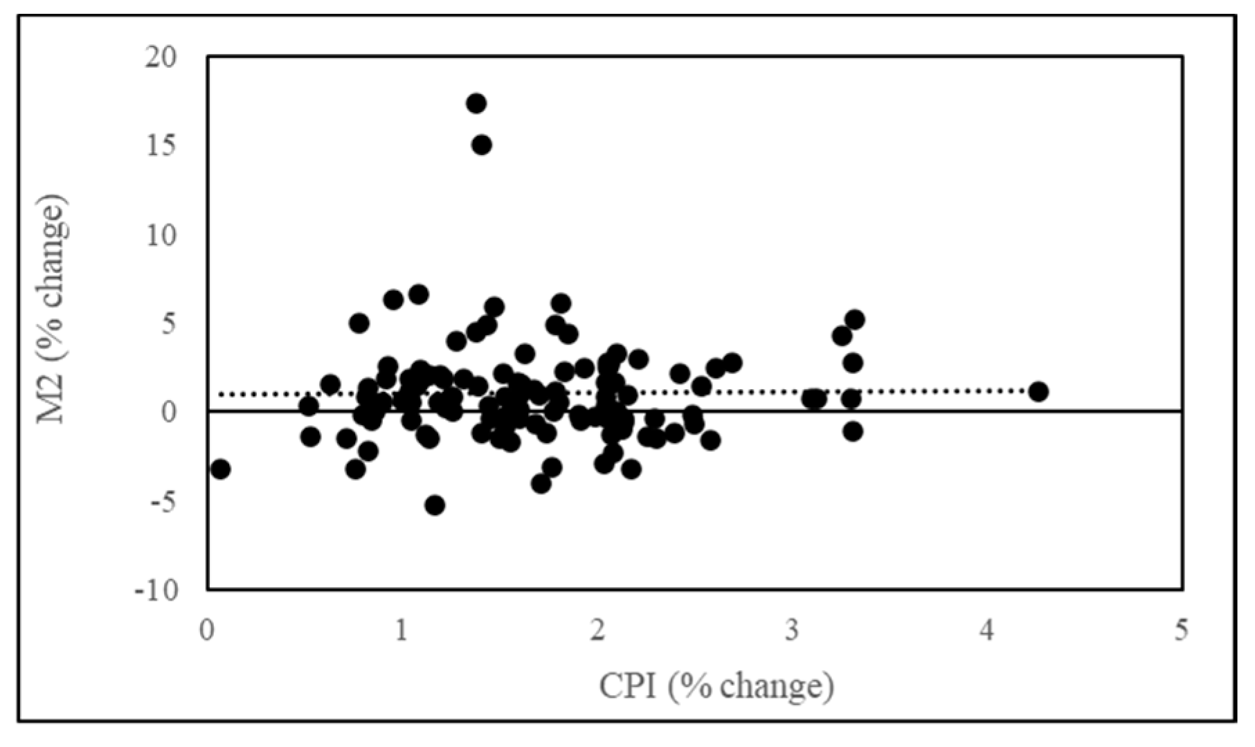
Figure 5.
Relationship between inflation and EXR. Source: Author’s calculations in MS Excel using data series.
Figure 5.
Relationship between inflation and EXR. Source: Author’s calculations in MS Excel using data series.
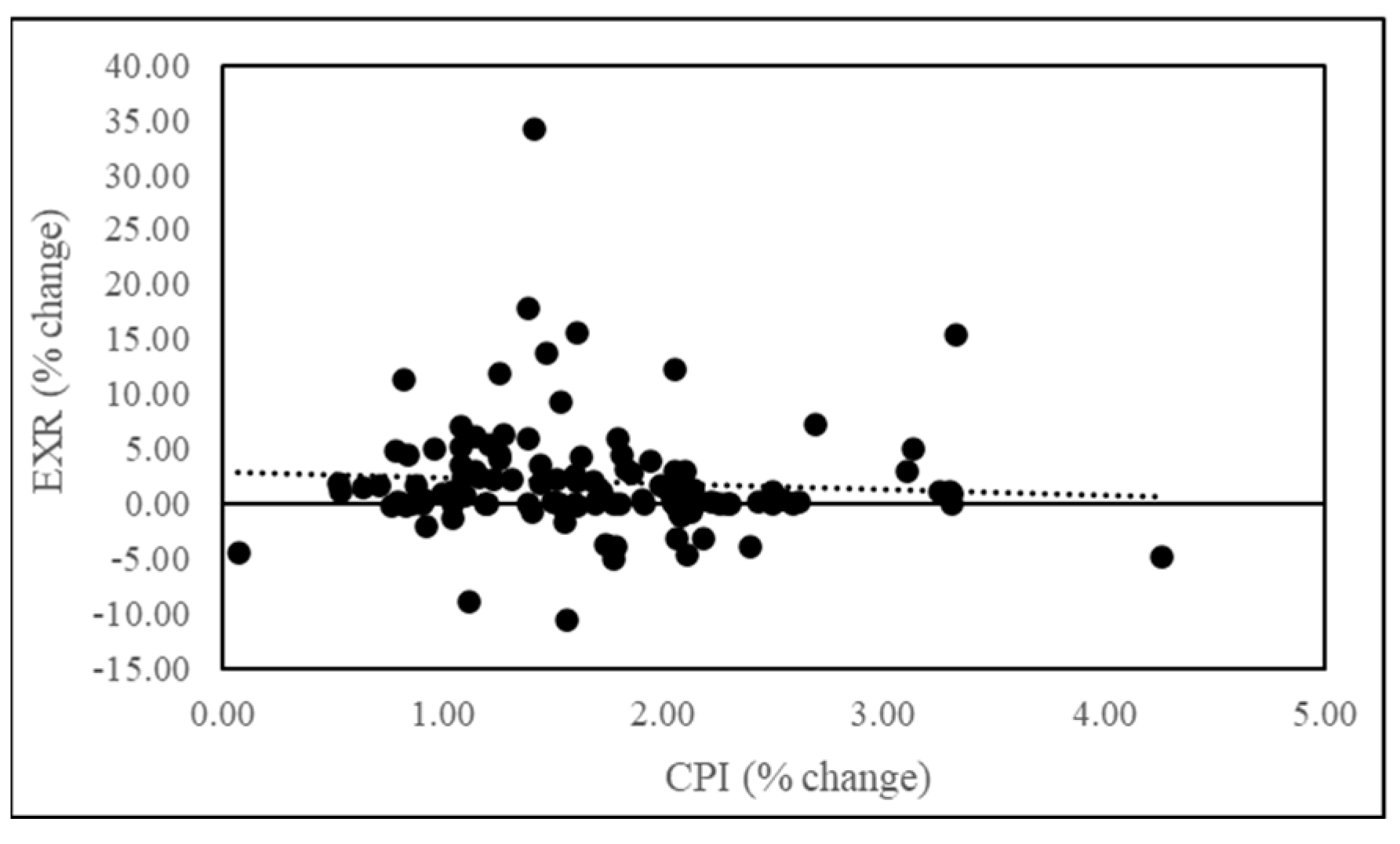
Figure 6.
Relationship between inflation and TCPI. Source: Author’s calculations in MS Excel using data series.
Figure 6.
Relationship between inflation and TCPI. Source: Author’s calculations in MS Excel using data series.
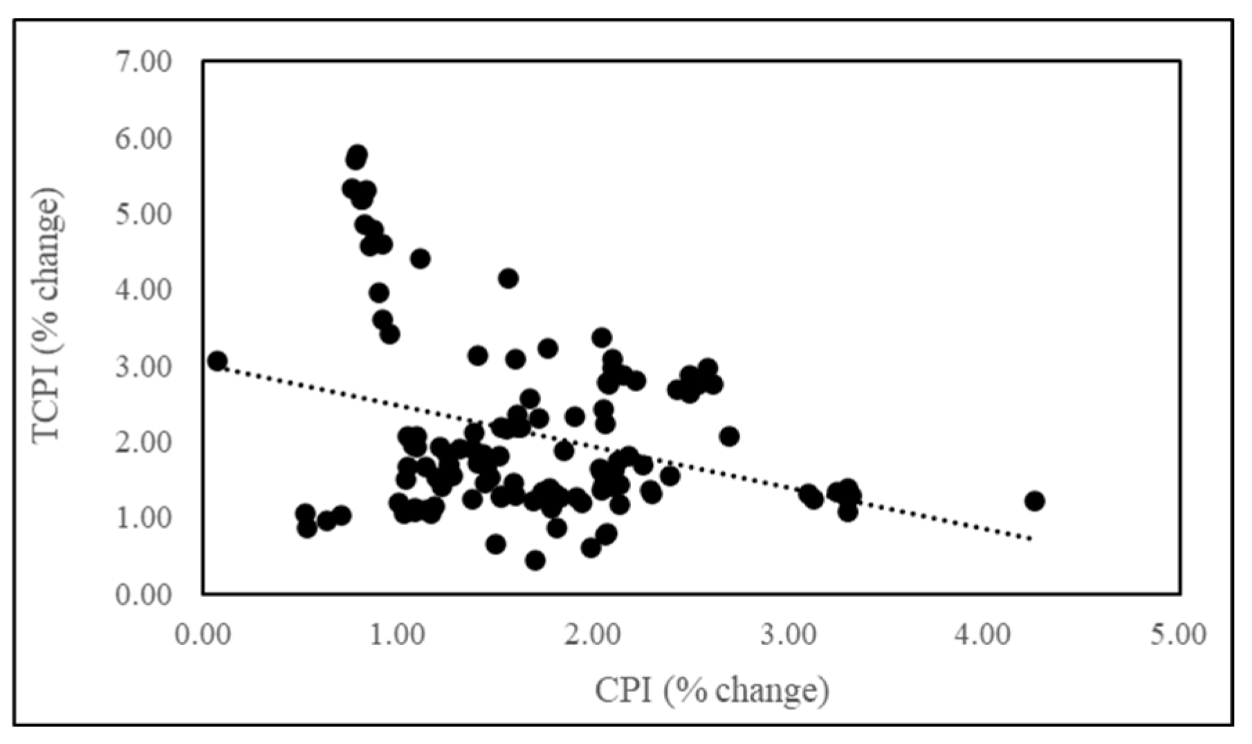
Figure 7.
Summary of dependent and independent variables used in the study.
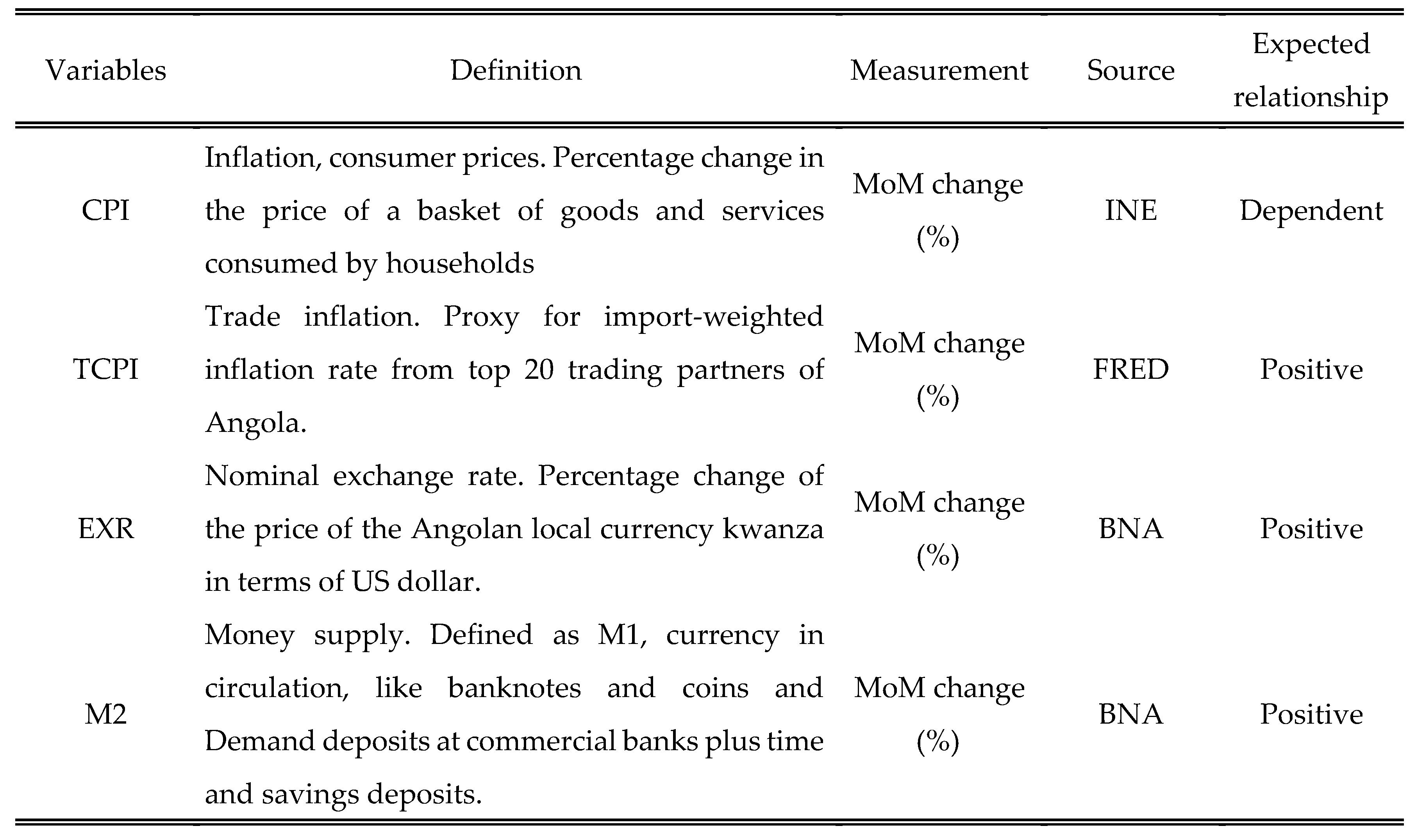
Figure 8.
Descriptive statistics results. Source: Authors’ computation using STATA 14.2.
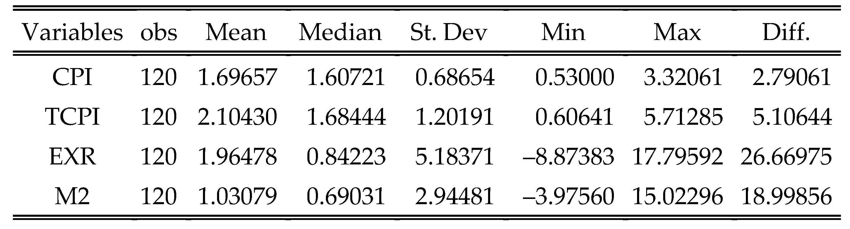
Figure 9.
ADF and PP unit root tests with intercept. Source: Author’s computation using STATA 14.2.
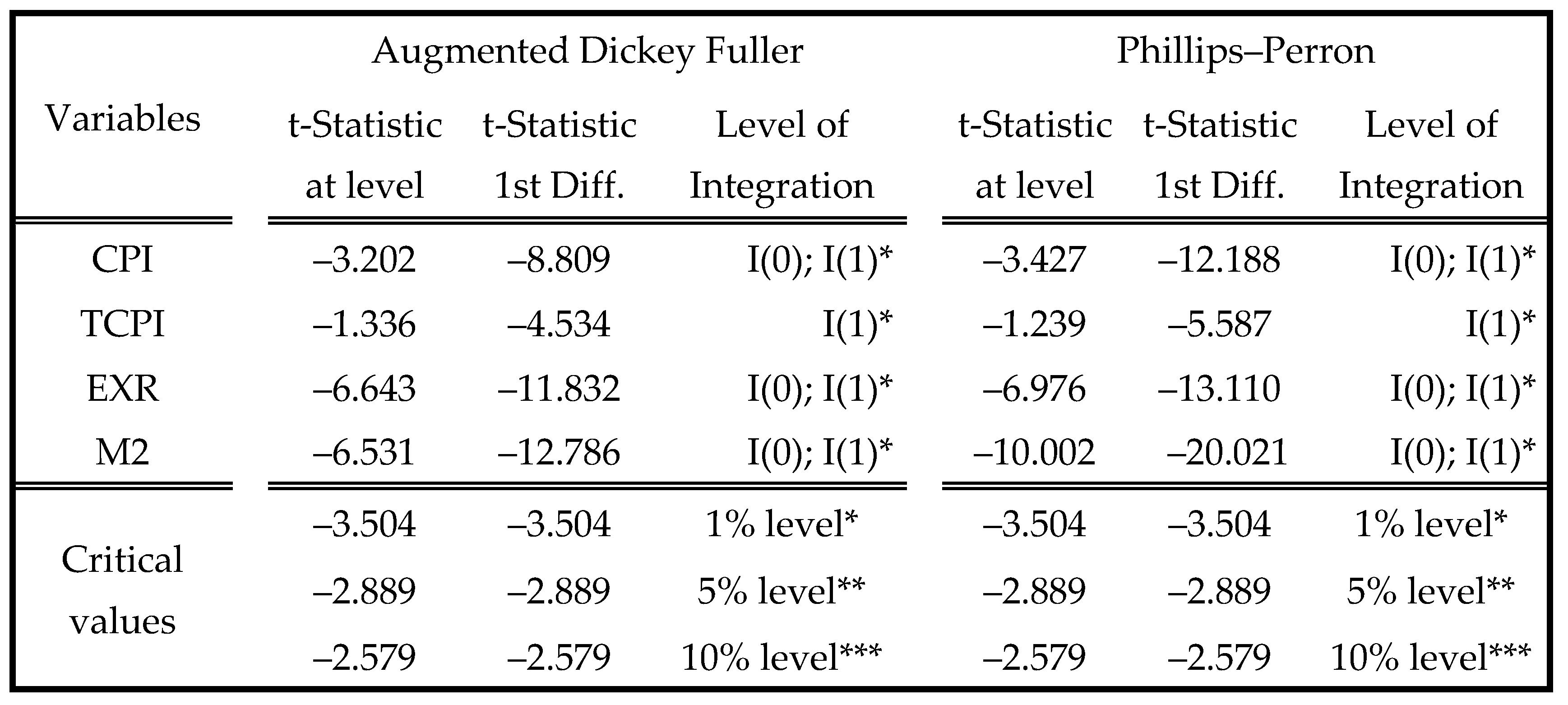
Figure 10.
ADF and PP unit root tests with intercept and trend. Source: Author’s computation using STATA 14.2.
Figure 10.
ADF and PP unit root tests with intercept and trend. Source: Author’s computation using STATA 14.2.
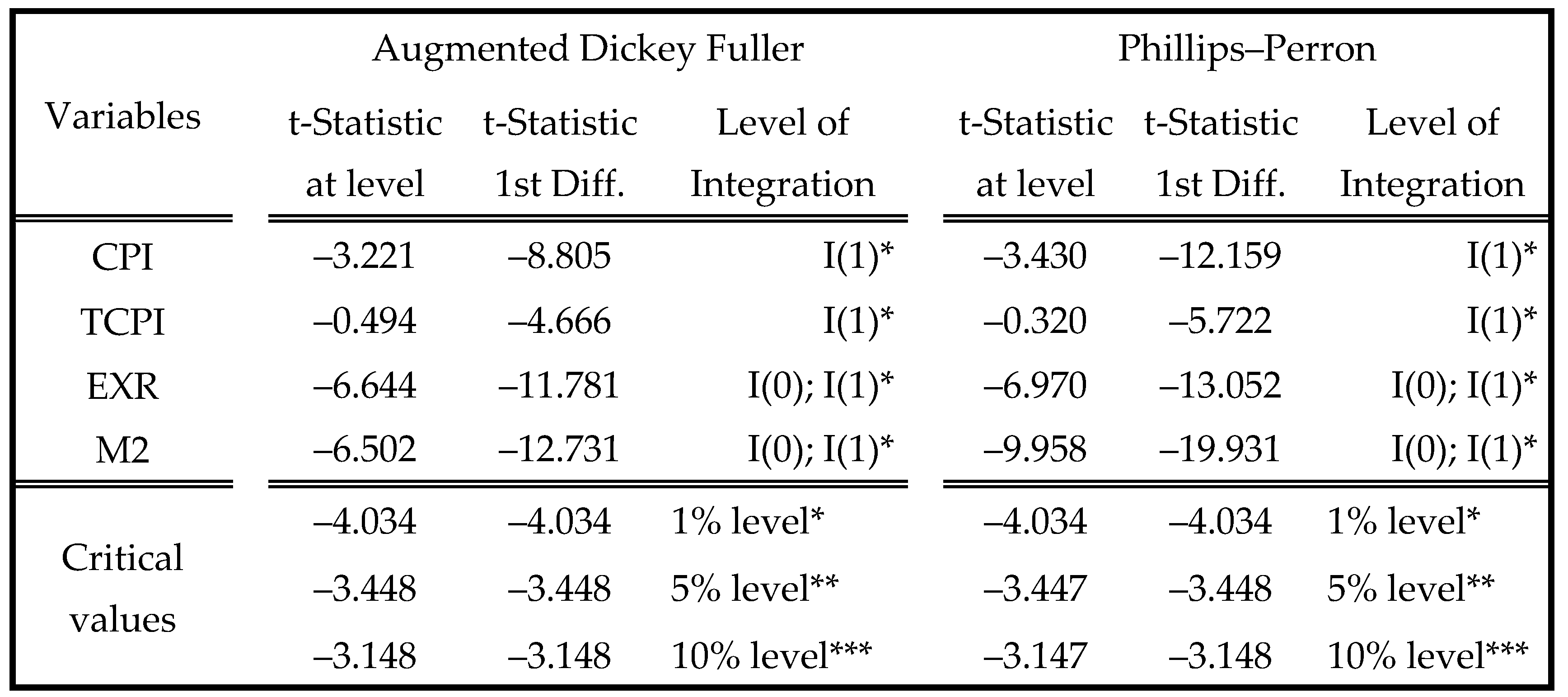
Figure 11.
ARDL bounds testing. Source: Author’s computation using STATA 14.2.
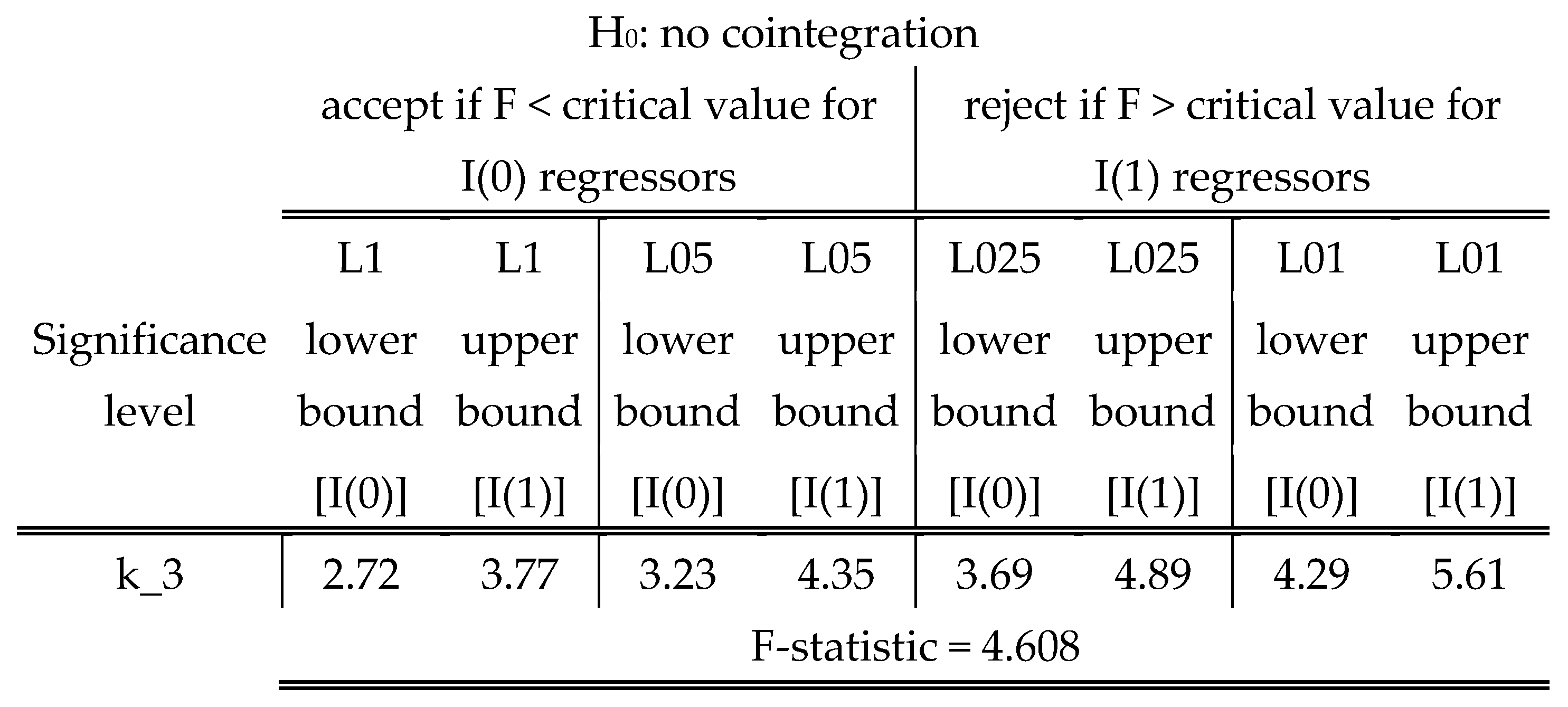
Figure 12.
Long run estimation results. Source: Author’s computation using STATA 14.2.
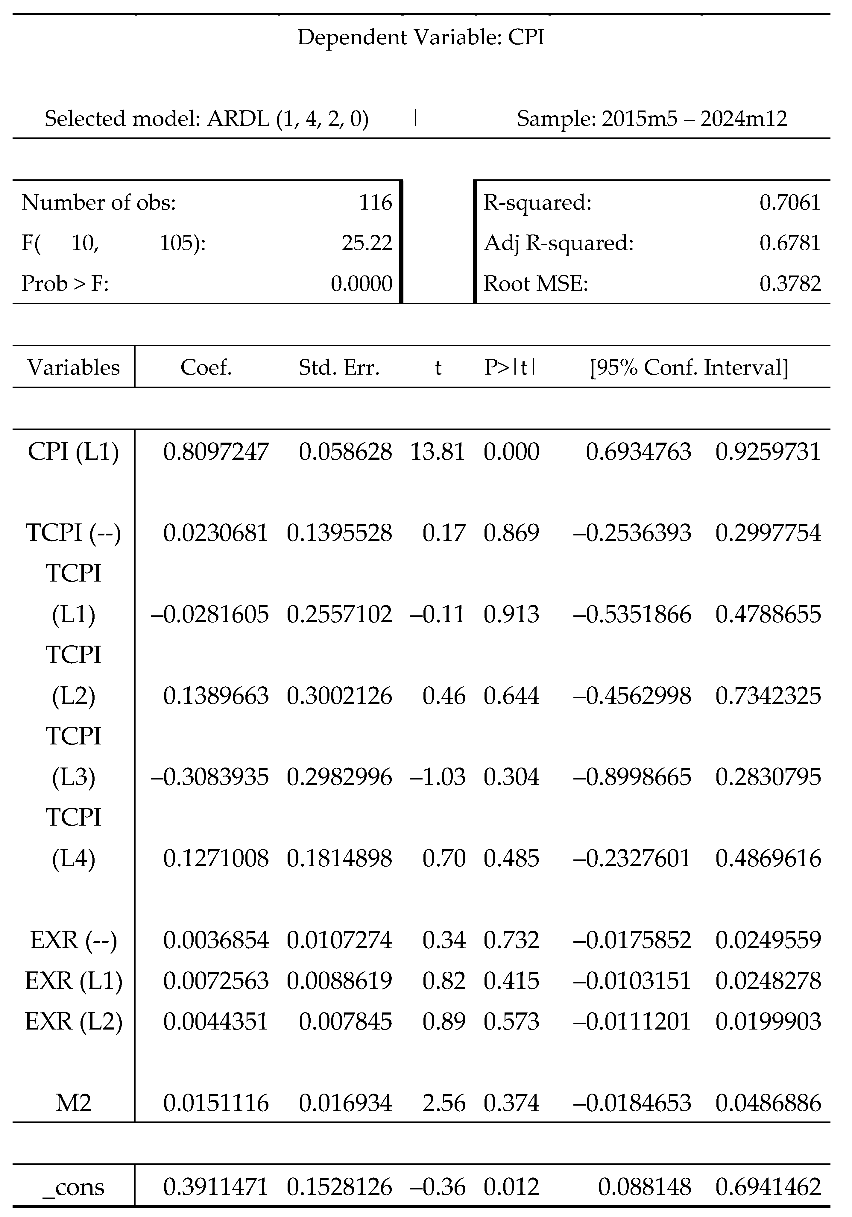
Figure 13.
Short run dynamics and error correction model results. Source: Author’s computation using STATA 14.2.
Figure 13.
Short run dynamics and error correction model results. Source: Author’s computation using STATA 14.2.
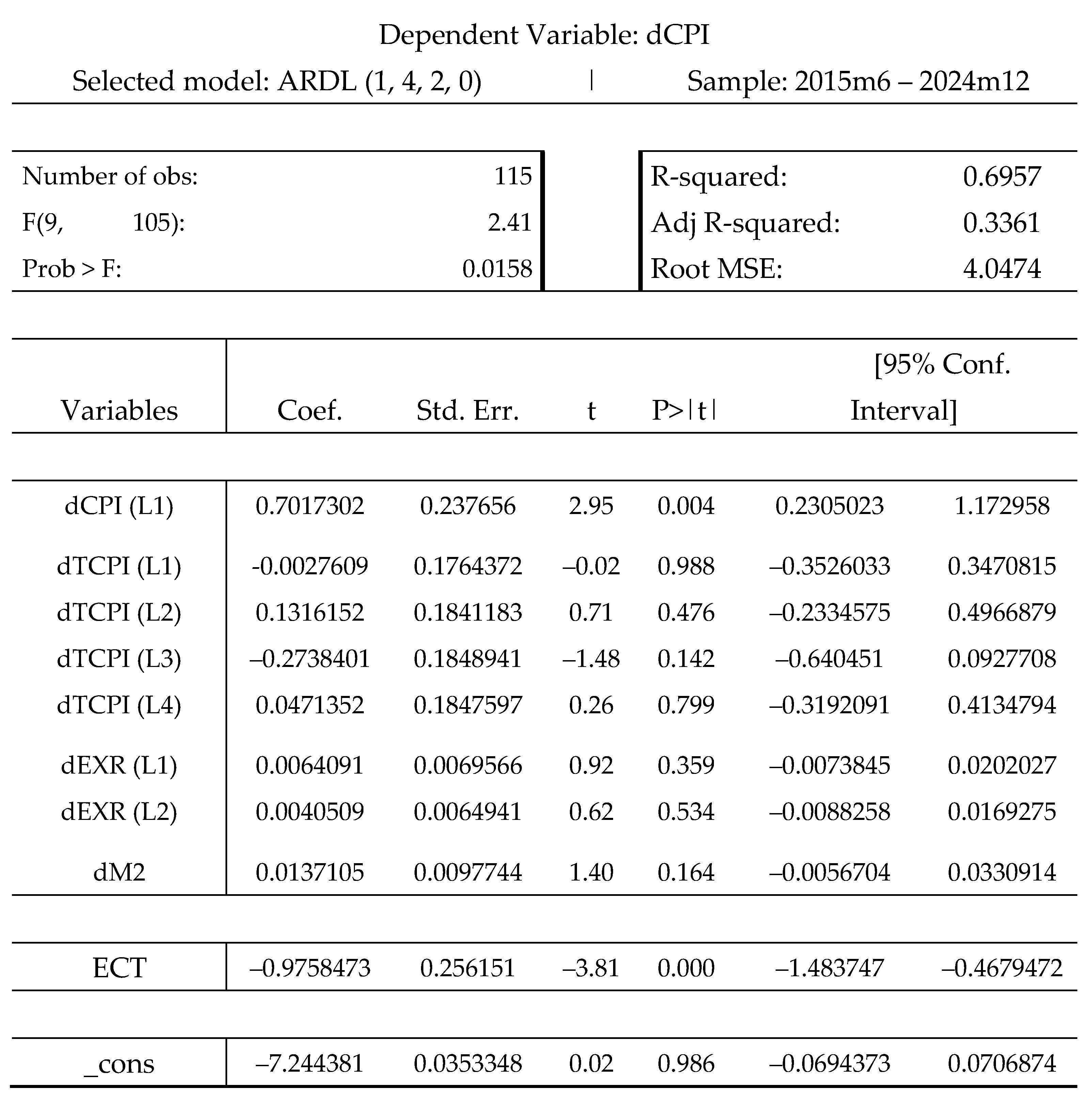
Figure 14.
Normality test. Source: Author’s computation using STATA 14.2.
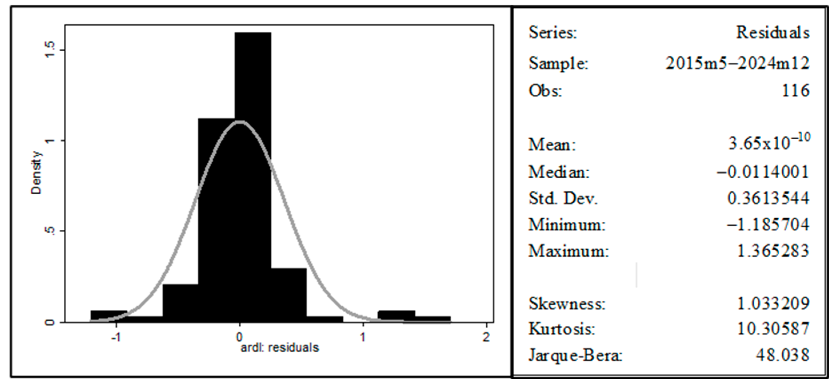
Figure 15.
VIF results. Source: Author’s computation using STATA 14.2.
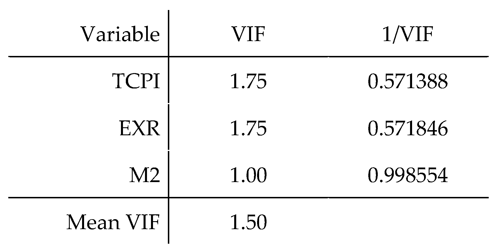
Figure 16.
Breusch-Godfrey test for autocorrelation. Source: Author’s computation using STATA 14.2.
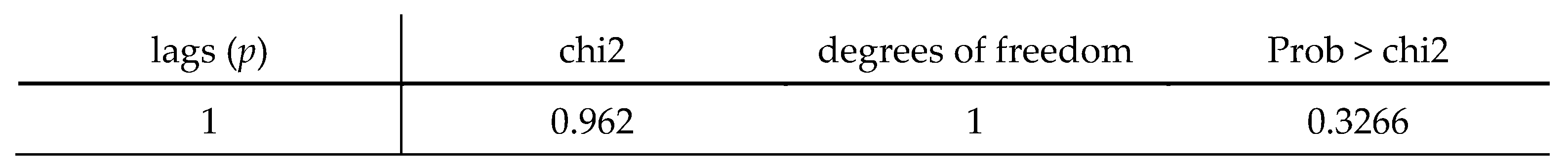
Figure 17.
White’s test for heteroscedasticity. Source: Author’s computation using STATA 14.2.

Figure 18.
CUSUM test results.
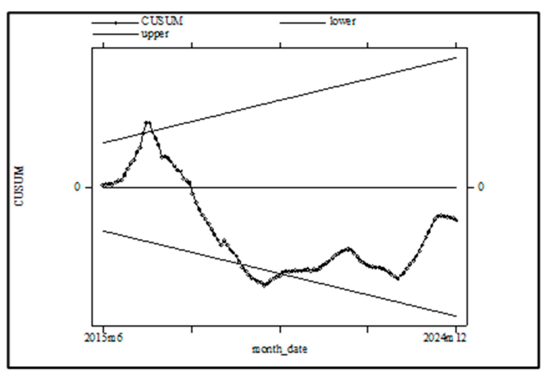
Figure 19.
CUSUM of Squares test results. Source: Author’s computation using STATA 14.2.
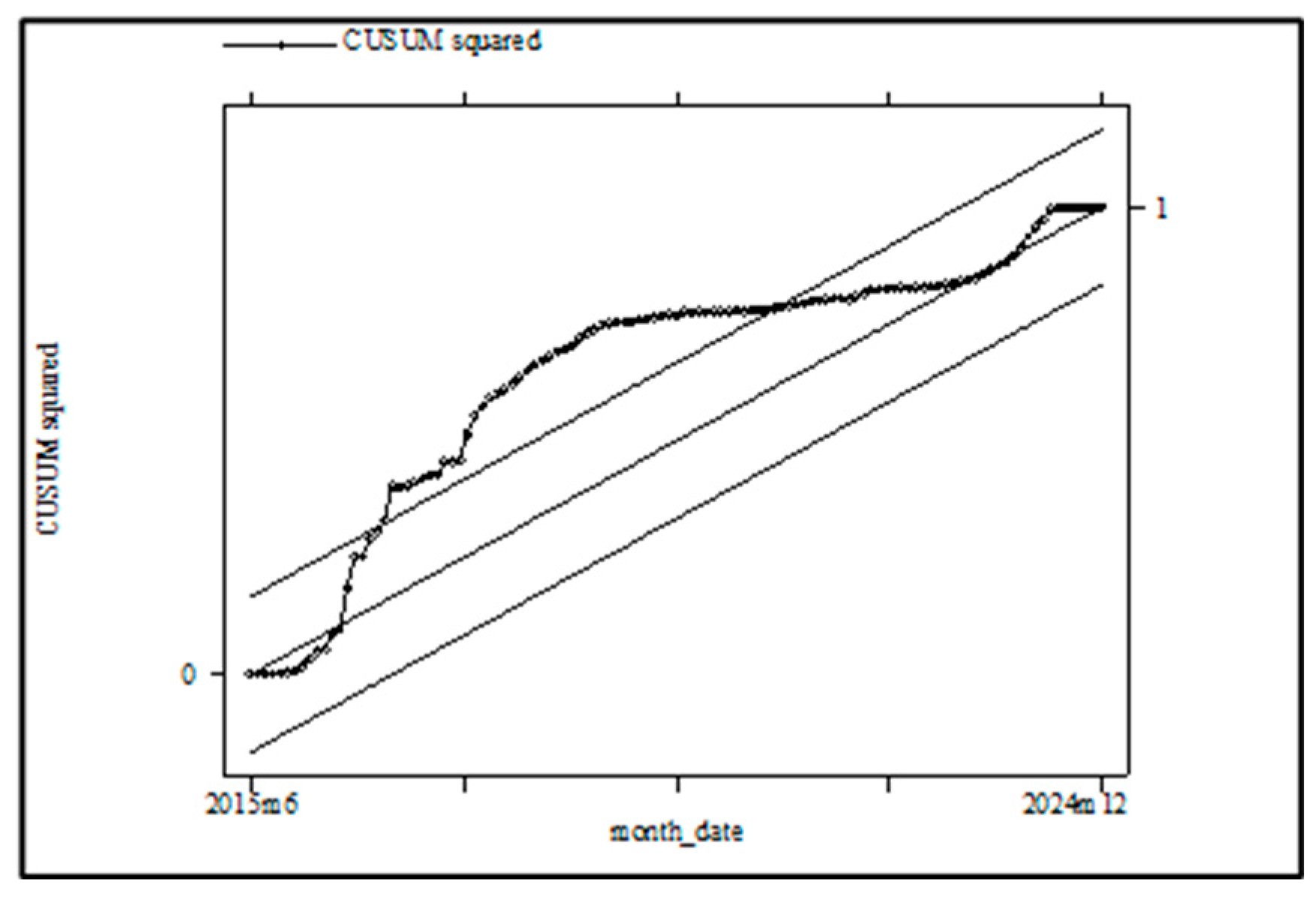
Figure 20.
Granger Causality Test. Source: Author’s computation using STATA 14.2.
Disclaimer/Publisher’s Note: The statements, opinions and data contained in all publications are solely those of the individual author(s) and contributor(s) and not of MDPI and/or the editor(s). MDPI and/or the editor(s) disclaim responsibility for any injury to people or property resulting from any ideas, methods, instructions or products referred to in the content. |
© 2025 by the authors. Licensee MDPI, Basel, Switzerland. This article is an open access article distributed under the terms and conditions of the Creative Commons Attribution (CC BY) license (http://creativecommons.org/licenses/by/4.0/).
Copyright: This open access article is published under a Creative Commons CC BY 4.0 license, which permit the free download, distribution, and reuse, provided that the author and preprint are cited in any reuse.


