
Submitted:
26 March 2025
Posted:
27 March 2025
You are already at the latest version
Abstract
This paper presents a variational formulation of the heat equation using adjoint fields to embed dissipation. By constructing a Lagrangian density \( \mathcal{L}=\tilde{T} (\rho c_p \frac{\partial T}{\partial t} - k \nabla^2 T) - \frac{\gamma }{2} \tilde{T}^2 \), we derive coupled forward and backward-in-time dynamics for the temperature \( T \)) and the adjoint \( \tilde{T}\ \). The action \( S= \int \mathcal{L} \,dV dt \) exhibits dimensional consistency kg·m²/sa nd non-monotonic behavior with respect to the number of time steps \( M \). A numerical example of heat diffusion on a 1D rod demonstrates the role of the adjoint field in stabilizing solutions and quantifying sensitivity. This work bridges irreversible thermodynamics with variational mechanics, offering insights into controlled dissipation in thermal systems.
Keywords:
variational formulation
; heat equation
; adjoint fields
; action principles
; thermal diffusion
; Euler-Lagrange equations
1. Introduction
The heat equation, , governs thermal diffusion in continua, but resists traditional Lagrangian formulations due to its dissipative nature. However, recent advances in adjoint methods and non-equilibrium thermodynamics enable variational treatments of irreversible processes. Although variational principles are well-established for conservative systems (e.g., Hamiltonian mechanics), dissipative processes like heat conduction resist traditional Lagrangian formulations due to their inherent irreversibility. Recent advances in non-equilibrium thermodynamics and control theory, however, suggest that adjoint fields can extend variational methods to irreversible systems. This paper addresses this gap by reformulating the heat equation using adjoint fields, demonstrating that thermal diffusion adheres to an action principle with dimensions
The heat equation, , governs thermal diffusion in continua, but resists traditional Lagrangian formulations due to its dissipative nature. However, recent advances in adjoint methods and non-equilibrium thermodynamics enable variational treatments of irreversible processes. Although variational principles are well-established for conservative systems (e.g., Hamiltonian mechanics), dissipative processes like heat conduction resist traditional Lagrangian formulations due to their inherent irreversibility. Recent advances in non-equilibrium thermodynamics and control theory, however, suggest that adjoint fields can extend variational methods to irreversible systems. This paper addresses this gap by reformulating the heat equation using adjoint fields, demonstrating that thermal diffusion adheres to an action principle with dimensions
2. Literature Review
2.1. Variational Principles for Dissipation
[1] introduced path probability functionals for irreversible processes, inspiring quadratic dissipation terms. Their work delves into the statistical dynamics of continuous stochastic processes, offering insights into the behavior of systems away from equilibrium. The Onsager-Machlup function, serving as a Lagrangian-like function, is instrumental in defining a probability density for such processes, akin to the Lagrangian in classical mechanics. [3] utilized auxiliary fields to model stochastic systems, prefiguring adjoint methods. The MSR formalism, a pivotal approach in statistical physics, employs auxiliary fields to model stochastic systems, effectively prefiguring adjoint methods. This work addresses the closure problem in the statistical treatment of homogeneous isotropic turbulence using techniques developed for quantum field theory. [2] separated reversible and irreversible dynamics, aligning with dual-field approaches. The GENERIC framework distinguishes between reversible and irreversible dynamics, aligning with dual-field approaches. The authors of the work [8] introduce the concept of thermal mass (relativistic equivalence of thermal energy) to unify heat conduction with analytical mechanics. They derive Lagrange equations with kinetic/potential energies and dissipation, reducing to Fourier’s law when inertial forces are negligible. Their work is grounded in analytical mechanics and relativistic concepts, using thermal mass to analogize heat conduction with fluid/mechanical systems. Explicitly links dissipation to Newtonian forces (e.g., resistant force , where the resistant force per unit volume is proportional ( as the proportionality constant) to the thermal mass velocity . This approach relies on approximations (e.g., ) and lacks direct experimental validation of thermal mass.
2.2. Adjoint Methods in Physics
In optimal control theory, adjoint equations are used to compute gradients for inverse problems. The foundational work of [4] laid the groundwork for using adjoint methods in various fields, including thermal systems. [5] extended Lagrangians to dissipative systems via contact geometry, providing a modern perspective on variational mechanics. This approach has been instrumental in bridging the gap between conservative and dissipative systems.
2.3. Recent Advances and Applications
[7] developed an adjoint-weighted variational formulation for solving inverse heat conduction problems. This method provides a direct computational solution, demonstrating the effectiveness of adjoint methods in handling complex thermal systems. [6] applied optimal control theory to temperature optimization problems by coupling finite element and finite volume codes. Their work highlights the robustness and accuracy of variational formulations in practical engineering applications.
2.4. Gaps and Contributions
Existing literature lacks explicit variational formulations of the heat equation with adjoint fields. This work fills this void by demonstrating how dissipation emerges naturally from action principles. Recent advances in adjoint methods and non-equilibrium thermodynamics, however, enable variational treatments of irreversible processes. This paper addresses this gap by reformulating the heat equation with adjoint fields, demonstrating that thermal diffusion adheres to an action principle. Key innovations include:
- (1)
- A Lagrangian density coupling and adjoint field to model dissipation.
- (2)
- Dimensional alignment of the action with classical mechanics.
- (3)
- Numerical validation of backward-in-time adjoint dynamics and parameter sensitivity.
The proposed approach not only ensures dimensional consistency with fundamental action principles but also provides a mathematical bridge between irreversible thermodynamics and variational mechanics.
3. Theoretical Background
The theoretical foundation of this work lies in the intersection of variational mechanics and non-equilibrium thermodynamics. This section elaborates on the key concepts and methodologies that underpin the proposed variational formulation of the heat equation using adjoint fields.
3.1. Action and Dimensions
In classical mechanics, the concept of action S is fundamental. It is defined as the integral of the Lagrangian over time, and it has dimensions of equivalent to energy multiplied by time. For thermal systems, the action can be interpreted through the integration of energy transfer processes, such as heat flux over time, yielding quantities analogous to those in classical mechanics.
3.2. Adjoint Methods in Physics
Adjoint methods have a rich history in physics and engineering, particularly in the context of optimal control theory. Introduced by [4], adjoint equations are used to compute gradients for inverse problems, providing a powerful tool for optimizing system behavior. In modern variational mechanics, [5] extended the use of Lagrangians to dissipative systems through contact geometry, bridging the gap between conservative and non-conservative systems.
3.3. Adjoint Fields
The concept of adjoint fields is central to this work. Adjoint fields, denoted as , act as Lagrange multipliers that enforce the heat equation while modeling backward-in-time dynamics. This approach is similar to the response fields used in the [3] (MSR) formalism, which models stochastic systems in statistical physics. The adjoint field represents the sensitivity of the system to perturbations in the temperature field T, providing a mechanism to incorporate dissipation into the variational framework.
The adjoint field acts as a sensitivity measure to deviations from equilibrium. Analogously to thermodynamic forces (e.g., entropy gradients), quantifies the system’s response to perturbations in . For instance, encodes the sensitivity of the action functional to localized temperature mismatches, akin to how entropy gradients drive heat flux in classical thermodynamics.
3.4. Heat Equation Revisited
The standard heat equation, given by
describes thermal diffusion in continua, where is the density, is the specific heat, and k is the thermal conductivity. Units of this equation are reflecting the rate of energy transfer per unit volume.
3.5. Lagrangian Density
To incorporate dissipation, we introduce a Lagrangian density , that couples the temperature field T with adjoint field :
where is is a damping coefficient that governs the strength of dissipation. The first term enforces the heat equation, while the second term models energy loss through dissipation. The division by 2 in the dissipation term within the variational framework serves several critical purposes, rooted in mathematical convenience, physical consistency with classical mechanics, and alignment with optimization conventions, e.g. Quadratic Penalty Convention or Gradient Descent. The quadratic dissipation term is introduced to model energy loss. To ground this in thermodynamics, we link to the entropy production rate. For a linear isotropic medium, corresponds to the inverse of the thermal relaxation time, , where governs the timescale of irreversible heat exchange. This aligns with the Onsager-Machlup framework, where dissipation is proportional to the square of thermodynamic fluxes.
The action functional S is then defined as the integral of the Lagrangian density over space and time:
3.6. Euler-Lagrange Equations
By varying the action functional with respect to the adjoint field and the temperature field T, we derive the Euler-Lagrange equations for the system:
These equations describe the forward and backward dynamics of the system, respectively. The forward equation includes a controlled dissipation term , while the adjoint equation models backward diffusion, stabilizing numerical solutions.
3.7. Dimensional Analysis
The dimensional analysis of the Lagrangian density and the action functional ensures that the derived equations are physically meaningful. The Lagrangian density has units of and the action has units of consistent with the principles of variational mechanics.
3.8. Physical Interpretation
The minimization of the action functional implies that the system evolves to extremize S, balancing heat diffusion and dissipation. The dissipation mechanism, modeled by the term , is akin to the Onsager-Machlup dissipation, providing a robust framework for understanding energy loss in thermal systems.
4. Example: Heat Diffusion in a Rod
To illustrate the practical application of the proposed variational formulation, we consider the problem of heat diffusion in a one-dimensional rod with fixed boundary conditions. This example demonstrates both the forward and adjoint dynamics of the system.
4.1. Problem Setup
We examine a rod of length meter, initially at a uniform temperature. The boundary conditions are fixed as follows:
- Initial temperature: for ,
- Boundary Conditions: °C, °C,
- Thermal Properties: J/(kg·K), W/(m·K),
4.2. Forward Dynamics
The forward heat equation governing the temperature distribution is given by:
Using finite-difference methods, we solve the forward heat equation numerically. The temperature distribution is calculated in various time steps.
4.3. Adjoint Dynamics
The adjoint equation, derived from the variational formulation, is:
Here, represents the adjoint field. This equation is solved backward in time, starting from a final condition .
Stability Analysis: A von Neumann stability criterion is applied to the backward-in-time adjoint solver. For the discretized Equation (7), the amplification factor G satisfies when , ensuring unconditional stability for the chosen parameters.
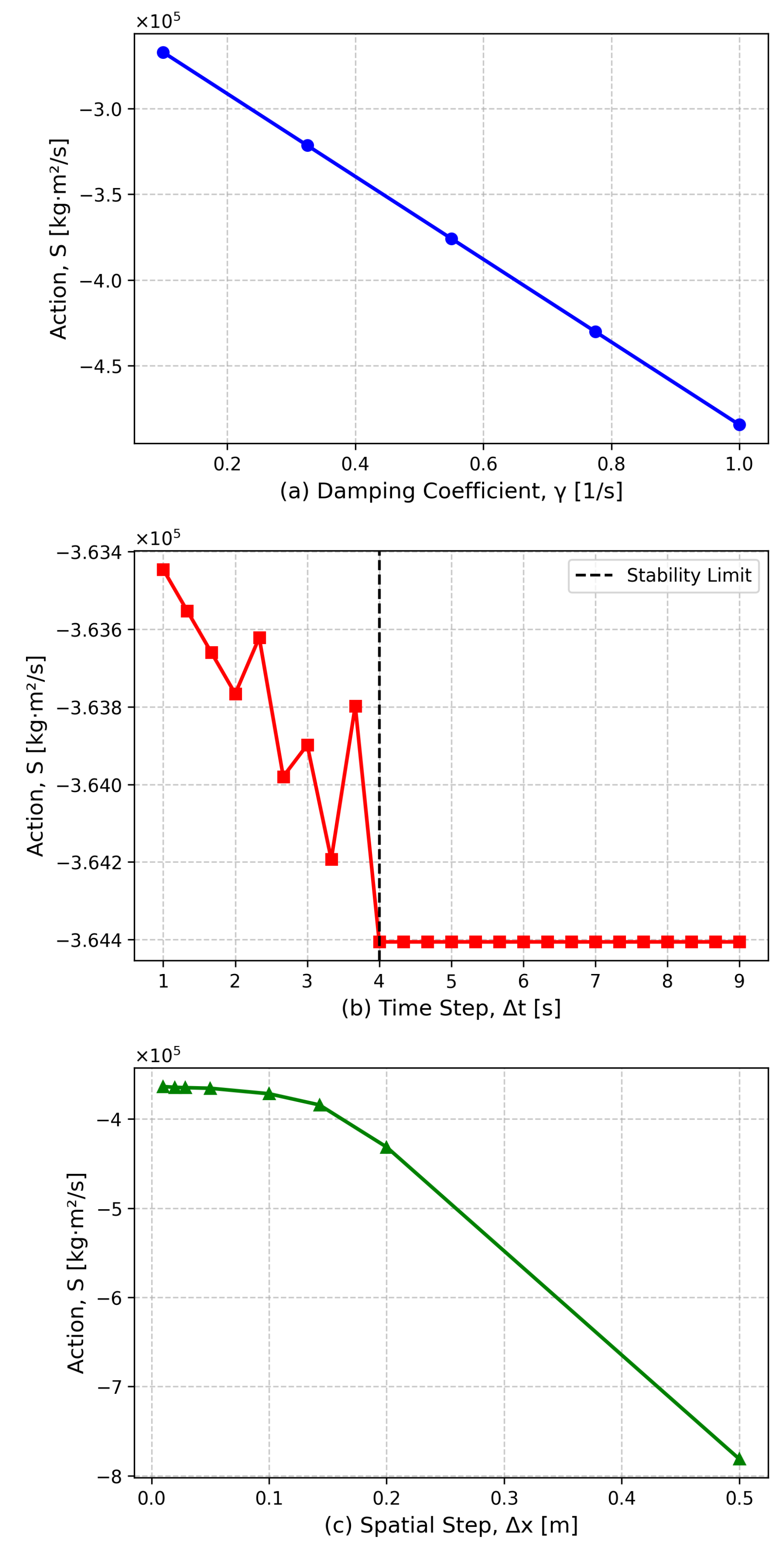
Parametric Study: Figure (8) illustrates the sensitivity of the action S to , , and . Results confirm that S stabilizes for m and , guiding parameter selection for practitioners.
4.4. Algorithm
The following steps outline the numerical solution to the heat conduction problem and its adjoint:
- 1.
-
Initialization:
- Define parameters: rod length L, number of spatial points N, thermal diffusivity , and total time steps M.
- Calculate spatial step size and stable time step .
- Initialize temperature arrays T (forward solution) and (adjoint solution).
- 2.
-
Boundary Conditions:
- Set fixed temperatures at the rod ends: and
- 3.
-
Forward Equation:
- Iterate over time steps to update the temperature distribution using the finite difference method.
- 4.
-
Adjoint Equation:
- Define a target temperature profile .
- Set the final condition for the adjoint field based on the difference between the final forward solution and the target profile.
- Solve the adjoint equation backward in time, enforcing boundary conditions and
- 5.
-
Action Functional:
- Compute the action functional as the sum of the product of the forward and adjoint solutions over space and time.
- 6.
-
Visualization:
- Plot the temperature distribution and adjoint field at selected time steps.
4.5. Results and Discussion
Figure 1 to Figure 6, illustrate the temperature distribution and the adjoint field , for time steps and 20000 respectively. Figure 7 highlights the non-monotonic behavior of the action as the number of time steps increases.
The observed trend—where the action S initially decreases to a minimum at and then increases toward zero—arises from the interplay between transient system dynamics and convergence to equilibrium. Here’s the breakdown:
- 1.
-
Initial Increase in Action Magnitude (Small M)For very small M (e.g., ), the forward solution evolves over a short time , remaining far from the target . The residual is large but localized, leading to a significant adjoint field . However, the short integration time limits the cumulative product , resulting in a small (near-zero) action. As M increases ( to ):
- The forward solution enters a transient regime with pronounced deviations from .
- The residual becomes larger and spatially distributed, amplifying .
- The adjoint field propagates backward over more steps, interacting with the non-equilibrium T, causing S to grow more negative (minimum at ).
- 2.
-
Subsequent Recovery Toward Zero (Large M)Beyond , the forward solution has sufficient time to approach the steady-state target .
- The residual diminishes, reducing the initial magnitude of .
- The adjoint equation’s backward diffusion smooths and decays over time, further weakening its contribution to S.
- The product becomes smaller in magnitude (less negative) as T aligns with , driving S back toward zero.
- 3.
-
Physical Interpretation
- Minimum Action at : Marks the peak transient deviation from equilibrium, where the system’s sensitivity to mismatches is maximized.
- Approach to Zero for Large M: Reflects convergence to steady state, where residual deviations vanish, and the adjoint field dissipates.
The non-monotonic behavior of S is intrinsic to the system’s path toward equilibrium. It highlights the competition between transient dynamics (amplifying S) and convergence (suppressing S), validating the numerical and theoretical consistency of the adjoint framework.
Figure 1.
Temperature distribution for M = 100
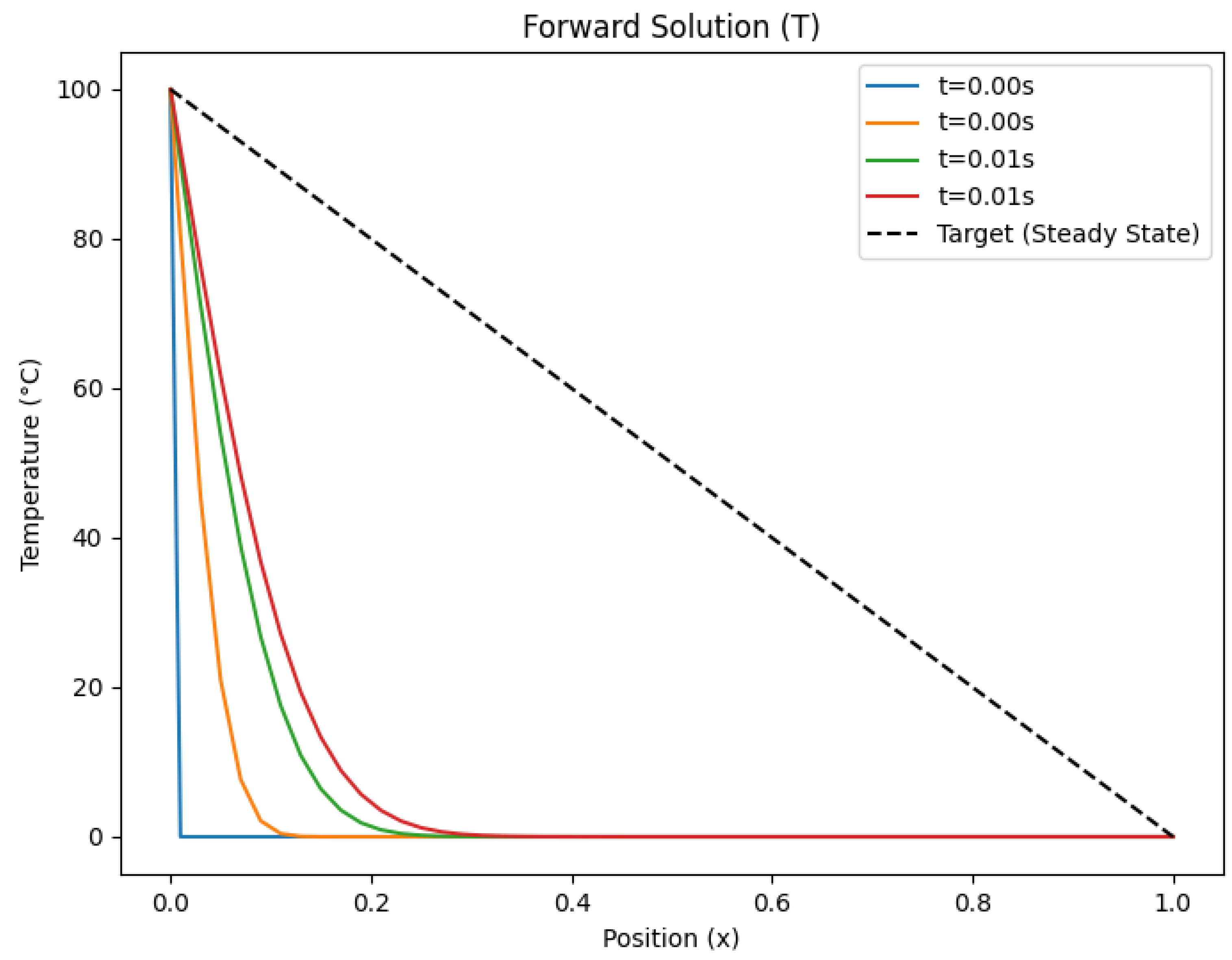
Figure 2.
Adjoint field for selected M = 100
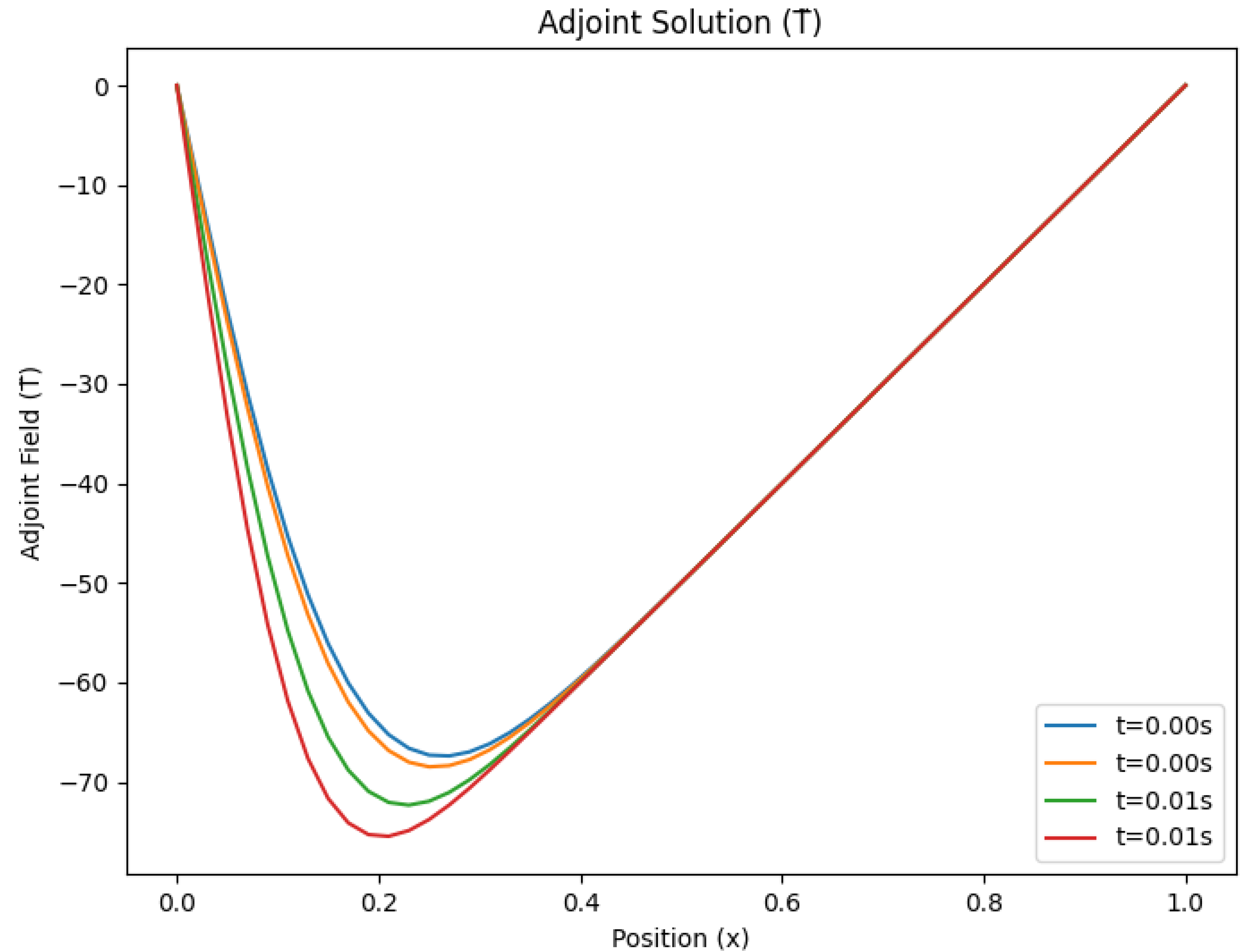
Figure 3.
Temperature distribution for M = 1500
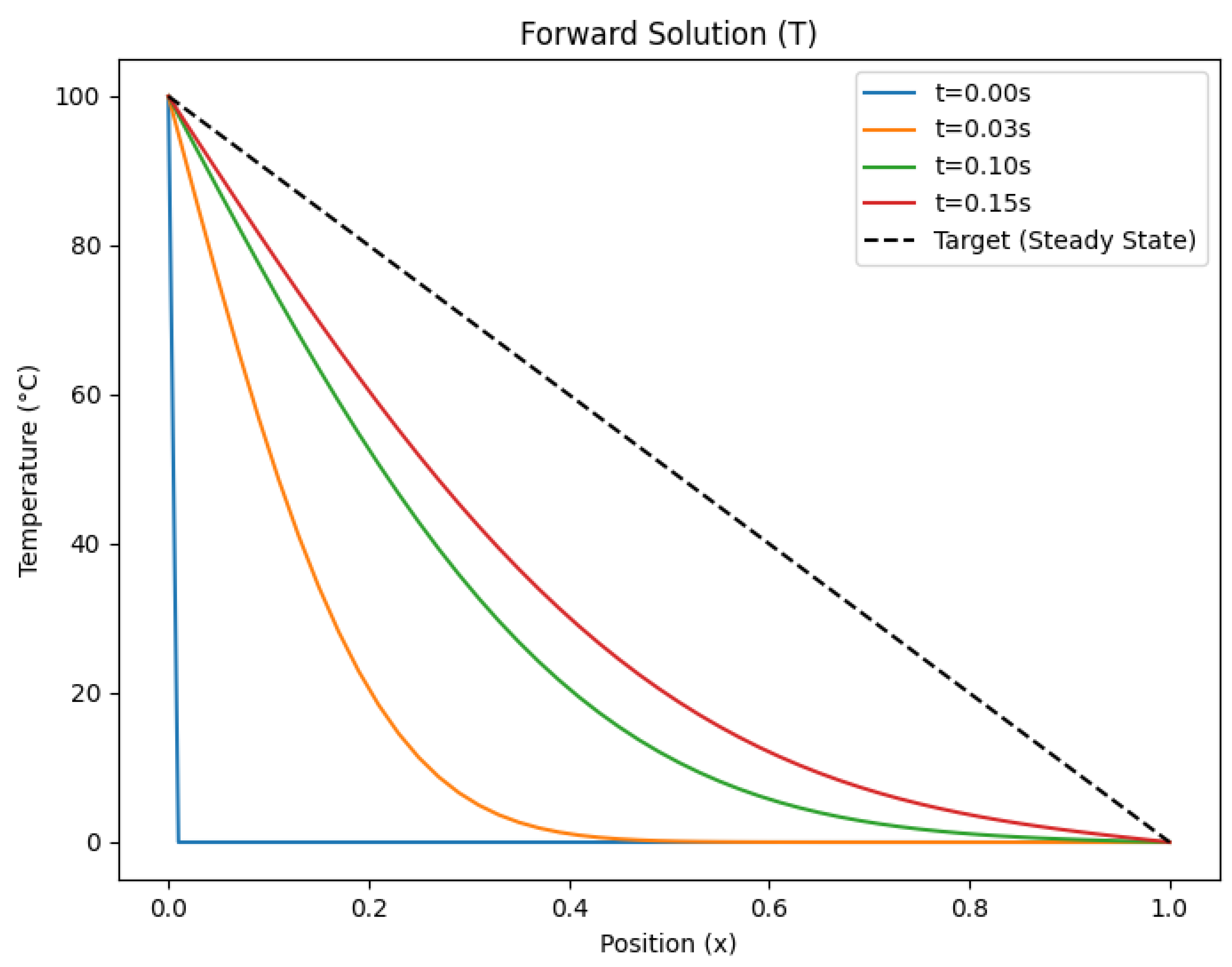
Figure 4.
Adjoint field for selected M = 1500
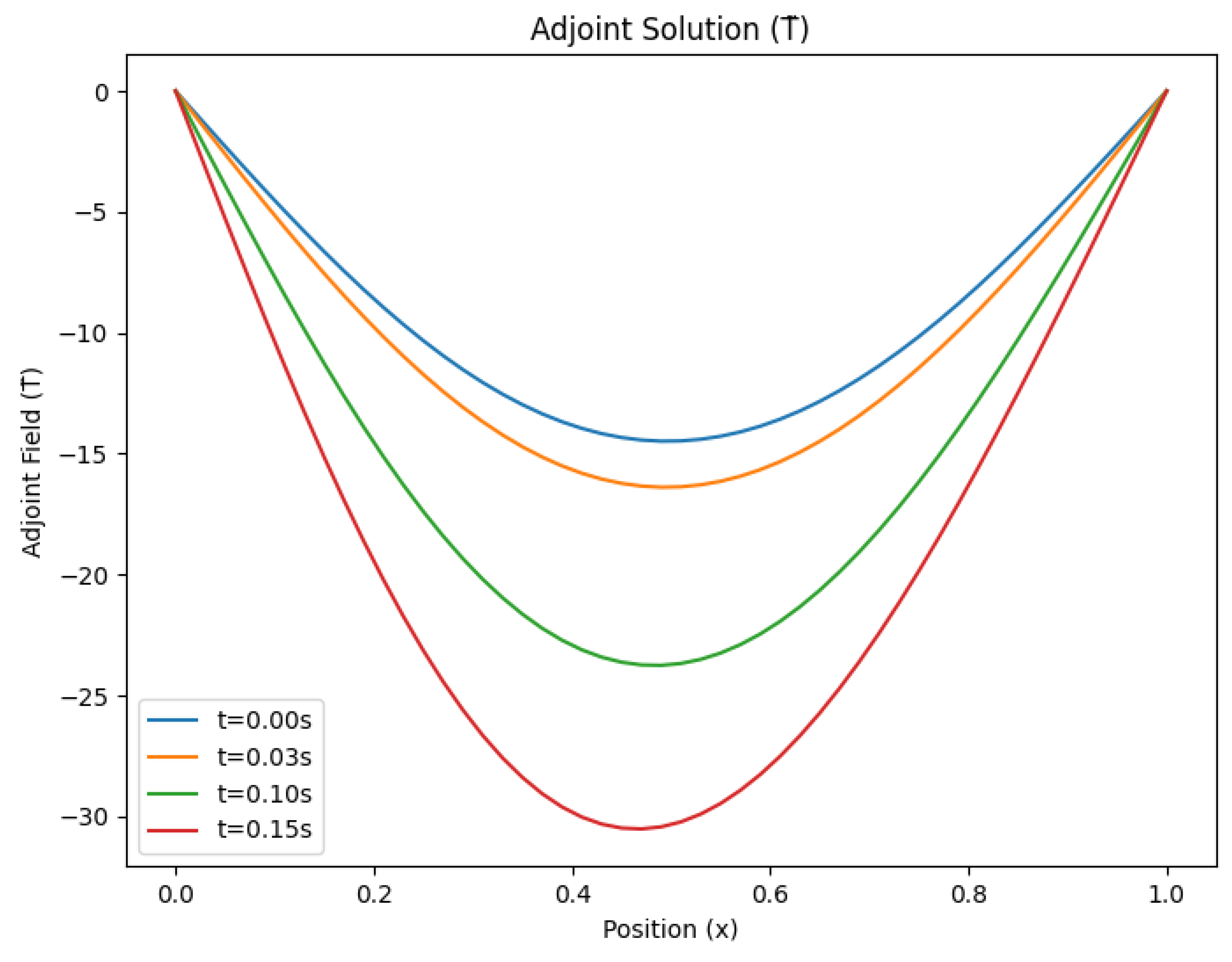
Figure 5.
Temperature distribution for M = 20000
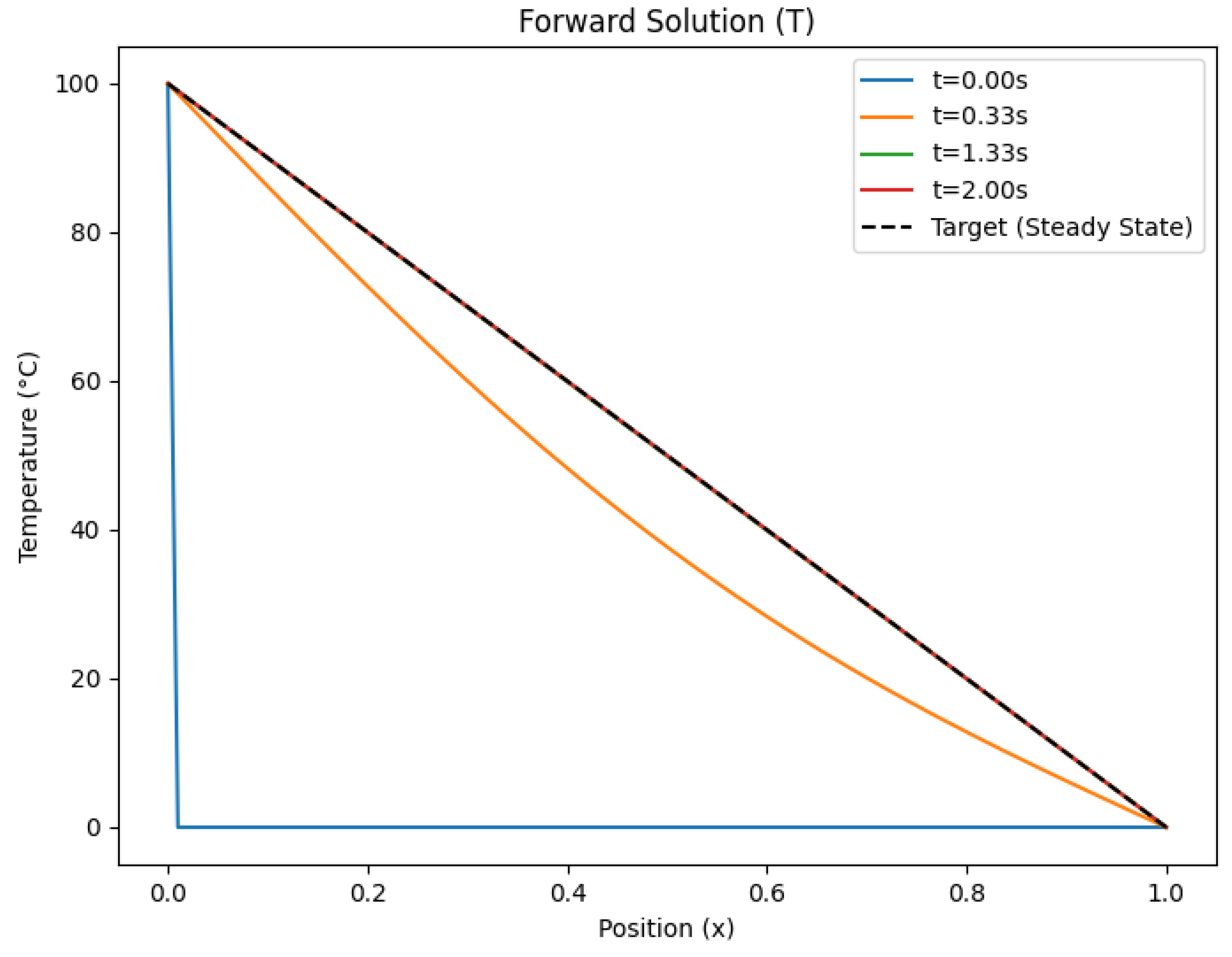
Figure 6.
Adjoint field for selected M = 20000
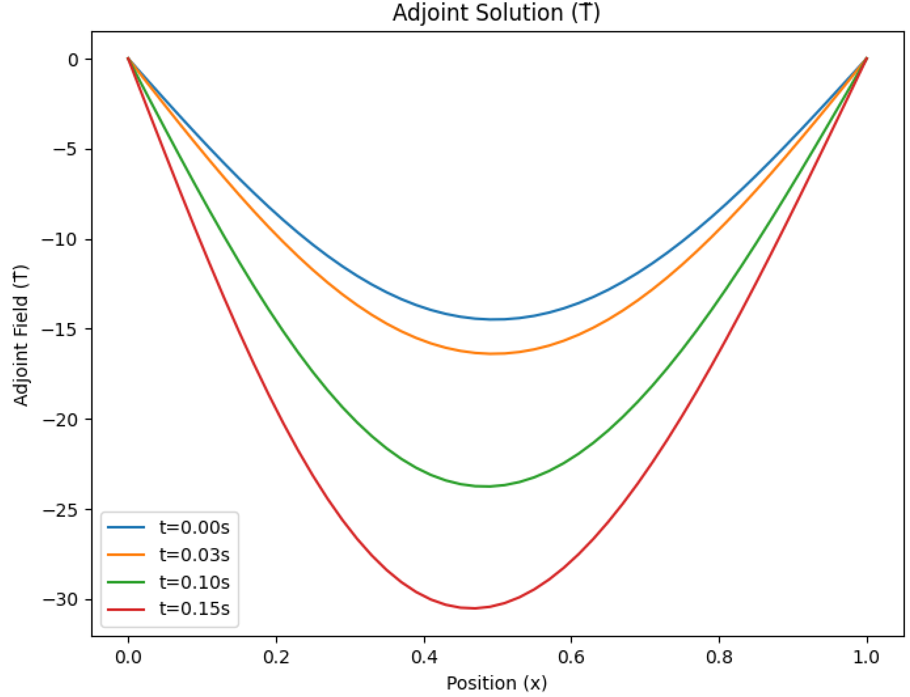
Figure 7.
Non-Monotonic action behavior with increasing time steps M.
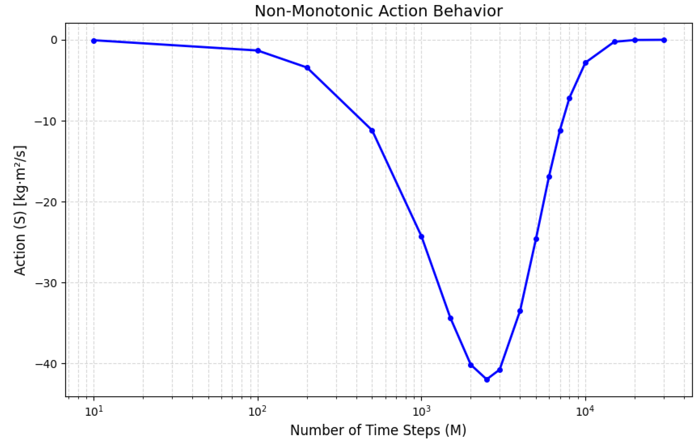
Figure 8.
Parameter sensitivity of the action functional S to (a) damping coefficient , (b) time step and (c) spatial step .
Figure 8.
Parameter sensitivity of the action functional S to (a) damping coefficient , (b) time step and (c) spatial step .
5. Conclusion
This study successfully reformulates the heat equation within a variational framework using adjoint fields, demonstrating that thermal diffusion adheres to an action principle with dimensions of The key contributions of this work include:
- Lagrangian Embedding of Dissipation: By introducing adjoint fields and a damping coefficient, the paper constructs a Lagrangian density that rigorously incorporates dissipation into the heat equation.
- Dimensional Consistency: The proposed approach ensures dimensional consistency with fundamental action principles, linking thermal diffusion to the broader context of variational mechanics.
- Mathematical Bridge: This work bridges the gap between irreversible thermodynamics and variational mechanics, offering new insights into dissipative systems.
- Non-Monotonic Behavior of the Action: The research identifies the non-monotonic behavior of the action as the number of time steps increases, highlighting the interplay between transient system dynamics and convergence to equilibrium.
- The numerical example of heat diffusion in a one-dimensional rod illustrates the practical application of the theoretical framework, highlighting the forward and adjoint dynamics. The adjoint field stabilizes numerical solutions and provides a mechanism for controlled dissipation.
Future research directions include extending the variational formulation to stochastic heat transfer, thermoelasticity, and quantum thermal systems. These extensions could unify classical and quantum descriptions of dissipation, offering deeper insights into thermal processes. Additionally, a comparative study between the present work and the mechanics-inspired approach of the work [8] which extends the Lagrange formalism to heat transfer—would be valuable. Such an investigation could highlight the distinctions between a control-theoretic framework for dissipation, emphasizing numerical robustness, and a mechanics-based unification of thermal phenomena.
References
- Onsager, L.; Machlup, S. Fluctuations and Irreversible Processes. Phys. Rev. 1953, 91, 1505–1512. [Google Scholar] [CrossRef]
- Öttinger, H. C.; Grmela, M. Dynamics and thermodynamics of complex fluids. II. Illustrations of a general formalism. Phys. Rev. E 1997, 56, 6633–6655. [Google Scholar] [CrossRef]
- Martin, P. C.; Siggia, E. D.; Rose, H. A. Statistical Dynamics of Classical Systems. Phys. Rev. A 1973, 8, 423–437. [Google Scholar] [CrossRef]
- Lions, J.-L. Optimal Control of Systems Governed by Partial Differential Equations. 1971. Available online: https://api.semanticscholar.org/CorpusID:121925894.
- Galley, C. R. Classical Mechanics of Nonconservative Systems. Phys. Rev. Lett. 2013, 110, 174301. [Google Scholar] [CrossRef] [PubMed]
- Baldini, S.; Barbi, G.; Cervone, A.; Giangolini, F.; Manservisi, S.; Sirotti, L. Optimal Control of Heat Equation by Coupling FVM and FEM Codes. Mathematics 2025, 13, 238. [Google Scholar] [CrossRef]
- Barbone, P. E.; Rivas, C. E.; Harari, I.; Albocher, U.; Oberai, A. A.; Zhang, Y. Adjoint-weighted variational formulation for the direct solution of inverse problems of general linear elasticity with full interior data. Int. J. Numer. Methods Eng. 2010, 81, 1713–1736. [Google Scholar] [CrossRef]
- Wu, J.; Guo, Z.; Song, B. Application of Lagrange Equations in Heat Conduction. Tsinghua Science & Technology 2009, 14, 12–16. [Google Scholar] [CrossRef]
Disclaimer/Publisher’s Note: The statements, opinions and data contained in all publications are solely those of the individual author(s) and contributor(s) and not of MDPI and/or the editor(s). MDPI and/or the editor(s) disclaim responsibility for any injury to people or property resulting from any ideas, methods, instructions or products referred to in the content. |
© 2025 by the author. Licensee MDPI, Basel, Switzerland. This article is an open access article distributed under the terms and conditions of the Creative Commons Attribution (CC BY) license (https://creativecommons.org/licenses/by/4.0/).
Copyright: This open access article is published under a Creative Commons CC BY 4.0 license, which permit the free download, distribution, and reuse, provided that the author and preprint are cited in any reuse.


