
Submitted:
29 March 2025
Posted:
31 March 2025
You are already at the latest version
Abstract
Research on abdominal aortic aneurysm (AAA) primarily focusses on developing a clear understanding of the initiation, progression, and treatment of AAA through improved model accuracy. High-fidelity hemodynamic and biomechanical predictions are essential for clinicians to optimize preoperative planning and minimize therapeutic risks. Computational fluid dynamics (CFD), finite element analysis (FEA) and fluid-structure interaction (FSI) are widely used to simulate AAA hemodynamics and biomechanics. However, the accuracy of these simulations depends on utilization of realistic and sophisticated boundary conditions (BCs), which are essential for properly integrating the AAA with the rest of the cardiovascular system. Recent advances in machine learning (ML) techniques have introduced faster, data-driven surrogates for AAA modeling. These approaches can accelerate segmentation, predict hemodynamics and biomechanics, and assess disease progression. However, their reliability depends on high-quality training data derived from CFD and FEA simulations, where BC modeling plays a crucial role. Accurate BCs can enhance ML predictions, increasing the clinical applicability. This paper reviews existing BC models, discussing their limitations and technical challenges. Additionally, recent advancements in ML and data-driven techniques are explored, discussing current state, future directions, common algorithms and limitations.
Keywords:
Abdominal aortic aneurysm
; Biomechanics
; Hemodynamics
; Fluid-structure interaction
; Boundary conditions
; Windkessel Model
; Machine learning
; Deep Learning
; Data-driven techniques
1. Introduction
An abdominal aortic aneurysm (AAA) is formed when the wall of the abdominal aorta weakens, leading to a localized balloon-like structure. By location, AAAs can be classified as supraceliac, juxtarenal, infrarenal and aortoiliac [1]. Infrarenal aneurysms are diagnosed when the diameter of the aorta exceeds 1.5 times of its normal size, approximately about 3 cm [2].The risk of aneurysm rupture increases with the diameter. For the aneurysms larger than 6 cm in diameter, risk of rupture ranges between 10% - 20% annually [3]. However, the diameter cannot solely predict the rupture risk, as clinical studies have documented ruptures in AAAs having diameter less than 5 cm [4]. AAAs develop often without showing any symptoms, resulting in severe cases of AAA being undiagnosed [2].
The aorta wall has thickness around 1.5 mm, composed of three primary layers (intima, media and adventitia), which include smooth muscle cells, collagen and elastin fibers embedded in ground matrix [5]. Their intrinsic mechanical properties enable the aorta to sustain loads at higher pressures. When pathophysiologically examined, an aneurysm can be described as expansion of the vessel wall due to thinning structure and the impact of mechanical stresses. Inflammation, oxidative stress, smooth-muscle-cell death and matrix degradation are the main causes of thin vessel wall structure [6]. Additionally, hemodynamic factors, primarily driven by blood pressure, flow velocity and resistance against flow, mechanically influence the vessel wall. A critical measure of this influence is the wall shear stress (WSS), which represents the frictional force exerted by blood flow along the vessel wall. While WSS acts tangentially to the direction of blood flow, blood pressure exerts perpendicular force to the vessel wall. These combined forces generate peripheral stresses which cause vessels to stretch and deform. The magnitude of these stresses changes throughout the cardiac cycle, making vessel deformation time dependent. Relative wall strain (RWS) quantifies these dynamic effects caused by the peripheral stresses [3].
Blood flow decelerates when it crosses an aneurysm due to the expansion in the cross-sectional area. This deceleration, along with the asymmetric structure and geometric distortions, results in disturbed flow patterns and vortex formation. The thinnest and innermost layer of the vessel wall (intima layer) is a membrane covered with endothelial cells reacting to the disturbed flow and WSS variations by the release of inflammatory markers [5,7]. Consequently, the low velocity regions with vortices and WSS variations promote the accumulation of the platelets in that area, potentially resulting in intraluminal thrombus (ILT) formation that might lead to degradation of the wall. Additionally, the areas of higher pressure indicate where the aneurysm may expand [8].
Numerous modeling and simulation studies have been commonly used in recent years to explore the hemodynamic and biomechanical properties of AAA, and the rupture risk. Rupture tends to occur in areas of low WSS and flow recirculation, rather than in regions of high pressure and WSS which conflict with earlier finite element analysis (FEA) based predictions [9]. AAA wall stress distribution is significantly influenced by aneurysm asymmetry and wall thickness variations. Models with variable wall thickness have shown up to a four-fold increase in peak wall stress compared to those with uniform thickness. Accuracy of wall thickness in computational models to predict AAA rupture risk emphasized by combining FEA and fluid-structure interaction (FSI) [10]. Patient-specific FSI models of AAA have proved that wall stress distribution and WSS are thoroughly affected by the interaction between blood flow and the arterial wall. These models show that high wall stress regions often align with complex flow patterns which carry higher risk in the context of rupture. Considering fluid dynamics via those interactions offers a more realistic simulation of in vivo conditions compared to models that do not include the flow effects [11].
Accurate modeling of AAA is clinically relevant due to its impact on predicting rupture risk, guiding surgical decisions, and improving patient outcomes. The integration of advanced modeling techniques into clinical practice helps avoid unnecessary surgical intervention and improves risk assessment. Rigorous biomechanical analysis is crucial for clinically relevant detection of AAA rupture risk via computational assessment. FSI models that incorporate patient-specific geometries with accurate wall thickness and boundary conditions derived from advanced imaging techniques such as phase-contrast MRI provide higher accuracy in predicting arterial wall stress and strain, which helps to recognize the smaller aneurysms with a high risk of rupture [12,13]. Integration of the machine learning algorithms to the geometric and biomechanical markers significantly enhances the classification accuracy of symptomatic and asymptomatic AAA. It is stated that the generalized additive model classifier achieved the highest accuracy using the combination of seven markers, demonstrating that integrating patient-specific geometric and biomechanical properties provides a more accurate rupture risk assessment than relying solely on the maximum aneurysm diameter [14]. Exceeding the traditional metrics such as maximum diameter [15] lies in bringing the interaction of hemodynamics, wall mechanics, geometric features into play with several modeling and simulation techniques. It is considered that integrating patient-specific data into these models will likely enhance the precision of AAA rupture predictions with the developing computational power and machine learning algorithms, and finally it will improve clinical decision-making and patient outcomes.
In summary, the recent advancements in computational techniques have enabled a more comprehensive understanding of the biomechanical and hemodynamic parameters associated with AAA rupture risk. In computational models, the use of realistic and sophisticated BCs plays a pivotal role in capturing the realistic physiological environment within the AAA. Accurate representation of these BCs at the inlet and outlet of the fluid domain, along with precise modeling of wall mechanics, is essential for enhancing the reliability of simulations. Such developments not only refine predictions of arterial stress and strain but also support the integration of emerging technologies, such as machine learning algorithms, into AAA analysis. These advancements bridge the gap between theoretical models and their practical applications in clinical settings, promoting a more personalized approach to patient care.
This paper provides a comprehensive review of the diverse range of BCs employed in AAA simulations, focusing on their application at the inlet and outlet of the fluid domain as well as wall conditions. Realistic BCs, such as the Womersley profile, Windkessel model, and fluid-structure interaction (FSI) techniques, are critical for accurate AAA simulations but are often absent in standard computational fluid dynamics (CFD) solvers due to their technical complexity and the need for a detailed understanding of the underlying clinical issues. This review aims to address these challenges by exploring the physical and mathematical principles behind these BCs, offering valuable insights to researchers. Additionally, key findings from the literature are summarized, highlighting the limitations and technical barriers of existing models. The paper concludes by discussing recent advancements in predicting hemodynamic and biomechanical parameters and disease progression through machine learning (ML) and data-driven techniques, with a focus on commonly used algorithms, their limitations, and potential future directions.
2. Computational Techniques for AAA Simulations
In the modeling of cardiovascular systems, various techniques have been developed. These can be categorized into low-dimensional (0D and 1D) [16,17,18,19] and high-dimensional (2D and 3D) [20,21,22,23,24] methods, based on the dimensionality of the simulation [18,25,26,27]. Low dimensional techniques are computationally affordable and suitable for capturing general flow features across the entire cardiovascular system [28]. Specifically, 1D models solve the Navier-Stokes equations along the arterial tree to predict the flow profiles and pressure waves as they propagate throughout the system [22,28,29,30,31,32,33]. High dimensional models can resolve detailed hemodynamic and biomechanical features in all spatial dimensions by solving governing equations in the solid and fluid domains. AAA has a unique and complex geometry with a wall thickness around 1.5 mm [34]. Therefore, 3D patient-specific simulations are essential to achieve high-fidelity hemodynamic and biomechanic predictions.
2.1. Patient Specific Modeling Approaches
Patient-specific modeling increases diagnostic and treatment accuracy by providing the examination adapted to individual anatomical differences. Non-invasive imaging methods such as magnetic resonance imaging (MRI) [35,36,37,38], time-resolved three-dimensional ultrasound (3D+t US) [39,40] and computed tomography angiography (CTA) are the typically used to extract patient-specific geometries for AAA [41,42,43,44,45]. When the non-invasive methods are inadequate to determine the patient specific geometry, invasive methods can be applied to provide more detailed information as imaging is performed in a more limited area. For instance, intravascular ultrasound (IVUS) is performed by inserting a catheter containing an ultrasound probe into a vein, allowing the probe to capture images within the vessel. The use of IVUS, especially in cases of AAAs, eliminates the use of contrast agents used in CTA. Patients who underwent CTA during endovascular repair (EVAR) procedures have shown deteriorating renal function over time [46]. Angiography methods are also important tools that can be used to model the geometric structure. For example, 3D rotational angiography (3DRA), which allows visualization of aneurysm structures of the order of 3 mm [47], and other traditional angiography methods can be applied for the aneurysms emerging in larger vessels such as the aorta.
Following patient-specific medical image acquisition in DICOM (Digital Imaging and Communications in Medicine) format, segmentation software such as MIMICS (Materialize, Leuven, Belgium), SimVascular, VMTK and ITK-SNAP reconstruct 3D models. Deep learning tools such as U-Net 3D [48], SegNet [49], 3DResUNet [50], attention-based residual U-Net (ARU-Net) [51] and Context-Aware Cascaded U-Net (CACU-Net) [52] architectures offer significantly faster segmentation process compared to traditional algorithms. The overall workflow of segmenting is represented in Figure 1 Lumen and AAA walls are segmented separately to differentiate between these zones. The range of AAA thickness is within 0.23-4.26 mm, with a median wall thickness of 1.48 mm [34]. The distribution of wall thickness on AAA is heterogeneous and changes from patient to patient. The geometrical structure of the wall has a significant importance to withstand the dynamic loads and careful segmentation of the wall is an important step in computational modeling.
Extracting comprehensive CTA images of the entire vascular network can introduce additional challenges. Moreover, large-scale image-based simulations of the entire arterial network are computationally demanding [16,54]. The common approach is to focus on a specific region of interest by cutting the aorta at certain boundaries. As illustrated in Figure 2, the region of interest is specified and truncated from the rest of the geometry by cutting the domain at the inlet and outlet boundaries during segmentation process [13,55,56,57,58,59,60,61,62,63]. Several segmented 3D AAA models are presented in Figure 3. The supraceliac region (SC) marks the boundary between the descending and abdominal aorta. Downstream from the SC, the aorta branches into the celiac trunk (CT), superior mesenteric (SM), left renal (LR), right renal (RR) and accessory right renal (ARR) arteries. The aorta segment below the renal arteries is called infrarenal region (IR), which bifurcates into the left central iliac (LCI) and right central iliac (RCI) arteries [37,64,65].
The placement of inlet boundary varies depending on the hemodynamic parameters under investigation. Some studies position the inlet by dividing the region of interest from the aorta at the SC [65,66,67], while others cut the aorta from the IR [10,68,69], depending on the type of aneurysm. The number of outlet boundaries varies based on the position of the inlet. When the inlet is positioned in the SC, the model typically includes at least six outlets, corresponding to the CT, SM, LR, RR, LCI and RCI arteries [37,64,65]. In contrast, placing the inlet in the IR reduces the number of outlets to at least two, located at LCI and RCI arteries. However, the number of outlets may increase if additional arterial branches supplying blood to organs are considered. For example, the CT bifurcates into the hepatic (H) and splenic (S) arteries, while central iliac arteries further divide into the external iliac (LEI and REI) and internal iliac (LII and RII) arteries. Therefore, the total number of outlets may vary, depending on the complexity and specific requirements of the simulation. In the following section, numerical analysis is explained by providing details of the governing equations, material properties and boundary conditions used in solid and fluid domains.
2.2. Analysis of the Fluid Domain
Computational fluid dynamics (CFD) is a numerical technique used to determine the main hemodynamic parameters, such as pressure and velocity fields of the overall fluid domain. In this technique, the following governing equations are numerically solved across a computational mesh to characterize the flow properties as given in Eq. (2.1) and Eq. (2.2).
Eq. (1) and Eq. (2) are continuity and Navier-Stokes equations, respectively. The term denoted by is the external force acting per unit volume of fluid. The parameters of and define the velocity vector, density and stress tensor of the fluid, respectively. The parameter of denotes the moving coordinate velocity [69]. In ALE formulation, is denoted as the relative velocity of the fluid with respect to the moving coordinate velocity [70,71]. Both pressure and shear stresses are calculated for determining the stress tensors as given in Eqn. (2.3).
defines the identity tensor, denotes the pressure and denotes the dynamic viscosity. The parameter of defines the shear rate and denotes the strain rate tensor given in Eq. (2.4).
Constitutive Models for Blood
As a first approximation, blood can be assumed as a Newtonian fluid with a constant dynamic viscosity across all shear rates (), and a constant mass density () [8,41,68,72]. However, at low shear rates, particularly below 100 s-1, the non-Newtonian behavior of blood becomes more prominent [73]. At low shear rates, the red blood cells (RBCs) aggregate and form rouleaux, which is rod shaped stacks of individual cells [73]. Rouleaux aggregation disperses as the shear rate increases, reducing the viscosity of blood. The resulting shear-thinning behavior caused by rouleaux disaggregation in blood plasma is the principal cause of the non-Newtonian behavior of blood. In numerical studies, shear-thinning behavior of working fluid, which is blood, can be modeled using several constitutive models. Viscosity functions with bounded and non-zero limiting values of viscosity can be written in the general form given in Eq. (2.5.)
In Eq. (2.5), are the asymptotic viscosity values at zero and infinite shear rates and is a shear dependent function, satisfying the following natural limit conditions given in Eq. (2.6) and Eq. (2.7).
Different choices of the function correspond to different constitutive models for blood, with material constants depending on the factors such as temperature, hematocrit, and plasma. In the literature, eight non-Newtonian models are commonly used to represent the shear-thinning behavior of blood: Carreau, Carreau-Yasuda [74,75,76,77,78], Casson, Quemada [79], Power, Cross, Simplified Cross, and Modified Cross [78,80,81,82,83,84,85,86,87,88], as summarized in Table A in Appendix A.
On the other hand, the behavior of RBCs cannot be fully characterized by viscous phenomenon because they can be regarded as fluid filled elastic cells [89]. Therefore, blood exhibits viscoelastic nature due to RBCs viscous shear thinning and elastic properties [90]. In addition, increasing hematocrit, which is the volumetric ratio of RBCs in blood, causes increasing viscosity of the blood and makes non-Newtonian behavior of blood more significant. However, as the shear rate increases beyond the low shear rate region, the shear-thinning characteristics diminish, and blood exhibits Newtonian behavior [73].
To account for the elastic nature of blood, the viscoelastic Oldroyd-B model is frequently implemented [91,92,93]. In that model, the stress tensor in the linear momentum equation is decomposed into viscous and elastic parts as [73,93]. The viscous part of the Oldroyd-B model can be Newtonian or shear-thinning [90]. The elastic part satisfies the following constitutive equation given in Eq. (2.8).
2.3. Analysis of Solid Domain
The finite element analysis (FEA) is a numerical method that allows the calculation of stresses and strains within the solid region to understand mechanical behavior of the solid structure under various conditions. The governing equation provided in Eq. (2.9) is numerically solved across a mesh created through the entire solid domain.
In Eq. (2.9), defines the solid stress tensor, defines the body forces per unit volume, and defines the structural displacements. By writing the stress variable in terms of strains using Hooke's law, the differential equation can be written in terms of displacements, as given in Eq. (2.10).
In Eq. (2.10), the stiffness tensor is defined as , the solid strains are defined as , and a linear correlation is defined between the stress and strain. However, in many cardiovascular modeling studies, the solid region to be investigated does not exhibit a linear elastic behavior [94]. Modeling the AAA tissue requires proper defining the mechanical properties of wall and ILT. The constitutive models of AAA wall are developed, calibrated and validated through tissue characterization experiments [95,96,97,98]. To fit stress-strain behaviors, uniaxial tensile tests are conducted using tissue samples gathered during surgery [94]. AAA wall tissue exhibits complex material properties due to its layered, fiber-oriented structure, including hyperelasticity (non-linear stress-strain behavior), viscoelasticity (time-varying response due to relaxation), and anisotropy (direction-dependent characteristics due to distribution of the collagen fibers) [15,99].
2.3.1. Constitutive Models for AAA Wall
As a first approximation, the aneurysm wall can be modeled as a single layer with linear elastic properties and isotropic medium characteristics using elastic modulus of 2.7 MPa, Poisson’s ratio of 0.45, and mass density 2000 [57,58,100,101,102]. The elastic modulus ratio for three-layered models of intima: media: adventitia is [103,104] with elastic modulus of 3.2, 4,8 and 1.6 MPa, respectively [105,106].
While linear elastic description can be applied for the healthy aorta or the aneurysm with low curvature [107], effective characterization of non-linear stress-strain properties of AAA wall depends on the tissue's hyperelastic nature [97]. Fitting the hyperelastic constitutive models to the experimental data enables to determine the model coefficients. Although collagen fiber number and orientation influence the mechanical behavior, modeling with isotropic strain energy function is common [39,56,77,89,108]. To improve modeling accuracy, constitutive models including the anisotropy are available, capturing the directional dependency of collagen fibers in the strain energy function [95,96,97,98,107,109,110,111].
- Hyperelastic and Isotropic Models
- Mooney Rivlin Model
In the literature, two- [13,108,112,113] and three- [106] parameter Mooney Rivlin models are commonly used to model non-linear stress-strain nature of AAA tissue and described as Eqs. (2.11), (2.12), and (2.13), respectively. The strain energy per unit volume is defined as
In Eq. (2.11), and are the material constants obtained by fitting the experimental data. is the first Green’s strain invariant, is the right Cauchy-Green strain tensor, and are the principal strains that determine the relative changes in length along each principal direction. is the ratio of deformed elastic volume to the undeformed volume of the material. For incompressible materials, due to zero change in material volume, that vanishes the last term of Eq. (2.11). is the material incompressibility term.
Considering the population averages, [99,114,115] material properties are determined as , for a single layered wall structure. However, the material constants show certain variations from patient to patient. The minimum, average, and maximum values of were reported as , respectively, while the corresponding values for as 117.6, 188.1, 355.7 [56,116]. These studies recommend using population-averaged values in simulations, as variations in the Mooney-Rivlin material constants have been shown to have a negligible impact on peak wall stress and wall displacement [107].
- Yeoh Model
Generalized Yeoh strain energy density function, is given in Eq. (2.14).
In Eq. (2.14), is the first invariant of the right Cauchy-Green strain, and is stress-like material parameters identified from experimental data [79,117]. For the second order Yeoh model, is defined as given in Eq. (2.15).
In Eq. (2.15), is used as , and is used as [94]. For the fifth order Yeoh model, the material values are calculated from planar biaxial experimental data as , , and .
- Hyperelastic and Anisotropic Models
To account for the anisotropic nature of the AAA tissue, Fung-type strain energy density function [118] is commonly used in the literature, which can be demonstrated as given in Eqs. (2.16), (2.17), (2.18), and (2.19).
In Eqs. (2.16) and (2.17), is a material constant related to the stiffness of the tissue, while , are the material constants depending on the specific tissue directions such as circumferential, longitudinal, and radial to capture anisotropy [107,119]. In Eqs. (2.18) and (2.19), and are the Green strains in circumferential and longitudinal directions, while are the principal stretches that determine the relative changes in length along two primary axes. By fitting the material parameters to the experimental data, the effect of anisotropic fiber orientations can be modeled. In addition to the Fung-type [120], the models offered by Holzapfel [98], Holzapfel and Gasser [121] and Choi and Vito [122] are commonly applied in literature. Most of the studies combine the isotropic and anisotropic strain energy density functions as given in Eq. (2.20) [94]
In Eq. (2.20), describes the energy stored withing the extracellular matrix, and demonstrates the effect of embedded collagen fibers.
- Constitutive Models for ILT
While ILT consists of two layers [123], with the inner layer forming about one-third and the outer layer about two-thirds of its thickness, modeling it as a single-layer elastic structure is common [56,108,124]. The elastic modulus of ILT is relatively lower than that of the wall. When ILT is initially formed, elastic modulus is nearly equal to 50 kPa, while it may reach up to 200 kPa due to the increasing rigidity of ILT structure with time [56]. Poisson’s ratio and mass density of ILT are generally used as 0.45 and 1050 , respectively. The tensile tests have shown that ILT tissue has an isotropic behavior [107]. To increase accuracy, nonlinear, hyperelastic and isotropic constitutive model for ILT developed by Martino et al. [123] can be used as given in Eqs. (2.21) and (2.22).
In Eqs. (2.21) and (2.22), and are the material parameters, and is the second invariant of the left Cauchy-Green stretch tensor. For the ILTs structure, and , and for inner and outer layers, respectively. By considering ILT as a single layer, material constants can be taken as and . Martino et al. [123] conducted a comparative study using various parameters and concluded that suggested mean parameters are sufficient, eliminating the need for patient-specific material constants.
2.4. Coupling of Solid and Fluid Domains: Fluid-Structure Interaction (FSI)
Modeling the AAA wall as rigid and stationary is common in literature due to its simplicity. In fact, the vascular layers are viscoelastic and subjected to large deformations by the blood flow generated loads. Conversely, the motion of hyperelastic walls alters the shape of fluid domain and hemodynamics within AAA, which necessitates a simultaneous blood flow and wall deformation treatment. Compared to flexible walls, rigid wall assumption obtains elevated WSS values up to 50% [125], underestimates the vortex development [109], and fails to predict pressure wave propagation [126,127]. Therefore, the mutual interaction among wall deformation and blood hemodynamics requires an FSI coupling at the aorta wall.
FSI is a multiphysics technique [71,125,128] that couples fluid domain to solid domain at the wall interface by exchanging the instantaneous fluid velocity and wall deformation values between domains. The domains do not overlap, and the two domains are coupled at the luminal surface by satisfying a set of physical interface conditions to ensure the compatibility of kinematics and tractions. The solid wall domain and ILT structure are modeled by finite-element analysis (FEA) by discretizing the momentum conservation given in Eq. (2.9), while CFD method is used to discretize the Navier-Stokes Equations given in Eq. (2.2) that resolves blood flow patterns. The solid domain moves through space and deforms under hemodynamic loads, altering the shape of the fluid domain and necessitating the use of the Arbitrary Lagrangian-Eulerian (ALE) formulation. The ALE description of fluid domain offers a moving coordinate system to simulate a non-stationary solution domain [129]. In ALE method, the mesh nodes may be displaced or be fixed as Lagrangian and Eulerian descriptions. With this freedom, large distortions within the fluid domain can be managed with more precision [129].
Solving the governing equations within such truncated solid and fluid domains, coupling the solutions through FSI procedure requires proper specification of the conditions at the boundaries of the domain, bringing concerns regarding the accuracy of the simulations. A high-fidelity, physiologically realistic modeling of AAA hemodynamics requires proper treatment to the conditions at the model boundaries. In Figure 4 and Table 1, boundaries are demonstrated for the fluid and solid domains. Appropriate specification of BCs at the inlet, outlets and walls of solid and fluid domains is essential to realistically couple velocity, pressure, stress distribution, kinematics, traction and wave propagation in the upstream and downstream vasculature. The typical modeling techniques commonly employed in the literature for these boundaries are investigated in the following section.
3. Modeling Boundary Conditions in Fluid Domain
The accurate prediction of hemodynamic parameters, such as pressure and flow rate, requires proper coupling of the AAA domain with upstream and downstream hemodynamics at the truncated inlet and outlet boundaries. Proper coupling ensures that the simulated AAA hemodynamics interact with adjacent arterial compartments, closely reflecting physiological conditions. Typically, the time-varying inlet flow rate given in Figure 5 is prescribed for the inlet located at IR [56,68,109]. To enhance model accuracy, patient-specific inlet flow rates can be obtained through Doppler ultrasonography or phase-contrast magnetic resonance imaging (PC-MRI) [130]. At each point, spatial variations in flow velocity can be incorporated through customized velocity profiles based on the time-dependent flow rate. These profiles can be employed as idealized (i.e., flat, parabolic or Womersley) or patient specific. Patient-specific inlet velocity profiles can be measured non-invasively using 4D-Flow MRI [13,130,131], a three-dimensional, time-resolved type of PC-MRI that measures and visualizes the temporal evolution of blood flow within a specific 3D volume [78,81,131]. Alternatively, the inlet boundary can be connected to a lumped description of the heart [132,133,134]. However, using time-dependent pressure at the inlet is not a common approach due to the invasive nature and low precision of intraluminal pressure measurement, which requires catheter placement inside the inlet artery segment.
Applying outlet boundary conditions (BCs) is typically more complex. One challenge is the clinical measurement of intraluminal pressure, which requires catheter placement [13]. However, a significant portion of the cardiovascular system, including capillaries and veins, are located downstream of the aorta and substantially influence the AAA hemodynamics. Acquiring in-vivo hemodynamic parameters at branching arteries using non-invasive techniques like magnetic resonance imaging (MRI) is challenging due to limitations in the spatial and temporal resolutions of the measuring devices and the physiological variations in patients during the imaging [135]. Van’t Veer et al. [136] compared non-invasive brachial cutoff blood pressure measurements with invasive catheter pressure measurements inside the AAA sac, reporting a 5% underestimation of systolic pressure and a 12% overestimation of diastolic pressure. The common approach, especially for geometries with one or two outlets, is to prescribe the time-varying pressure profile illustrated in Figure 5 at the outlets [34]. Various other techniques are available in the literature, including prescribed outlet pressure, flow-split method, lumped parameter models (e.g., 3-element Windkessel), and 1D distributed parameter techniques. The following section critically examines the common methods for defining boundary conditions, their applications, benefits, and drawbacks.
3.1. Inlet BCs
The time-varying flow rate at the inlet of an AAA can be integrated using customized velocity profiles, capturing spatial variations in flow velocity across the inlet section. The pattern of these flow rate waveforms is highly dependent on the inlet location. Depending on the requirements, the inlet can be positioned at the SC or IR locations. Figure 6 demonstrates the measured volumetric flow rates at SC and IR regions [54]. Patient-specific profiles measured from human aorta using 4D flow PC-MRI technique, offer a more accurate representation of individual blood flow patterns, while idealized profiles (e.g., flat, parabolic, or Womersley) can illustrate general flow behaviors and are often used when patient data is unavailable [13,131,137].
The 4D flow PC-MRI images capture blood velocity vector fields in multiple sagittal slices of a healthy human aorta [131,138,139] at various time instants during cardiac cycle. In this method, three-dimensional velocity maps at multiple time instants through the cardiac cycle are generated. The resulting pixel-based time-varying velocity vectors are imposed on each voxel at the inlet section [139]. Chandra et al. [13] proposed a technique for mapping velocity vector field data onto the inlet boundary of a patient-specific AAA model, acquired on the IR plane. The inlet velocity profiles derived from 4D flow PC-MRI have a boundary which changes shape, size, and position due to aortic expansion and contraction during systolic and diastolic phases. However, the cross section of the inlet boundary in the CFD models of AAA geometry remains fixed both temporally and spatially [137]. To address this mismatch, Schwarz-Christoffel mapping aligns the datasets. Directly measuring in vivo inlet velocity profiles is still challenging because of the mismatch generated by such cardiac motion and resolution of measuring devices [140,141]. Moreover, accessing complete high-quality patient-specific geometry and inlet profile data is not always possible due to limited imaging facilities [141,142].
Consequently, patient-specific velocity profiles are not commonly used as inlet BC in AAA simulations. Instead, many studies employ artificial profiles such as flat [58,143], parabolic [8,20,72,89,144,145] and Womersley [146,147,148,149]. Figure 7 shows the general pattern of the idealized velocity profiles supplied at the inlet of AAA models. Several studies have reported no significant difference between flow-MRI derived profiles and artificial ones [150].
The artificial velocity profiles are calculated from time-dependent, patient-specific volumetric flow waveforms represented in Figure 6 at the inlet section of the computational domain. Inlet flow rate waveforms are implemented to calculate the flat and parabolic velocity profiles using Eqs. (3.1) and (3.2)
where and are flat and parabolic velocities, is the time-dependent flow rate, and is the artery radius. As presented in Figure 7, the flat profile represents a uniform spatial distribution of velocity vector at the inlet interface. The parabolic profile, derived from Poiseuille’s equation, exhibits a parabolic spatial distribution.
These profiles cannot fully capture all the transient effects introduced by the physiological flow rate waveforms, including flow reversal regions 161]. In 1955, Womersley developed an exact solution for incompressible, Newtonian fluid flow through a cylindrical, rigid blood vessel. This solution considers a pressure gradient that is a periodic function of time which enables to capture reverse flow using the equations of motion and continuity. Figure 7 illustrates the velocity profile obtained by Womersley’s solution. To obtain the Womersley profile, it is necessary to write the time-dependent flow rate, , in the harmonic form as in Eq. (3.3)
In Eq (3.3), is the total number of harmonic coefficients [21,150]. ’s are the Finite Fourier Transform (FFT) coefficients of that flow rate, while the term corresponds to a steady pressure gradient [150]. Fourier series decomposition of the time-dependent flow rate should be performed to obtain the Fourier coefficients of the inlet flow rate waveform. The equation of Womersley velocity profile is given in Eq. (3.4) using inlet flow rate waveform.
In Eq. (3.4), and are the term of Womersley number and frequency, respectively. and are the Bessel function of the first kind of order zero and first, respectively [152]. In Supplementary Material, derivation of Womersley profile and MATLAB code are provided.
In Eq. (3.4), the first term on the right-hand side equals the steady Poiseuille equation while the second term is the harmonic [152]. Although the Womersley profile presents transient effects of physiological flow, especially for large Womersley number () values, its application and implementation as an inlet boundary condition can be challenging due to Bessel functions and imaginary numbers that it contains [153,154]. Consequently, most studies in literature utilize flat or parabolic profiles [155]. Current studies [21] show that Womersley profile can be obtained by providing sufficient entrance length, at least , and is enough for parabolic and flat profiles, respectively.
Helical flow patterns in aortic hemodynamics have been observed in thoracic aorta studies [138,156]. Blood flow forms helical patterns in the ascending and descending aorta, as well as in the upstream sections of AAA. This helical blood flow is a physiological characteristic where blood rotates and advances along the aortic axis [9,156]. These physiological helices potentially help maintain WSS within normal range [102,157], regulate flow, and protect vessels from thrombus deposition [158]. However, most AAA studies neglect the helical features of the incoming flow. To address this, Javadzadegan et al. [102,157] introduced a tangential velocity profile at the inlet to present the helical pattern of the incoming flow as presented in Eq. (3.5)
In Eq. (3.5) is the streamwise velocity, is the local tangential velocity component, and represent axial axis and undilated radius, respectively. is the spiral speed and is a constant that controls the magnitude of the spiral speed. In the literature, is typically defined as 1/6 for the aortic flows [159].
3.2. Outlet BCs
The purpose of the outlet BCs is to model the downstream vasculature that includes smaller arteries, arterioles, capillaries, venules, and veins that return blood to the heart [160]. Therefore, the choice of outlet BCs has significant influence on velocity and pressure fields, and wave propagation linked to the wall properties in 3D AAA simulations [161]. Different outlet BCs have been adopted to better produce in vivo hemodynamic conditions in the cardiovascular system including prescribed outlet pressure, flow-split method [162], lumped parameter models such as Windkessel, and resistance [24,25].
3.2.1. Prescribed Outlet Pressure
Prescribing specific pressure at the outlets is common in AAA simulations. Prior studies typically implemented zero-gauge pressure at the outlets by setting [163,164,165], and some current studies continue to use atmospheric pressure at the outlet for simplicity [147,149,166,167,168,169,170,171,172,173,174]. However, using zero-gauge pressure as an outlet boundary condition is insufficient for producing accurate flow and pressure features. This approach assumes that the outlet is open to the atmosphere, neglecting the effects of the posterior vasculature.
To avoid this unrealistic assumption, the common approach is prescribing a time-dependent pressure waveform instead [56,109]. However, invasively measuring pressure for branching arteries is challenging, so a general pressure waveform pattern demonstrated in Figure 5 is typically applied to all outlets. This method is frequently utilized in AAA simulations with an inlet at the IR region, where at most two outlets, LCI and RCI, exist [8,74,76,110,175,176,177,178,179,180,181,182,183]. However, this method is less suitable for AAA simulations with an inlet at the SC. In that case, the increased number of outlets from branching arteries between SC and IR segments brings complexities because the diameters and flow distribution among those arteries differs and the time-varying pressure data cannot be obtained simultaneously for each outlet. Reymond et al. [126,184] have obtained pressure waveforms for all outlet locations at ascending aorta using a 1D model and validated with in-vivo measurements to provide relevant physiological data. Furthermore, this method neglects the effect of arterial compliance, neglecting the downstream wave propagation. For a realistic simulation, matching the inlet flow waveform and outlet pressure distribution is essential and should be taken into consideration.
3.2.2. Flow-Split Method
The flow split method assigns specific flow rates to each outlet. These rates are determined through either formula-based calculations or direct in vivo measurements. Les et al. [37] reported the constant fractions of mean flows to each outlet. As shown in Figure 6a., the flow between SC and IR regions, called upper branch vessel flows (UBVF), is determined by subtracting the mean measured IR flow from the mean measured SC flow, corresponding to 1.31 and 3.51 L/min, respectively [37,64,65,185]. The remaining 2.2 L/min is distributed to upper vessel branches: 33% to the celiac trunk (CT), and 22.3% to superior mesenteric (SMA), the left renal (LR) and right renal (RR) arteries [37]. In the presence of accessory renal arteries, renal flow was divided proportional to the outlet area. CT is then branched into hepatic (H) and splenic (S) arteries, with the flow distributed equally between them [37]. The remaining IR flow is divided equally into the two common iliac arteries, LCI and RCI, and 70% of this flow is diverted to external iliac arteries, while 30% is sent to internal iliac arteries [37,72,133,146]. These percentages are tabulated in Table 2.
To calculate the flow rate split among the outlets, Murray’s law is used [186,187]. The application of Murray’s law to estimate the flow splitting at artery bifurcations has been investigated in the literature. Murray [188] formulated that in branching arteries, the flow in each outlet is proportional to the cross-sectional area of the bifurcated vessel. The general form of the Murrays law is given in Eq. (3.7).
In Eq. (3.7), is the flow rate at the outlet, is the total flow rate, is the radius of outlet, is the number of outlets. The exponent varies according to the arterial segment. Generally, it is considered to be 2 for the aortic segment [130,189]. Several studies have used an exponent of 3 for AAA [45,190,191,192]. However, specifying a fixed flow rate at each outlet is not a realistic boundary condition because the flow division changes during the cardiac cycle, especially in deformable wall simulations where the outlet area changes continuously [193]. Furthermore, this BC neglects wave transmission to downstream vasculature [160].
3.2.3. Lumped Parameter Model
To accurately model downstream vasculature at the outlets of the AAA, coupling the 3D computational domain with reduced order (0D or 1D) is a common practice [135,194]. 0D models, also called lumped models, are governed by a group of ordinary differential equations (ODEs) that assume spatially uniform distribution of blood pressure, , and flow rate, within cardiovascular compartments at any time instant [195]. In vascular systems, the most widely used 0D models are Windkessel (WK) models [161,196]. This method represents downstream vasculature using lumped-parameter networks similar to electrical circuits consisting of capacitors, resistors, and inductors to relate and [189]. The elasticity of arterial walls allows them to expand and store large volumes of blood, then relax and push that blood downstream. This phenomenon, referred to as arterial compliance (), is analogous to the behavior of a capacitor in an electrical circuit. Similarly, as blood flows downstream, the arteries bifurcate and form small-diameter capillaries and veins. The narrowing of arterial diameters generates significant peripheral resistance (, analogous to electrical resistance [197]. In larger arteries, inertial energy is stored and released due to acceleration or deceleration of fluid, which is expressed as an inertance (, analogous to electrical inductor. In this framework, blood flow and pressure are analogous to current and voltage, respectively. By applying Kirchoff’s voltage and current laws, ODEs governing the relationships between the and are derived, called as WK models [198,199].
WK models are classified based on the number of parameters or circuit elements ( and [199]. Figure 8 illustrates the most common types: the two-element, three-element, and four-element WK models [198]. In two-element WK model (WK2 or RC), , is related to and the distal pressure, , through a parallel combination of distal resistance ( and a compliance (. According to Poiseuille’s law, the resistance is inversely proportional to the fourth power of the artery radius, which makes the smallest arteries and arterioles the primary contributors to resistance in the cardiovascular system [199]. Consequently, the WK2 model accounts only for , which represents the resistance of the downstream vasculature caused by the small arteries and the capillary bed [79,200,201]. However, the WK2 model has limitations in accurately describing the pressure-flow rate relationship because it omits the resistance of larger arteries [198,199]. To address this, three- and four-element WK (WK3 and WK4) models were developed [44,198,202]. The WK3 model sufficiently replicates the realistic downstream pressure at the outlet sections that are consistent with experimental data. As a result, the WK3 model is commonly implemented in most hemodynamic simulations [142,155,198,203].
The WK3 model, often called the RCR model, consists of a proximal resistance () in series with a parallel arrangement of a distal resistance () and a compliance (). describes the resistance in the large ascending aorta, proximal to the AAA. Based on the wave transmission theory [198,204] it helps absorb incoming pressure waves and reduce artificial wave reflections [135]. In the literature, the proximal and distal resistances are sometimes denoted as and , respectively [133,135,205]. The sum of distal and proximal resistances is known as total arterial resistance, [37,197]. The WK3 model describes the relationship between and using the ODE in Eq. (3.8).
In Eq. (3.8), represents the pressure at which blood flow to smaller arteries and capillaries in the vascular bed ceases [135,206] and is typically assumed to be zero in the literature [130,133,189]. For each outlet , Eq. (3.8) can be written as
Figure 9 illustrates the 3D domain of AAA and arterial branches coupled with separate WK3 models at the outlets: S, H, SMA, LR, RR, LEI, LII, REI, and RII. This technique models downstream compartments of the arterial branch outlets in the 3D AAA domain. The parameters and are constant for each outlet and independent of spatial dimensions [189]. By using calculated in the 3D simulation and estimating WK3 parameters for each outlet , can be determined by solving Eq. (3.9). Various techniques for estimating WK3 parameters exist in the literature. When patient-specific and are available for each outlet, the least-square approach recently proposed by Romarowski et al. [207] is recommended. This method tunes the WK3 parameters to match measured in vivo patient-specific pressure and flow data [130]. However, both and are not always simultaneously available, as most branches are quite narrow to make in vivo measurements.
Some studies have taken the parameters from the literature data to avoid time-consuming parameter estimation process [155,208,209]. However, the parameters utilized should be carefully selected to match accurate patient pressure profiles because the values of WK3 parameters affect the hemodynamic parameters. In an uncertainty estimation study, Boccadifuoco et al. [189] reported that the waveform at the aorta outlet is mainly affected by capacitance, , while the is affected by . Consequently, iterative solutions or approximations are frequently utilized to tune WK3 parameters [210]. Several studies implemented formulations of 1D modeling for parameter estimation [32,37,72,135,137,197,204,211]. A good agreement has been reported between the simulated pressure and flow rates and the in vivo measurements [37,135,195,196].
In this technique, a global WK3 model is created as the 0D representation of the 3D computational domain, as illustrated in Figure 9. The global WK3 parameters ( and are defined at the inlet of the computational domain before calculating local WK3 parameters and for each outlet . An initial estimate of the global compliance (can be calculated by using the Eqs. (3.10) and (3.11) defined for total resistance in 1D modeling [130,133,135]
In Eqs. (3.10) and (3.11) are the mean, systolic and diastolic pressures, and is the time-averaged mean flow rate at the inlet [37,156,189,205,210]. The outlet pressure ( is taken as 4.4 kPa in some studies [135], while generally is considered as [39,45] In 1D simulations, the global compliance (, which is the ratio of a volume change, and the resulting pressure change, , is approximated as in Eq. (3.12).
In Eq. (3.12) are the maximum and minimum flow rates at the inlet, and is the difference between the maximum and minimum flow rates [135,196,211]. Les et al. [37] determined the system's global resistance and capacitance by iteratively solving for a pressure waveform instead of using Eqs. (3.10-12). This waveform was derived and further iterated as a function of the input SC flow waveform and initial estimation of Windkessel model parameters.
The global parameters ( and ) are used to calculate the local WK3 parameters at each outlet segment by utilizing Murray’s law [37,45,156,171,189,191]. Consequently, the total resistance and compliance at outlet can be calculated by using Eqs. (3.13) and (3.14), respectively.
In Eqs. (3.13) and (3.14), is the number of outlets, and are the area of outlet and sum of the area of all the aortic outlets, respectively. Table 2 presents the ratios of time-averaged mean flow rates diverted to sub-branches in the AAA section after the SC region. These values, reported by Les et al. [37], are widely used in WK3 parameter tuning for AAA simulations. The ratio between proximal and total resistance, is taken as 5.6% for most of artery segments, with the exception of renal arteries [5,22,37,39,45,133,197,212,213]. Renal arteries, connected to kidneys, have relatively low at the vascular beds, resulting in an ratio of [133]. Once the total resistance at the outlet is determined, the proximal and distal resistances can be calculated as
The calculation of local from the global WK3 parameters for the downstream compartments of CT, SMA, LR, RR, LCI, RCI, is summarized in Table B in Appendix B. The flowchart in Figure 10 summarizes overall process. Although these 1D formulations are frequently used in AAA simulations, still concerns exist regarding their applicability to detailed geometrical shapes and FSI simulations where the flow rate directed to each branch is not constant due to the arterial deformations [156].
To improve parameter estimation accuracy, various tuning methods have been developed, primarily for ascending aorta and aortic dissections. Jiang et al. [214,215] initially performed a CFD simulation with zero-gauge pressure imposed at all outlets, calculating flow rates and pressures to tune WK3 parameters. In subsequent rounds, they imposed WK3 with estimated values, continuing until the pressure difference was less than 5%. Several studies estimate local parameters through iterative ODE solutions to match physiological pressure distribution within specified systolic and diastolic limits for the AAA [39,212,216,217]. Some of the studies use general values like 120/80 mmHg [38,156,189,201,218,219]. Local WK3 parameters are adjusted until the desired waveform is achieved. Fonken et al. [39,213] measured patient-specific brachial blood pressure in supine position using a brachial cuff. Alimohammadi et al. [205] measured minimum and maximum pressures at all branches of type-B aortic dissection using a transfemoral flush angiographic catheter connected to a pressure transducer. To further improve estimation accuracy, Alimohammadi et al. [205] and Pant et al. [220] applied data assimilation technique and unscented Kalman filters, respectively.
Spilker et al. [221] and Bonfanti et al. [133] used reduced model tuning techniques to enhance initial guess accuracy, and various CFD simulation results have been used for further iterations to optimize local parameter fine-tuning. Li et al. [156] proposed a fast-estimating approach that eliminates the need for CFD simulation iterations. They initially obtain total resistances as input for each interface using 1D formulations, considering systolic and diastolic pressures as 120/80 mmHg. The local WK3 parameters are then optimized using the pattern search algorithm from MATLAB's global optimization toolbox.
After estimating the parameters, coupling of 3D with 0D domain is commonly done explicitly [222,223] or semi-implicitly. The derivative terms in Eq. (3.9) are typically discretized as in Eq. (3.16) by using backward Euler method [205]
In Eq. (3.16), [224]. To achieve appropriate coupling, the flow rate equality condition for the multiscale model at the interface, , must be satisfied [205]. The instantaneous pressure, , is calculated from Eq. (3.16) by using the flow rate for the current solver loop, and pressure and flow rate from previous time step, and , respectively [205,223]. The resulting pressure, is then supplied back to the 3D domain as the uniform pressure BC at the current time step. For implicit coupling, and is solved simultaneously in an iteration loop [225]. In explicit coupling, pressure is calculated at the beginning of an iteration by using the flow rate value from the previous time step.
WK3 coupling isn’t available on every solver. SimVascular offers coupled WK2 and WK3 [203], while it is not defined in other software. To make such a multidomain solution in OpenFOAM, heamofoam [226] can be used. To use WK3 BC in ANSYS, a user defined function (UDF) should be created to couple two domains. For CFX, Fortran subroutine can be defined [205,218]. In some studies, 3D-0D coupling is not performed. In several studies [42,227,228], time-dependent pressure waveform has been calculated through WK3 and applied them as prescribed pressure BC at the outlets.
3.2.4. Resistance BC
To relate the flow rate and the pressure at the outlets of the computational domain, some studies prefer to use resistance BC due to its simplicity [24,78,190,229]. In this technique, the resistive property of the downstream vasculature is imposed by a resistance parameter, while the compliance of the arteries is neglected with Eq. (3.17).
In Eq. (3.17), and are the resistance, time-dependent pressure and flow rate at the outlet, is the reference pressure related to the venous pressure. is calculated by distributing the global resistance calculated from Eq. (3.10) into branch arteries with Eq. (3.13). However, resistance BC is not commonly preferred BC in AAA simulations since it severely impacts wave propagation phenomena [160,230].
4. Modeling Boundary Conditions in Solid Domain
4.1. Inlet and Outlet of the Wall
The branch arteries of aorta produce a tethering effect on the AAA. To model this effect, zero rotation and translation conditions are imposed at the inlet and outlet of the wall domain [10]. To further improve the accuracy, Scotti et al. [69] specified 5% axial stretch on these boundaries [231] since the artery walls are physiologically under tension.
4.2. External Wall Boundary
The intra-abdominal pressure imposed by surrounding tissues and organs on the outer surface of the AAA wall requires consideration [232]. Most studies, however, assume a free stress condition with zero pressure on the external AAA wall. This boundary condition can lead to non-physiological wall motion patterns [193], causing several researchers to use a constant intra-abdominal pressure of 12 mmHg [69]. Crosetto et al. [233] introduced a Robin condition which requires appropriate model parameters through curve fitting to the empirical data. Similarly, Moireau et al. [234,235] developed a BC along the outer wall of thoracic aorta (TA) incorporating a viscoelastic term to account for surrounding tissue and organ support.
4.3. FSI Boundary: Coupling Solid and Fluid Domains
FSI modeling can be performed using several numerical approaches: one-way uncoupled [13], one-way coupled [66,236], and two-way coupled, both explicit and implicit [113]. In the one-way uncoupled method, intraluminal pressure load is supplied to the FSI interface, and only solid mechanics equations are solved in the wall domain, without feeding fluid domain with the pressures obtained by solid domain. In two-way coupled methods, solid and fluid domains are simulated simultaneously, interacting through the FSI interface. Comparative studies [236] showed that one-way FSI technique overestimates pressure, WSS, and strain in the fluid domain while underestimating the von Mises stress and displacement. As shown in Eqs. (4.1) -(4.3), three conditions must be met at FSI boundaries: solid and fluid domain displacements must be compatible, boundary tractions must be in equilibrium, and fluid must follow the no-slip condition on the FSI boundary surface.
In Eqs. (4.1)-(4.3), and are displacement vectors, stress tensors and boundary normal vectors at the FSI boundary for solid, s, and fluid, f, domains. In two-way explicit coupling, information exchange among fluid and solid domains occurs explicitly, without iterations within each time step. To obtain converged results, small steps are required. In two-way implicit coupling, the fluid and solid equations are solved simultaneously at each time step, iteratively exchanging information until convergence. While this method requires high computational memory and excessive computational time, it is necessary to reach convergence for improving accuracy.
5. Important Post-Processing Indices
Hemodynamics inside an aneurysm sac can be quantified by several wall shear stress (WSS) descriptors such as time-averaged wall shear stress (TAWSS), oscillatory shear index (OSI), endothelial cell activation potential (ECAP) and relative residence time (RRT). Mathematical definitions of these descriptors are given in Eqs. (5.1)-(5.4) [237,238].
where and are the cardiac cycle period and the wall shear stress, respectively.
Several studies also reported a correlation between recirculation zones and WSS descriptors. The utilization of vortex fields may afford a more comprehensive understanding on ILT development and rupture mechanism, compared to WSS descriptors [239,240]. In the literature, vortex structures are commonly quantified by , , , (swirling strength) criteria [241,242] and rortex [243]. The equations for vortex identification criteria are given in Appendix C.
For the AAA wall, principal wall stresses, Von Mises stress and wall displacements are critical parameters. Von Mises stress, based on three principal stresses, is a measure of failure prediction as given in Eq. (5.5).
In Eq. (5.5), are the principal stresses, is the uniaxial failure strength of the wall [34]. The term on the left-hand side is the square of the Von Mises stress. Peak wall stress (PWS) is a critical indicator of rupture, occurring when the AAA wall strength is insufficient to withstand the PWS [244].
6. Recent Findings
To accurately simulate the AAA hemodynamics and wall mechanics, researchers have developed and implemented different techniques over a quarter century. Starting from the axisymmetric geometries supplied with simplified boundary conditions and material properties, in silico investigation of the AAA development and rupture characteristics has reached patient-specific geometries with realistic boundary conditions, enhancing the reliability of predictions. Intense research has accomplished to couple different computational domains solved by various methods, such as CFD and FEA at the wall interface by implementing FSI technique, and different dimensions such as 0D and 3D. Increasing use of medical imaging techniques such as CT, MRI and 3D ultrasound enables the extraction of patient-specific geometries with accurate wall thickness distribution with eliminated prestress that ensures precisely capturing the anatomical features of AAA. Utilization of the 4D flow MRI and angiographic catheters enable to provide time-dependent patient-specific inlet velocity profiles and outlet pressure waveforms, respectively. With the help of biaxial and uniaxial tissue tests, accurate constitutive models with patient-specific material constants have been developed.
The utilization of 4D flow MRI inlet velocity profiles is common in the thoracic aorta (TA) studies [81,130,138,142,217], while the implementation of artificial velocity profiles developed from patient-specific inflow waveforms at SC or IR regions is standard practice in AAA simulations. Chandra et al. [13] obtained patient-specific velocity profiles at IR region using 4D flow PC-MRI technique and compared the results with simulations using artificial profiles. Their results showed that WSS, PWS, and strain are influenced by the hemodynamics from the applied inflow boundary condition. A comprehensive biomechanical approach for assessing AAA rupture risk should consider the interaction between the aortic wall and hemodynamics with patient-specific inflow boundary conditions [81,148]. Wei et al. [150] found no significant difference between PC-MRI measured and artificial inlet profiles, though the flat profile showed notable differences in Fontan hemodynamics. Ramazanli et al. [21] compared artificial velocity profiles for AAA hemodynamics and recommended the parabolic velocity profile for its simplicity. However, the flat profile is not recommended by many studies [5].
Prescribing pressure waveform at the outlet of branching arteries remains common in AAA simulations, particularly for 3D domains starting after the IR section with two outlets. Wang et al. [5] compared various inlet and outlet BCs in an AAA domain with two outlets, using a two-way FSI model with hyperelastic and anisotropic properties. They prescribed parabolic and flat profiles at the inlet, along with pressure waveform from the literature and WK3 BCs at the outlet. Their comparison of average TAWSS along AAA, PWS, and maximum displacement showed that WK3 significantly affected all three measurements. The prescribed pressure BC overestimated PWS and displacement while underestimating TAWSS.
Pirola et al. [130] applied a different approach, using patient-specific pressure waveforms measured at each thoracic aorta outlet before MRI geometry extraction. They compared patient-specific outlet pressure BC with WK3 and zero pressure BCs, finding that outlet BC choice significantly impacts aorta hemodynamics. Their results showed that WK3 can accurately reproduce physiological aortic pressure waveforms, suggesting WK3 model when patient-specific pressures are unavailable. Madhavan and Kemmerling's [155] comparison of WK2, WK3, and flow splitting BCs revealed minimal variations between WK2 and WK3, though they found an 18% difference in TAWSS between WK models and flow splitting. Boccadifuoco et al. [189] studied uncertainties in WK3 parameters for both rigid and deformable wall models. Their stochastic analysis showed that compliance has the greatest impact on hemodynamic predictions compared to distal and proximal resistances. However, they concluded that WK3 parameters may not be a major uncertainty source, particularly when considering wall elasticity.
In the literature, the rigid wall assumption is typically applied in a hemodynamic investigation of AAA, resulting in underestimated PWS and overestimated velocity, WSS and OSI values. Integrating FSI at the AAA wall interface increases the simulation accuracy by accounting for wall deformation. To further enhance reliability, researchers have developed constitutive models with patient-specific material constants for wall layers and ILT structure. Comparative studies of the elastic and hyperelastic models show that elastic models underestimate the von Mises stress on the AAA wall [77,106,245] and predict the wall displacement about 20% greater than hyperelastic material [106]. Xenos et al. [124] compared the isotropic Mooney-Rivlin and anisotropic Holzapfel models, finding that the isotropic model underestimates PWS. Similarly, Rissland et al. [246] discovered that isotropic models underestimate the wall deformation. Balzani et al. [111] compared Neo-Hooken isotropic model with anisotropic models, concluding that isotropic models oversimplify arterial mechanical behavior. While anisotropic models are preferred, they significantly increase numerical complexity. To address this, Wang et al. [5] developed a combined strain energy function that models extracellular matrix energy as isotropic and collagen fiber effects as anisotropic.
Though AAA walls vary in thickness, most studies assume constant thickness due to geometry extraction challenges [108,247]. However, several studies show that wall thickness significantly affects wall biomechanical properties [101,248]. Raghavan et al. [249] observed that the minimum wall thickness could reach 0.23 mm around the rupture site. Scotti et al. [10] observed that varying wall thickness leads to an increase of the von Mises stress up to 4 times compared to the uniform thickness. Raut et al. [250] compared maximum principal stress and strain, strain energy density, and displacement magnitude across different thickness models. Their findings strongly support using patient-specific, regionally varying wall thickness from CT scan segmentation, particularly for FEA analysis of AAA.
Addressing pre-stress in CT-reconstructed geometry improves the accuracy of the results. The reconstructed AAA geometry reflects a pressurized aortic state due to the physiological pressure during image acquisition, potentially leading to WSS distribution underestimation. Fonken et al. [39] implemented a backward incremental method (BIM) to estimate pre-stress in measured geometry. Omitting pre-stress leads to increased systolic displacements and decreased systolic wall stresses up to 77.8% and 54.2%, respectively.
In the literature, a vast number of studies have postulated a correlation between the wall shear stress parameters and intraluminal thrombus (ILT) formation [9,37,146,251]. The most well-known approach is that the low and oscillatory WSS may stimulate the endothelial cells and promote the inflammatory process, causing wall-cell adhesion due to platelet accumulation, forming ILT. WSS values lower than 1 Pa are considered as low WSS [41,174]. Most researchers agree that the locations with low WSS, high OSI and high ECAP are prone to thrombus formation and have a higher risk of rupture [238,251]. On the other hand, in some studies reporting contradictory results [1,11,12,13], it is stated that low WSS and high OSI regions do not necessarily coincide with thrombus deposition and atherosclerosis formation [76,146,180].
Several studies in the literature [239,252] remarked the limitations of WSS descriptors as scalar-tensor fields lacking directional information. These descriptors such as OSI, ECAP and RRT can only indicate potential pathology but not possible progress, nor its underlying mechanisms [252]. Saqr et al. [239] highlights the utilization of vector fields, such as vorticity, to visualize hemodynamics. The utilization of vortex fields may afford a more comprehensive understanding on ILT development and rupture mechanism, compared to WSS descriptors [239]. While the effect of wall behavior on WSS parameters has been extensively studied, there is limited research on wall deformation and vortex interactions within the AAA lumen. Kelsey et al. [251] stated that low-velocity recirculation zones are located near the regions where ILT has formed. Varble et al. [253] observed a significant correlation between intracranial aneurysm (IA) rupture and the near-wall vortical patterns exhibiting elevated vorticity levels. Biasetti et al. [76,180] correlated vortical structures with high WSS and attributed bursting of the vortical structures to thrombus deposition at low WSS areas. Several studies have examined the relationship between WSS parameters and vortex structures [240,254]. Zhan et al. [255] utilized the rortex as the vortex identification technique and found a positive correlation between vortices and high WSS regions. However, their study was limited by using zero pressure at the outlet and rigid wall boundary conditions.
7. Potential for Integrating AI and ML in AAA Research
Recent developments in artificial intelligence (AI) have influenced medicine. For that reason, the use of machine learning (ML) and data-driven approaches in AAA diagnosis and treatment is becoming increasingly common. By reducing manual interventions in modeling and analysis processes, ML methods can eliminate the risk of human error. Reducing the time required for analyses that may take weeks or days to order of hours or even real time by ensuring faster execution of risk assessment processes is one of the advantages of data-driven methods.
ML describes the ability of systems to automatically learn from problem-specific data, providing a powerful alternative to manually building analytical models and enabling the automation of complex tasks. In recent years, the use of ML has rapidly expanded beyond computer science including medical simulations [256] and ML has made great strides in sophisticated learning algorithms and efficient pre-processing techniques such as the naissance of deep learning (DL) which is shortly the evolution of artificial neural networks (ANNs) towards deeper neural network architectures and improvement of their learning capabilities [257]. DL methods are based on representation learning, transforming raw data into abstract, and complex functions [257].
DL methods are used to improve computationally intensive methods such as FEA and CFD, making biomechanical simulations faster and more efficient. It is demonstrated [258] that a trained DL model could predict stress distributions with average errors of 0.492% in the Von Mises stress distribution and 0.891% in peak Von Mises stress, significantly reducing the long computing times typically required by FEA. This approach draws attention to DL as an alternative for FEA and CFD in biomechanical and stress analyses, rapidly advancing patient-specific modeling in time-sensitive clinical applications. Similarly, in AAA rupture risk assessment, generalized additive model has shown high accuracy in analyzing geometric and biomechanical markers for the risk prediction [14].
The paradigm of ML and DL is the development of data-driven algorithms. Either structured or unstructured data are utilized to collect and derive the necessary task-related information. DL models have an advantage over traditional ML models due to their increased number of learning layers and higher abstraction levels on large data sets and complex insights [259]. Consequently, data-driven methods, particularly those utilizing deep learning architectures, are increasingly used in AAA diagnosis and treatment studies.
Deep architecture, composed of many non-linear transformations, can compactly represent highly complex functions [260]. Deep neural networks (DNNs) are multi-layered artificial neural networks (ANNs) that can represent complex functions and learn complicated patterns more efficiently with fewer parameters compared to shallow networks. Convolutional neural networks (CNNs) are analogous to traditional ANNs by consisting of neurons that optimize themselves through learning, but they are particularly effective in pattern recognition tasks involving images [261]. CNNs reduce the need for fully connected layers by focusing on learning in convolutional layers, which decreases computational cost and the number of parameters [262].
CNNs have gained significant popularity in computer vision due to their ability to efficiently process spatial information compared to fully connected architectures and have become a preferred method for medical imaging tasks [263,264]. Deep convolutional neural networks (DCNNs) concentrate on the learning in convolutional layers, reducing the need for fully connected layers, which lowers the number of parameters and computational cost [262]. These networks use local connections to identify image features like edges, corners, and textures, enabling better interpretation of spatial information [265].
Segmentation processes for AAA simulations, whether manual or semi-automatic, have benefited from advancements in image processing algorithms, large datasets, and DL techniques. DL based segmentation methods such as ARU-Net [51] and CACU-Net [52] have reduced the time to generate computational models from computed tomography angiography (CTA) scans from approximately 2 hours to 10 minutes, showing reliable performance in creating patient-specific geometries for CFD simulations [266]. Figure 11 illustrates fully automatic segmentation of AAA from CT images by adapting the resnet-based fully convolutional networks (FCN) [267]. The model consists of three steps, extracting the aorta, iliac arteries, and detecting the lumen and other AAA tissues. The automated segmentation results demonstrate a goof agreement with manual segmentation. DCNN achieved a dice similarity of 82% in segmenting intraluminal thrombus (ILT), showing that AI based segmentation has potential to be used for clinical applications, especially in cases with difficult-to-detect boundaries [268].
Applications of AI and ML in AAA Flow Simulations
The application of AI and ML in AAA simulations has gained considerable attention, as several studies have demonstrated their potential in improving both speed and accuracy in predicting hemodynamic parameters and disease progression. For instance, Liang et al. [269,270] showed that DNNs, trained on hemodynamic data derived from CFD simulations, could predict steady-state distributions of pressure, velocity, and velocity magnitude within one second. This achievement highlights the capacity of DNNs to act as rapid surrogates for traditional CFD simulations, significantly reducing computational time. Rościszewski et al. [271] also explored the integration of AI to accelerate CFD simulations, emphasizing the importance of such techniques in clinical settings where fast and accurate predictions are critical. As demonstrated in studies such as Feiger et al. [272] and Hahn et al. [273], at least nine simulations were necessary to train neural networks to predict time-averaged WSS and pressure gradients across stenotic regions, illustrating how ML can be combined with CFD and FEA simulations to develop precise and patient-specific flow prediction models [53]. Similarly, Kim et al. [274] applied neural network architectures to a dataset of 54 patients, testing the model on four key features: radius, ILT thickness, time-averaged WSS, and aneurysm growth rate.
Recurrent neural network (RNN) and CNN based approaches have also been widely used for the prediction of future events in medical applications [275,276]. CFD simulations conducted on patient-specific 3D geometries show that DL frameworks, trained with multi-physical features to overcome small amount of longitudinal AAA data, can outperform traditional methods in predicting AAA growth with improving accuracy and efficiency. These improvements can help clinicians manage AAA progression and improve patient care [274]. Jiang et al. [277] employed a combination of physical vascular adaptation modeling, machine learning (ML) tools, and follow-up scan data to predict the shape evolution of AAAs using a Deep Belief Network (DBN).
Soudah et al. [278] demonstrated a multilayer perceptron (MLP) based approach, creating two neural networks for AAA analysis. The first, a Mesh Neural Network (MNN), generates the aneurysm geometry based on four geometric factors, while the second, the Tension Neural Network, calculates maximum wall stress by combining the MNN output with arterial pressure, achieving an accuracy rate of 95% compared to the finite element method (FEM) based results. However, as MNN results can be noisy due to uneven node distribution, further studies are necessary to account for factors such as ILT effects. Additionally, statistical shape models (SSMs) have been used to describe the shape variability of the aortic arch, with nonlinear regression employed to analyze pressure gradients as a function of flow rate and cross-sectional area [208,273,279].
Joly et al. [208] utilized longitudinal cohort data from CFD simulations and CT scans to study hemodynamic correlations, highlighting ML's potential to handle complex biomechanical phenomena. However, the unpredictable nature of fluid dynamics can negatively affect the AI predictions, which is why combining AI-driven mechanisms with FEM could improve the accuracy of models. For example, Jiang et al. [280] adopted this hybrid approach to estimate aneurysm growth in the aorta, achieving greater accuracy while reducing computation time through optimization techniques and AI.
Recent advancements in AI have also enhanced MRI-based blood flow measurements, particularly with 4D flow MRI, as ML models like CNNs and U-Nets have been applied to automate tasks such as phase-contrast imaging, vessel segmentation, and contour drawing [281]. ML-based super-resolution techniques have been developed to integrate high-resolution CFD simulations with MRI data, resulting in more realistic flow simulations without sacrificing data fidelity [282].
Beside these improvements and advantages, there are various challenges to overcome such as choosing the right implementation, bias and drifting in data, and the mitigation of black-box properties [283]. Further research is necessary to refine AI models for broader clinical applications. For example, CNNs used for segmentation still require significant improvements before they can be widely adopted in clinical settings [266]. Additionally, future research could focus on retraining DNNs using datasets generated by more advanced simulation techniques, such as FSI, to enhance model accuracy and clinical relevance. Exploring larger datasets and more complex architectures could further enhance the predictive capabilities of AI models. Given the scalability and rapid computation time of DNNs, they hold great promise for future clinical applications [269].
8. Conclusions
In this paper, we focused on modeling realistic BCs and application of ML techniques for AAAs, providing a comprehensive overview and summarizing their implications. The main conclusions of the study are provided below.
The numerical models developed to simulate a specific region of the cardiovascular system should accurately reproduce patient-specific hemodynamics and biomechanics in a virtual environment, keeping the computational time within reasonable limits. To accurately introduce the hemodynamic properties at the upstream and downstream areas of the specific region of interest, various BCs have been developed. These conditions, known as inlet and outlet BCs, are artificial boundaries that don't correspond to real boundaries in the original system. They play a crucial role in creating a realistic model of the entire cardiovascular system by accurately connecting the region of interest to the rest of the system while reducing computational demand. On the other hand, the artery wall is a physical boundary in the cardiovascular models. To accurately describe wall deformation under hemodynamic loads, the FSI technique is generally implemented at the solid-fluid interface. This method couples CFD simulation of hemodynamics with FEA simulation of wall mechanics. To precisely characterize the mechanical properties of the artery wall, researchers have developed constitutive models based on tensile tests of the arterial tissue.
Across multiple studies, certain patterns have emerged. Hemodynamic and biomechanical parameters such as TAWSS, OSI, ECAP, RRT, PWS and wall displacement are highly sensitive to the selected boundary conditions at the inlet, outlet, and wall. In the FSI studies of AAA with deformable walls, generally a time-dependent flow rate at the IR section of the aorta is supplied as fully developed, parabolic velocity profile at the inlet. The prescribed time-dependent pressure profile is given at the downstream of the external and internal iliac arteries. More sophisticated BCs at the inlet and outlet such as patient-specific or Womersley profile and 3-element Windkessel model are generally implemented to the pure hemodynamics studies neglecting wall deformation by implementing rigid wall assumption, to decrease the model complexity and computational cost.
Despite the advancements of integration of accurate BCs at the inlet, outlet and wall, integration and coupling of sophisticated BCs having various multiphysics and multidomain aspects is quite challenging. Defining patient-specific velocity profile at the inlet boundary is limited due to the cardiac motion and resolution of measuring devices. Coupling the lumped parameter models to the outlets requires patient-specific parameter estimation that necessitates development of different algorithms or prior CFD simulations. Accurate integration of wall motion is possible with proper discretization and solution of governing equations of mechanical domain using hyperelastic and anisotropic constitutive equations with patient-specific parameters, which requires excessive computational time. As an example, Lan et al. [54] have simulated the complete abdominal region from the SC zone by coupling WK3 BC at the outlet and FSI at the walls. In Figure 12, TAWSS and OSI comparisons of uniaxial, biaxial and rigid wall models are illustrated. Simulation was performed over three cardiac cycles, that take nearly 15 hours using three Intel Xeon Gold 5118 processors interconnected by a 100 GB/s EDR InfiniBand for a total of 72 threads operating at 191 GB RAM and a clock rate of 2.3 GHz. Qin et al.[191] modeled the complete aorta by dividing into four partitions by implementing the Newton-Krylov-Schwartz algorithm, assuming the walls as rigid and resistance BC at the outlet. They reported computational time as 87 hours for 2880 cores for elements with nearly 70% parallel efficiency, even without extensive coupling of FSI and WK3. Later, they applied a highly parallel framework to study the effect of primary and peripheral branches on the local hemodynamics of abdominal aorta [284]. The results demonstrate that the peripheral branches significantly affect the flow field within the AAA which emphasizes the significance of complete modeling AAA domain, by focusing on the portion starts from SC and accounts for at least the primary branches such as CT, SM, LR, RR, ARR, LCI and, RCI arteries. However, the AAA studies with deformable wall BC typically start from IR region, by eliminating upper arterial branches to prevent excessive computational cost. Therefore, most of them utilize prescribed pressure waveform BC at the outlets, which are located downstream of left and right iliac arteries. Lan et al. [54] utilized a patient-specific computational domain with elastic and isotropic deformable walls, of which inlet section starts from SC region and the WK3 outlet boundary condition has been implemented.
To the best of author’s knowledge, the current literature lacks a model that incorporates FSI at the walls, begins from supraceliac (SC) region using 4D PC-MRI measured patient-specific inlet velocity profiles, and implements WK3 outlet BCs at the aorta branches. Furthermore, the vast majority of the studies using FSI together with WK3 implement hyperelastic and isotropic constitutive models, rather than the models account for wall anisotropy. Despite the significant advancements in computational models of AAA biomechanics, tuning the wall compliance parameter, of WK3 model compatible with the hyperelastic and anisotropic nature of arterial walls is missing in the existing literature. Therefore, developing a method for tuning of WK3 parameters to reflect the wall hyperelasticity and anisotropy would be highly valuable for better understanding and predicting the behavior of arterial flow, wave propagation and wall mechanics in this region.
The primary purpose of researchers focusing on AAA hemodynamics and biomechanics is to provide clinicians with a tool that assists them in understanding the growth and potential rupture of the aneurysm during the surgical decision-making process. However, it is still a big challenge to accurately resolve the flow field and wall mechanics within a clinically acceptable computing time. Moreover, the limited resolution of medical imaging and measuring devices prevents accurate description of the local time-dependent velocity profiles and pressure waveforms, patient-specific geometry and wall thickness. These factors limit their practical use in real-time clinical practice, where timely interventions are crucial. Therefore, comparative studies are required to evaluate how simplified and less time-consuming models perform relative to the more accurate, computationally intensive counterparts. To integrate computational models into clinical workflow, development of simplified models which are validated against more accurate and patient-specific models is necessary. At that point, the ML tools and data-driven techniques might be quite helpful to provide clinical predictions due to their efficiency. However, to develop a reliable ML model, highly accurate CFD data sets should be produced by improving the precision of modeling parameters.
Current studies in the literature indicate that ML tools have significant potential for enhancing clinical predictions. This is due to their ability to efficiently process large volumes of data and identify complex patterns that might be overlooked by traditional methods. By leveraging highly accurate CFD data sets and improving the precision of modeling parameters, ML models can achieve a high degree of reliability. Consequently, integrating these advanced ML techniques into clinical workflows can result in more personalized and accurate treatment plans, ultimately improving patient outcomes and healthcare efficiency.
Author Contributions
Conceptualization, B.R. and H.E.S.; methodology, B.R., O.Y., E.C.S. and H.E.S.; software, B.R., O.Y., E.C.S. and H.E.S.; validation, H.R., O.Y., E.C.S. and H.E.S.; formal analysis, B.R., O.Y., E.C.S. and H.E.S.; investigation, B.R., O.Y., E.C.S. and H.E.S.; resources, B.R.; writing—original draft preparation, B.R.; writing—review and editing, B.R. and H.E.S.; visualization, B.R.; supervision, B.R. and H.E.S. All authors have read and agreed to the published version of the manuscript.
Funding
This research was supported by TÜBİTAK (The Scientific and Technological Research Council of Türkiye) 3501–Career Development Program (Project number: 221M001). The publication of this article was funded by ADA University.
Institutional Review Board Statement
Not applicable.
Informed Consent Statement
Not applicable.
Data Availability Statement
Not applicable.
Conflicts of Interest
The authors declare no conflict of interest.
Abbreviations
The following abbreviations are used in this manuscript:
| AAA | Abdominal aortic aneurysm |
| ILT | Intraluminal thrombus |
| CFD | Computational fluid dynamics |
| FEA | Finite element analysis |
| FSI | Fluid structure interaction |
| BC | Boundary condition |
| WK2 | 2-element Windkessel model |
| WK3 | 3-element Windkessel model |
| WK4 | 4-element Windkessel model |
| RC | 2-element Windkessel model |
| RCR | 3-element Windkessel model |
| RLC | 4-element Windkessel model |
| RCR | 3-element Windkessel model |
| WSS | Wall shear stress |
| TAWSS | Time-averaged wall shear stress |
| OSI | Oscillatory shear index |
| ECAP | Endothelial cell activation potential |
| RRT | Relative residence time |
| IR | Infrarenal region |
| SC | Supraceliac region |
| CT | Celiac trunk branch |
| H | Hepatic |
| SM | Superior mesenteric |
| LR | Left renal |
| RR | Right renal |
| ARR | Accessory renal |
| LEI | Left external iliac |
| REI | Right external iliac |
| LII | Left internal iliac |
| RII | Right internal iliac |
| ML | Machine learning |
| DL | Deep learning |
Appendix A
Different choices of the function correspond to different constitutive models for blood, with material constants depending on the factors such as temperature, hematocrit, and plasma. In the literature, eight non-Newtonian models are commonly used to represent the shear-thinning behavior of blood: Carreau, Carreau-Yasuda [74,75,76,77,78], Casson, Quemada [79], Power, Cross, Simplified Cross, and Modified Cross [78,80,81,82,83,84,85,86,87,88], as summarized in Table A1.

Appendix B
The calculation of local from the global WK3 parameters for the downstream compartments of CT, SMA, LR, RR, LCI, RCI, is summarized in Table A2.
Table A2.
Calculation of local from the global WK3 parameters for the downstream compartments of CT, SMA, LR, RR, LCI, RCI using 1D equations and Murray’s Law.
Table A2.
Calculation of local from the global WK3 parameters for the downstream compartments of CT, SMA, LR, RR, LCI, RCI using 1D equations and Murray’s Law.
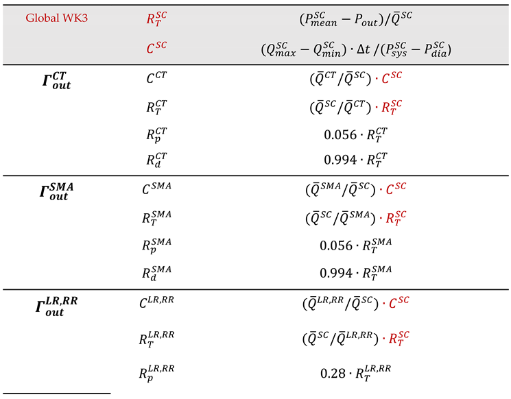 |
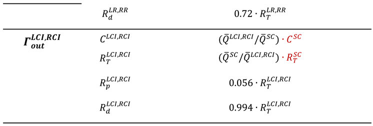 |
Appendix C
In literature, different vortex identification methods have been proposed. The most well-known vortex identification methods are Q-criterion, -criterion, -criterion and -criterion. All of those methods require different requirements to define a vortex. Q-criterion, -criterion, and -criterion are called as velocity gradient-based vortex identification criteria, while -criterion utilizes local pressure minimum to define a vortex.
Velocity gradient tensor can be partitioned into symmetric and antisymmetric parts
where and are the strain rate and angular rotation rate tensors, respectively. The trajectory of a fluid particle can be determined by solving the differential equation
with an initial condition Eigendecomposition of the above ordinary differential equation can be written as
where the columns of are eigenvectors and the diagonal of gives the eigenvalues . The general solution of the above equation is
where constants are determined from initial condition. According to the above equation, if all eigenvalues are real, then the point obtained is called as a node or a saddle. However, if one of the eigenvalues is real but the other two are complex conjugates, the point obtained becomes a focus, with closed or spiraling streamline trajectories, which is an indication of vortex.
To find the eigenvalues of diagonal, characteristic equations can be solved
which obtains
where P, Q and R are invariants of the velocity gradient tensor [241]. For an incompressible flow, is zero. The discriminant of the characteristic equation gives an idea whether the eigenvalues are real or complex, which can be written as
If , one eigenvalue is real, and the other two eigenvalues are complex conjugates, which indicates the swirling flow having a spiraling or closed streamline pattern, and this is called as -criterion. Q is the second invariant of the velocity gradient tensor, and for an incompressible flow, it is written as
Zhou et al. [287] also utilized the complex eigenvalue of the velocity gradient tensor to visualize vortices. For that purpose, they decompose velocity gradient tensor with the help of diagonalization by using eigenvalues and eigenvectors as following
where is the real eigenvalue with as corresponding real eigenvector , and are the conjugate pair of the complex eigenvalues with complex eigenvectors . The local streamlines can be expressed in a local coordinate as
where and are constants and can be determined from initial conditions. Along the axis of eigenvector , flow is either stretched or compressed, while flow is swirling on the plane of eigenvectors and . Hence, the imaginary parts, of complex eigenvalues might be evaluated as a vortex indicator and connected regions having non-zero can be specified as vortex structures. The complex eigenvector, , is known as strength of the swirling motion and it is called as the swirling strength of a vortex.
-criterion based on local pressure minimum across a vortex core. Jeong and Hussain [288] derived a transport equation for the strain rate tensor by taking gradient of the incompressible Navier Stokes equation, and obtain the symmetric part as follows
The term at the right-hand side is called as pressure Hessian matrix. According to -criterion, the vortex core is located to the local pressure minimum, except in the presence of unsteady and viscous effects. Therefore, by neglecting the rate of change of irrotational straining and viscous effects, pressure Hessian can be found as
Local pressure minimum can be obtained where the pressure Hessian has two positive eigenvalues, which requires term has two negative eigenvalues. In 3D flows, ordering the eigenvalues of this matrix should satisfy the two of them must be negative inside a vortex core
In 2D flows, should be two eigenvalues of the matrix. According to -criterion, must be negative, which identifies connected vortex zones.
References
- Lech, C.; Swaminathan, A. Abdominal Aortic Emergencies. Emerg Med Clin North Am 2017, 35 (4), 847–867. [CrossRef]
- Sakalihasan, N.; Michel, J. B.; Katsargyris, A.; Kuivaniemi, H.; Defraigne, J. O.; Nchimi, A.; Powell, J. T.; Yoshimura, K.; Hultgren, R. Abdominal Aortic Aneurysms. Nature Reviews Disease Primers. Nature Publishing Group December 1, 2018. [CrossRef]
- Dua, M. M.; Dalman, R. L. Hemodynamic Influences on Abdominal Aortic Aneurysm Disease: Application of Biomechanics to Aneurysm Pathophysiology. Vascular Pharmacology. July 2010, pp 11–21. [CrossRef]
- Darling, R. C.; Messina, C. R.; Brewster, D. C.; Ottinger, L. W. Autopsy Study of Unoperated Abdominal Aortic Aneurysms. The Case for Early Resection. Circulation 1977, 56 (3 Suppl), II161-4.
- Wang, X.; Ghayes, M. H.; Kotousov, A.; Zander, A. C.; Amabili, M.; Dawson, J. A.; Psaltis, P. J. Wang-2023-Biomechanics of Abdominal Aortic Aneurysm in the Framework Of. Int J Non Linear Mech 2023, 157. [CrossRef]
- Weintraub, N. L. Understanding Abdominal Aortic Aneurysm; 2009. [CrossRef]
- Saphirstein, R. J.; Morgan, K. G. The Contribution of Vascular Smooth Muscle to Aortic Stiffness across Length Scales. Microcirculation 2014, 21 (3), 201–207. [CrossRef]
- Soudah, E.; Ng, E. Y. K.; Loong, T. H.; Bordone, M.; Pua, U.; Narayanan, S. CFD Modelling of Abdominal Aortic Aneurysm on Hemodynamic Loads Using a Realistic Geometry with CT. Comput Math Methods Med 2013, 2013. [CrossRef]
- Boyd, A. J.; Kuhn, D. C. S.; Lozowy, R. J.; Kulbisky, G. P. Low Wall Shear Stress Predominates at Sites of Abdominal Aortic Aneurysm Rupture. J Vasc Surg 2016, 63 (6), 1613–1619. [CrossRef]
- Scotti, C. M.; Shkolnik, A. D.; Muluk, S. C.; Finol, E. A. Fluid-Structure Interaction in Abdominal Aortic Aneurysms: Effects of Asymmetry and Wall Thickness. Biomed Eng Online 2005, 4. [CrossRef]
- Wolters, B. J. B. M.; Rutten, M. C. M.; Schurink, G. W. H.; Kose, U.; De Hart, J.; Van De Vosse, F. N. A Patient-Specific Computational Model of Fluid-Structure Interaction in Abdominal Aortic Aneurysms. Med Eng Phys 2005, 27 (10), 871–883. [CrossRef]
- Papaharilaou, Y.; Ekaterinaris, J. A.; Manousaki, E.; Katsamouris, A. N. A Decoupled Fluid Structure Approach for Estimating Wall Stress in Abdominal Aortic Aneurysms. J Biomech 2007, 40 (2), 367–377. [CrossRef]
- Chandra, S.; Raut, S. S.; Jana, A.; Biederman, R. W.; Doyle, M.; Muluk, S. C.; Finol, E. A. Fluid-Structure Interaction Modeling of Abdominal Aortic Aneurysms: The Impact of Patient-Specific Inflow Conditions and Fluid/Solid Coupling. J Biomech Eng 2013, 135 (8). [CrossRef]
- Rengarajan, B.; Wu, W.; Wiedner, C.; Ko, D.; Muluk, S. C.; Eskandari, M. K.; Menon, P. G.; Finol, E. A. A Comparative Classification Analysis of Abdominal Aortic Aneurysms by Machine Learning Algorithms. Ann Biomed Eng 2020, 48 (4), 1419–1429. [CrossRef]
- Vorp, D. A. Biomechanics of Abdominal Aortic Aneurysm. J Biomech 2007, 40 (9), 1887–1902. [CrossRef]
- Blanco, P. J.; Watanabe, S. M.; Dari, E. A.; Passos, M. A. R. F.; Feijoo, R. A. Blood Flow Distribution in an Anatomically Detailed Arterial Network Model: Criteria and Algorithms. Biomech Model Mechanobiol 2014, 13, 1303–1330. [CrossRef]
- Xiao, N.; Alastruey, J.; Figueroa, C. A. A Systematic Comparison between 1-D and 3-D Hemodynamics in Compliant Arterial Models. Int J Numer Method Biomed Eng 2014, 30 (2), 204–231. [CrossRef]
- Zhou, S.; Xu, L.; Hao, L.; Xiao, H.; Yao, Y.; Qi, L.; Yao, Y. A Review on Low-Dimensional Physics-Based Models of Systemic Arteries: Application to Estimation of Central Aortic Pressure. BioMedical Engineering Online. BioMed Central Ltd. April 2, 2019. [CrossRef]
- Mirramezani, M.; Shadden, S. C. Distributed Lumped Parameter Modeling of Blood Flow in Compliant Vessels. J Biomech 2022, 140. [CrossRef]
- Zakerzadeh, R.; Cupac, T.; Dorfner, N.; Guy, A. Coupled Hemodynamics and Oxygen Diffusion in Abdominal Aortic Aneurysm: A Computational Sensitivity Study. Cardiovasc Eng Technol 2021, 12 (2), 166–182. [CrossRef]
- Ramazanli, B.; Sert, C.; Yavuz, M. M. Effect of Inlet Velocity Profile and Entrance Length on Abdominal Aortic Aneurysm Hemodynamics Simulations. Journal of Thermal Science and Technology 2023, 43 (2), 159–174. [CrossRef]
- Xiao, N.; Alastruey, J.; Figueroa, C. A. A Systematic Comparison between 1-D and 3-D Hemodynamics in Compliant Arterial Models. Int J Numer Method Biomed Eng 2014, 30 (2), 204–231. [CrossRef]
- Xiao, N.; Humphrey, J. D.; Figueroa, C. A. Multi-Scale Computational Model of Three-Dimensional Hemodynamics within a Deformable Full-Body Arterial Network. J Comput Phys 2013, 244, 22–40. [CrossRef]
- Liao, Z. J.; Qin, S.; Chen, R.; Cai, X. C. A Parallel Domain Decomposition Method for Large Eddy Simulation of Blood Flow in Human Artery with Resistive Boundary Condition. Comput Fluids 2022, 232. [CrossRef]
- Grinberg, L.; Karniadakis, G. E. Outflow Boundary Conditions for Arterial Networks with Multiple Outlets. Ann Biomed Eng 2008, 36 (9), 1496–1514. [CrossRef]
- Liu, H.; Liang, F.; Wong, J.; Fujiwara, T.; Ye, W.; Tsubota, K.; Sugawara, M. Multi-Scale Modeling of Hemodynamics in the Cardiovascular System. Acta Mechanica Sinica 2015, 31 (4), 446–464. [CrossRef]
- Sughimoto, K.; Takahara, Y.; Mogi, K.; Yamazaki, K.; Tsubota, K.; Liang, F.; Liu, H. Blood Flow Dynamic Improvement with Aneurysm Repair Detected by a Patient-Specific Model of Multiple Aortic Aneurysms. Heart Vessels 2014, 29 (3), 404–412. [CrossRef]
- Olufsen, M. S. Structured Tree Outflow Condition for Blood Flow in Larger Systemic Arteries. Am J Physiol 1999, 276 (1), 257–268. [CrossRef]
- Alastruey, J.; Khir, A. W.; Matthys, K. S.; Segers, P.; Sherwin, S. J.; Verdonck, P. R.; Parker, K. H.; Peiró, J. Pulse Wave Propagation in a Model Human Arterial Network: Assessment of 1-D Visco-Elastic Simulations against in Vitro Measurements. J Biomech 2011, 44 (12), 2250–2258. [CrossRef]
- Formaggia, L.; Lamponi, D.; Quarteroni, A. One-Dimensional Models for Blood Flow in Arteries. J Eng Math 2003, 47 (3), 251–276. [CrossRef]
- Olufsen, M. S.; Peskin, C. S.; Kim, W. Y.; Pedersen, E. M.; Nadim, A.; Larsen, J. Numerical Simulation and Experimental Validation of Blood Flow in Arteries with Structured-Tree Outflow Conditions. Ann Biomed Eng 2000, 28, 1281–1299.
- Xiao, N.; Humphrey, J. D.; Figueroa, C. A. Multi-Scale Computational Model of Three-Dimensional Hemodynamics within a Deformable Full-Body Arterial Network. J Comput Phys 2013, 244, 22–40. [CrossRef]
- Morris, P. D.; Narracott, A.; Von Tengg-Kobligk, H.; Alejandro, D.; Soto, S.; Hsiao, S.; Lungu, A.; Evans, P.; Bressloff, N. W.; Lawford, P. V; Hose, R.; Gunn, J. P. Computational Fluid Dynamics Modelling in Cardiovascular Medicine. Heart 2015, 102, 18–28. [CrossRef]
- Salman, H. E.; Ramazanli, B.; Yavuz, M. M.; Yalcin, H. C. Biomechanical Investigation of Disturbed Hemodynamics-Induced Tissue Degeneration in Abdominal Aortic Aneurysms Using Computational and Experimental Techniques. Front Bioeng Biotechnol 2019, 7. [CrossRef]
- Taylor, C. A.; Figueroa, C. A. Patient-Specific Modeling of Cardiovascular Mechanics. Annu Rev Biomed Eng 2009, 11, 109–134. [CrossRef]
- Les, A. S.; Yeung, J. J.; Schultz, G. M.; Herfkens, R. J.; Dalman, R. L.; Taylor, C. A. Supraceliac and Infrarenal Aortic Flow in Patients with Abdominal Aortic Aneurysms: Mean Flows, Waveforms, and Allometric Scaling Relationships. Cardiovasc Eng Technol 2010, 1 (1), 39–51. [CrossRef]
- Les, A. S.; Shadden, S. C.; Figueroa, C. A.; Park, J. M.; Tedesco, M. M.; Herfkens, R. J.; Dalman, R. L.; Taylor, C. A. Quantification of Hemodynamics in Abdominal Aortic Aneurysms during Rest and Exercise Using Magnetic Resonance Imaging and Computational Fluid Dynamics. Ann Biomed Eng 2010, 38 (4), 1288–1313. [CrossRef]
- Di Achille, P.; Tellides, G.; Figueroa, C. A.; Humphrey, J. D. A Haemodynamic Predictor of Intraluminal Thrombus Formation in Abdominal Aortic Aneurysms. Proceedings of the Royal Society A: Mathematical, Physical and Engineering Sciences 2014, 470 (2172). [CrossRef]
- Fonken, J. H. C.; Maas, E. J.; Nievergeld, A. H. M.; van Sambeek, M. R. H. M.; van de Vosse, F. N.; Lopata, R. G. P. Ultrasound-Based Fluid-Structure Interaction Modeling of Abdominal Aortic Aneurysms Incorporating Pre-Stress. Front Physiol 2021, 12. [CrossRef]
- Owen, B.; Lowe, C.; Ashton, N.; Mandal, P.; Rogers, S.; Wein, W.; McCollum, C.; Revell, A. Computational Hemodynamics of Abdominal Aortic Aneurysms: Three-Dimensional Ultrasound versus Computed Tomography. Proc Inst Mech Eng H 2016, 230 (3), 201–210. [CrossRef]
- Qiu, Y.; Yuan, D.; Wang, Y.; Wen, J.; Zheng, T. Hemodynamic Investigation of a Patient-Specific Abdominal Aortic Aneurysm with Iliac Artery Tortuosity. Comput Methods Biomech Biomed Engin 2018, 21 (16), 824–833. [CrossRef]
- Qiu, Y.; Wang, Y.; Fan, Y.; Peng, L.; Liu, R.; Zhao, J.; Yuan, D.; Zheng, T. Role of Intraluminal Thrombus in Abdominal Aortic Aneurysm Ruptures: A Hemodynamic Point of View. Med Phys 2019, 46 (9), 4263–4275. [CrossRef]
- Teng, B.; Zhou, Z.; Zhao, Y.; Wang, Z. Combined Curvature and Wall Shear Stress Analysis of Abdominal Aortic Aneurysm: An Analysis of Rupture Risk Factors. Cardiovasc Intervent Radiol 2022, 45 (6), 752–760. [CrossRef]
- Mei, Y.; Xu, H.; Ma, W.; Li, Z.; Yang, R.; Yuan, H.; Peng, Y.; Wu, M.; Chen, Z.; Guo, W.; Gao, T.; Xiong, J.; Chen, D. Retrograde Branched Extension Limb Assembling Stent of Pararenal Abdominal Aortic Aneurysm: A Longitudinal Hemodynamic Analysis for Stent Graft Migration. Int J Numer Method Biomed Eng 2020, 36 (11). [CrossRef]
- Zhou, J.; Li, J.; Qin, S.; Guo, W.; Chen, R. Hemodynamic Simulation of Aneurysmal Aorta Using a Parallel Algorithm and a Flow-Rate Based Resistance Splitting Method. Computers and Electrical Engineering 2022, 104. [CrossRef]
- Dzieciuchowicz, Ł.; Krzyżański, R.; Nowak, A. Use of Intravascular Ultrasound in Endovascular Repair of Abdominal Aortic Aneurysm. Postepy w Kardiologii Interwencyjnej. Termedia Publishing House Ltd. 2020, pp 202–205. [CrossRef]
- Van Rooij, W. J.; Sprengers, M. E.; De Gast, A. N.; Peluso, J. P. P.; Sluzewski, M. 3D Rotational Angiography: The New Gold Standard in the Detection of Additional Intracranial Aneurysms. In American Journal of Neuroradiology; 2008; Vol. 29, pp 976–979. [CrossRef]
- Mai, D. V. C.; Drami, I.; Pring, E. T.; Gould, L. E.; Lung, P.; Popuri, K.; Chow, V.; Beg, M. F.; Athanasiou, T.; Jenkins, J. T. A Systematic Review of Automated Segmentation of 3D Computed-Tomography Scans for Volumetric Body Composition Analysis. Journal of Cachexia, Sarcopenia and Muscle. John Wiley and Sons Inc October 1, 2023, pp 1973–1986. [CrossRef]
- Badrinarayanan, V.; Kendall, A.; Cipolla, R. SegNet: A Deep Convolutional Encoder-Decoder Architecture for Image Segmentation. IEEE Trans Pattern Anal Mach Intell 2017, 39 (12), 2481–2495. [CrossRef]
- Bhalerao, M.; Thakur, S. Brain Tumor Segmentation Based on 3D Residual U-Net. In Lecture Notes in Computer Science (including subseries Lecture Notes in Artificial Intelligence and Lecture Notes in Bioinformatics); Springer, 2020; Vol. 11993 LNCS, pp 218–225. [CrossRef]
- Mu, N.; Lyu, Z.; Rezaeitaleshmahalleh, M.; Tang, J.; Jiang, J. An Attention Residual U-Net with Differential Preprocessing and Geometric Postprocessing: Learning How to Segment Vasculature Including Intracranial Aneurysms. Med Image Anal 2023, 84, 102697. [CrossRef]
- Mu, N.; Lyu, Z.; Rezaeitaleshmahalleh, M.; Zhang, X.; Rasmussen, T.; McBane, R.; Jiang, J. Automatic Segmentation of Abdominal Aortic Aneurysms from CT Angiography Using a Context-Aware Cascaded U-Net. Comput Biol Med 2023, 158, 106569. [CrossRef]
- Chung, T. K.; Liang, N. L.; Vorp, D. A. Artificial Intelligence Framework to Predict Wall Stress in Abdominal Aortic Aneurysm. Applications in Engineering Science 2022, 10. [CrossRef]
- Lan, I. S.; Liu, J.; Yang, W.; Marsden, A. L. Numerical Investigation of Abdominal Aortic Aneurysm Hemodynamics Using the Reduced Unified Continuum Formulation for Vascular Fluid-Structure Interaction. Forces in Mechanics 2022, 7. [CrossRef]
- Peng, C.; He, W.; Huang, X.; Ma, J.; Yuan, T.; Shi, Y.; Wang, S. The Study on the Impact of AAA Wall Motion on the Hemodynamics Based on 4D CT Image Data. Front Bioeng Biotechnol 2023, 11. [CrossRef]
- Arslan, A. C.; Salman, H. E. Effect of Intraluminal Thrombus Burden on the Risk of Abdominal Aortic Aneurysm Rupture. J Cardiovasc Dev Dis 2023, 10 (6). [CrossRef]
- Brambila-Solórzano, A.; Méndez-Lavielle, F.; Naude, J. L.; Martínez-Sánchez, G. J.; García-Rebolledo, A.; Hernández, B.; Escobar-del Pozo, C. Influence of Blood Rheology and Turbulence Models in the Numerical Simulation of Aneurysms. Bioengineering 2023, 10 (10). [CrossRef]
- Drewe, C. J.; Parker, L. P.; Kelsey, L. J.; Norman, P. E.; Powell, J. T.; Doyle, B. J. Haemodynamics and Stresses in Abdominal Aortic Aneurysms: A Fluid-Structure Interaction Study into the Effect of Proximal Neck and Iliac Bifurcation Angle. J Biomech 2017, 60, 150–156. [CrossRef]
- Wang-2023-Biomechanics of Abdominal Aortic Aneurysm in the Framework Of.
- Jayendiran, R.; Nour, B.; Ruimi, A. Computational Analysis of Nitinol Stent-Graft for Endovascular Aortic Repair (EVAR) of Abdominal Aortic Aneurysm (AAA): Crimping, Sealing and Fluid-Structure Interaction (FSI). Int J Cardiol 2020, 304, 164–171. [CrossRef]
- Kaewchoothong, N.; Algabri, Y. A.; Assawalertsakul, T.; Nuntadusit, C.; Chatpun, S. Computational Study of Abdominal Aortic Aneurysms with Severely Angulated Neck Based on Transient Hemodynamics Using an Idealized Model. Applied Sciences (Switzerland) 2022, 12 (4). [CrossRef]
- Moradicheghamahi, J. The Role of Wall Mechanics in the Hemodynamics of a Realistic Abdominal Aortic Aneurysm: A Fluid-Structure Interaction Study. Journal of Engineering 2024, 2024, 1–19. [CrossRef]
- Piccinelli, M.; Vergara, C.; Antiga, L.; Forzenigo, L.; Biondetti, P.; Domanin, M. Impact of Hemodynamics on Lumen Boundary Displacements in Abdominal Aortic Aneurysms by Means of Dynamic Computed Tomography and Computational Fluid Dynamics. Biomech Model Mechanobiol 2013, 12 (6), 1263–1276. [CrossRef]
- Suh, G. Y.; Les, A. S.; Tenforde, A. S.; Shadden, S. C.; Spilker, R. L.; Yeung, J. J.; Cheng, C. P.; Herfkens, R. J.; Dalman, R. L.; Taylor, C. A. Quantification of Particle Residence Time in Abdominal Aortic Aneurysms Using Magnetic Resonance Imaging and Computational Fluid Dynamics. Ann Biomed Eng 2011, 39 (2), 864–883. [CrossRef]
- Suh, G. Y.; Les, A. S.; Tenforde, A. S.; Shadden, S. C.; Spilker, R. L.; Yeung, J. J.; Cheng, C. P.; Herfkens, R. J.; Dalman, R. L.; Taylor, C. A. Hemodynamic Changes Quantified in Abdominal Aortic Aneurysms with Increasing Exercise Intensity Using MR Exercise Imaging and Image-Based Computational Fluid Dynamics. Ann Biomed Eng 2011, 39 (8), 2186–2202. [CrossRef]
- Bologna, E.; Dinoto, E.; Di Simone, F.; Pecoraro, F.; Ragusa, S.; Siciliano, K.; Zingales, M. Computational Fluid Dynamics (CFD) and Finite Element Analysis (FEM) of a Customized Stent-Graft for Endovascular (EVAR) Treatment of Abdominal Aortic Aneurism (AAA). Applied Sciences (Switzerland) 2023, 13 (9). [CrossRef]
- Al-Jumaily, A. M.; Embong, A. H. Bin; AL-Rawi, M.; Mahadevan, G.; Sugita, S. Aneurysm Rupture Prediction Based on Strain Energy-CFD Modelling. Bioengineering 2023, 10 (10). [CrossRef]
- Scotti, C. M.; Finol, E. A. Compliant Biomechanics of Abdominal Aortic Aneurysms: A Fluid-Structure Interaction Study. Comput Struct 2007, 85 (11–14), 1097–1113. [CrossRef]
- Scotti, C. M.; Jimenez, J.; Muluk, S. C.; Finol, E. A. Wall Stress and Flow Dynamics in Abdominal Aortic Aneurysms: Finite Element Analysis vs. Fluid-Structure Interaction. Comput Methods Biomech Biomed Engin 2008, 11 (3), 301–322. [CrossRef]
- Torii, R.; Oshima, M.; Kobayashi, T.; Takagi, K.; Tezduyar, T. E. Numerical Investigation of the Effect of Hypertensive Blood Pressure on Cerebral Aneurysm - Dependence of the Effect on the Aneurysm Shape. Int J Numer Methods Fluids 2007, 54 (6–8), 995–1009. [CrossRef]
- Torii, R.; Oshima, M.; Kobayashi, T.; Takagi, K.; Tezduyar, T. E. Computer Modeling of Cardiovascular Fluid-Structure Interactions with the Deforming-Spatial-Domain/Stabilized Space-Time Formulation. Comput Methods Appl Mech Eng 2006, 195 (13–16), 1885–1895. [CrossRef]
- Arzani, A.; Shadden, S. C. Characterizations and Correlations of Wall Shear Stress in Aneurysmal Flow. J Biomech Eng 2016, 138 (1). [CrossRef]
- Bessonov, N.; Sequeira, A.; Simakov, S.; Vassilevskii, Y.; Volpert, V. Methods of Blood Flow Modelling. Math Model Nat Phenom 2016, 11 (1), 1–25. [CrossRef]
- Ebrahimi, S.; Mirafzal, I.; Rahbary, A.; Shamloo, A.; Naseri, T. Optimization of Nano-Microparticle Size and Shape on Wall-Interaction: A Human Case Study on an Abdominal Aortic Aneurysm. Engineering Applications of Computational Fluid Mechanics 2023, 17 (1). [CrossRef]
- Arzani, A. Accounting for Residence-Time in Blood Rheology Models: Do We Really Need Non-Newtonian Blood Flow Modelling in Large Arteries? J R Soc Interface 2018, 15 (146). [CrossRef]
- Biasetti, J.; Hussain, F.; Christian Gasser, T. Blood Flow and Coherent Vortices in the Normal and Aneurysmatic Aortas: A Fluid Dynamical Approach to Intraluminal Thrombus Formation. J R Soc Interface 2011, 8 (63), 1449–1461. [CrossRef]
- Bilgi, C.; Atalik, K. Numerical Investigation of the Effects Ofblood Rheology and Wall Elasticity in Abdominal Aortic Aneurysm under Pulsatile Flow Conditions. Biorheology 2019, 56 (1), 51–71. [CrossRef]
- Marrero, V. L.; Tichy, J. A.; Sahni, O.; Jansen, K. E. Numerical Study of Purely Viscous Non-Newtonian Flow in an Abdominal Aortic Aneurysm. J Biomech Eng 2014, 136 (10). [CrossRef]
- Childress, E. M.; Kleinstreuer, C. Impact of Fluid-Structure Interaction on Direct Tumor-Targeting in a Representative Hepatic Artery System. Ann Biomed Eng 2014, 42 (3), 461–474. [CrossRef]
- Razavi, A.; Shirani, E.; Sadeghi, M. R. Numerical Simulation of Blood Pulsatile Flow in a Stenosed Carotid Artery Using Different Rheological Models. J Biomech 2011, 44 (11), 2021–2030. [CrossRef]
- Morbiducci, U.; Ponzini, R.; Gallo, D.; Bignardi, C.; Rizzo, G. Inflow Boundary Conditions for Image-Based Computational Hemodynamics: Impact of Idealized versus Measured Velocity Profiles in the Human Aorta. J Biomech 2013, 46 (1), 102–109. [CrossRef]
- Mendieta, J. B.; Fontanarosa, D.; Wang, J.; Paritala, P. K.; McGahan, T.; Lloyd, T.; Li, Z. The Importance of Blood Rheology in Patient-Specific Computational Fluid Dynamics Simulation of Stenotic Carotid Arteries. Biomech Model Mechanobiol 2020, 19 (5), 1477–1490. [CrossRef]
- Karimi, S.; Dabagh, M.; Vasava, P.; Dadvar, M.; Dabir, B.; Jalali, P. Effect of Rheological Models on the Hemodynamics within Human Aorta: CFD Study on CT Image-Based Geometry. J Nonnewton Fluid Mech 2014, 207, 42–52. [CrossRef]
- Faraji, A.; Sahebi, M.; SalavatiDezfouli, S. Numerical Investigation of Different Viscosity Models on Pulsatile Blood Flow of Thoracic Aortic Aneurysm (TAA) in a Patient-Specific Model. Comput Methods Biomech Biomed Engin 2023, 26 (8), 986–998. [CrossRef]
- Skiadopoulos, A.; Neofytou, P.; Housiadas, C. Comparison of Blood Rheological Models in Patient Specific Cardiovascular System Simulations. J Hydrodynam B 2017, 29 (2), 293–304. [CrossRef]
- Cho, Y. I.; Kensey, K. R. Effects of the Non-Newtonian Viscosity of Blood on Flows in a Diseased Arterial Vessel. Part 1: Steady Flows. Biorheology 1991, 28 (3–4), 241–262. [CrossRef]
- Leuprecht, A.; Perktold, K. Computer Simulation of Non-Newtonian Effects on Blood Flow in Large Arteries. Comput Methods Biomech Biomed Engin 2001, 4 (2), 149–163. [CrossRef]
- Quemada, D. Rheology of Concentrated Disperse Systems III. General Features of the Proposed Non-Newtonian Model. Comparison with Experimental Data. Rheol Acta 1978, 17 (6), 643–653. [CrossRef]
- Bilgi, C.; Atalık, K. Effects of Blood Viscoelasticity on Pulsatile Hemodynamics in Arterial Aneurysms. J Nonnewton Fluid Mech 2020, 279. [CrossRef]
- Bodnár, T.; Sequeira, A.; Prosi, M. On the Shear-Thinning and Viscoelastic Effects of Blood Flow under Various Flow Rates. Appl Math Comput 2011, 217 (11), 5055–5067. [CrossRef]
- Guranov, I.; Ćoćić, A.; Lečić, M. Numerical Studies of Viscoelastic Flow Using the Software OpenFOAM. PAMM 2013, 13 (1), 591–592. [CrossRef]
- Habla, F.; Tan, M. W.; Haßlberger, J.; Hinrichsen, O. Numerical Simulation of the Viscoelastic Flow in a Three-Dimensional Lid-Driven Cavity Using the Log-Conformation Reformulation in OpenFOAM®. J Nonnewton Fluid Mech 2014, 212, 47–62. [CrossRef]
- Elhanafy, A.; Guaily, A.; Elsaid, A. Numerical Simulation of Oldroyd-B Fluid with Application to Hemodynamics. Advances in Mechanical Engineering 2019, 11 (5), 1687814019852844. [CrossRef]
- Wang, X.; Carpenter, H. J.; Ghayesh, M. H.; Kotousov, A.; Zander, A. C.; Amabili, M.; Psaltis, P. J. A Review on the Biomechanical Behaviour of the Aorta. Journal of the Mechanical Behavior of Biomedical Materials. Elsevier Ltd August 1, 2023. [CrossRef]
- Holzapfel, G. A.; Ogden, R. W. Constitutive Modelling of Arteries. In Proceedings of the Royal Society A: Mathematical, Physical and Engineering Sciences; Royal Society, 2010; Vol. 466, pp 1551–1597. [CrossRef]
- Humphrey, J. D.; Holzapfel, G. A. Mechanics, Mechanobiology, and Modeling of Human Abdominal Aorta and Aneurysms. Journal of Biomechanics. March 15, 2012, pp 805–814. [CrossRef]
- Tong, J.; Holzapfel, G. A. Structure, Mechanics, and Histology of Intraluminal Thrombi in Abdominal Aortic Aneurysms. Ann Biomed Eng 2015, 43 (7), 1488–1501. [CrossRef]
- Holzapfel, G. A.; Gasser, T. C.; Ogden, R. W. A New Constitutive Framework for Arterial Wall Mechanics and a Comparative Study of Material Models. Journal of elasticity and the physical science of solids 2000, 61 (1), 1–48. https://hal.science/hal-01297725.
- Raghavan, M. L.; Vorp, D. A. Toward a Biomechanical Tool to Evaluate Rupture Potential of Abdominal Aortic Aneurysm: Identi"cation of a "nite Strain Constitutive Model and Evaluation of Its Applicability. J Biomech 2000, 33, 475–482.
- Martino, E. S. Di; Guadagni, G.; Fumero, A.; Ballerini, G.; Spirito, R.; Biglioli, P.; Redaelli, A. Fluid-Structure Interaction within Realistic Three-Dimensional Models of the Aneurysmatic Aorta as a Guidance to Assess the Risk of Rupture of the Aneurysm; 2001; Vol. 23. www.elsevier.com/locate/medengphy.
- Salman, H. E.; Yalcin, H. C. Computational Investigation of the Effect of Wall Thickness on Rupture Risk in Abdominal Aortic Aneurysms. Journal of Applied Fluid Mechanics 2021, 14 (2), 499–513. [CrossRef]
- Javadzadegan, A.; Fakhim, B.; Behnia, M.; Behnia, M. Fluid-Structure Interaction Investigation of Spiral Flow in a Model of Abdominal Aortic Aneurysm. European Journal of Mechanics, B/Fluids 2014, 46, 109–117. [CrossRef]
- Khanafer, K.; Berguer, R. Fluid-Structure Interaction Analysis of Turbulent Pulsatile Flow within a Layered Aortic Wall as Related to Aortic Dissection. J Biomech 2009, 42 (16), 2642–2648. [CrossRef]
- Gao, F.; Ueda, H.; Gang, L.; Okada, H. Fluid Structure Interaction Simulation in Three-Layered Aortic Aneurysm Model under Pulsatile Flow: Comparison of Wrapping and Stenting. J Biomech 2013, 46 (7), 1335–1342. [CrossRef]
- Simsek, F. G.; Kwon, Y. W. Investigation of Material Modeling in Fluid–Structure Interaction Analysis of an Idealized Three-Layered Abdominal Aorta: Aneurysm Initiation and Fully Developed Aneurysms. J Biol Phys 2015, 41 (2), 173–201. [CrossRef]
- Fan, X.; Zhang, A.; Zheng, Q.; Li, P.; Wang, Y.; He, L.; Xue, Y.; Chen, W.; Wu, X.; Zhao, Y.; Wang, Y. The Biomechanical Effects of Different Membrane Layer Structures and Material Constitutive Modeling on Patient-Specific Cerebral Aneurysms. Front Bioeng Biotechnol 2023, 11. [CrossRef]
- Gasser, T. C.; Miller, C.; Polzer, S.; Roy, J. A Quarter of a Century Biomechanical Rupture Risk Assessment of Abdominal Aortic Aneurysms. Achievements, Clinical Relevance, and Ongoing Developments. Int J Numer Method Biomed Eng 2023, 39 (4). [CrossRef]
- Bluestein, D.; Dumont, K.; De Beule, M.; Ricotta, J.; Impellizzeri, P.; Verhegghe, B.; Verdonck, P. Intraluminal Thrombus and Risk of Rupture in Patient Specific Abdominal Aortic Aneurysm - FSI Modelling. Comput Methods Biomech Biomed Engin 2009, 12 (1), 73–81. [CrossRef]
- Lin, S.; Han, X.; Bi, Y.; Ju, S.; Gu, L. Fluid-Structure Interaction in Abdominal Aortic Aneurysm: Effect of Modeling Techniques. Biomed Res Int 2017, 2017. [CrossRef]
- Stevens, R. R. F.; Grytsan, A.; Biasetti, J.; Roy, J.; Liljeqvist, M. L.; Christian Gasser, T. Biomechanical Changes during Abdominal Aortic Aneurysm Growth. PLoS One 2017, 12 (11). [CrossRef]
- Balzani, D.; Heinlein, A.; Klawonn, A.; Rheinbach, O.; Schröder, J. Comparison of Arterial Wall Models in Fluid–Structure Interaction Simulations. Comput Mech 2023, 72 (5), 949–965. [CrossRef]
- Józsa, T. I.; Paál, G. Boundary Conditions for Flow Simulations of Abdominal Aortic Aneurysms. Int J Heat Fluid Flow 2014, 50, 342–351. [CrossRef]
- Keramati, H.; Birgersson, E.; Ho, J. P.; Kim, S.; Chua, K. J.; Leo, H. L. The Effect of the Entry and Re-Entry Size in the Aortic Dissection: A Two-Way Fluid–Structure Interaction Simulation. Biomech Model Mechanobiol 2020, 19 (6), 2643–2656. [CrossRef]
- Vande Geest, J. P.; Wang, D. H. J.; Wisniewski, S. R.; Makaroun, M. S.; Vorp, D. A. Towards A Noninvasive Method for Determination of Patient-Specific Wall Strength Distribution in Abdominal Aortic Aneurysms. Ann Biomed Eng 2006, 34 (7), 1098–1106. [CrossRef]
- Vande Geest, J. P.; Sacks, M. S.; Vorp, D. A. A Planar Biaxial Constitutive Relation for the Luminal Layer of Intra-Luminal Thrombus in Abdominal Aortic Aneurysms. J Biomech 2006, 39 (13), 2347–2354. [CrossRef]
- Raut, S. S.; Jana, A.; De Oliveira, V.; Muluk, S. C.; Finol, E. A. The Effect of Uncertainty in Vascular Wall Material Properties on Abdominal Aortic Aneurysm Wall Mechanics. In Computational Biomechanics for Medicine: Fundamental Science and Patient-Specific Applications; Springer New York, 2014; Vol. 9781493907458, pp 69–86. [CrossRef]
- Polzer, S.; Gasser, T. C. Biomechanical Rupture Risk Assessment of Abdominal Aortic Aneurysms Based on a Novel Probabilistic Rupture Risk Index. J R Soc Interface 2015, 12 (113). [CrossRef]
- Federico, S.; Grillo, A.; Giaquinta, G.; Herzog, W. Convex Fung-Type Potentials for Biological Tissues. Meccanica 2008, 43 (3), 279–288. [CrossRef]
- Gasser, T. C.; Ogden, R. W.; Holzapfel, G. A. Hyperelastic Modelling of Arterial Layers with Distributed Collagen Fibre Orientations. J R Soc Interface 2006, 3 (6), 15–35. [CrossRef]
- Chuong, C. J.; Fung, Y. C. Three-Dimensional Stress Distribution in Arteries. J Biomech Eng 1983, 105 (3), 268–274. [CrossRef]
- Holzapfel, G. A.; Gasser, T. C. A Viscoelastic Model for Fiber-Reinforced Composites at Finite Strains: Continuum Basis, Computational Aspects and Applications. Comput Methods Appl Mech Eng 2001, 190 (34), 4379–4403. [CrossRef]
- Choi, H. S.; Vito, R. P. Two-Dimensional Stress-Strain Relationship for Canine Pericardium. J Biomech Eng 1990, 112 (2), 153–159. [CrossRef]
- Di Martino, E. S.; Vorp, D. A. Effect of Variation in Intraluminal Thrombus Constitutive Properties on Abdominal Aortic Aneurysm Wall Stress. Ann Biomed Eng 2003, 31 (7), 804–809. [CrossRef]
- Xenos, M.; Labropoulos, N.; Rambhia, S.; Alemu, Y.; Einav, S.; Tassiopoulos, A.; Sakalihasan, N.; Bluestein, D. Progression of Abdominal Aortic Aneurysm Towards Rupture: Refining Clinical Risk Assessment Using a Fully Coupled Fluid–Structure Interaction Method. Ann Biomed Eng 2015, 43 (1), 139–153. [CrossRef]
- De Borst, R.; Nithiarasu, P.; Tezduyar, T. E.; Yagawa, G.; Zohdi, T. COMPUTATIONAL FLUID-STRUCTURE INTERACTION WILEY SERIES IN COMPUTATIONAL MECHANICS Series Advisors; Wiley Series in Computational echanicsa, 2013.
- Reymond, P.; Crosetto, P.; Deparis, S.; Quarteroni, A.; Stergiopulos, N. Physiological Simulation of Blood Flow in the Aorta: Comparison of Hemodynamic Indices as Predicted by 3-D FSI, 3-D Rigid Wall and 1-D Models. Med Eng Phys 2013, 35 (6), 784–791. [CrossRef]
- Crosetto, P.; Reymond, P.; Deparis, S.; Kontaxakis, D.; Stergiopulos, N.; Quarteroni, A. Fluid-Structure Interaction Simulation of Aortic Blood Flow. Comput Fluids 2011, 43 (1), 46–57. [CrossRef]
- Takizawa, K.; Christopher, J.; Tezduyar, T. E.; Sathe, S. Space-Time Finite Element Computation of Arterial Fluid-Structure Interactions with Patient-Specific Data. Int J Numer Method Biomed Eng 2010, 26 (1), 101–116. [CrossRef]
- Donea, J.; Giuliani, S.; Halleux, J. P. An Arbitrary Lagrangian-Eulerian Finite Element Method for Transient Dynamic Fluid-Structure Interactions. Comput Methods Appl Mech Eng 1982, 33, 689–723.
- Pirola, S.; Cheng, Z.; Jarral, O. A.; O’Regan, D. P.; Pepper, J. R.; Athanasiou, T.; Xu, X. Y. On the Choice of Outlet Boundary Conditions for Patient-Specific Analysis of Aortic Flow Using Computational Fluid Dynamics. J Biomech 2017, 60, 15–21. [CrossRef]
- Mariotti, A.; Boccadifuoco, A.; Celi, S.; Salvetti, M. V. Hemodynamics and Stresses in Numerical Simulations of the Thoracic Aorta: Stochastic Sensitivity Analysis to Inlet Flow-Rate Waveform. Comput Fluids 2021, 230. [CrossRef]
- Kim, H. J.; Vignon-Clementel, I. E.; Figueroa, C. A.; Ladisa, J. F.; Jansen, K. E.; Feinstein, J. A.; Taylor, C. A. On Coupling a Lumped Parameter Heart Model and a Three-Dimensional Finite Element Aorta Model. Ann Biomed Eng 2009, 37 (11), 2153–2169. [CrossRef]
- Bonfanti, M.; Franzetti, G.; Maritati, G.; Homer-Vanniasinkam, S.; Balabani, S.; Díaz-Zuccarini, V. Patient-Specific Haemodynamic Simulations of Complex Aortic Dissections Informed by Commonly Available Clinical Datasets. Med Eng Phys 2019, 71, 45–55. [CrossRef]
- Formaggia, L.; Lamponi, D.; Tuveri, M.; Veneziani, A. Numerical Modeling of 1D Arterial Networks Coupled with a Lumped Parameters Description of the Heart. Comput Methods Biomech Biomed Engin 2006, 9 (5), 273–288. [CrossRef]
- Alastruey, J.; Xiao, N.; Fok, H.; Schaeffter, T.; Figueroa, C. A. On the Impact of Modelling Assumptions in Multi-Scale, Subject-Specific Models of Aortic Haemodynamics. J R Soc Interface 2016, 13 (119). [CrossRef]
- van ’t Veer, M.; Buth, J.; Merkx, M.; Tonino, P.; van den Bosch, H.; Pijls, N.; van de Vosse, F. Biomechanical Properties of Abdominal Aortic Aneurysms Assessed by Simultaneously Measured Pressure and Volume Changes in Humans. J Vasc Surg 2008, 48 (6), 1401–1407. [CrossRef]
- Youssefi, P.; Gomez, A.; Arthurs, C.; Sharma, R.; Jahangiri, M.; Figueroa, C. A. Impact of Patient-Specific Inflow Velocity Profile on Hemodynamics of the Thoracic Aorta. J Biomech Eng 2018, 140 (1). [CrossRef]
- Cheng, Z.; Kidher, E.; Jarral, O. A.; O’Regan, D. P.; Wood, N. B.; Athanasiou, T.; Xu, X. Y. Assessment of Hemodynamic Conditions in the Aorta Following Root Replacement with Composite Valve-Conduit Graft. Ann Biomed Eng 2016, 44 (5), 1392–1404. [CrossRef]
- Pirola, S.; Guo, B.; Menichini, C.; Saitta, S.; Fu, W.; Dong, Z.; Xu, X. Y. 4-D Flow Mri-Based Computational Analysis of Blood Flow in Patient-Specific Aortic Dissection. IEEE Trans Biomed Eng 2019, 66 (12), 3411–3419. [CrossRef]
- Markl, M.; Schnell, S.; Wu, C.; Bollache, E.; Jarvis, K.; Barker, A. J.; Robinson, J. D.; Rigsby, C. K. Advanced Flow MRI: Emerging Techniques and Applications. Clin Radiol 2016, 71 (8), 779–795. [CrossRef]
- Lodi Rizzini, M.; Gallo, D.; De Nisco, G.; D’Ascenzo, F.; Chiastra, C.; Bocchino, P. P.; Piroli, F.; De Ferrari, G. M.; Morbiducci, U. Does the Inflow Velocity Profile Influence Physiologically Relevant Flow Patterns in Computational Hemodynamic Models of Left Anterior Descending Coronary Artery? Med Eng Phys 2020, 82, 58–69. [CrossRef]
- Armour, C. H.; Guo, B.; Pirola, S.; Saitta, S.; Liu, Y.; Dong, Z.; Xu, X. Y. The Influence of Inlet Velocity Profile on Predicted Flow in Type B Aortic Dissection. Biomech Model Mechanobiol 2021, 20 (2), 481–490. [CrossRef]
- Chen, X.; Zhuang, J.; Wu, Y. The Effect of Womersley Number and Particle Radius on the Accumulation of Lipoproteins in the Human Aorta. Comput Methods Biomech Biomed Engin 2020, 23 (10), 571–584. [CrossRef]
- Bit, A.; Alblawi, A.; Chattopadhyay, H.; Quais, Q. A.; Benim, A. C.; Rahimi-Gorji, M.; Do, H. T. Three Dimensional Numerical Analysis of Hemodynamic of Stenosed Artery Considering Realistic Outlet Boundary Conditions. Comput Methods Programs Biomed 2020, 185, 105163. [CrossRef]
- Colciago, C. M.; Deparis, S.; Domanin, M.; Riccobene, C.; Schenone, E.; Quarteroni, A. Analysis of Morphological and Haemodynamical Indexes in Abdominal Aortic Aneurysms as Preliminary Indicators of Intraluminal Thrombus Deposition. Biomech Model Mechanobiol 2020, 19, 1035–1053. [CrossRef]
- Arzani, A.; Suh, G. Y.; Dalman, R. L.; Shadden, S. C. A Longitudinal Comparison of Hemodynamics and Intraluminal Thrombus Deposition in Abdominal Aortic Aneurysms. Am J Physiol Heart Circ Physiol 2014, 307 (12), H1786–H1795. [CrossRef]
- Choudhury, S.; Anupindi, K.; Patnaik, B. S. V. Influence of Wall Shear Stress and Geometry on the Lumen Surface Concentration of Low Density Lipoprotein in a Model Abdominal Aortic Aneurysm. Physics of Fluids 2019, 31 (1). [CrossRef]
- Hardman, D.; Semple, S. I.; Richards, J. M. J.; Hoskins, P. R. Comparison of Patient-Specific Inlet Boundary Conditions in the Numerical Modelling of Blood Flow in Abdominal Aortic Aneurysm Disease. Int J Numer Method Biomed Eng 2013, 29 (2), 165–178. [CrossRef]
- Lozowy, R. J.; Kuhn, D. C. S.; Ducas, A. A.; Boyd, A. J. The Relationship Between Pulsatile Flow Impingement and Intraluminal Thrombus Deposition in Abdominal Aortic Aneurysms. Cardiovasc Eng Technol 2017, 8 (1), 57–69. [CrossRef]
- Wei, Z. A.; Huddleston, C.; Trusty, P. M.; Singh-Gryzbon, S.; Fogel, M. A.; Veneziani, A.; Yoganathan, A. P. Analysis of Inlet Velocity Profiles in Numerical Assessment of Fontan Hemodynamics. Ann Biomed Eng 2019, 47 (11), 2258–2270. [CrossRef]
- Tzirakis, K.; Kamarianakis, Y.; Kontopodis, N.; Ioannou, C. V. The Effect of Blood Rheology and Inlet Boundary Conditions on Realistic Abdominal Aortic Aneurysms under Pulsatile Flow Conditions. Bioengineering 2023, 10 (2). [CrossRef]
- Womersley, J. R. Method for the Calculation of Velocity, Rate of Flow and Viscous Drag in Arteries When the Pressure Gradient Is Known. J Physiol 1955, 127 (3), 553–563. [CrossRef]
- Campbell, I. C.; Ries, J.; Dhawan, S. S.; Quyyumi, A. A.; Taylor, W. R.; Oshinski, J. N. Effect of Inlet Velocity Profiles on Patient-Specific Computational Fluid Dynamics Simulations of the Carotid Bifurcation. J Biomech Eng 2012, 134 (5). [CrossRef]
- Impiombato, A. N.; La Civita, G.; Orlandi, F.; Franceschini Zinani, F. S.; Oliveira Rocha, L. A.; Biserni, C. A Simple Transient Poiseuille-Based Approach to Mimic the Womersley Function and to Model Pulsatile Blood Flow. Dynamics 2021, 1 (1), 9–17. [CrossRef]
- Madhavan, S.; Kemmerling, E. M. C. The Effect of Inlet and Outlet Boundary Conditions in Image-Based CFD Modeling of Aortic Flow. Biomed Eng Online 2018, 17 (1). [CrossRef]
- Li, Z.; Mao, W. Li-2023-A Fast Approach to Estimating Windkessel Model Parameters For. Comput Fluids 2023, 259. [CrossRef]
- Javadzadegan, A.; Simmons, A.; Behnia, M.; Barber, T. Computational Modelling of Abdominal Aortic Aneurysms: Effect of Suprarenal vs Infrarenal Positions. European Journal of Mechanics, B/Fluids 2017, 61, 112–124. [CrossRef]
- Von Spiczak, J.; Crelier, G.; Giese, D.; Kozerke, S.; Maintz, D.; Bunck, A. C. Quantitative Analysis of Vortical Blood Flow in the Thoracic Aorta Using 4D Phase Contrast MRI. PLoS One 2015, 10 (9). [CrossRef]
- Stonebridge, P.; Thompson, A.; Dick, J.; Hunter, G.; Chudek, J. A.; Houston, J.; Belch, J. Non Spiral and Spiral (Helical) Flow Patterns in Stenoses. In Vitro Observations Using Spin and Gradient Echo Magnetic Resonance Imaging (MRI) and Computational Fluid Dynamic Modeling. Int Angiol 2004, 23, 276–283.
- Vignon-Clementel, I. E.; Alberto Figueroa, C.; Jansen, K. E.; Taylor, C. A. Outflow Boundary Conditions for Three-Dimensional Finite Element Modeling of Blood Flow and Pressure in Arteries. Comput Methods Appl Mech Eng 2006, 195 (29–32), 3776–3796. [CrossRef]
- Vignon-Clementel, I. E.; Figueroa, C. A.; Jansen, K. E.; Taylor, C. A. Outflow Boundary Conditions for 3D Simulations of Non-Periodic Blood Flow and Pressure Fields in Deformable Arteries. Comput Methods Biomech Biomed Engin 2010, 13 (5), 625–640. [CrossRef]
- Gallo, D.; De Santis, G.; Negri, F.; Tresoldi, D.; Ponzini, R.; Massai, D.; Deriu, M. A.; Segers, P.; Verhegghe, B.; Rizzo, G.; Morbiducci, U. On the Use of in Vivo Measured Flow Rates as Boundary Conditions for Image-Based Hemodynamic Models of the Human Aorta: Implications for Indicators of Abnormal Flow. Ann Biomed Eng 2012, 40 (3), 729–741. [CrossRef]
- O’Rourke, M. J.; McCullough, J. P.; Kelly, S. An Investigation of the Relationship between Hemodynamics and Thrombus Deposition within Patient-Specific Models of Abdominal Aortic Aneurysm. Proc Inst Mech Eng H 2012, 226 (7), 548–564. [CrossRef]
- O’Rourke, M. J.; McCullough, J. P. An Investigation of the Flow Field within Patient-Specific Models of an Abdominal Aortic Aneurysm under Steady Inflow Conditions. In Proceedings of the Institution of Mechanical Engineers, Part H: Journal of Engineering in Medicine; 2010; Vol. 224, pp 971–988. [CrossRef]
- Raptis, A.; Xenos, M.; Dimas, S.; Giannoukas, A.; Labropoulos, N.; Bluestein, D.; Matsagkas, M. I. Effect of Macroscale Formation of Intraluminal Thrombus on Blood Flow in Abdominal Aortic Aneurysms. Comput Methods Biomech Biomed Engin 2016, 19 (1), 84–92. [CrossRef]
- Arzani, A.; Gambaruto, A. M.; Chen, G.; Shadden, S. C. Wall Shear Stress Exposure Time: A Lagrangian Measure of near-Wall Stagnation and Concentration in Cardiovascular Flows. Biomech Model Mechanobiol 2017, 16 (3), 787–803. [CrossRef]
- Belkacemi, D.; Tahar Abbes, M.; Al-Rawi, M.; Al-Jumaily, A. M.; Bachene, S.; Laribi, B. Intraluminal Thrombus Characteristics in AAA Patients: Non-Invasive Diagnosis Using CFD. Bioengineering 2023, 10 (5). [CrossRef]
- Casciaro, M. E.; Dottori, J.; El-Batti, S.; Alsac, J. M.; Mousseaux, E.; Larrabide, I.; Craiem, D. Effects on Aortoiliac Fluid Dynamics After Endovascular Sealing of Abdominal Aneurysms. Vasc Endovascular Surg 2018, 52 (8), 621–628. [CrossRef]
- Dottori, J.; Casciaro, M.; Craiem, D.; El-Batti, S.; Mousseaux, E.; Alsac, J. M.; Larrabide, I. Regional Assessment of Vascular Morphology and Hemodynamics: Methodology and Evaluation for Abdominal Aortic Aneurysms after Endovascular Repair. Comput Methods Biomech Biomed Engin 2020, 23 (14), 1060–1070. [CrossRef]
- Gonzalez-Urquijo, M.; de Zamacona, R. G.; Mendoza, A. K. M.; Iribarren, M. Z.; Ibarra, E. G.; Bencomo, M. D. M.; Fabiani, M. A. 3D Modeling of Blood Flow in Simulated Abdominal Aortic Aneurysm. Vasc Endovascular Surg 2021, 55 (7), 677–683. [CrossRef]
- Hansen, K. B.; Shadden, S. C. A Reduced-Dimensional Model for near-Wall Transport in Cardiovascular Flows. Biomech Model Mechanobiol 2016, 15 (3), 713–722. [CrossRef]
- McClarty, D. B.; Kuhn, D. C. S.; Boyd, A. J. Hemodynamic Changes in an Actively Rupturing Abdominal Aortic Aneurysm. J Vasc Res 2021, 58 (3), 172–179. [CrossRef]
- Rezaeitaleshmahalleh, M.; Lyu, Z.; Mu, N.; Zhang, X.; Rasmussen, T. E.; McBane, R. D.; Jiang, J. Characterization of Small Abdominal Aortic Aneurysms’ Growth Status Using Spatial Pattern Analysis of Aneurismal Hemodynamics. Sci Rep 2023, 13 (1). [CrossRef]
- Qiu, Y.; Yuan, D.; Wen, J.; Fan, Y.; Zheng, T. Numerical Identification of the Rupture Locations in Patient-Specific Abdominal Aortic Aneurysmsusing Hemodynamic Parameters. Comput Methods Biomech Biomed Engin 2018, 21 (1), 1–12. [CrossRef]
- Poelma, C.; Watton, P. N.; Ventikos, Y. Transitional Flow in Aneurysms and the Computation of Haemodynamic Parameters. J R Soc Interface 2015, 12 (105). [CrossRef]
- Qiu, Y.; Wang, J.; Zhao, J.; Wang, T.; Zheng, T.; Yuan, D. Association Between Blood Flow Pattern and Rupture Risk of Abdominal Aortic Aneurysm Based on Computational Fluid Dynamics. European Journal of Vascular and Endovascular Surgery 2022, 64 (2–3), 155–164. [CrossRef]
- Zambrano, B. A.; Gharahi, H.; Lim, C. Y.; Jaberi, F. A.; Choi, J.; Lee, W.; Baek, S. Association of Intraluminal Thrombus, Hemodynamic Forces, and Abdominal Aortic Aneurysm Expansion Using Longitudinal CT Images. Ann Biomed Eng 2016, 44 (5), 1502–1514. [CrossRef]
- Gao, Z.; Xiong, J.; Chen, Z.; Deng, X.; Xu, Z.; Sun, A.; Fan, Y. Gender Differences of Morphological and Hemodynamic Characteristics of Abdominal Aortic Aneurysm. Biol Sex Differ 2020, 11 (1). [CrossRef]
- Li, Z.; Kleinstreuer, C. Fluid-Structure Interaction Effects on Sac-Blood Pressure and Wall Stress in a Stented Aneurysm. J Biomech Eng 2005, 127 (4), 662–671. [CrossRef]
- Biasetti, J.; Gasser, T. C.; Auer, M.; Hedin, U.; Labruto, F. Hemodynamics of the Normal Aorta Compared to Fusiform and Saccular Abdominal Aortic Aneurysms with Emphasis on a Potential Thrombus Formation Mechanism. Ann Biomed Eng 2010, 38 (2), 380–390. [CrossRef]
- Peng, C.; He, W.; Huang, X.; Ma, J.; Yuan, T.; Shi, Y.; Wang, S. The Study on the Impact of AAA Wall Motion on the Hemodynamics Based on 4D CT Image Data. Front Bioeng Biotechnol 2023, 11. [CrossRef]
- Ene, F.; Delassus, P.; Morris, L. The Influence of Computational Assumptions on Analysing Abdominal Aortic Aneurysm Haemodynamics. Proc Inst Mech Eng H 2014, 228 (8), 768–780. [CrossRef]
- Arzani, A.; Dyverfeldt, P.; Ebbers, T.; Shadden, S. C. In Vivo Validation of Numerical Prediction for Turbulence Intensity in an Aortic Coarctation. Ann Biomed Eng 2012, 40 (4), 860–870. [CrossRef]
- Reymond, P.; Merenda, F.; Perren, F.; Rü, D.; Stergiopulos, N. Validation of a One-Dimensional Model of the Systemic Arterial Tree. Am J Physiol Heart Circ Physiol 2009, 297, 208–222. [CrossRef]
- Salman, H. E.; Ramazanli, B.; Yavuz, M. M.; Yalcin, H. C. Biomechanical Investigation of Disturbed Hemodynamics-Induced Tissue Degeneration in Abdominal Aortic Aneurysms Using Computational and Experimental Techniques. Front Bioeng Biotechnol 2019, 7. [CrossRef]
- Sherman, T. F. On Connecting Large Vessels to Small The Meaning of Murray’s Law. J Gen Physiol 1981, 78.
- Painter, P. R.; Edén, P.; Bengtsson, H. U. Pulsatile Blood Flow, Shear Force, Energy Dissipation and Murray’s Law. Theor Biol Med Model 2006, 3. [CrossRef]
- Murray, C. D. The Physiological Principle of Minimum Work. Proceedings of the National Academy of Sciences 1926, 12 (3), 207–214. [CrossRef]
- Boccadifuoco, A.; Mariotti, A.; Celi, S.; Martini, N.; Salvetti, M. V. Impact of Uncertainties in Outflow Boundary Conditions on the Predictions of Hemodynamic Simulations of Ascending Thoracic Aortic Aneurysms. Comput Fluids 2018, 165, 96–115. [CrossRef]
- Qin, S.; Chen, R.; Wu, B.; Shiu, W. S.; Cai, X. C. Numerical Simulation of Blood Flows in Patient-Specific Abdominal Aorta with Primary Organs. Biomech Model Mechanobiol 2021, 20 (3), 909–924. [CrossRef]
- Qin, S.; Wu, B.; Shiu, W. S.; Yan, Z.; hen, R.; Cai, X. C. Efficient Parallel Simulation of Hemodynamics in Patient-Specific Abdominal Aorta with Aneurysm. Comput Biol Med 2021, 136. [CrossRef]
- Lo, S. C. Y.; McCullough, J. W. S.; Coveney, P. V. Parametric Analysis of an Efficient Boundary Condition to Control Outlet Flow Rates in Large Arterial Networks. Sci Rep 2022, 12 (1). [CrossRef]
- Caballero, A. D.; Laín, S. A Review on Computational Fluid Dynamics Modelling in Human Thoracic Aorta. Cardiovasc Eng Technol 2013, 4 (2), 103–130. [CrossRef]
- Arbia, G.; Vignon-Clementel, I.; Hsia, T. Y.; Gerbeau, J.-F.; Arbia, G.; Vignon-Clementel, I. E.; Hsia, T.-Y.; Gerbeau, J.-F. Modified Navier-Stokes Equations for the Outflow Boundary Conditions in Hemodynamics. European Journal of Me-chanics-B/Fluids 2016, 60, 175–188. [CrossRef]
- Vignon-Clementel, I. E.; Figueroa, C. A.; Jansen, K. E.; Taylor, C. A. Outflow Boundary Conditions for 3D Simulations of Non-Periodic Blood Flow and Pressure Fields in Deformable Arteries. Comput Methods Biomech Biomed Engin 2010, 13 (5), 625–640. [CrossRef]
- Vignon-Clementel, I. E.; Alberto Figueroa, C.; Jansen, K. E.; Taylor, C. A. Outflow Boundary Conditions for Three-Dimensional Finite Element Modeling of Blood Flow and Pressure in Arteries. Comput Methods Appl Mech Eng 2006, 195 (29–32), 3776–3796. [CrossRef]
- Ladisa, J. F.; Alberto Figueroa, C.; Vignon-Clementel, I. E.; Jin Kim, H.; Xiao, N.; Ellwein, L. M.; Chan, F. P.; Feinstein, J. A.; Taylor, C. A. Computational Simulations for Aortic Coarctation: Representative Results from a Sampling of Patients. J Biomech Eng 2011, 133 (9). [CrossRef]
- Stergiopulos, N.; Westerhof, B. E.; Westerhof, N. Total Arterial Inertance as the Fourth Element of the Windkessel Model; 1999.
- Westerhof, N.; Lankhaar, J. W.; Westerhof, B. E. The Arterial Windkessel. Med Biol Eng Comput 2009, 47 (2), 131–141. [CrossRef]
- Lo, S. C. Y.; McCullough, J. W. S.; Xue, X.; Coveney, P. V. Uncertainty Quantification of the Impact of Peripheral Arterial Disease on Abdominal Aortic Aneurysms in Blood Flow Simulations. J R Soc Interface 2024, 21 (213). [CrossRef]
- Torii, R.; Oshima, M.; Kobayashi, T.; Takagi, K.; Tezduyar, T. E. Computer Modeling of Cardiovascular Fluid-Structure Interactions with the Deforming-Spatial-Domain/Stabilized Space-Time Formulation. Comput Methods Appl Mech Eng 2006, 195 (13–16), 1885–1895. [CrossRef]
- Les, A. S.; Medina, F.; Wicker, R. B.; Mcconneil, M. V; Taylor^, C. A. Ethan 0. Kung In Vitro Validation of Finite-Element Model of AAA Hemodynamics Incorporating Realistic Outlet Boundary Conditions. 2011. [CrossRef]
- Taebi, A.; Pillai, R. M.; Roudsari, B. S.; Vu, C. T.; Roncali, E. Computational Modeling of the Liver Arterial Blood Flow for Microsphere Therapy: Effect of Boundary Conditions. Bioengineering 2020, 7 (3), 1–14. [CrossRef]
- Xiao, N.; Alastruey, J.; Figueroa, C. A. A Systematic Comparison between 1-D and 3-D Hemodynamics in Compliant Arterial Models. Int J Numer Method Biomed Eng 2014, 30 (2), 204–231. [CrossRef]
- Alimohammadi, M.; Agu, O.; Balabani, S.; Díaz-Zuccarini, V. Development of a Patient-Specific Simulation Tool to Analyse Aortic Dissections: Assessment of Mixed Patient-Specific Flow and Pressure Boundary Conditions. Med Eng Phys 2014, 36 (3), 275–284. [CrossRef]
- Jonášová, A.; Vimmr, J. On the Relevance of Boundary Conditions and Viscosity Models in Blood Flow Simulations in Patient-Specific Aorto-Coronary Bypass Models. Int J Numer Method Biomed Eng 2021, 37 (4). [CrossRef]
- Romarowski, R. M.; Lefieux, A.; Morganti, S.; Veneziani, A.; Auricchio, F. Patient-Specific CFD Modelling in the Thoracic Aorta with PC-MRI–Based Boundary Conditions: A Least-Square Three-Element Windkessel Approach. Int J Numer Method Biomed Eng 2018, 34 (11). [CrossRef]
- Joly, F.; Soulez, G.; Lessard, S.; Kauffmann, C.; Vignon-Clementel, I. A Cohort Longitudinal Study Identifies Morphology and Hemodynamics Predictors of Abdominal Aortic Aneurysm Growth. Ann Biomed Eng 2020, 48 (2), 606–623. [CrossRef]
- Joly, F.; Soulez, G.; Garcia, D.; Lessard, S.; Kauffmann, C. Flow Stagnation Volume and Abdominal Aortic Aneurysm Growth: Insights from Patient-Specific Computational Fluid Dynamics of Lagrangian-Coherent Structures. Comput Biol Med 2018, 92, 98–109. [CrossRef]
- Capellini, K.; Gasparotti, E.; Cella, U.; Costa, E.; Fanni, B. M.; Groth, C.; Porziani, S.; Biancolini, M. E.; Celi, S. A Novel Formulation for the Study of the Ascending Aortic Fluid Dynamics with in Vivo Data. Med Eng Phys 2022, 91, 68–78. [CrossRef]
- Martínez, A.; Hoeijmakers, M.; Geronzi, L.; Morgenthaler, V.; Tomasi, J.; Rochette, M.; Biancolini, M. E. Effect of Turbulence and Viscosity Models on Wall Shear Stress Derived Biomarkers for Aorta Simulations. Comput Biol Med 2023, 167. [CrossRef]
- Stokes, C.; Bonfanti, M.; Li, Z.; Xiong, J.; Chen, D.; Balabani, S.; Díaz-Zuccarini, V. A Novel MRI-Based Data Fusion Methodology for Efficient, Personalised, Compliant Simulations of Aortic Haemodynamics. J Biomech 2021, 129. [CrossRef]
- Fonken, J.; Maas, E.; Nievergeld, A.; van Sambeek, M.; van de Vosse, F.; Lopata, R. The Impact of a Limited Field-of-View on Computed Hemodynamics in Abdominal Aortic Aneurysms: Evaluating the Feasibility of Completing Ultrasound Segmentations with Parametric Geometries. Ann Biomed Eng 2023, 51 (6), 1296–1309. [CrossRef]
- Jiang, X.; Li, D.; Wu, P.; Li, X.; Zheng, T. A Two-Fluid Blood Stasis Model for False Lumen Thrombosis after Type B Dissection Repair. Comput Methods Biomech Biomed Engin 2022, 25 (13), 1499–1508. [CrossRef]
- Jiang, X.; Xiang, G.; Du, G.; Li, X.; Wu, P.; Du, X. A Hemodynamic Analysis of Fenestrated Physician-Modified Endograft Repair for Complicated Aortic Dissections Involving the Visceral Arteries. Comput Methods Programs Biomed 2023, 242. [CrossRef]
- Di Achille, P.; Tellides, G.; Figueroa, C. A.; Humphrey, J. D. A Haemodynamic Predictor of Intraluminal Thrombus Formation in Abdominal Aortic Aneurysms. Proceedings of the Royal Society A: Mathematical, Physical and Engineering Sciences 2014, 470 (2172). [CrossRef]
- Stokes, C.; Haupt, F.; Becker, D.; Muthurangu, V.; von Tengg-Kobligk, H.; Balabani, S.; Díaz-Zuccarini, V. The Influence of Minor Aortic Branches in Patient-Specific Flow Simulations of Type-B Aortic Dissection. Ann Biomed Eng 2023, 51 (7), 1627–1644. [CrossRef]
- Kandail, H.; Hamady, M.; Xu, X. Y. Effect of a Flared Renal Stent on the Performance of Fenestrated Stent-Grafts at Rest and Exercise Conditions. Journal of Endovascular Therapy 2016, 23 (5), 809–820. [CrossRef]
- Xu, H.; Piccinelli, M.; Leshnower, B. G.; Lefieux, A.; Taylor, W. R.; Veneziani, A. Coupled Morphological–Hemodynamic Computational Analysis of Type B Aortic Dissection: A Longitudinal Study. Ann Biomed Eng 2018, 46 (7), 927–939. [CrossRef]
- Pant, S.; Fabrèges, B.; Gerbeau, J. F.; Vignon-Clementel, I. E. A Methodological Paradigm for Patient-Specific Multi-Scale CFD Simulations: From Clinical Measurements to Parameter Estimates for Individual Analysis. Int J Numer Method Biomed Eng 2014, 30 (12), 1614–1648. [CrossRef]
- Spilker, R. L.; Taylor, C. A. Tuning Multidomain Hemodynamic Simulations to Match Physiological Measurements. Ann Biomed Eng 2010, 38 (8), 2635–2648. [CrossRef]
- Di Achille, P.; Tellides, G.; Humphrey, J. D. Hemodynamics-Driven Deposition of Intraluminal Thrombus in Abdominal Aortic Aneurysms. Int J Numer Method Biomed Eng 2017, 33 (5). [CrossRef]
- Kelsey, L. J.; Powell, J. T.; Norman, P. E.; Miller, K.; Doyle, B. J. A Comparison of Hemodynamic Metrics and Intraluminal Thrombus Burden in a Common Iliac Artery Aneurysm. Int J Numer Method Biomed Eng 2017, 33 (5). [CrossRef]
- Mei, Y.; Xu, H.; Ma, W.; Li, Z.; Yang, R.; Yuan, H.; Peng, Y.; Wu, M.; Chen, Z.; Guo, W.; Gao, T.; Xiong, J.; Chen, D. Retrograde Branched Extension Limb Assembling Stent of Pararenal Abdominal Aortic Aneurysm: A Longitudinal Hemodynamic Analysis for Stent Graft Migration. Int J Numer Method Biomed Eng 2020, 36 (11). [CrossRef]
- Feher, J. Multiscale, Multiphysics and Reduced Order Modelling Techniques for Hemodynamics. Ph.D., Politecnico di Milano, 2019.
- Schenkel, T.; Halliday, I. Continuum Scale Non Newtonian Particle Transport Model for Hæmorheology. Mathematics 2021, 9 (17). [CrossRef]
- Saha, S. C.; Francis, I.; Saha, G.; Huang, X.; Molla, M. M. Hemodynamic Insights into Abdominal Aortic Aneurysms: Bridging the Knowledge Gap for Improved Patient Care. Fluids 2024, 9 (2). [CrossRef]
- Menichini, C.; Xu, X. Y. Mathematical Modeling of Thrombus Formation in Idealized Models of Aortic Dissection: Initial Findings and Potential Applications. J Math Biol 2016, 73 (5), 1205–1226. [CrossRef]
- Wu, J.; Shadden, S. C. Coupled Simulation of Hemodynamics and Vascular Growth and Remodeling in a Subject-Specific Geometry. Ann Biomed Eng 2015, 43 (7), 1543–1554. [CrossRef]
- Vignon, I. E.; Taylor, C. A. Outflow Boundary Conditions for One-Dimensional Finite Element Modeling of Blood Flow and Pressure Waves in Arteries. Wave Motion 2004, 39 (4), 361–374. [CrossRef]
- Tang, D.; Yang, C.; Zheng, J.; Woodard, P. K.; Saffitz, J. E.; Sicard, G. A.; Pilgram, T. K.; Yuan, C. Quantifying Effects of Plaque Structure and Material Properties on Stress Distributions in Human Atherosclerotic Plaques Using 3D FSI Models. J Biomech Eng 2005, 127 (7), 1185–1194.
- Hinnen, J. W.; Koning, O. H. J.; Visser, M. J. T.; Van Bockel, H. J. Effect of Intraluminal Thrombus on Pressure Transmission in the Abdominal Aortic Aneurysm. J Vasc Surg 2005, 42 (6), 1176–1182. [CrossRef]
- Crosetto, P.; Reymond, P.; Deparis, S.; Kontaxakis, D.; Stergiopulos, N.; Quarteroni, A. Fluid–Structure Interaction Simulation of Aortic Blood Flow. Comput Fluids 2011, 43 (1), 46–57. [CrossRef]
- Moireau, P.; Bertoglio, C.; Xiao, N.; Figueroa, C. A.; Taylor, C. A.; Chapelle, D.; Gerbeau, J.-F. Sequential Identification of Boundary Support Parameters in a Fluid-Structure Vascular Model Using Patient Image Data. Biomech Model Mechanobiol 2013, 12 (3), 475–496. [CrossRef]
- Moireau, P.; Xiao, N.; Astorino, M.; Figueroa, C. A.; Chapelle, D.; Taylor, C. A.; Gerbeau, J.-F. External Tissue Support and Fluid–Structure Simulation in Blood Flows. Biomech Model Mechanobiol 2012, 11 (1), 1–18. [CrossRef]
- DA SILVA, M. L. F.; Gonçalves, S. D. F.; Haniel, J.; Lucas, T. C.; Huebner, R. Comparative Study between 1-Way and 2-Way Coupled Fluid-Structure Interaction in Numerical Simulation of Aortic Arch Aneurysms. An Acad Bras Cienc 2023, 95. [CrossRef]
- Pinto, S. I. S.; Campos, J. B. L. M. Numerical Study of Wall Shear Stress-Based Descriptors in the Human Left Coronary Artery. Comput Methods Biomech Biomed Engin 2016, 19 (13), 1443–1455. [CrossRef]
- Mutlu, O.; Salman, H. E.; Al-Thani, H.; El-Menyar, A.; Qidwai, U. A.; Yalcin, H. C. How Does Hemodynamics Affect Rupture Tissue Mechanics in Abdominal Aortic Aneurysm: Focus on Wall Shear Stress Derived Parameters, Time-Averaged Wall Shear Stress, Oscillatory Shear Index, Endothelial Cell Activation Potential, and Relative Residence Time. Comput Biol Med 2023, 154. [CrossRef]
- Saqr, K. M.; Rashad, S.; Tupin, S.; Niizuma, K.; Hassan, T.; Tominaga, T.; Ohta, M. What Does Computational Fluid Dynamics Tell Us about Intracranial Aneurysms? A Meta-Analysis and Critical Review. Journal of Cerebral Blood Flow and Metabolism 2020, 40 (5), 1021–1039. [CrossRef]
- Zambrano, B. A.; Gharahi, H.; Lim, C. Y.; Lee, W.; Baek, S. Association of Vortical Structures and Hemodynamic Parameters for Regional Thrombus Accumulation in Abdominal Aortic Aneurysms. Int J Numer Method Biomed Eng 2022, 38 (2). [CrossRef]
- Epps, B. Review of Vortex Identification Methods. In 55th AIAA Aerospace Sciences Meeting; AIAA SciTech Forum; American Institute of Aeronautics and Astronautics, 2017. [CrossRef]
- Chen, Q.; Zhong, Q.; Qi, M.; Wang, X. Comparison of Vortex Identification Criteria for Planar Velocity Fields in Wall Turbulence. Physics of Fluids 2015, 27 (8), 085101. [CrossRef]
- Liu, C.; Gao, Y.; Tian, S.; Dong, X. Rortex - A New Vortex Vector Definition and Vorticity Tensor and Vector Decompositions. Physics of Fluids 2018, 30 (3). [CrossRef]
- Fillinger, M. F.; Marra, S. P.; Raghavan, M. L.; Kennedy, F. E. Prediction of Rupture Risk in Abdominal Aortic Aneurysm during Observation: Wall Stress versus Diameter. J Vasc Surg 2003, 37 (4), 724–732. [CrossRef]
- Özcan, C.; Kocatürk, Ö.; Işlak, C.; Öztürk, C. Integrated Particle Image Velocimetry and Fluid–Structure Interaction Analysis for Patient-Specific Abdominal Aortic Aneurysm Studies. Biomed Eng Online 2023, 22 (1). [CrossRef]
- Rissland, P.; Alemu, Y.; Einav, S.; Ricotta, J.; Bluestein, D. Abdominal Aortic Aneurysm Risk of Rupture: Patient-Specific FSI Simulations Using Anisotropic Model. J Biomech Eng 2009, 131 (3). [CrossRef]
- Canchi, T.; Saxena, A.; Ng, E.; Pwee, E. C.; Narayanan, S. Application of Fluid Structure Interaction Methods to Estimate the Mechanics of Rupture in Asian Abdominal Aortic Aneurysms. Bionanoscience 2018, 8. [CrossRef]
- Mesri, Y.; Niazmand, H.; Deyranlou, A. Numerical Study on Fluid-Structure Interaction in a Patient-Specific Abdominal Aortic Aneurysm for Evaluating Wall Heterogeneity and Material Model Effects on Its Rupture. Journal of Applied Fluid Mechanics 2017, 10 (6), 1699–1709. [CrossRef]
- Raghavan, M.; Kratzbergö J; Simão Da Silva, E. Heterogeneous, Variable Wall-Thickness Modeling of a Ruptured Abdominal Aortic Aneurysm. In IMECE2004-60018; 2004.
- Raut, S. S.; Jana, A.; De Oliveira, V.; Muluk, S. C.; Finol, E. A. The Importance of Patient-Specific Regionally Varying Wall Thickness in Abdominal Aortic Aneurysm Biomechanics. J Biomech Eng 2013, 135 (8). [CrossRef]
- Kelsey, L. J.; Powell, J. T.; Norman, P. E.; Miller, K.; Doyle, B. J. A Comparison of Hemodynamic Metrics and Intraluminal Thrombus Burden in a Common Iliac Artery Aneurysm. Int J Numer Method Biomed Eng 2017, 33 (5). [CrossRef]
- Fuchs, A.; Berg, N.; Prahl Wittberg, L. Pulsatile Aortic Blood Flow—A Critical Assessment of Boundary Conditions. J Eng Sci Med Diagn Ther 2021, 4 (1). [CrossRef]
- Varble, N.; Kono, K.; Rajabzadeh-Oghaz, H.; Meng, H. Rupture Resemblance Models May Correlate to Growth Rates of Intracranial Aneurysms: Preliminary Results. World Neurosurg 2018, 110, e794–e805. [CrossRef]
- Varshney, M.; Farooqi, M. H.; Usmani, A. Y. Quantifying Hemodynamics within an Aneurysm Exposed to Prolonged Exercise Levels. Comput Methods Programs Biomed 2020, 184. [CrossRef]
- Zhan, J. min; Lu, T. dong; Yang, Z. yun; Hu, W. qing; Su, W. Influence of the Flow Field and Vortex Structure of Patient-Specific Abdominal Aortic Aneurysm with Intraluminal Thrombus on the Arterial Wall. Engineering Applications of Computational Fluid Mechanics 2022, 16 (1), 2100–2122. [CrossRef]
- Domingos, P. A Few Useful Things to Know about Machine Learning. Communications of the ACM. October 2012, pp 78–87. [CrossRef]
- LeCun, Y.; Bengio, Y.; Hinton, G. Deep Learning. Nature 2015, 521 (7553), 436–444. [CrossRef]
- Liang, L.; Liu, M.; Martin, C.; Sun, W. A Deep Learning Approach to Estimate Stress Distribution: A Fast and Accurate Surrogate of Finite-Element Analysis. J R Soc Interface 2018, 15 (138). [CrossRef]
- Taye, M. M. Understanding of Machine Learning with Deep Learning: Architectures, Workflow, Applications and Future Directions. Computers 2023, 12 (5). [CrossRef]
- Larochelle, H.; Bengio, Y.; Louradour, J.; Ca, L. U. Exploring Strategies for Training Deep Neural Networks Pascal Lamblin. Journal of Machine Learning Research 2009, 1, 1–40.
- O’Shea, K.; Nash, R. An Introduction to Convolutional Neural Networks. 2015.
- Basha, S. H. S.; Dubey, S. R.; Pulabaigari, V.; Mukherjee, S. Impact of Fully Connected Layers on Performance of Convolutional Neural Networks for Image Classification. Neurocomputing 2020, 378, 112–119. [CrossRef]
- Aloysius, N.; Geetha, M. A Review on Deep Convolutional Neural Networks. In 2017 International Conference on Communication and Signal Processing (ICCSP); 2017; pp 588–592. [CrossRef]
- Hasan, M.; Ullah, S.; Khan, M. J.; Khurshid, K. Comparative Analysis of SVM, Ann and Cnn for Classifying Vegetation Species Using Hyperspectral Thermal Infrared Data. In International Archives of the Photogrammetry, Remote Sensing and Spatial Information Sciences - ISPRS Archives; International Society for Photogrammetry and Remote Sensing, 2019; Vol. 42, pp 1861–1868. [CrossRef]
- Li, Z.; Liu, F.; Yang, W.; Peng, S.; Zhou, J. A Survey of Convolutional Neural Networks: Analysis, Applications, and Prospects. IEEE Trans Neural Netw Learn Syst 2022, 33 (12), 6999–7019. [CrossRef]
- Lyu, Z.; King, K.; Rezaeitaleshmahalleh, M.; Pienta, D.; Mu, N.; Zhao, C.; Zhou, W.; Jiang, J. Deep-Learning-Based Image Segmentation for Image-Based Computational Hemodynamic Analysis of Abdominal Aortic Aneurysms: A Comparison Study. Biomed Phys Eng Express 2023, 9 (6). [CrossRef]
- Abdolmanafi, A.; Forneris, A.; Moore, R. D.; Di Martino, E. S. Deep-Learning Method for Fully Automatic Segmentation of the Abdominal Aortic Aneurysm from Computed Tomography Imaging. Front Cardiovasc Med 2023, 9–2022. [CrossRef]
- López-Linares, K.; Aranjuelo, N.; Kabongo, L.; Maclair, G.; Lete, N.; Ceresa, M.; García-Familiar, A.; Macía, I.; González Ballester, M. A. Fully Automatic Detection and Segmentation of Abdominal Aortic Thrombus in Post-Operative CTA Images Using Deep Convolutional Neural Networks. Med Image Anal 2018, 46, 202–214. [CrossRef]
- Liang, L.; Mao, W.; Sun, W. A Feasibility Study of Deep Learning for Predicting Hemodynamics of Human Thoracic Aorta. J Biomech 2020, 99. [CrossRef]
- Liang, L.; Liu, M.; Martin, C.; Elefteriades, J. A.; Sun, W. A Machine Learning Approach to Investigate the Relationship between Shape Features and Numerically Predicted Risk of Ascending Aortic Aneurysm. Biomech Model Mechanobiol 2017, 16 (5), 1519–1533. [CrossRef]
- Rościszewski, P.; Krzywaniak, A.; Iserte, S.; Rojek, K.; Gepner, P. Optimizing Throughput of Seq2Seq Model Training on the IPU Platform for AI-Accelerated CFD Simulations. Future Generation Computer Systems 2023, 147, 149–162. [CrossRef]
- Feiger, B.; Gounley, J.; Adler, D.; Leopold, J. A.; Draeger, E. W.; Chaudhury, R.; Ryan, J.; Pathangey, G.; Winarta, K.; Frakes, D.; Michor, F.; Randles, A. Accelerating Massively Parallel Hemodynamic Models of Coarctation of the Aorta Using Neural Networks. Sci Rep 2020, 10 (1). [CrossRef]
- Hahn, L. D.; Baeumler, K.; Hsiao, A. Artificial Intelligence and Machine Learning in Aortic Disease. Curr Opin Cardiol 2021, 36 (6).
- Kim, S.; Jiang, Z.; Zambrano, B. A.; Jang, Y.; Baek, S.; Yoo, S.; Chang, H.-J. Deep Learning on Multiphysical Features and Hemodynamic Modeling for Abdominal Aortic Aneurysm Growth Prediction. IEEE Trans Med Imaging 2023, 42 (1), 196–208. [CrossRef]
- Choi, E.; Bahadori, M. T.; Schuetz, A.; Stewart, W. F.; Sun, J. Doctor AI: Predicting Clinical Events via Recurrent Neural Networks.
- Mushtaq, S.; Singh, O. Convolution Neural Networks for Disease Prediction: Applications and Challenges. Scalable Computing: Practice and Experience 2024, 25 (1), 615–636. [CrossRef]
- Jiang, Z.; Do, H. N.; Choi, J.; Lee, W.; Baek, S. A Deep Learning Approach to Predict Abdominal Aortic Aneurysm Expansion Using Longitudinal Data. Front Phys 2020, 7. [CrossRef]
- Soudah, E.; Rodriguez, J. F.; Lopez, R. Mechanical Stress in Abdominal Aortic Aneurysms Using Artificial Neural Networks. J Mech Med Biol 2014, 15 (03), 1550029. [CrossRef]
- Thamsen, B.; Yevtushenko, P.; Gundelwein, L.; Lamecker, H.; Kühne, T.; Goubergrits, L. Unsupervised Learning and Statistical Shape Modeling of the Morphometry and Hemodynamics of Coarctation of the Aorta; 2020. [CrossRef]
- Jiang, Z.; Choi, J.; Baek, S. Machine Learning Approaches to Surrogate Multifidelity Growth and Remodeling Models for Efficient Abdominal Aortic Aneurysmal Applications. Comput Biol Med 2021, 133. [CrossRef]
- Barrera-Naranjo, A.; Marin-Castrillon, D. M.; Decourselle, T.; Lin, S.; Leclerc, S.; Morgant, M. C.; Bernard, C.; De Oliveira, S.; Boucher, A.; Presles, B.; Bouchot, O.; Christophe, J. J.; Lalande, A. Segmentation of 4D Flow MRI: Comparison between 3D Deep Learning and Velocity-Based Level Sets. J Imaging 2023, 9 (6). [CrossRef]
- Ferdian, E.; Marlevi, D.; Schollenberger, J.; Aristova, M.; Edelman, E. R.; Schnell, S.; Figueroa, C. A.; Nordsletten, D. A.; Young, A. A. Cerebrovascular Super-Resolution 4D Flow MRI – Sequential Combination of Resolution Enhancement by Deep Learning and Physics-Informed Image Processing to Non-Invasively Quantify Intracranial Velocity, Flow, and Relative Pressure. Med Image Anal 2023, 88, 102831. [CrossRef]
- Janiesch, C.; Zschech, P.; Heinrich, K. Machine Learning and Deep Learning. Electronic Markets 2021, 31, 685–695. [CrossRef]
- Qin, S.; Chen, R.; Wu, B.; Shiu, W. S.; Cai, X. C. Numerical Simulation of Blood Flows in Patient-Specific Abdominal Aorta with Primary Organs. Biomech Model Mechanobiol 2021, 20 (3), 909–924. [CrossRef]
- Stergiou, Y. G.; Kanaris, A. G.; Mouza, A. A.; Paras, S. V. Fluid-Structure Interaction in Abdominal Aortic Aneurysms: Effect of Haematocrit. Fluids 2019, 4 (1). [CrossRef]
- Shibeshi, S. S.; Collins, W. E. The Rheology of Blood Flow in a Branced Arterial System. Applied Rheology 2005, 15 (6), 398–405. [CrossRef]
- Zhou, J.; Adrian, R. J.; Balachandar, S.; Kendall, T. M. Mechanisms for Generating Coherent Packets of Hairpin Vortices in Channel Flow. J Fluid Mech 1999, 387, 353–396. [CrossRef]
- Jeong, J.; Hussain, F. On the Identification of a Vortex. J Fluid Mech 1995, 285, 69–94. [CrossRef]
Figure 1.
Workflow of the 3D AAA model. Obtaining the CTA images of the abdominal aorta, segmentation of the vessel lumen manually or using a deep-learning algorithm, generated 3D models, mesh generation, numerical simulation and data analysis [53].
Figure 1.
Workflow of the 3D AAA model. Obtaining the CTA images of the abdominal aorta, segmentation of the vessel lumen manually or using a deep-learning algorithm, generated 3D models, mesh generation, numerical simulation and data analysis [53].
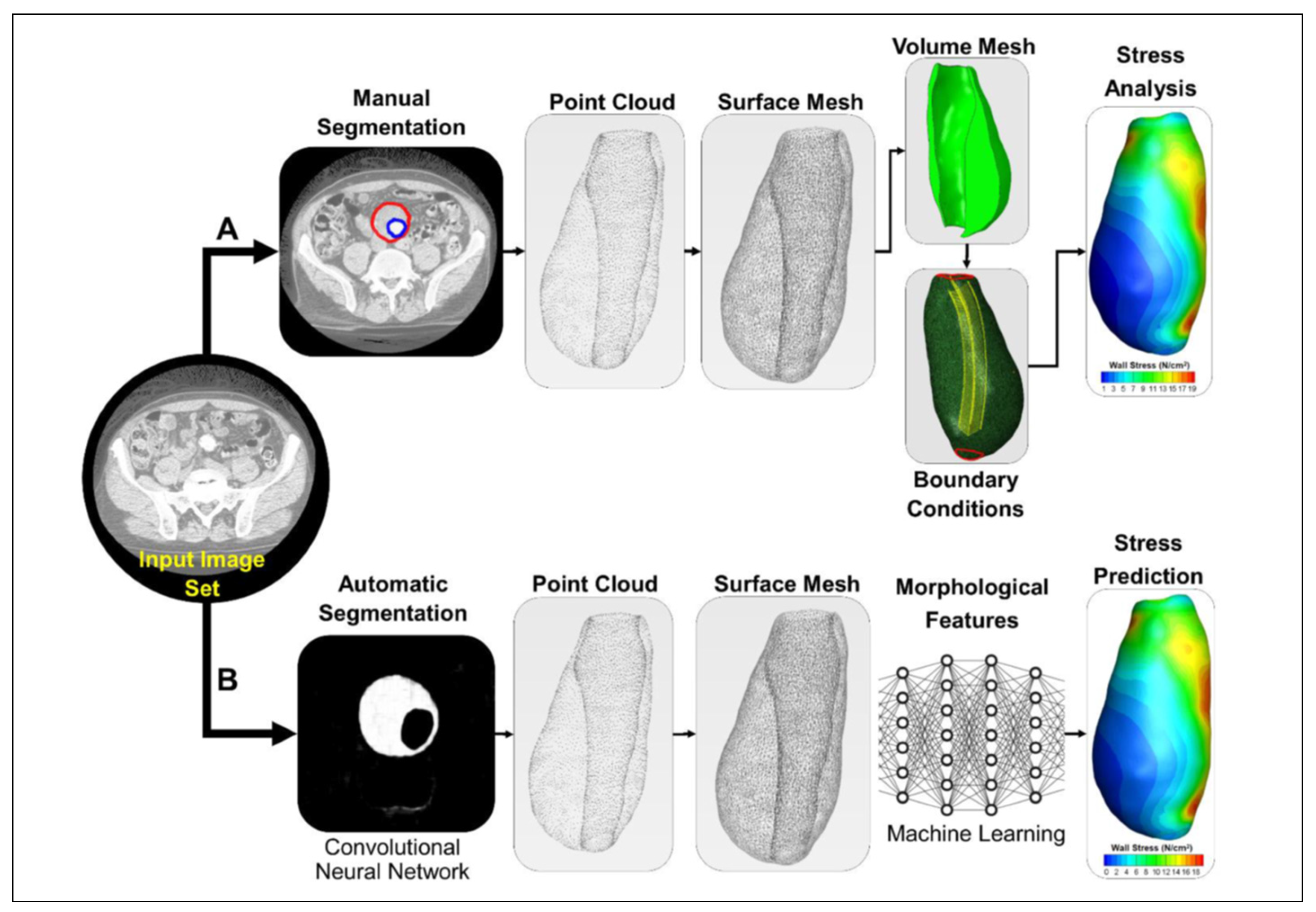
Figure 2.
Models of the patient (A) before and (B) after smoothing and cropping [55].
Figure 2.
Models of the patient (A) before and (B) after smoothing and cropping [55].
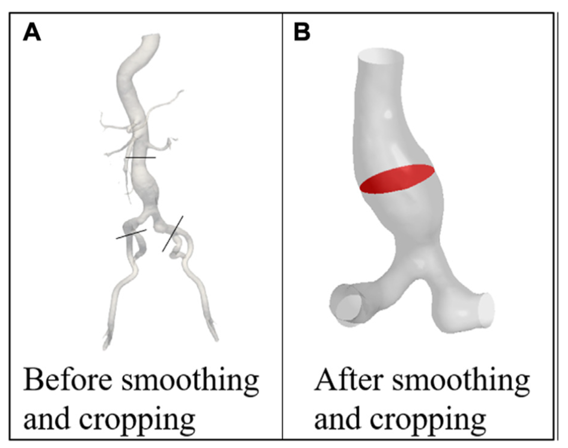
Figure 3.
3D reconstructions obtained from deep-learning based segmentation results for four different patients (A–D). The lumen is in blue, the aortic ILT/wall is transparent, and the celiac and renal arteries are shown in red and yellow, respectively.
Figure 3.
3D reconstructions obtained from deep-learning based segmentation results for four different patients (A–D). The lumen is in blue, the aortic ILT/wall is transparent, and the celiac and renal arteries are shown in red and yellow, respectively.
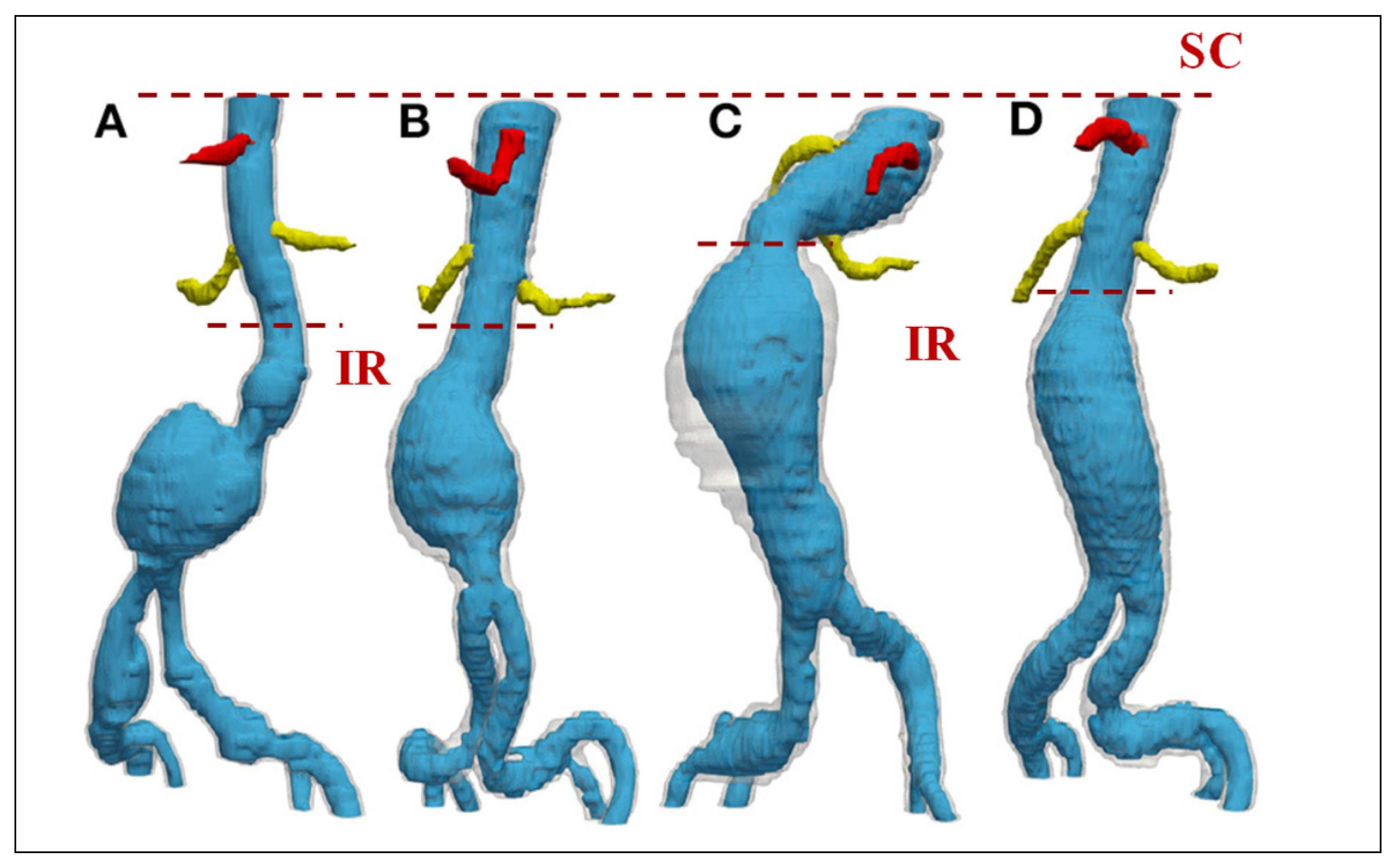
Figure 4.
Fluid and solid domains of AAA models with all boundaries.
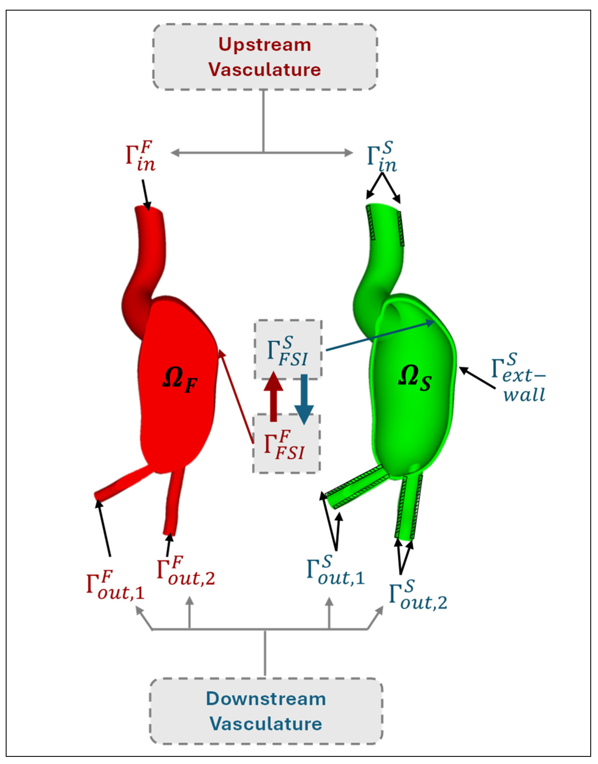
Figure 5.
The time-varying inlet velocity (obtained from the flow rate) and outlet pressure profile [109].
Figure 5.
The time-varying inlet velocity (obtained from the flow rate) and outlet pressure profile [109].
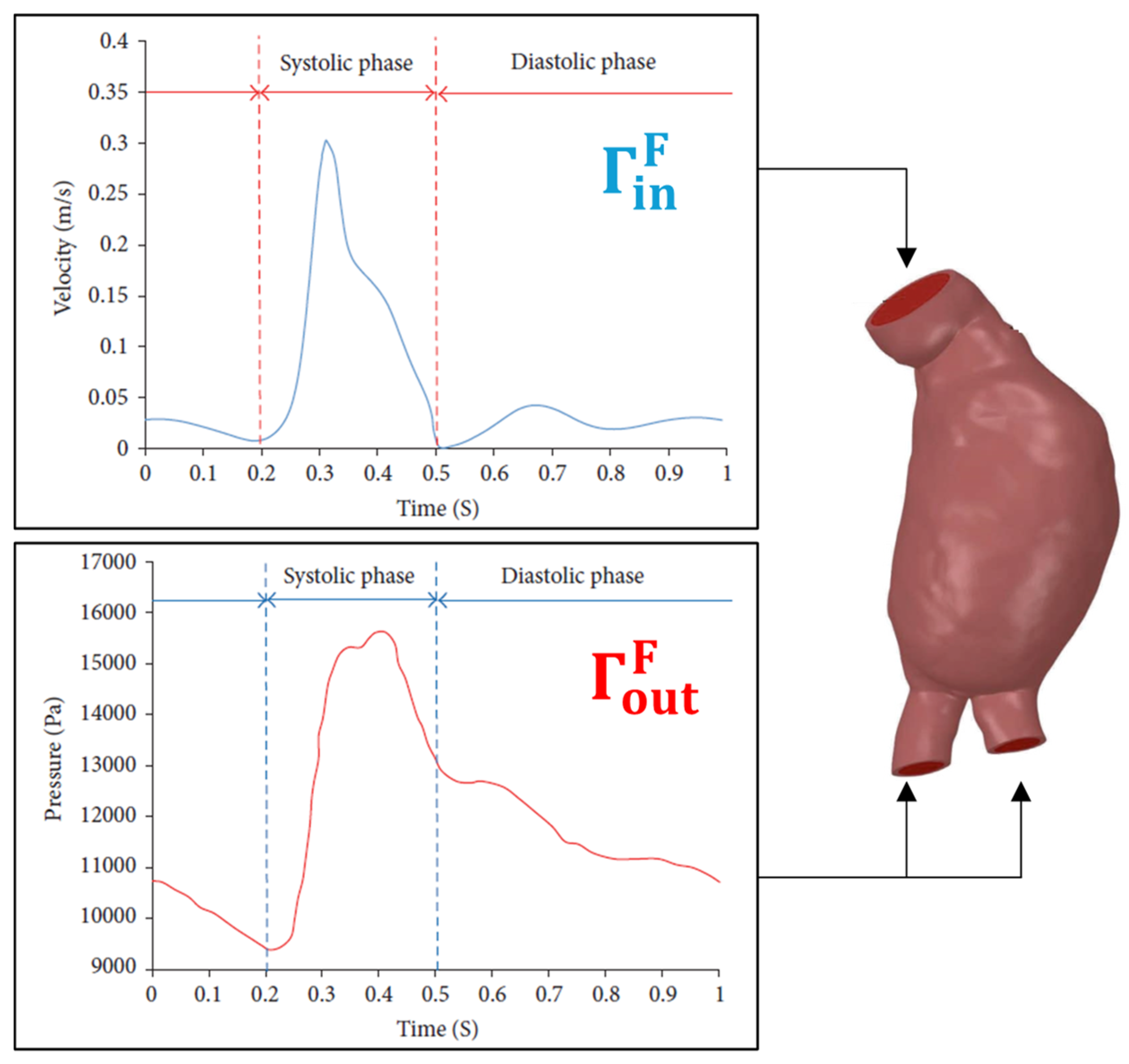
Figure 6.
(a) The time dependent flow rate at supraceliac (SC) and at infrarenal (IR) section; (b) The aorta branches at the downstream of SC: celiac trunk (CT), superior mesenteric (SM), left renal (LR), right renal (RR) and accessory right renal (ARR) arteries. The aorta branches at the downstream of IR: right and left internal and external arteries (RII, REI, LII, and LEI) [54].
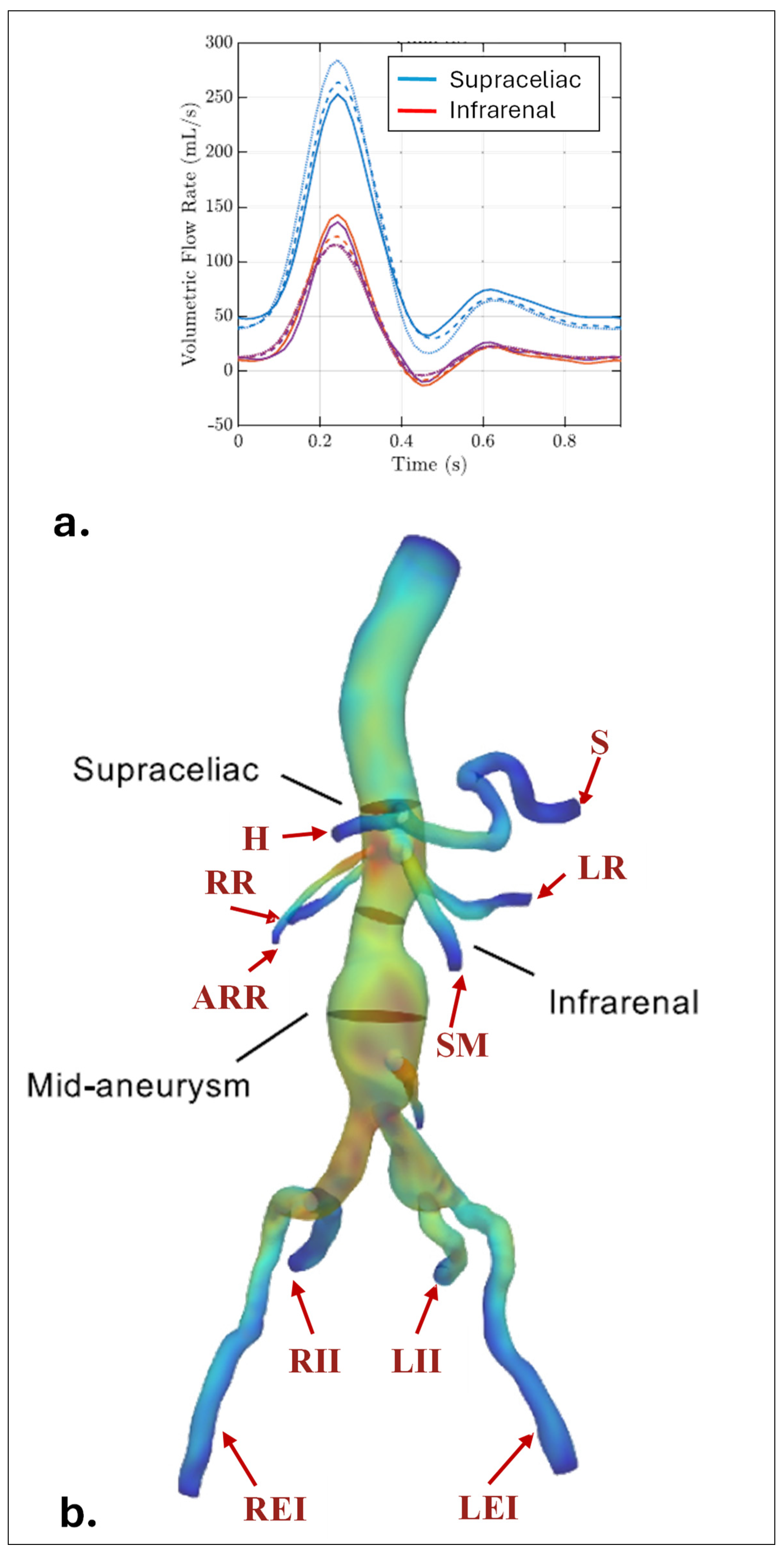
Figure 7.
The idealized velocity profiles provided at the inlet of AAA models. (a) Parabolic; (b) Plug (flat) and (c) Womersley profile [151].
Figure 7.
The idealized velocity profiles provided at the inlet of AAA models. (a) Parabolic; (b) Plug (flat) and (c) Womersley profile [151].
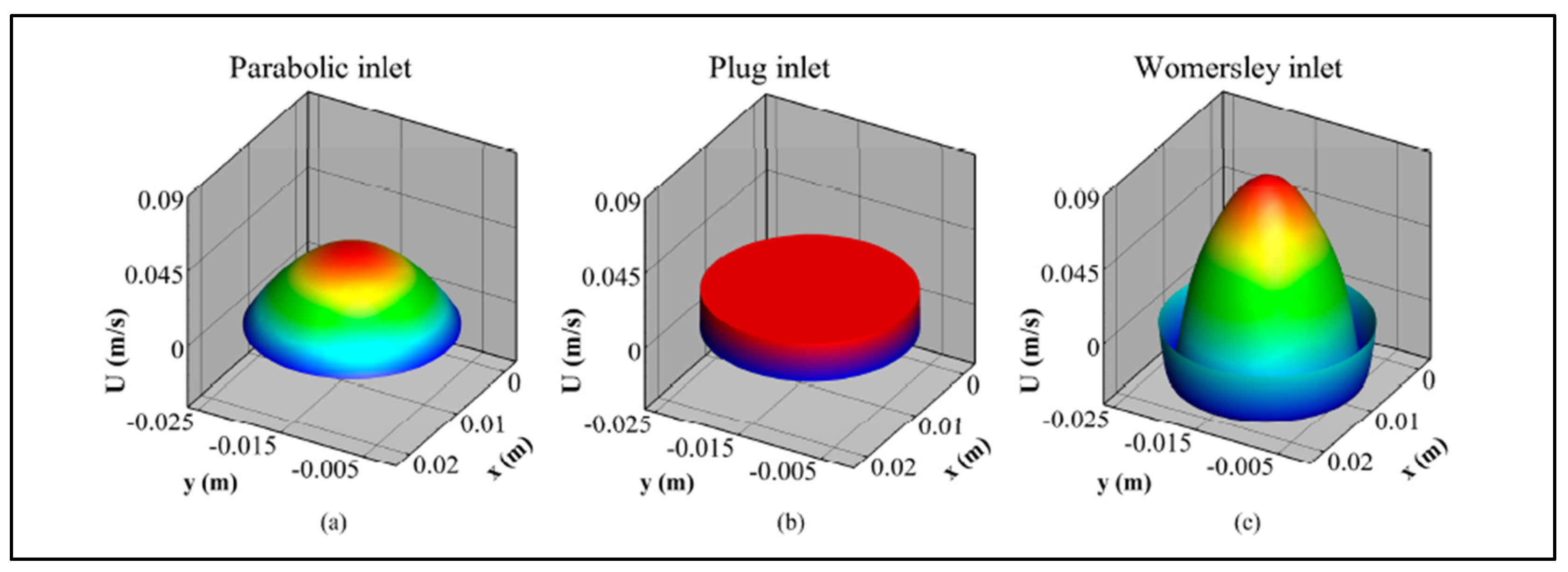
Figure 8.
WK models a. 2-element (RC), b. 3-element (RCR), and c. 4-element (RLC).
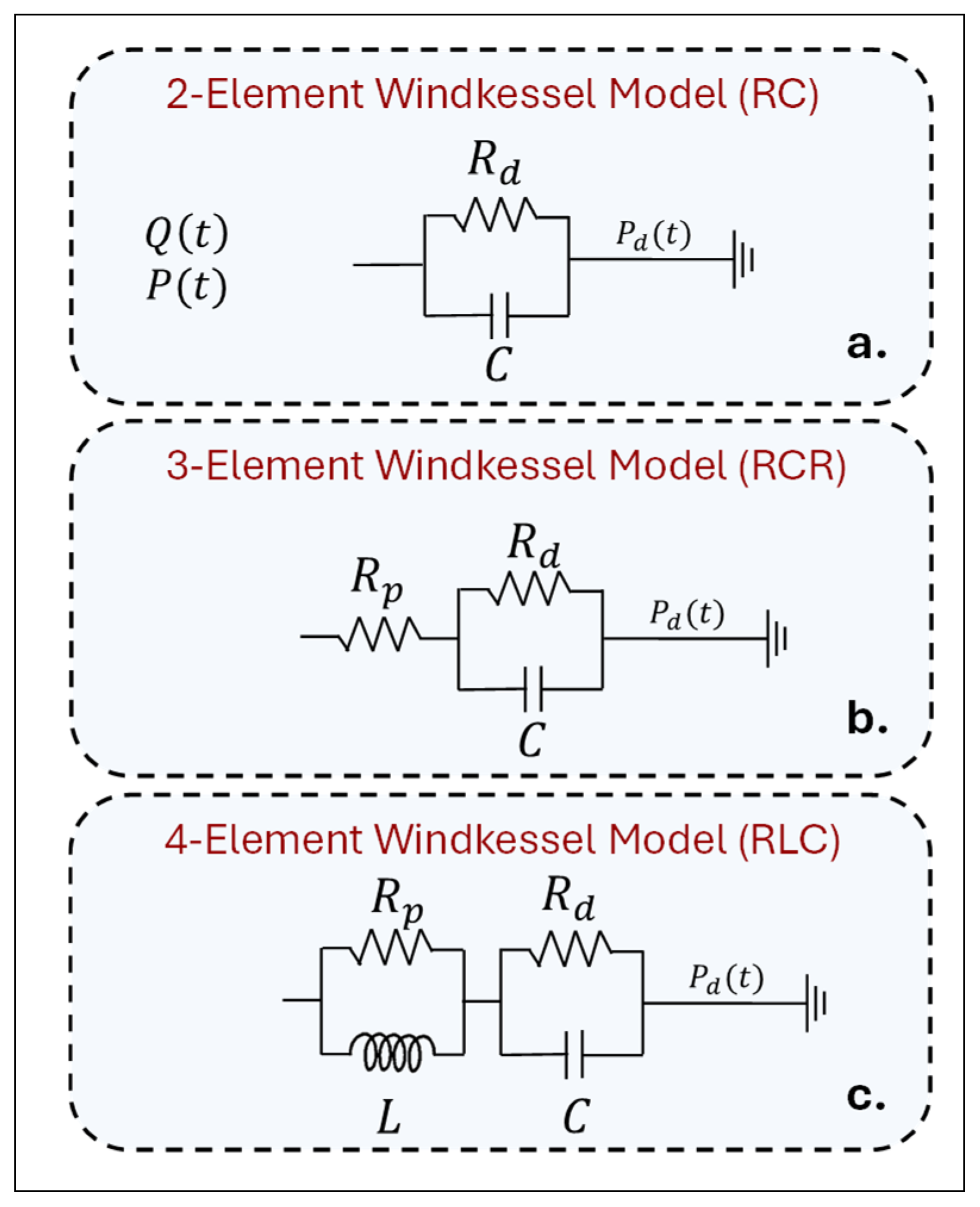
Figure 9.
3D domain of AAA and arterial branches coupled with separate 0D WK3 models at the outlets: S, H, SMA, LR, RR, LEI, LII, REI, and RII.
Figure 9.
3D domain of AAA and arterial branches coupled with separate 0D WK3 models at the outlets: S, H, SMA, LR, RR, LEI, LII, REI, and RII.
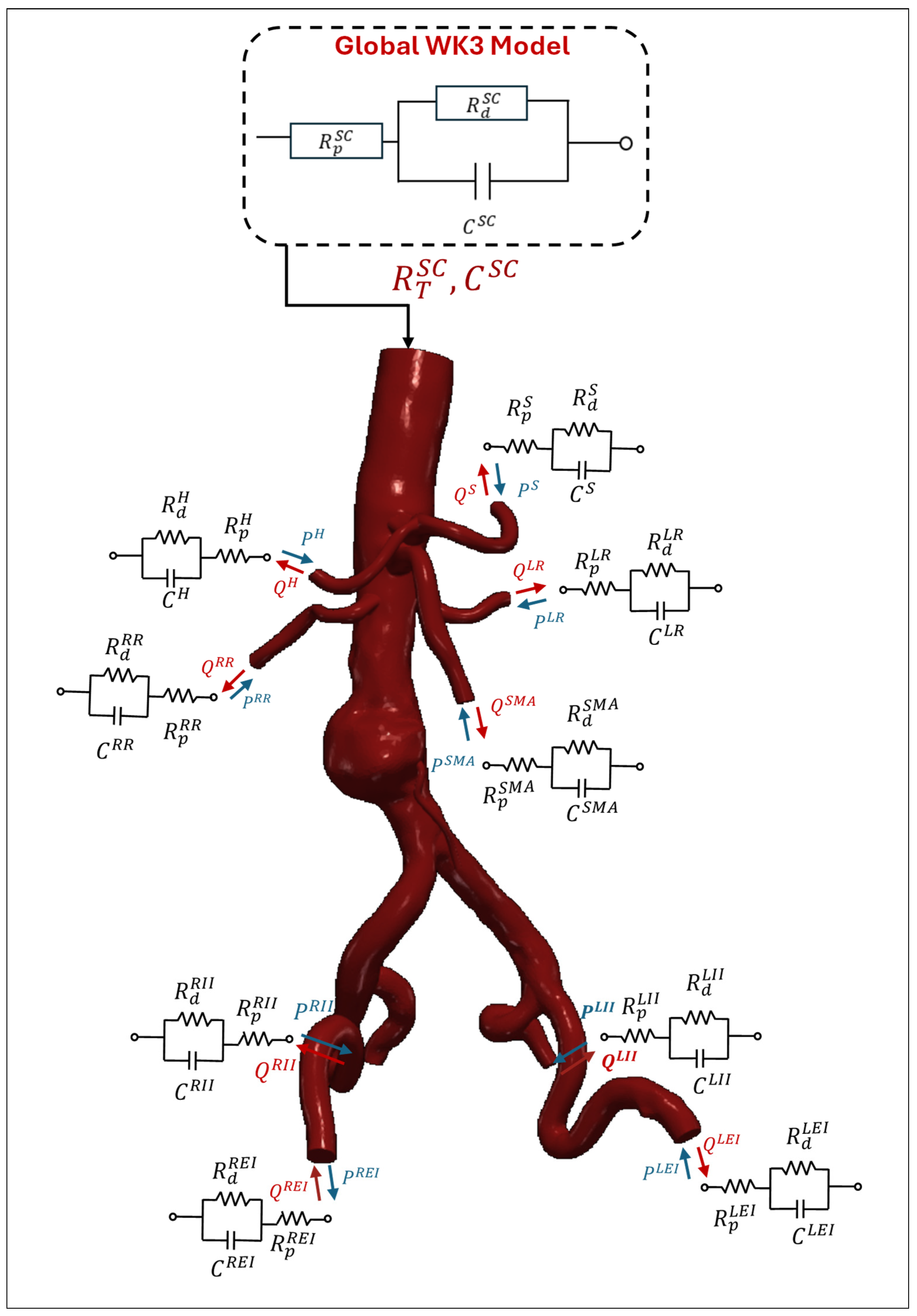
Figure 10.
The flowchart of global and local WK3 parameter estimation (using 1D equations and Murray’s Law) and coupling of 3D-0D domains [54].
Figure 10.
The flowchart of global and local WK3 parameter estimation (using 1D equations and Murray’s Law) and coupling of 3D-0D domains [54].
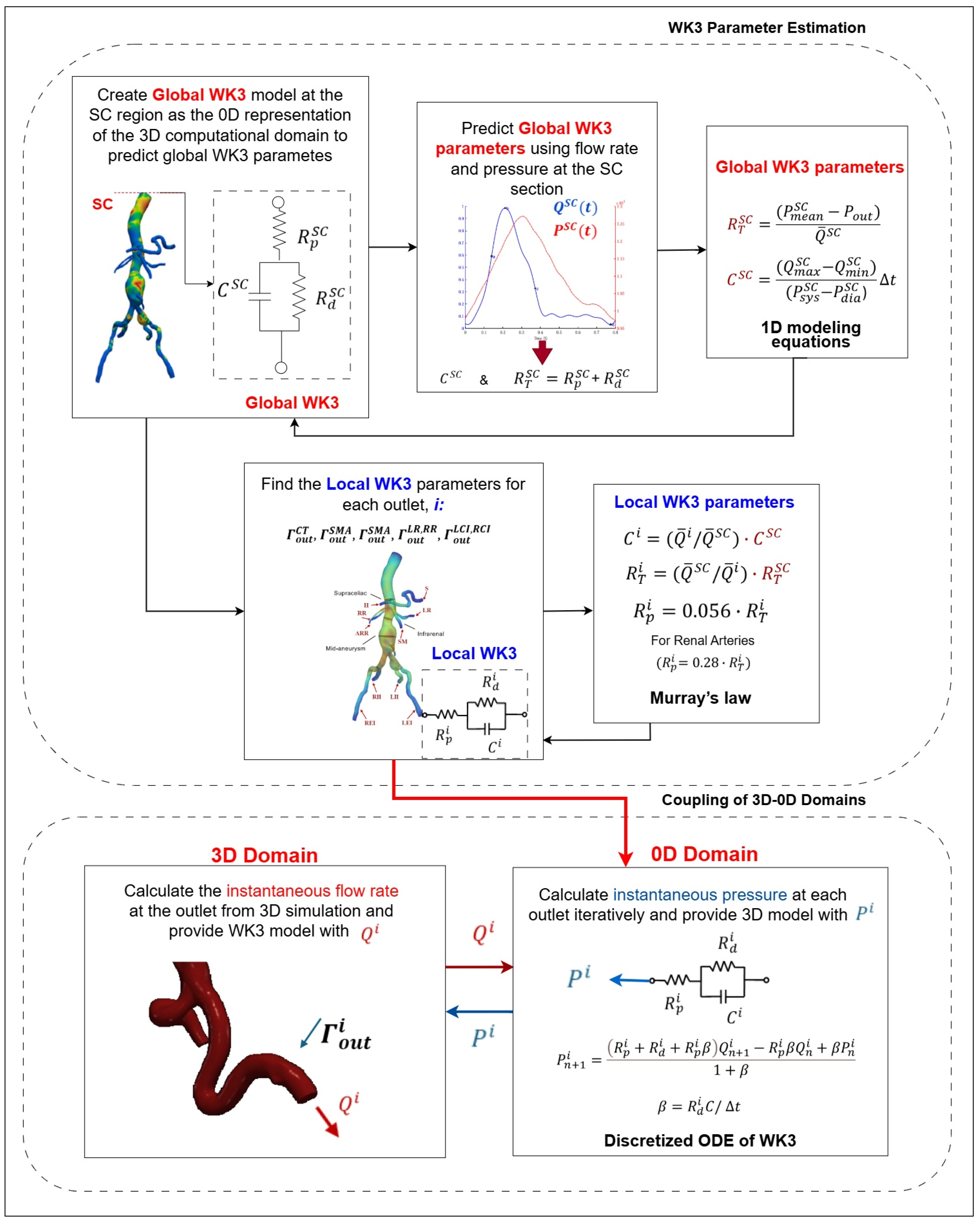
Figure 11.
Flowchart of the Resnet FCN architecture and AAA segmentation outputs [267].
Figure 11.
Flowchart of the Resnet FCN architecture and AAA segmentation outputs [267].
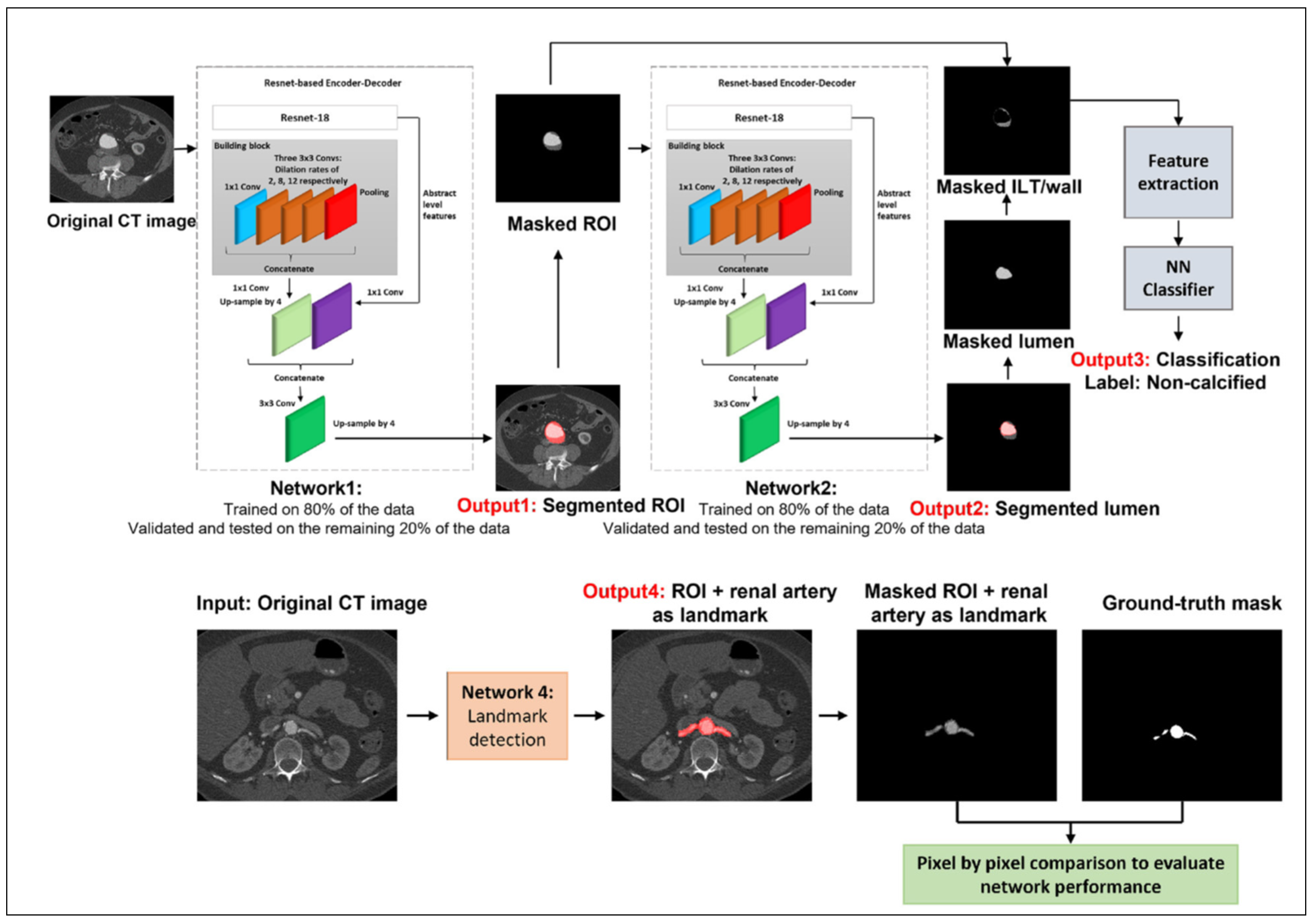
Figure 12.
Time-averaged wall shear stress (TAWSS, top) and oscillatory shear index (OSI, bottom) for a. E-uniaxial wall model, b. E-biaxial wall model, and c. rigid wall [54].
Figure 12.
Time-averaged wall shear stress (TAWSS, top) and oscillatory shear index (OSI, bottom) for a. E-uniaxial wall model, b. E-biaxial wall model, and c. rigid wall [54].
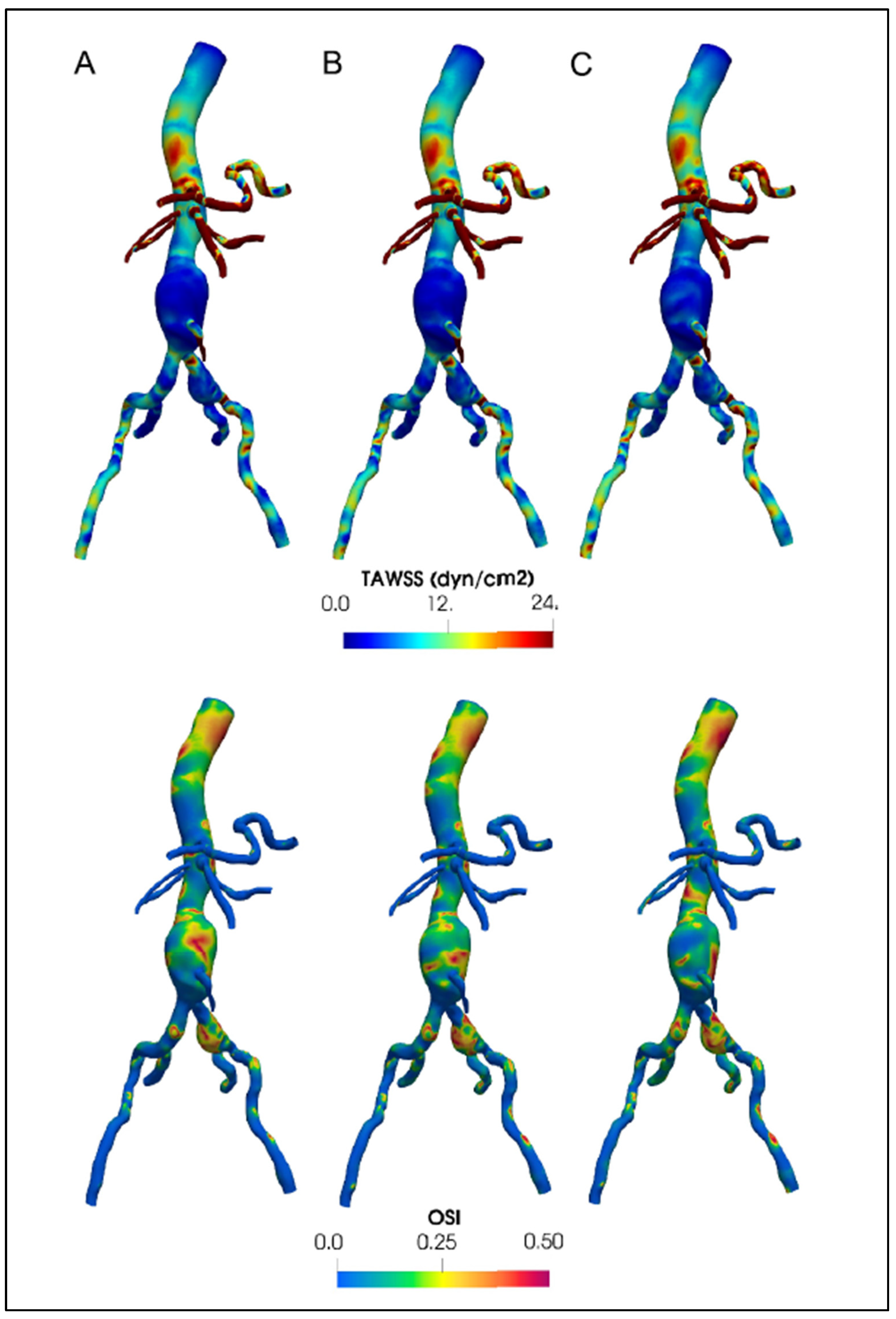
Table 1.
Boundaries of fluid and solid domains of AAA models.
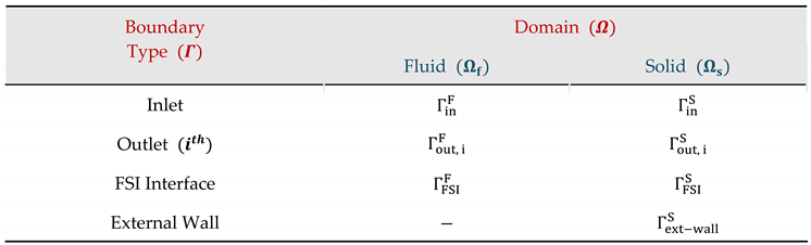 |
Table 2.
Flow split rates through branch arteries.
| Artery Branch | Flow Split |
| , | |
Disclaimer/Publisher’s Note: The statements, opinions and data contained in all publications are solely those of the individual author(s) and contributor(s) and not of MDPI and/or the editor(s). MDPI and/or the editor(s) disclaim responsibility for any injury to people or property resulting from any ideas, methods, instructions or products referred to in the content. |
© 2025 by the authors. Licensee MDPI, Basel, Switzerland. This article is an open access article distributed under the terms and conditions of the Creative Commons Attribution (CC BY) license (http://creativecommons.org/licenses/by/4.0/).
Copyright: This open access article is published under a Creative Commons CC BY 4.0 license, which permit the free download, distribution, and reuse, provided that the author and preprint are cited in any reuse.


