Preprint
Article

This version is not peer-reviewed.

Hybridly Explainable Verified Language Processing

A peer-reviewed article of this preprint also exists.

Submitted:

01 April 2025

Posted:

02 April 2025

Read the latest preprint version here

Abstract
The volume and diversity of digital information has led to a growing reliance on Machine Learning techniques, such as Natural Language Processing, for interpreting and accessing appropriate data. Among these techniques, vector and graph embeddings are used for representing data points, ranging from individual words to entire documents across multiple corpora. To retrieve this data, we need accurate similarity pipelines, to ensure we get relevant information from a given queried full-text. Current state-of-the-art does not guarantee this, as explainability is not certain. We demonstrate that our pipeline can achieve hybrid explainability, through combining graphs and logic to produce First-Order Logic representations, that are machine and human-readable via Montague Grammar. Preliminary results remark the effectiveness of the proposed approach in accurately capture full-text similarity by comparing our results with the cosine similarity derivable from sentence embedding generated by HuggingFace transformers.
Keywords: 
;  ;  ;  ;  ;  

1. Introduction

As the influence of Artificial Intelligence (AI) expands exponentially, so does the necessity for systems to be transparent, understandable, and above all, explainable [1]. This is further motivated by the untrustworthiness at the premises of Large Language Models (LLMs), which were not originally intended to provide reasoning mechanisms: as a result, when the system is asked about concepts upon which it was not originally trained, it tends to invent misleading information [2]. This is inherently due to the probabilistic reasoning embedded within the model [3] not accounting for inherent semantic contradiction implicitly derivable from the data through explicit rule-based approaches [4,5]. They do not consider reasoning by contradiction probabilistically with facts given as a conjunction of elements leads to iner unlikely facts [6,7]. All these consequences are self-evident in current state-of-the-art reasoning mechanisms and are currently referred to as hallucinations, which cannot be trusted to ensure verifiability of the inference outcome [8].
This paper walks on current literature evidence, showing that the best way to clear and detect inconsistencies within the data is to provide a rule-based approach to guarantee the effectiveness of the reasoning outcome [9,10] as well as by using logic-based systems [5,11]. Given the dualism between query and question answering [5], and given that query answering can be answered through structural similarity [12], we want first to address the research question of how to properly capture full-text sentence similarity containing potentially conflicting and contradictory data. Then, we assess the ability of current state-of-the-art learning-based approaches to do so, rather than solving the question problem directly, to solidify our findings. While doing so, we also address the question of whether such systems can capture logical-sentence meaning as well as retain spatiotemporal subtleties.
Vector embeddings, widely incorporated in these systems, lead to structural deficiencies in understanding given full-texts and ultimately destroy any possibility of properly explaining language. Neither vectors nor graphs independently can represent semantics and structure, as vectors lose structural information through averaging [13], while graph representations of sentences cannot usually convey similar structure for semantically similar sentences. Furthermore, they cannot faithfully express logical connectives: for the latter, none of the current graph-based representations uses nested nodes to represent a group of entities under a specific logical connector [14,15]. Metrics conceived for determining similarity are typically symmetric and, therefore, do not convey asymmetric notions of entailment, enhanced by this lack of logical connectives: e.g., if there is traffic in the city, then there is traffic also in the city centre, while the latter implication is in doubt. Vector-based systems use cosine similarity, which is trivially symmetric due to the use of the dot product. Graph-based similarity metrics are also symmetric, as the structural similarity is derived in terms of structural alignments across nodes and edges of interest [12]. Given the above, we cannot use structure or semantics alone to capture the full understanding of a given full-text; our code bridges the gap between them so it becomes possible.
Our previous work [16] has started to approach this problem, removing the black box and tunnelling in from a graph and logic point-of-view, which this paper continues to investigate. Explainability is vital in ensuring users’ trust in sentence similarity. The Logical, Structural and Semantic text Interpretation (LaSSI) (https://github.com/LogDS/LaSSI/releases/tag/v2.1, Accessed on 28 March 2025) pipeline takes a given full-text and transforms it into First-Order Logic (FOL), where we are returned with a representation that is both human and machine-readable, providing a way for similarity to be determined from full-text, as well as a way for individuals to reverse-engineer how this similarity was calculated. Similarity is then derived by reconciling such formulæ  into minimal propositions, which similarity is then addressed to derive the overall sentence similarity. By providing a tabular representation of both sentences, we can derive the confidence associated with the two original sentences, naturally leading to a non-symmetric similarity metric considering the possible worlds where sentences are valid.
While transformers can learn some semantical patterns occurring within full-text, they struggle with complex logic and nuances in natural language and do not fully grasp the semantic equivalence of active and passive sentences or perform multi-step spatiotemporal reasoning requiring common-sense knowledge. This is identified through clustering algorithms, highlighting how our proposed and transformer approaches differ in correctly clustering groups of full-text. Similarly, graph-based solutions, while effective in representing structure and relationships, face challenges in graph construction and handling the ambiguity of natural language. Both approaches have limitations in capturing the logical implications in spatiotemporal contexts.
Our pipeline aims to leverage these limitations: this is achieved through key pre-processing steps that acknowledge structure properly, by contextualising semantics to rewrite a given graph and generate a formula. Consequently, given sentences with equivalent meaning that produce structural disparate graphs, we get equal formulæ . An intermediate graph representation is constructed before this formula creation, where we execute a topological sort on our initial graph, so that we encompass recursive sentence structure possibly contained within full-texts, perform Multi-Word Entity Unit (MEU) recognition where we identify context behind entities within sentences, and incorporate these within properly defined properties of a sentence kernel. Our experiments show that these conditions cannot be captured with semantics alone.
This paper addresses the following research questions through both theoretical and experiment-driven results:
RQ №1
Can transformers and graph-based solutions correctly capture the notion of sentence entailment? Theoretical results (Section 4.1) remark that similarity metrics mainly considering symmetric properties of the data are unsuitable for capturing the notion of logical entailment, for which we at least need quasi-metric spaces or divergence measures. This paper offers the well-known metric of confidence [17] for this purpose and contextualises it within logical-based semantics for full-text.
RQ №2
Can transformers and graph-based solutions correctly capture the notion of sentence similarity? The previous result should implicitly derive the impossibility of deriving the notion of equivalence as entailment implies equivalence through if-and-only-if but not vice versa, we aim at deriving similar results through empirical experiments substantiating the claims in specific contexts. We then design datasets addressing the following questions:
(a)
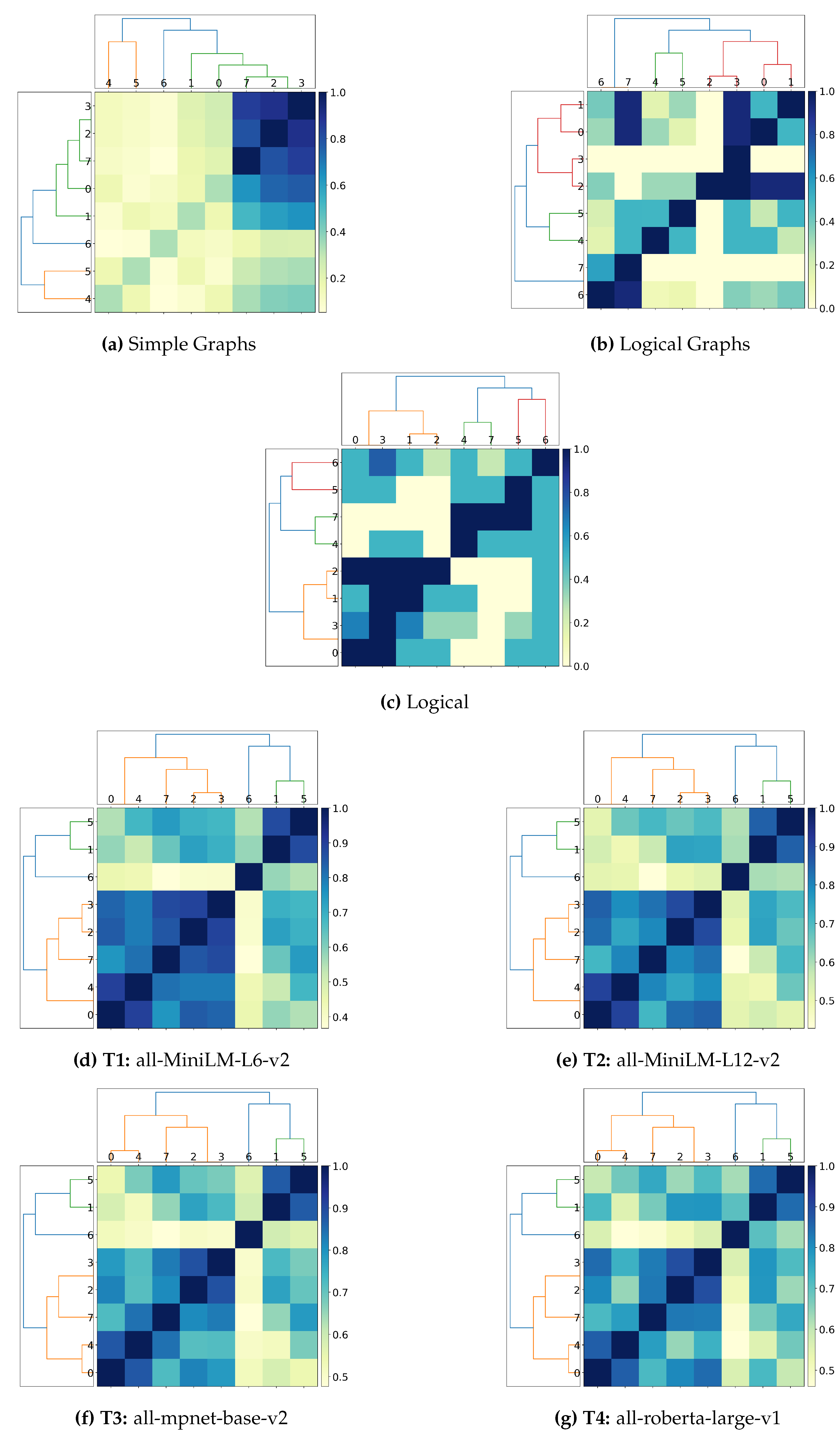
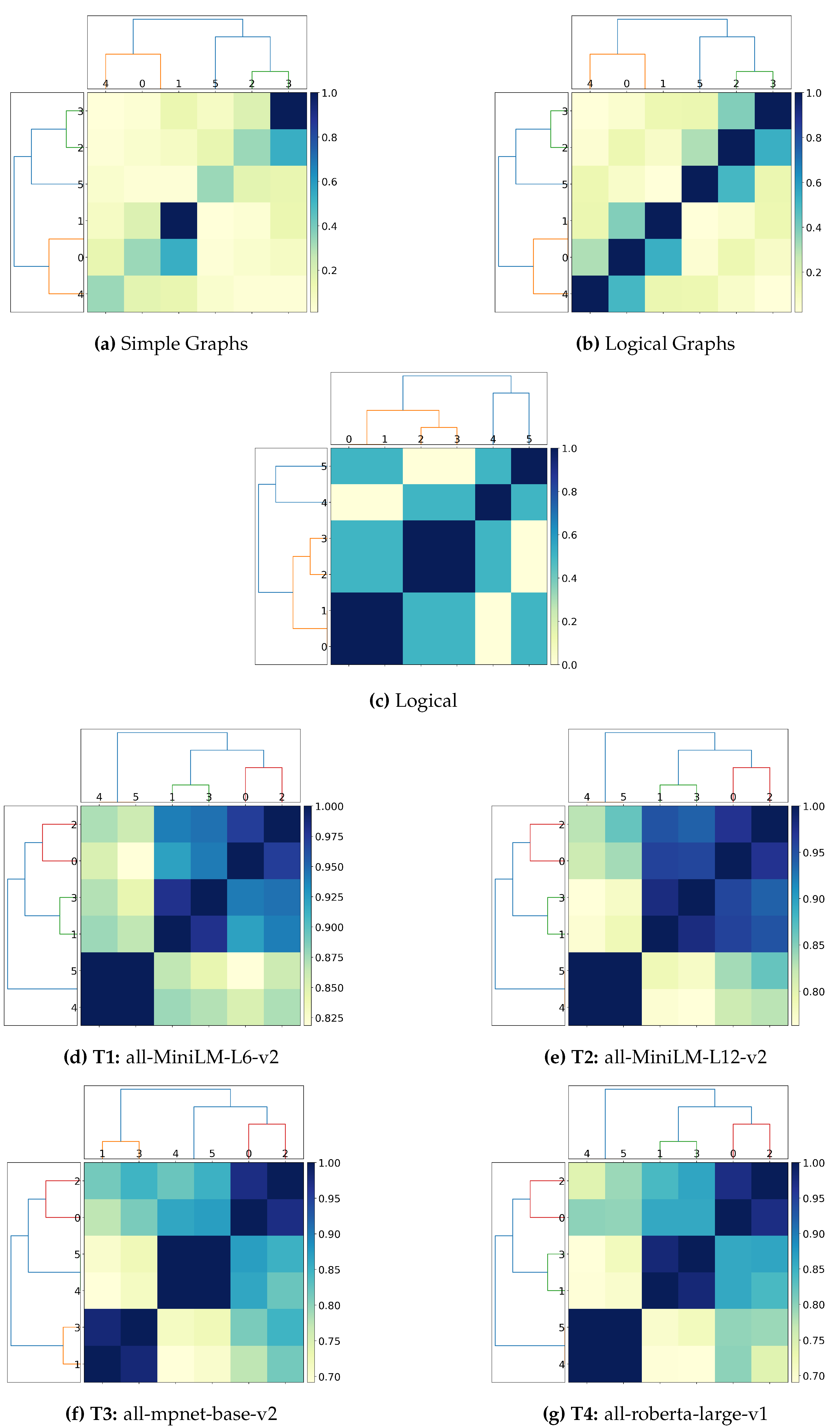
Can transformers and graph-based solutions capture logical connectives? Current experiments (Section 4.2.1) show that vector embeddings generated by transformers cannot adequately capture the information contained in logical connectives, which can only be considered after elevating such connectives as first-class citizens (Simple Graphs vs. Logical Graphs). Furthermore, given the experiments’ outcome, vector embedding likely favours entities’ position in the text and discards logical connectives occurring within the text as stop words.
(b)
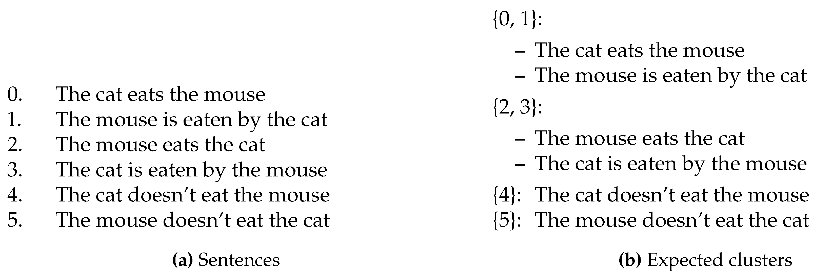
Can transformers and graph-based solutions distinguish between active and passive sentences? Preliminary experiments (Section 4.2.2) show that structure alone is insufficient to implicitly derive semantic information, which requires extra disambiguation processing to derive the correct representation desiderata (Simple and Logical graphs vs. Logical). Furthermore, these experiments reaffirm the considerations on the positionality and the stop word from the previous research question, as vector embeddings cannot clearly distinguish between active and passive sentences (Logical vs. Transformer-based approaches).
(c)
Can transformers and graph-based solution correctly capture the notion of logical implication (e.g.) in spatiotemporal reasoning? Spatiotemporal reasoning requires specific part-of and is-a reasoning that is, to the best of our knowledge and at the time of the writing, unprecedented in current literature on logical-based interpretation of the text. Consequently, we argue that these notions cannot be captured by embeddings alone and by graph-based representations using merely structural information, as this requires categorising the logical function of each entity occurring within the text as well as correctly addressing the interpretation of the logical connectives occurring (Section 4.2.3).
RQ №3
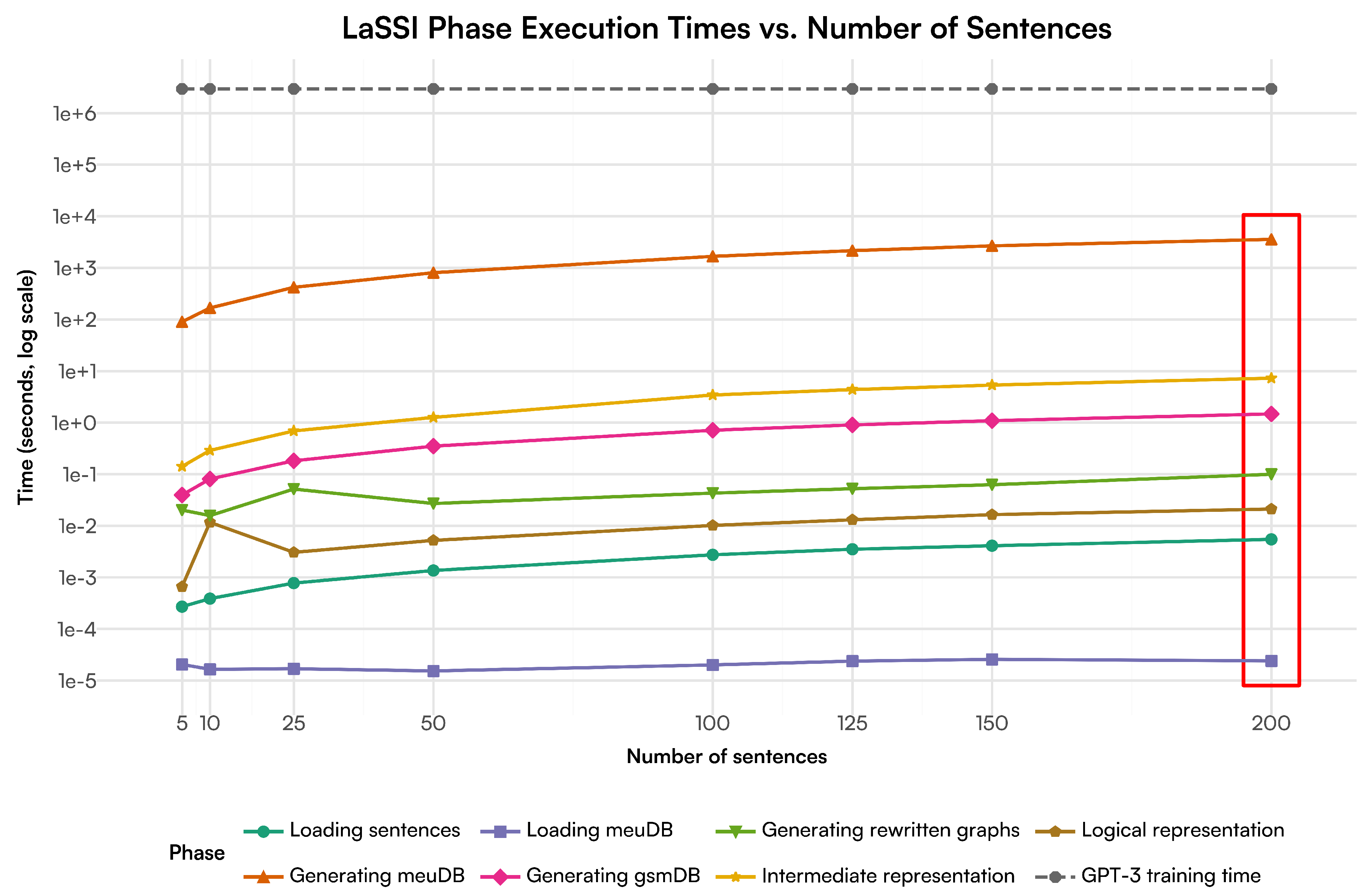
Is our proposed technique scalable? Benchmarks over a set of 200 sentences retrieved from sentences occurring within ConceptNet [18] (Section 4.3) remark that our pipeline works in at most linear time over the number of the sentences, thus remarking the optimality of the envisioned approach.
RQ №4
Can a single rewriting grammar and algorithm capture most factoid sentences? Our discussion (Section 5) remarks that this preliminary work improves over the sentence representation from our previous solution, but there are still ways to improve the current pipeline. We also argue the following: given that training-based systems are also based on annotated data to correctly identify patterns and return correct results (Section 2.2), the output provided by training-based algorithms can be only as correct as the ability of the human to consider all the possible cases for validation. Thus, rather than postulating the need for training-based approaches in the hope the algorithm will be able to generalise over unseen patterns within the data, we speculate the inverse approach should be investigated. This is because the only possible way to achieve an accurate semantic representation of the text is through accurate linguistic reconstruction using derivational-based and pattern-matching approaches (Section 2.3).
The paper is then structured as follows: after contextualising our attempt of introducing for the first time verified AI within the context of Natural Language Processing (NLP) through explainability (Section 2.1), we mainly address current NLP concepts for conciseness purposes (Section 2.2). Then, we motivate that our pipeline achieves hybrid explainability by showing its ability to provide a priori explanations (Section 3.2), from which the text is enriched with contextual and semantic information, ad hoc explanations (Section 3.3), through which the sentence is now represented in a verifiable representation (be that a vector, a graph, or a logical formula), and a final human-understandable ex post explanation (Section 3.4), through which we boil down the desired textual representation generated by the forthcoming phase into a similarity matrix. This helps to better appreciate how the machine can interpret the similarity of the text. After providing an in-depth discussion on the improvements over our previous work (Section 5), we draw our conclusions

2. Related Works

2.1. General Explainable and Verified Artificial Intelligence

A recent survey introduced the notion of verified AI [19], through which we seek greater control by exploiting reliable and safe approaches to derive conclusions over the data. This survey also remarked that, at the time of the writing, providing a truly verifiable approach of NLP is still an open challenge and was not resolved with current techniques. As the same survey also observes that real verification cannot exclude a logical representation of the data of interest, more recent approaches [1] have been attempting to revive previous non-training-based approaches showing the possibility of representing a query out of a full-sentence by mainly exploiting semantic parsing [20]. The more recent approach also enables sentence representation in logical format rather than ensuring a SQL representation of the text. As a result, the latter can also be easily rewritten and used for inference purposes. Notwithstanding the former, the authors did not encompass all the rewriting steps required to capture different linguistic functions and categorise their role within the sentence, as we are doing differently within the present paper. Furthermore, while authors in [1] already attempt to answer questions, our paper does a preliminary step back, for which we first test the suitability of our proposed approach to derive correct sentence similarity from the logical representation, after which we will then tackle the possibility of using logical-based representations also to answer questions. While doing so, we also ensure the correct capturing of multi-word entities occurring within the text while differentiating between the main entities from the properties specifying them.
Our latest work also remarks on the possibility of achieving verification when twinned with explainability in a way that makes the data understandable to both humans and machines [21]. This identifies three distinct phases to be considered as prerequisites for achieving good explanations: first, within the first a propri explanation, unstructured data should achieve a higher structural representation level by deriving additional contextual information from the data and environment. After this, the ad hoc explanation should provide an explainable way through which a specification is extracted from the data, where provenance mechanisms help trace all the data processing steps. If represented as a logical program, the specification can also ensure both human and machine understandability by being represented in an unambiguous format. Last, the ex post phase should further refine the previously generated specifications by achieving better and more fine-grained explainability. Therefore, we can derive even more accessible results and ease the comparisons between models, while enabling their comparison with other data. Our methodological section will then reflect these phases.

2.2. Natural Language Processing

Part of Speech (POS) tagging algorithms work as follows: each word in a text (corpus) is marked up as belonging to a specific part of speech, which is based on the term’s definition and context [22]. Words can be then categorised as nouns, verbs, adjectives, or adverbs. In Italian linguistics (Section 2.3.1), this phase is referred to as grammatical analysis of a sentence structure and belongs to the most fine-grained analysis. As an example for POS tags, we can retrieve these initial annotations for the sentence, “Alice plays football” from Stanford CoreNLP [23], which would identify “Alice” as a proper noun (NNP), “plays” as a verb (VBZ - present tense, third person singular) and “football” as a noun (NN), thus determining the subject-verb-object relationship between these words.
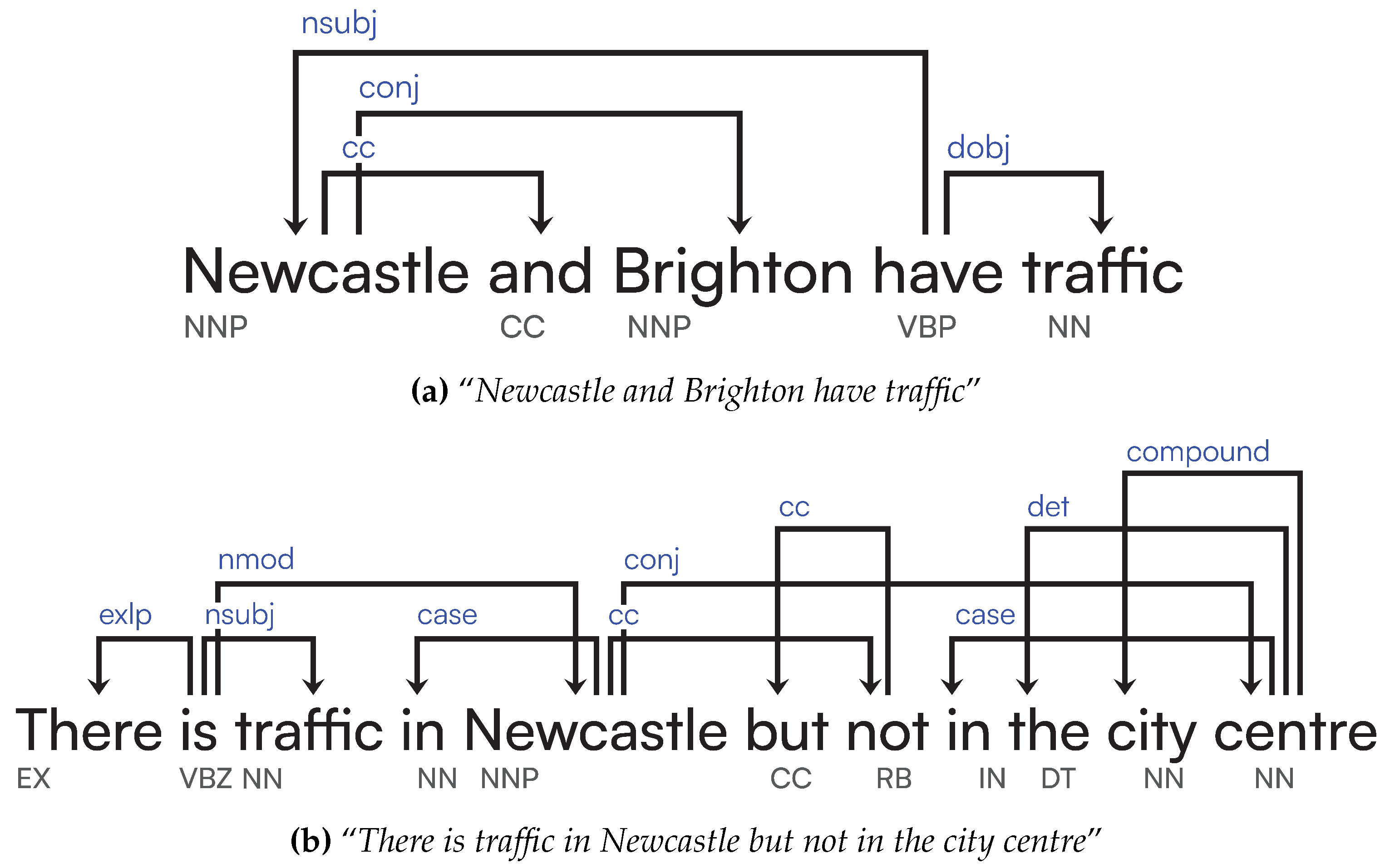
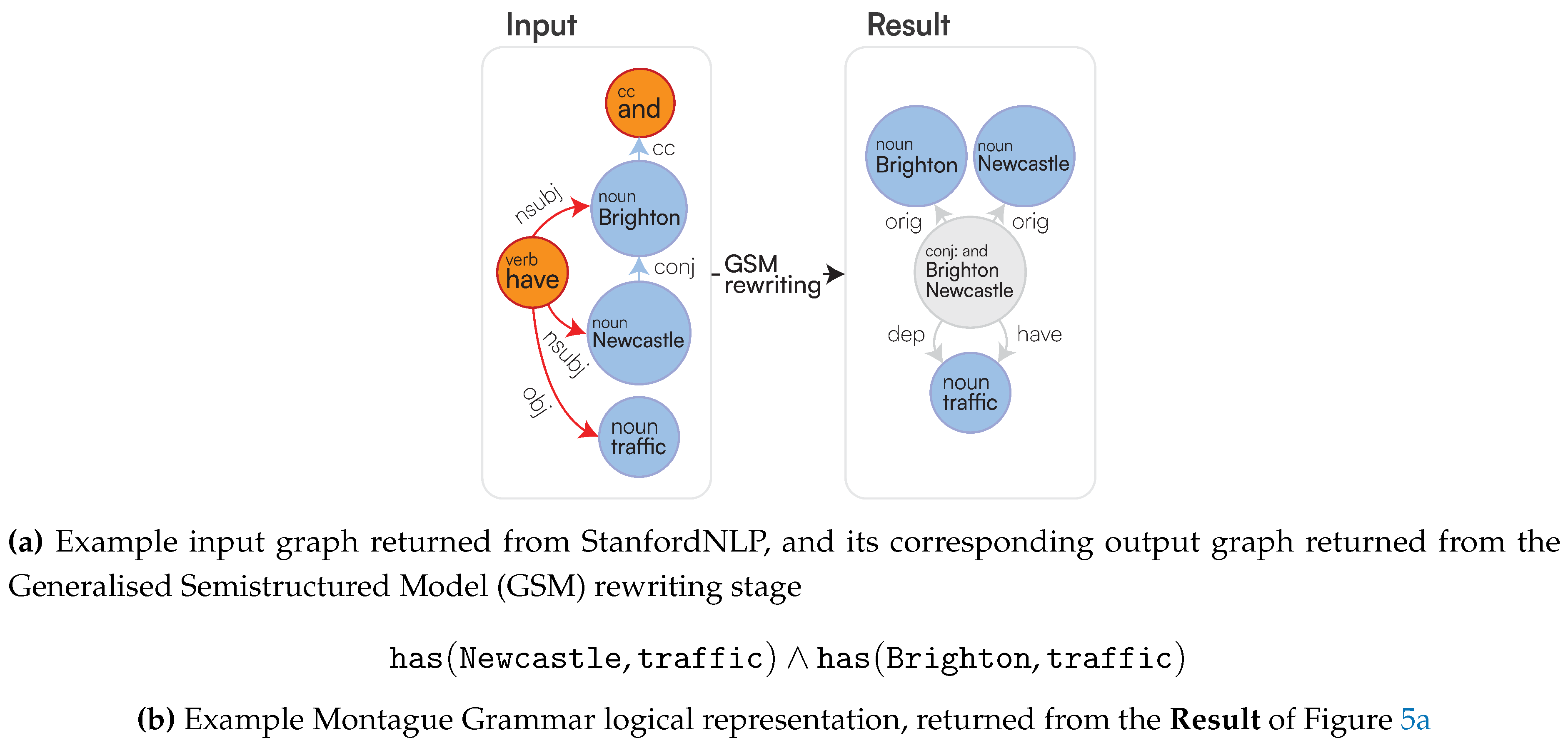
Dependency parsing refers to the extraction of language-independent grammatical functions expressed through a minimal set of binary relationships connecting POS components within the text, thus allowing a semi-structured, graph-based representation of the text. These dependencies are beneficial in inferring how one word might relate to another. For example, a conj [24] dependency represents a conjunct, which is a relation between two elements connected by a cc [25]: a coordination determining what type of group these elements should be in. We can extract these ud, also through Stanford CoreNLP, whereby we are returned annotations for each word in the sentence, giving us relationships and types. As shown in Figure 1, relationships are labelled on the edges, and types are labelled underneath each word. Looking at Figure 1, Newcastle and traffic are all children of have, through nsubj and dobj relationships respectively. Types are determined from POS tags [26], so we can identify that have is a verb as it is annotated with VBP (a verb of the present tense and not third-person singular). The nsubj relation stands for the nominal subject, and the dobj is the direct object, thus meaning that Newcastle acts upon traffic by having the traffic. Brighton is also a child of Newcastle through a conj relation, and Newcastle has a cc relation to and, inferring these two subjects are related. Consequently, if we know Newcastle has traffic, then it holds that Brighton does as well. These POS tags also indicate Newcastle and Brighton are proper nouns as they have NNP types.
Capturing syntactical features through training is challenging. Neural Network (NN)-based approaches are not proficient in precisely capturing relationships within text, as they fall down the same limitations as in vector-based representations of sentences. Figure 1 shows how AI struggles with understanding negation from full-text, this sentence was fed into a natural language parser [27] and the result shows no sign of a neg (negated) dependency, despite “but not” being contained within the sentence. Still, we can easily identify and fix these issues before returning the Dependency Graph (DG) to our LaSSI pipeline.

2.3. Linguistics and Grammatical Structure

The notion of systematic and rule-based characterisation of human languages pre-date modern studies on language and grammar: Aṣṭādhyāyī by Pāṇini utilises a derivational approach to explain the Sanskrit language, where speech is generated from theoretical, abstract statements created by adding affixes to bases under specific conditions [28]. This further supports the idea of representing most human languages in terms of grammatical derivational rules, from which we can identify the grammatical structure and functions of the terms occurring in a piece of text [29]. This induces the recursive structure of most Indo-European languages, including English, which should be addressed to better analyse the overall sentence structure into its minimal components.
Take the example in Figure 2; this could continue infinitely as a consequence of recursion in language due to the lack of an upper bound on grammatical sentence length [30]. Given the possibility of injecting the full-text with semantic annotations, these can be further leveraged to derive a logical representation of the sentence [1].
Richard Montague developed a formal approach to natural language semantics, which later became known as Montague Grammar (MG), where natural and formal languages can be treated equally [31] to allow for the rewriting of a sentence in a logical format by assuming the possibility of POS tagging. MG assumes languages can be rewritten given their grammar [32], preserving logical connectives and expressing verbs as logical predicates. MG then provides a set of rules for translating this into a logical form; for instance, a sentence (S) can be formed by combining a noun phrase ( N P ) and a verb phrase ( V P ); we can also find the meaning of a sentence obtained by the rule S : N P V P , whereby the function for N P is applied to the function V P . MG uses a system of types to define the different kinds of expressions and their meanings. Some common types include t, denoting a term (a reference to an entity), and f, denoting a formula (a statement that can be true or false). The meaning of an expression is obtained as a function of its components, either by function application or by constructing a new function from the functions associated with the component. This compositionality makes it possible to assign meanings reliably to arbitrarily complex sentence structures, we can then extract predicate logic from this, so the sentence: “Alice plays football” becomes: play(Alice, football).
However, MG only focuses on the logical form of full-text, overlooking the nuances of context and real-world knowledge. For example, does “Newcastle” refer to “Newcastle-upon-Tyne, United Kingdom”, “Newcastle-under-Lyme, United Kingdom”, “Newcastle, Australia” or “Newcastle, Northern Ireland”; without an external Knowledge Base (KB) or ontology, it is difficult to determine which of these it could be, unless the full-text provides relevant explicit information. Therefore, providing a dictionary of possible matches for all words in the sentence can significantly improve the MEU recognition, meaning known places, people and organisations can be matched to enhance the understanding of the syntactic structure of a given full-text. At the time of the writing, no Graph Query Language (GQL) can combine semantic utilities related to entity resolution alongside with more structural rewriting of the sentence. Therefore, this forces us to address minimal sentence rewriting through GQLs, while considering the main semantic-driven rewritings in our Python code base provided above, where all of these are accounted for.

2.3.1. Italian Linguistics

Not all grammatical information can be captured from MG alone: we can identify words that are verbs and pronouns, however these can both be broken down into several sub-categories that infer different rewriting that is not necessarily apparent from the initial structure of the sentence. For instance, a transitive verb is a verb that can take a direct object, “the cateatsthe mouse”, so when rewriting into the logical form we know that a direct object must exist, therefore becoming: eat(cat, mouse), where eat is acting on the mouse. However, if the verb is intransitive, “goingacross the street”, then the logical form must not have a direct object and is thus removed, as the target does not reflect the direct object. Therefore, this sentence becomes: go(?)[(SPACE:street[(det:the), (type:motion through place)])], as go does not produce an action on the street. The target is removed from the rewriting to reflect the nature of intransitive verbs. All these considerations are not accounted for in current NLP pipelines for Question Answering (QA) [1], where merely simple binary relationships are accounted for, and the logical function of the part of speech components is not considered.
In Italian linguistics, the examination of a proposition, commonly referred to as logical analysis, is the process by which the components of a proposition and their logical function within the proposition itself are recognised [33]. In this regard, this analysis recognises each clause/sentence as a predicate with its (potentially passive) subject, where we aim to determine the function of every single component: the verb, the direct object, alongside any other “indirect complement” which can refer to either an indirect object, adverbial phrases, or to a locative [34]. This kind of analysis aims at determining what type of purpose the text is communicating and characterises each adverbial phase by the kind of information being conveyed (e.g., limitation, manner, time, space) [33]. This significantly differs from the POS Tagging of each word appearing in a sentence (Figure 1), via which each word is associated to a specific POS (adjective, noun, verb), as more than just one single word could participate in providing the same description. Concerning Figure 1, both Newcastle and Brighton from the first sentence are considered part of the same subject, Newcastle and Brighton, while in Newcastle is recognised as a Space adverbial of time Stay in place, given the preposition it and the verb is not indicating a motion rather than a state; implicitly, this analysis considers “but not in the city centre” as a separate coordinate clause, where “There is (not) traffic” is subsumed from the main sentence. We argue that the possibility of further extracting more contextual knowledge from a sentence via logical analysis tagging helps the machine to categorise the text’s function better, thus providing both machine and human-readable explanations. Our paper recognises the linguistic functions of the sentence as outlined in Table 1 and, given the missing of such characterisation from the English language, we freely exploit the characterisation found in Italian linguistics and contextualise this to the English language.
To distinguish between Italian and English linguistic terminology, we are referring to the characterisation of such elements of the sentence beyond the subject-verb-direct object characterisation as Logical Functions.

3. Materials and Methods

Let α and β be full-text sentences: in this paper, we consider only factoid sentences that can at most represent existentials, expressing the omission of knowledge to, at some point, be injected with new, relevant information. τ represents a transformation function, whereby the vector or logical representations are denoted as τ ( α ) = A and τ ( β ) = B for α and β respectively. From τ, we want to derive a logical interpretation through φ from τ while capturing the common sense from the text. We then need a binary function φ τ expressing this for each transformation τ (Section 4.1). Figure 3 showcases the entire pipeline providing such transformation phases.

3.1. Extensions to the Generalised Graph Grammar Language and Graph Grammar Rewriting Rules for ud

To improve the final logical rewriting, the Generalised Graph Grammar (GGG) language demonstrated in [35] was extended to capture more information: in particular, now newly created nodes can copy properties from newly created or already-existing nodes, as well as supporting better node variable matching and updates. Some ud [36] which were not accounted for previously are now considered in our graph grammar rewriting rules: parataxis and compound_prt. There was an issue whereby if an entity contained multiple case properties, they would not all appear in the node’s properties, due to the properties being key-value associations, where the key can only take one value. To overcome this, the case property keys are labelled as their float positions occurring within the sentence. For example for the sentence, “It is busy in Newcastle”, our case property “in”, is at the 4th position, so “Newcastle” would have a property {4:in}. This also means that more information is retained within the rewriting, as we can identify whether this property precedes or proceeds the given entity, which is not pertinent at the moment, but is discussed in Section 6 on how it will improve the pipeline in the future.

3.2. A Priori Explanation

In the a priori explanation phase, we aim to enrich the semantic information for each word (Section 3.2.1), to subsequently recognise multi-word entities (Section 3.2.2) with extra information (i.e., specifications, Section 3.2.3) by leveraging the former. This information will be used to pair the intermediate syntactic and morphological representation of the sentence achieved through subsequent graph rewritings (Section 3.3) with the semantic interpretation derived from the phase narrated within the forthcoming subsections.
The main data structure conveyed for nesting dependant clauses represented as (kernel) relationships occurring at any recursive level of the sentence is the Singleton. This also represents the atomic representation of an entity (Section 3.2.1), thus including each single word of a multi-word entity (Section 3.2.2). It is defined with attributes: id, named_entity, properties, min, max, type, confidence, and kernel. When the latter field is none, properties mainly refer to the entities, thus including the aforementioned specifications (Section 3.2.3) and, otherwise, they refer to additional entities leading to logical functions and associated with the sentence. The latter field is used when we want to represent an entire sentence as a coarser-grained component of our pipeline: this is defined as a Relationship between a source and target mediated by an edge label (representing a verb), while an extra Boolean attribute reflects its negation (Section 3.3.3). The source and target are also Singletons as we want to be able to use a kernel as a source or target of another kernel (e.g., to express causality relationship), so we have consistent data structures across all entities at all stages of the rewriting. The properties of the kernel could include spatiotemporal or other additional information, represented as a dictionary, which is used later to derive the logical functions through Logical Sentence Analysis (Section 3.3.4).

3.2.1. Syntactic Analysis Using Stanford CoreNLP

This step aims to extract syntactic information from the input sentences α and β using Stanford CoreNLP. A Java service within our LaSSI pipeline utilises Stanford CoreNLP to process the full-text, generating annotations for each word. These annotations include base forms (lemmas), POS tags, and morphological features, providing a foundational understanding of the sentence structure while considering entity recognition.
The Multi-Word Entity Unit DataBase (meuDB) contains information about all variations of each word in a given full-text. This could refer to American and British spellings of a word like “centre” and “center”, or typos in a word like “interne” instead of “internet”. Each entry in the meuDB represents a match of entities appearing within the full-text with ones being collected from specific sources; these are GeoNames [37] for geographical places, SUTime [38] for recognising temporal entities, Stanza [39] and our curated Parmenides ontology for detecting entity types, and ConceptNet [40] for generic real-world entities. Depending on the trustworthiness of each source, we also associate a confidence weight: e.g., as the GeoNames gazetteer contains noisy entity information [37], we multiply the entity match uncertainty by 0.8 as determined by our previous research [16]. Each match also carries out the following additional information:
  • start and end characters respective to their character position within the sentence: these constitute provenance information that is also pertained in the ad hoc explanation phase (Section 3.3), thus allowing the enrichment of purely syntactic sentence information with a more semantic one.
  • text value referring to the original matched text
  • monad for the possible replacement value
    -
    We detail in the Discussion (Section 5), that this might eventually be used to replace words in the logical rewriting stage.
Changes have been made to the MEU matching to improve its efficiency in recognising all possibilities of a given entity. In our previous solution, only the original text was used. Now, we perform a fuzzy match through PostgreSQL for lemmatised versions of given words [41] rather than using Python code directly, so to boost the recognition of multi-word entities by assembling other single-word entities. Furthermore, when generating the resolution for MEUs, a typed match is also performed where no match is initially found from Stanford NLP, so the type from the meuDB is returned for the given MEU.
This categorisation subsequently allows the representation of each single named entity occurring in the text to be represented as a Singleton as discussed before.

3.2.2. Generation of SetOfSingletons

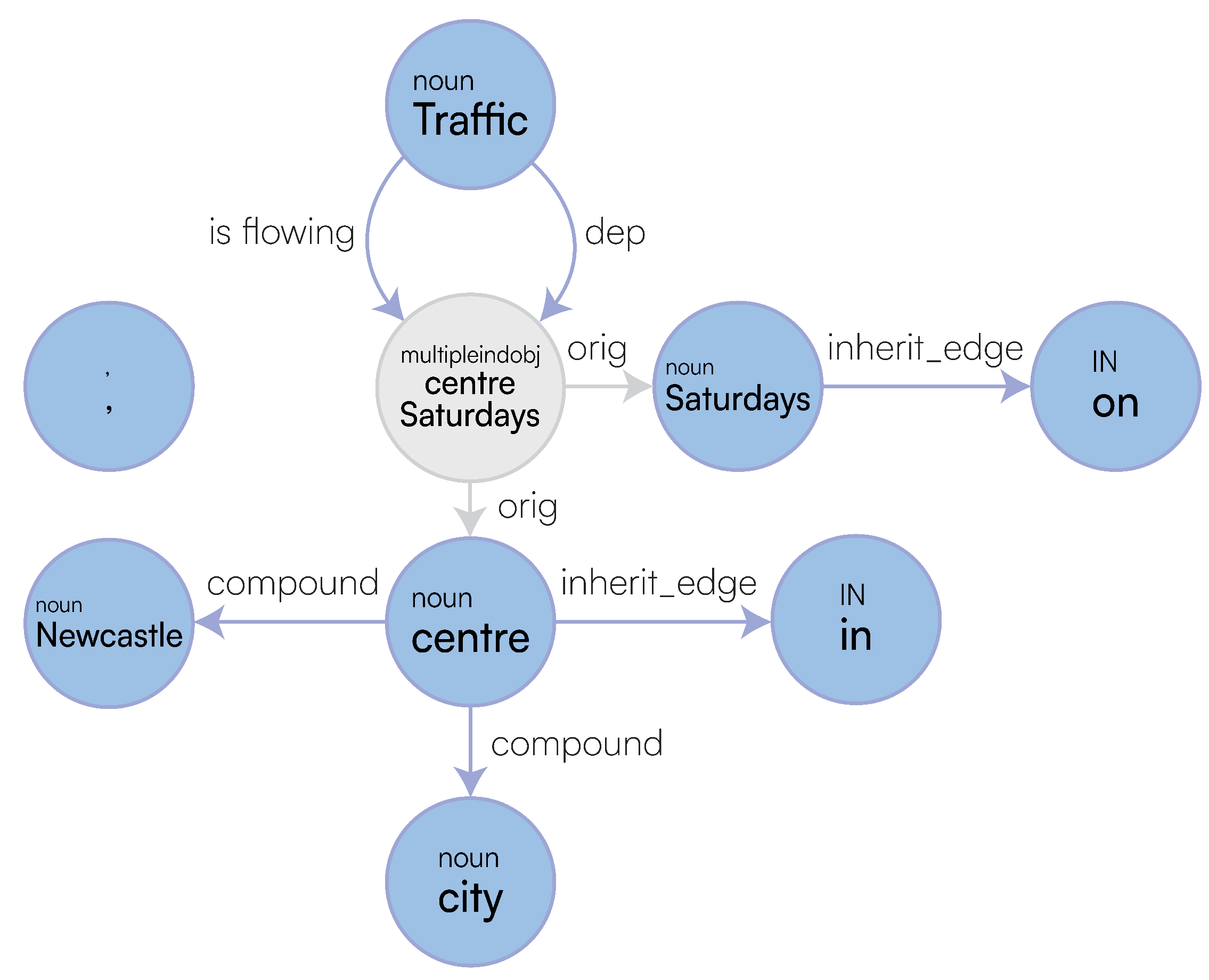
A SetOfSingletons is a specific type of Singleton containing multiple entities, which is an array of Singletons. Such group of items is generated by coalescing distinct entities grouped into clusters as indicated by ud relationships, such as coordination of several other entities or sentences (conj), the identification of multi-word entities (compound), or the identification of multiple logical functions attributed to the same sentence (multipleindobj, derived after GGG rewriting of the original ud graph). Each SetOfSingletons can be associated with type information.
Last, compound_prt relationships: differently from the above, are coalesced into one Singleton as they represent a compound word: ( s h u t ) c o m p o u n d _ p r t ( d o w n ) becomes ( s h u t d o w n ) .

Coordination

For coordination induced by conj relationships, we can derive a coordination type to be AND, NEITHER, OR. This is derived through an additional cc relationship on any given node through a Breadth-First Search (BFS) that will determine the type.

Multi-Word Entities

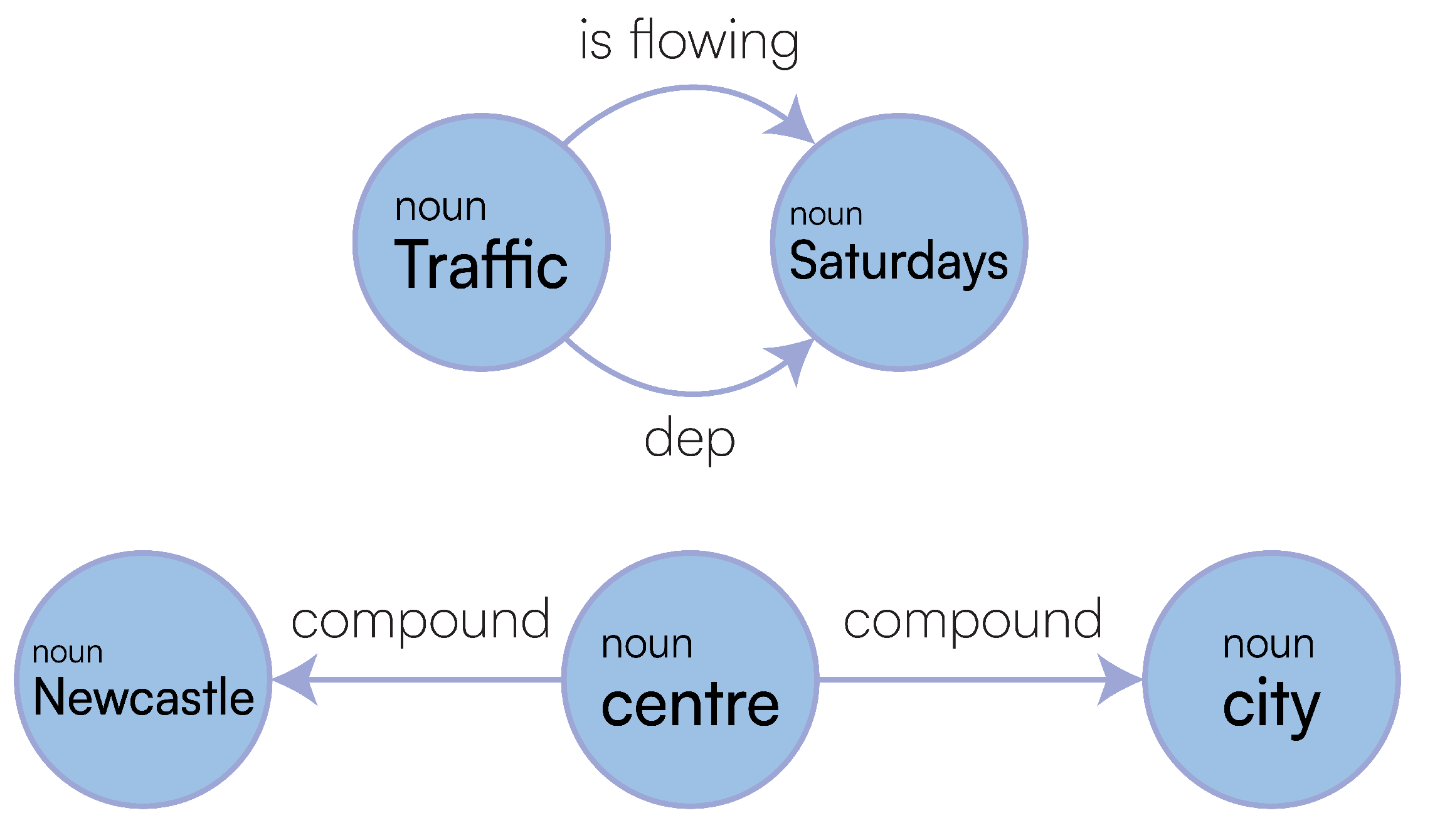
Compound types are simply labelled as a type GROUPING. There are two scenarios where compound edges present themselves, first in a chain, ( a ) c o m p o u n d ( b ) c o m p o u n d ( c ) , or second, a parent node has multiple children directly descending from it, ( b ) c o m p o u n d ( a ) c o m p o u n d ( c ) (Newcastle city centre from Figure 4). To detect these structures, we use the Depth-First Search (DFS) as entities that may have children that present extra information to their parents that should be identified before the resolution of the parents. In the pipeline, these edges are removed, with the children either appended to the parent node’s name, or added as an extra property of the parent, as aforementioned. These can be further refined to separate the main entity from any associated specification (Section 3.2.3).
Example 1.
Looking at the second case, we can focus on “Newcastle city centre”, which has edges ( city ) c o m p o u n d ( centre ) c o m p o u n d ( Newcastle ) . Here,Newcastlecrucially needs to be resolved, to identify it is aGeoPolitical Entity (GPE)for when we merge all the Singletons, within Algorithm 1.

Multiple Logical Functions

As each sentence is represented as a graph, each relationship is binary, meaning we cannot represent n-ary relationships inherently. Therefore, we resort to implementing a SetOfSingletons with a MULTIINDIRECT type as derived from a graph node with multipleindobj label, thus summarising multiple binary relationships. The motivation behind this is clustering all the multiple logical functions into one single node, where orig relationships refer to the original constituents, to ensure the correctness of the graph grammar rewriting. This information is then reified into binary relationships, paving the way for a subsequent logical representation.
Figure 4 has just one sentence with “is flowing” as a verb, where multiple logical functions have as entry points the nodes “centre” and “Saturdays” as ancestors. The node centre Saturdays would become a SetOfSingletons with entities: Newcastle and Saturdays. As we have a node with compound edges within Figure 4, these are resolved into one Singleton: Newcastle[extra:city centre], as per Example 1. Finally, we create our new logical relationships: is flowing(traffic, Newcastle[extra:city centre]) and dep(traffic, Newcastle[extra:city centre]).

3.2.3. Handling Extras

When dealing with multi-word entities, we must identify whether a subset of these words acts as a specification (extra) to the primary entity of interest or whether it should be treated as a single entity. For example, “Newcastle upon Tyne” would be represented as one Singleton with no extra property, whereas “Newcastle city centre” has the core entity being “Newcastle” and an extra being “city centre”.
Algorithm 1: Merge SetOfSingletons
Preprints 154365 i001
To derive which part of the multi-named entity provides a specification for the main entity, we use Algorithm 1: the input takes node, which is the SetOfSingletons to be resolved, and the meu_db referring to the specific sentence of interest. The entities from the given SetOfSingletons is first sorted by the position of each node occurring within the full-text, and a list of alternative representations is created from the power set of its associated entities from which Singletons and empty sets are removed. For example, given an array of three elements: [ x , y , z ] , our layed_alternatives from Line 5 are: [ [ x , y ] , [ y , z ] , [ x , y , z ] ] .
Example 2
(Example 1 cont.). For “Newcastle city centre”, we would be returned with: [ [ Newcastle , city ] , [ city , centre ] , [ Newcastle , city , centre ] ] , representing all the possible combinations of each givenSingletonwithin theSetOfSingletonsto extract theextrafrom the main entity.
We based our inference on a type hierarchy to differentiate between the components providing the specification (extra) to the main entity. The hierarchy of types seen in use on Line 9, employs a Most Specific Type (MST) function to return a Specific Type (ST) from a curated entity-type hierarchy as follows: VERB  < : GPE < : LOC(ation) < : ORG < : NOUN < : ENTITY < :  ADJECTIVE, and if none of these are met, the type is set to None. This is updated from our previous pipeline so that VERB is now the most specific type. Adjectives are also captured, as these were missing from the previous hierarchy.
Last, we look through the meuDB, comparing the minimum and maximum values of the given alternative for a corresponding match which has the highest confidence value (Line 10). These confidence scores lead to how we calculate which alternative should be used for resolving later into our Singleton (Line 12). We check for whether the current candidate in the loop has a greater confidence score than the total confidence score, which is calculated from the product of all confidence scores within the entities.
Example 3
(Example 2 cont.). For our example, we match “Newcastle city”, “city centre”, and “Newcastle city centre”. Given these alternatives, “Newcastle city centre” returns 0.8 (per Section 3.2.1) and “city centre” returns the greatest confidence of 1.0, so our chosen alternative seen at Line 13 is [city,centre]. As “Newcastle” precedes this layer within the sentence, this is selected as ourchosen_entityon Line 36, and subsequently “city centre” becomes theextraproperty to be added to “Newcastle”, resulting in our finalSingleton: Newcastle[extra:city centre].

3.3. Ad Hoc Explanation

While the previous phase dealt with extracting low-level information for all the words contained within the text to provide some preliminary semantic grouping for these, the forthcoming phase provides a gradual ascent of the data representation ladder through which raw full-text data is represented as logical programs, thus achieving the most expressive representation of the text. As this provides an algorithm to extract a specification out of each sentence providing both a human and machine-interpretable representation, we refer to this phase as an ad hoc explanation phase, where information is “mined” structurally and semantically from the text.
The transformation function, τ , takes our full-text enriched with semantic information from the previous phase and rewrites into a final suitable format from which a semantic similarity metric can be used: either a vector-based cosine similarity, a traditional graph-based similarity metric where both node and edge similarity is given through vector-based similarity, potentially capturing the logical connectives represented within each node, or our proposed support-based metric requiring a logical representation for the sentences. Those are then accounting for a different transformation function τ : when considering classical vector-based transformers, we consider the ones available through the HuggingFace library. For our proposed logical approach, the full-text must be transformed as we need a representation that the system can understand to calculate an accurate similarity value produced from only relevant information.
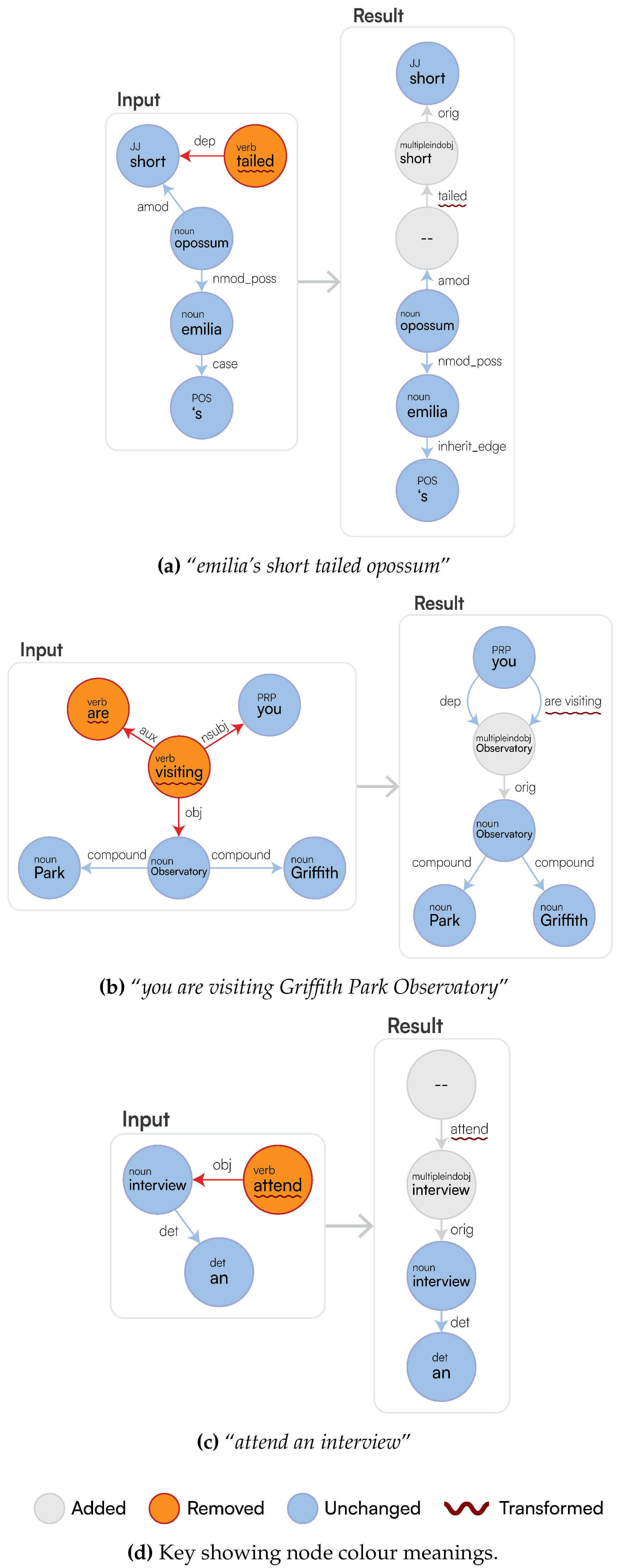
To obtain this, we have distinct subsequent rewriting phases, where more contextual information is gradually added on top of the original raw information: after generating a semi-structured representation of the full-text by enriching the text with ud (Input in Figure 5a, Section 3.3.1), we apply a preliminary graph rewriting phase where we aim to generate similar graphs for sentences being one: the permutation of the other, or two: by simply differing from the active/passive form (Result in Figure 5a, Section 3.3.2). At this stage, we also derive a cluster of nodes (referred to as SetOfSingletons) that can be used later on to differentiate the main entity to the concept the kernel entity is referring to (Section 3.2.3). After this, we acknowledge the recursive nature of complex sentences by visiting the resulting graph in topological order, thus generating minimal sentences first (kernels), for then merging them into a complex and nested sentence structure (Section 3.3.3). After this phase, we extract each linguistic logical function occurring within each minimal sentence using a rule-based approach exploiting the semantic information associated to each entity as derived from the a priori phase (Section 3.3.4). This then leads to the final logical form of a sentence (Figure 5b, Section 3.3.5).

3.3.1. Initial Graph Construction

This step builds an initial graph representation of the sentence based on the syntactic relationships extracted by Stanford CoreNLP through dependency parsing (Section 2.2). Each word in the sentence is represented as a node in the graph, and the syntactic relationships between words (e.g. ud) are represented as edges connecting these nodes. This graph provides a structured representation of the sentence’s syntactic structure, which is then rewritten as described in the forthcoming subsection. Crucially, this process identifies ud, which are essential for our final logical sentence analysis (Section 3.3.4), as this determines the kernel of our sentence and collects additional information associated with it.

3.3.2. Graph Rewriting with the GSM

This step employs the proposed GSM [42] to refine the initial graph and capture shallow semantic relationships merely acknowledging the syntactic nature of the sentence without accounting for the inner node semantic information. Traditional graph rewriting methods, such as the ones for property graphs [43], are often insufficient for our needs. They struggle with creating entirely new graph structures or require restructuring existing ones. We leverage graph grammars [35] within the GSM framework to overcome these limitations. The GSM rewrites the initial graph, incorporating logical connectives and representing verbs as edges between nodes as showed in Figure 5a; among the other operations, this phase normalises active and passive verbs by always generating one single edge per verb, where the source identifies the entity performing the action described by the edge label and, for transitive verbs, the targets might provide information regarding the entity receiving the action from the agent. This restructuring better reflects the syntactic structure and prepares the graph for the final logical rewriting step. If that does not occur, we either flatten out each SetOfSingleton node into one Singleton node (Simple Graphs), or we only retain the logical connectors and flatten out the rest (Logical Graphs). Thus, all the forthcoming substeps are to be considered as relevant for obtaining only the final logical representation of a sentence (Section 3.3.3, Section 3.3.4, and Section 3.3.5). Given that the scope of our work is on the main semantic pipeline and not on the actual graph rewriting queries which were already analysed in our previous work [35], we refer to the online query for more information on the rewriting being encompassed by our current solution (https://github.com/LogDS/LaSSI/blob/32ff1df2df7d824619f9a84e7ae7d7f6e4842cb0/LaSSI/resources/gsm_query.txt, Accessed on 29 March 2025).

3.3.3. Recursive Relationship Generation

In this phase, we carry out some additional graph rewriting operations, which generate binary relationships representing unary and binary predicates by encompassing semantic information for both edge labels and topological orders of the sentences. While the former are clearly represented as binary relationships having a none target argument and usually refer to intransitive verbs, the latter are usually associated with transitive verbs. Either subjects or targets explicitly missing from the text and not expressed as pronouns are resolved into fresh variables, which will then be bound in the logical rewriting phase into an existential quantifier. Given that this phase also needs to consider semantic information, this rewriting cannot be completely encompassed by any graph grammar or general GQL, and therefore, cannot be encompassed entirely by the former phase. This motivates us to hardcode this phase directly in a programming language rather than flexibly representing this through rewriting rules as any other phase within the pipeline.
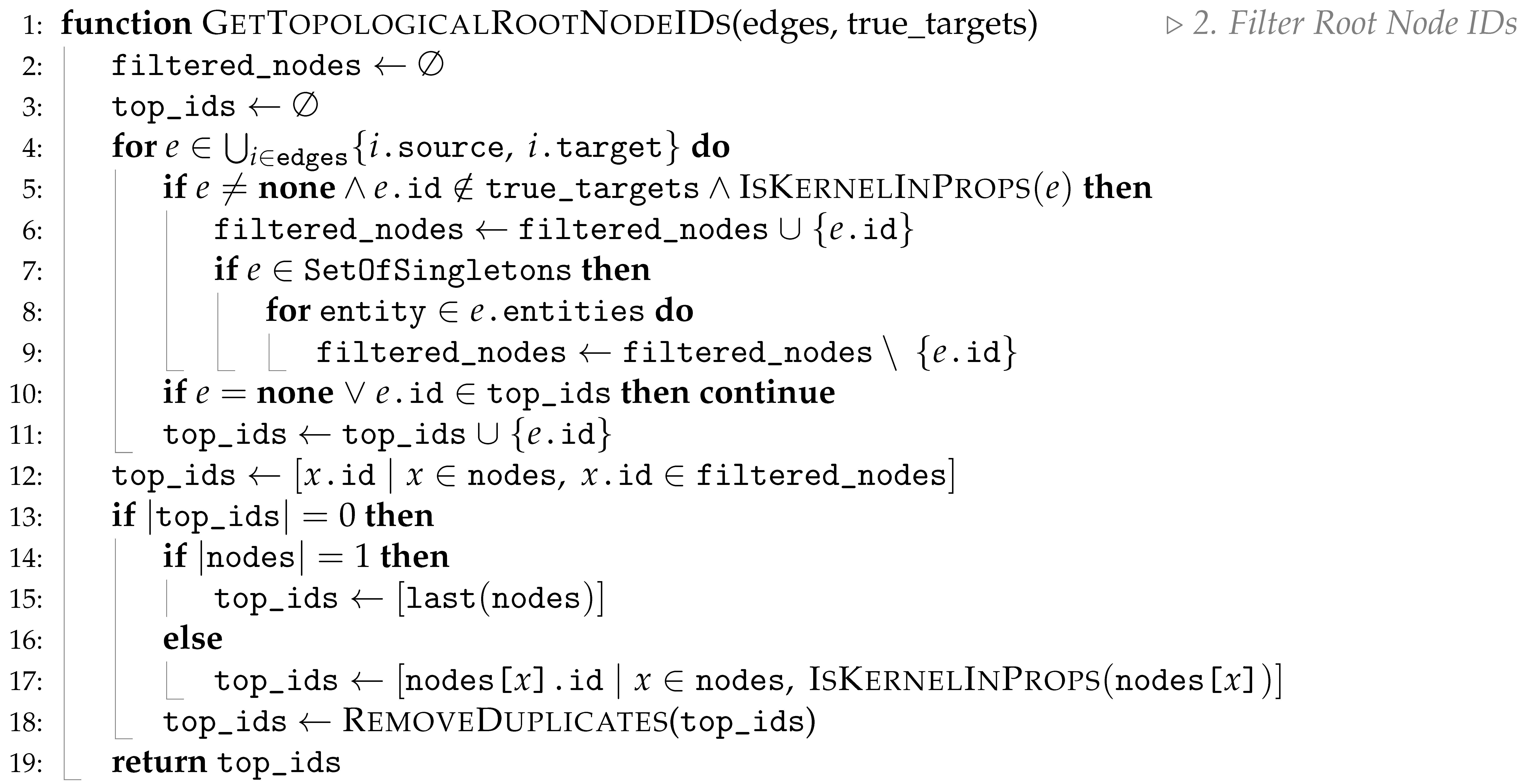
Differently from our previous contribution [16], we now encompass the recursive nature of subordinate clauses [30] by employing a DFS topological sort [44], whereby the deepest nodes in our graph are accounted for first, this can be implemented as every graph is always acyclic; previously, no pre-processing occurred and the graph was read in directly from the rewritten GGG output. The topological sort induces layering on the graph, for which all the siblings of a given node will belong to the same layer; because any operations on the children can be done in any order as they have no dependencies, there are no strict requirements on the order of which the children should appear. We do this to determine which order to apply changes within the graph, by sorting the nodes we minimise the changes by starting from the nodes having the fewer dependencies with the other constituents [35].
Example 4.
Figure 6 demonstrates an example output from DatagramDB, the JSON file generated lists the IDs in the following order: 1, 6, 7, 8, 9, 10, 11, 12, 5, 2, 3. However, once our topological sort is performed, this becomes: 3, 1, 2, 6, 7, 9, 5, 8, 10, 11, 12; our `deepest’ nodes are at the start of our list, and each layer lower follows. A subsequent filtering occurs, which culls nodes from the list that are no longer needed: the edge label between node’s 1 and 3 is inherit_edge, which means all properties of node 3 are added to node 1, and thus node 3 is removed, nodes 12 and 8 contain no information, so can also be removed, and, finally, node 2 (to) has already been inherited into the edge label “to answer ” so is also removed (based on not having any parents or children), resulting in the final sorted list: 1, 6, 7, 9, 5, 10, 11. Our list of nodes within the pipeline is kept in this topological order throughout. Therefore, we can retrieve all roots from the graph to create our kernels.
Unlike the previous simplistic example, most real-world sentences often have a hierarchical structure, where components within the sentence depend on prior elements [35]. Topological sorts then take care of these other more complex situations.
Algorithm 2: Construct Final Kernel
Preprints 154365 i002
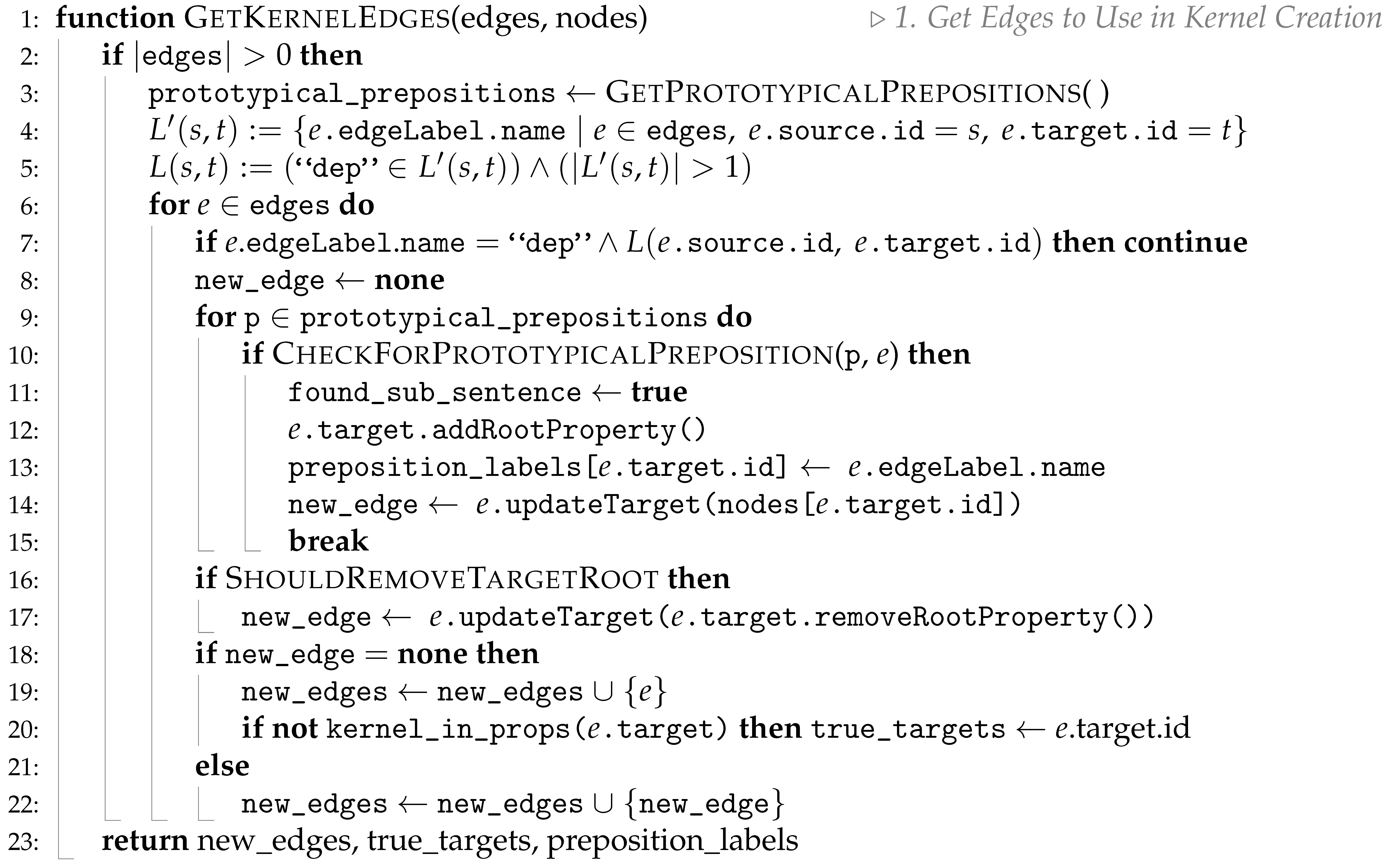
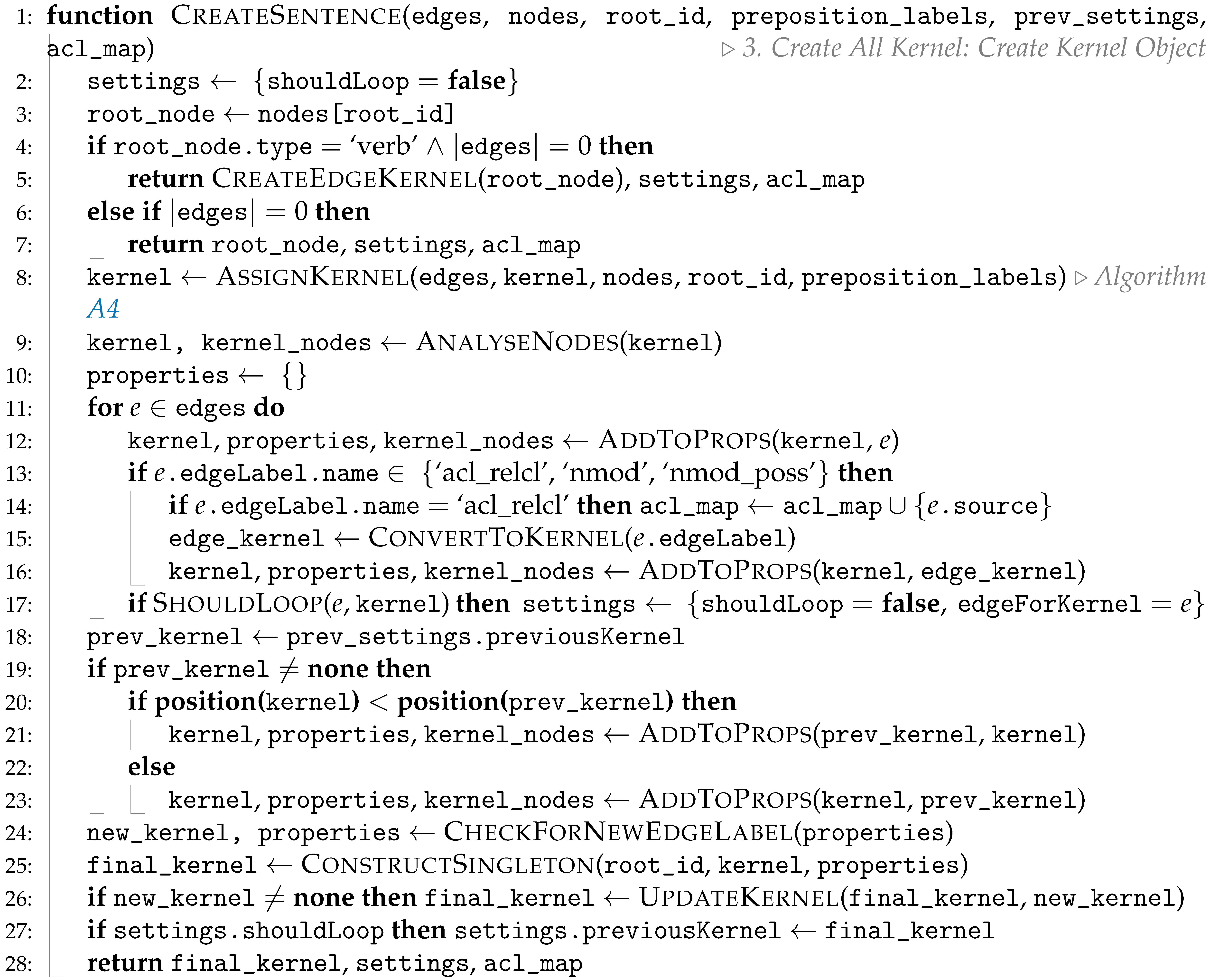
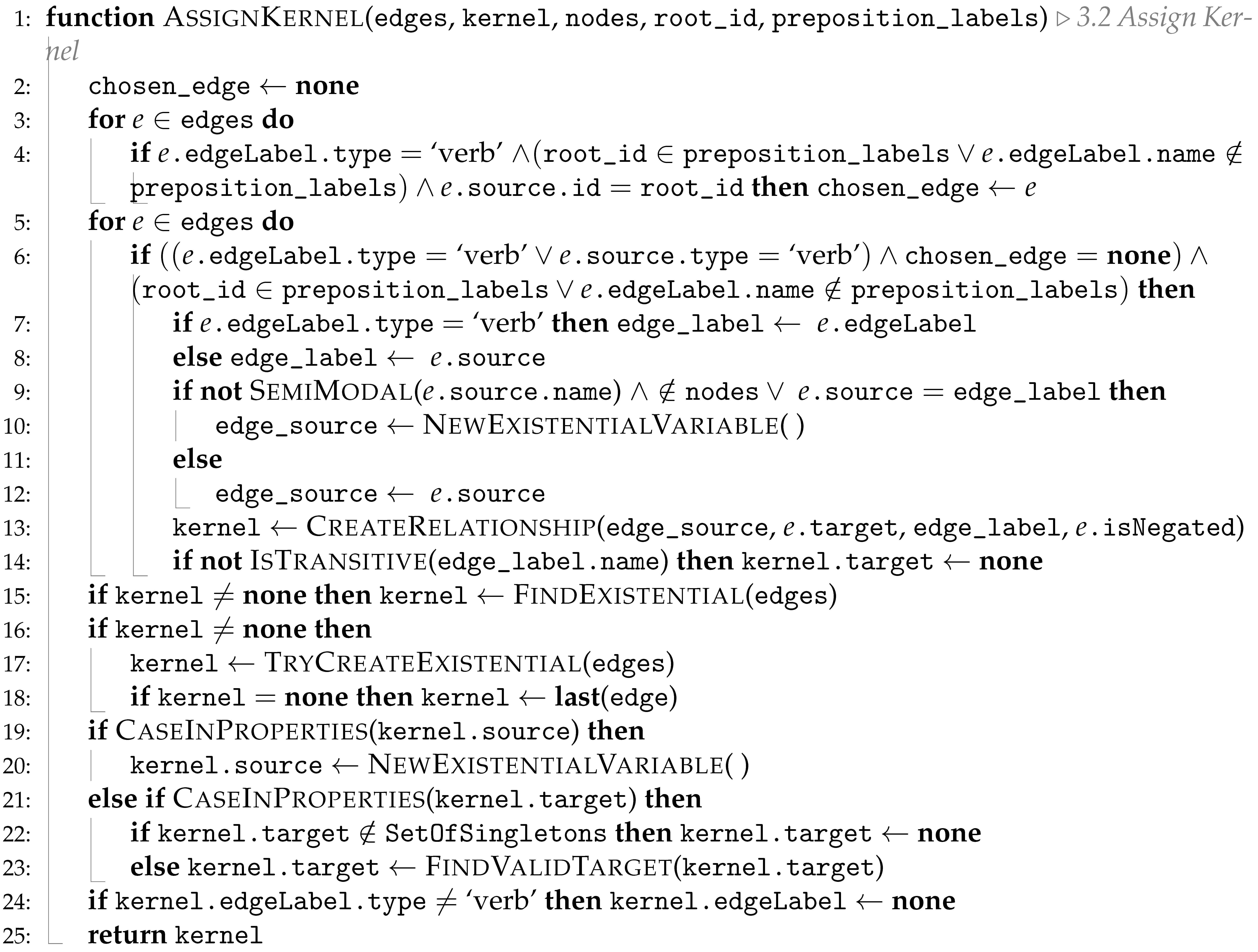
Algorithm 2 sketches the implementation of this phase, where more detailed information is given in Appendix A for conciseness, nesting the different relationships being retrieved through a Singleton. After identifying which edges are the candidates (containing verbs) to become relationships (edges, Line 1), which are the main entry points for each of these to extract a relevant subgraph (top_ids, Line 2), we can now create all relationships representing each verb from the full-text, for then connecting into one single singleton-based tree. After initializing the pre-conditions for the recursive analysis of the sentences (settings on Line 7) for each sentence entry-point to be analysed (n, an ID), we collect all relevant nodes and edges that are associated with it; d all the descendant nodes of n retrieved from a BFS from our new_edges (see Algorithm A1). We then filter the edges by ensuring the following: source and target are contained within the descendant nodes (d) or the target node is in our preposition labels, and the source and target have not already been used in a previous iteration or they have been used in a previous iteration but we have at least one preposition label within the text (Line 10). However, if our loop settings contain a relationship, we use it as our filtered_edges, as we need to create a new one.
CreateSentence only handles rewriting of at most one kernel, whereas another may be contained within the properties of such; therefore, we handle this by returning a possible new kernel through settings.edgeForKernel, and create a new sub-sentence to be rewritten with the same root ID, which is determined from our conditions set out in Appendix A.3. At this stage, we assign our used_edges to our collected filtered_edges for the next (possible) iteration.
After considering only the edges relevant to generate logical information for the sentence and, among those, after electing the relevant one to become a relationship across Singletons as our kernel (Line 13), we further refine the content of the selected edge and perform a post-processing phase (Line 14). If the relationship enclosed in this contains a semi-modal verb [45] in its label, then:
  • If it does have a kernel as a property, and this kernel’s position is contained within our position pairs (collected on Line 5), then we update the target of our kernel to this property as to make an entire kernel describing the action associated to the subject, and introduced by the semi-modal verb.
  • Otherwise, we check if the edge label is none, and whether the source is an adjective and target is an entity, or vice versa. If so, then we update the entity with the properties of the adjective. For example, in the text: “clear your vision”, this is initially rewritten as None(clear, vision) and is transformed to be(vision[JJ: clear], ?), based on this condition.
We also check if we have multiple verbs leading to multiple relationships generating new kernels; if so, we check if this current relationship has no appropriate source or target (Line 16): we refer to these relationships as empty. However, we check within the properties of this kernel to see if a kernel is present within these properties and whether this can be used as our new kernel instead. Following this, we remove all root properties from the nodes used in this iteration to avoid being considered in the next and produce duplicate rewriting. Finally, if we are considering more than one kernel, and the last rewritten kernel is none, then we remove this to ensure that the last successfully rewritten kernel is used for our final kernel. This is selected by taking the ID of the last occurring ID in top_ids, which is the first relationship occurring in topological order for a given full-text (Line 21). Finally, we check if the edge label is a verb; if not, it is replaced with none. Otherwise, we return the kernel.
The final stage of the kernel creation is additional post-processing, to further standardise the final sentence representation (Lines 23-27):
Line 23:
Replaces any occurrence of an acl_relcl edge within the properties, where the source ID is contained within the acl_map, appended to on Line 14 within Algorithm A3, and thus replaced with the node associated in the map. This enables the replacement of any pronoun with the exact entity it is referring to: as our pipeline retains provenance information, this does not come at the cost of losing any information under the circumstance that there are multiple instances of the same entity. We discuss how this has changed from our previous pipeline in Section 5.6.
Line 24:
it checks if we do not have a relationship (where kernel is none) and rewrites this into an edge kernel (Algorithm A3). An edge kernel is where a node of type verb is rewritten to an edge label with no source or target, for example if we had the node `work’ with no other edges, then we return a kernel as such: work(?, None). Otherwise, we deal with verbs that were not rewritten as an edge in our GGG phase and, due to the grammatical structure, were represented as an entity property: action (or actioned) will remark that the entity performs (or receives) the action indicated in action (or actioned). If we have a node with action (or actioned), this entity becomes the source (or target) of the relationship respectively.
Line 25:
Removes duplicated properties occurring in both relationship arguments and their properties: if an entity is contained within the relationship additional properties but is present as either the source or the target of such relationship, then they are removed from properties. This is performed recursively for all kernels.
Line 26:
Rewrites the properties within each kernel as their logical functions. Section 3.3.4 discusses this important phase in more detail.
Line 27:
Last, we deal with phrasal verbs having their adverb separated from the edge relationship name and occurring within the relationship property. If one is found, it is appended to the end of the edge label, which works for some cases, such as `come back’, which is initially come(?[adv:back], None), and therefore becomes come back(?, None), however, it can produce some grammatically incorrect edge label names. For `how to use it’, we get `to use(?[adv:how], it)’, which should have “how” appended to the beginning of the edge label, but currently we get `to use how(?, it)’. This can easily fixed by considering whether the resulting edge belongs to a phrasal verb, and only under that circumstance we can retain such a change.
With all (possible) duplicate properties removed, what remains is logically rewritten based on specific rewriting rules, outlined in the following subsection (Section 3.3.4), after which we can immediately derive the final logical representation of our sentence (Section 3.3.5). This will be the final form for ex post explainability (Section 3.4).

3.3.4. Logical Sentence Analysis

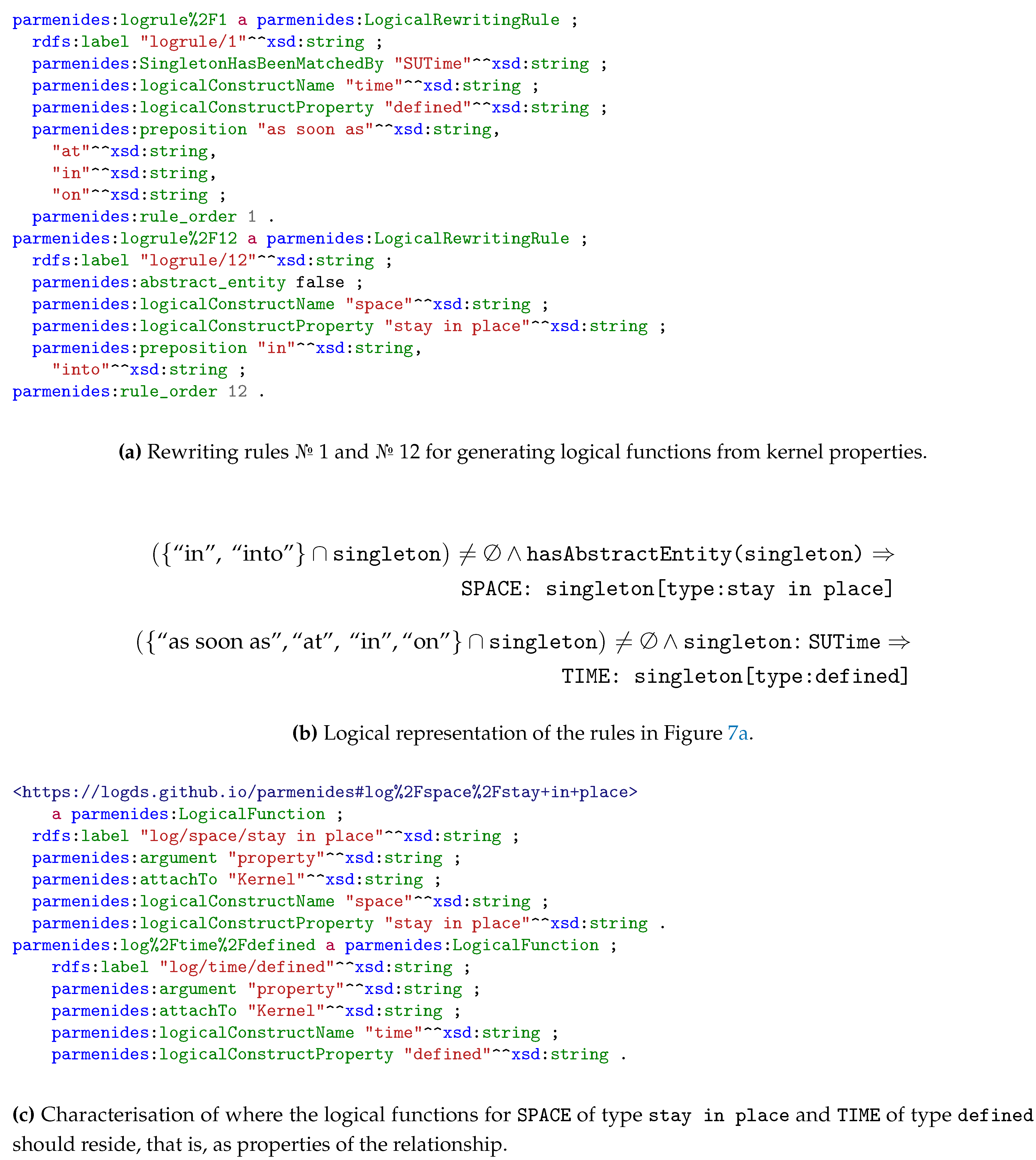
The previous phase provided a preliminary rewriting, where a new relationship is derived from each verb occurring within the pipeline and connecting the agents performing and receiving the action; information concerning additional entities and pronouns occurring within the sentence is collected among the properties associated with the relationship. Given the latter, we now want to rewrite such properties by associating each occurring entity with its logical function within the sentence and recognising any associated adverb or preposition while considering the type of verb and entity of interest. We convey this rewriting mechanism by exploiting simple grammar rules found in any Italian linguistic book (see Section 2.3.1), and therefore easily accessible. To avoid hardcoding these rules in the pipeline, we declaratively represent them as instances of LogicalRewriteRule concepts within our Parmenides ontology (Figure 7a). These rules can be easily defined in Horn clauses (Figure 7b), thus making them easily implementable. Thus, we can then easily extend LaSSI to support further logical functions by extending the rules within the ontology rather than changing the codebase.
Example 5.
Concerning Listing Figure 7a, we are looking for a property that contains a preposition of either “in” or “into”, and is not an entity being an abstract concept. An example sentence that would match this rule is “characters in movies”, before rewriting in Algorithm A5, we get:be(characters, ?)[nmod(characters, movies[2:in])]. Thenmodedge is matched to the rewriting rule, and thus rewritten based on the properties of the matched logical function, presented in Listing Figure 7c, whereby it should be attached to the kernel, resulting in: be(characters, ?6)[(SPACE:movies[(type:stay in place)])].
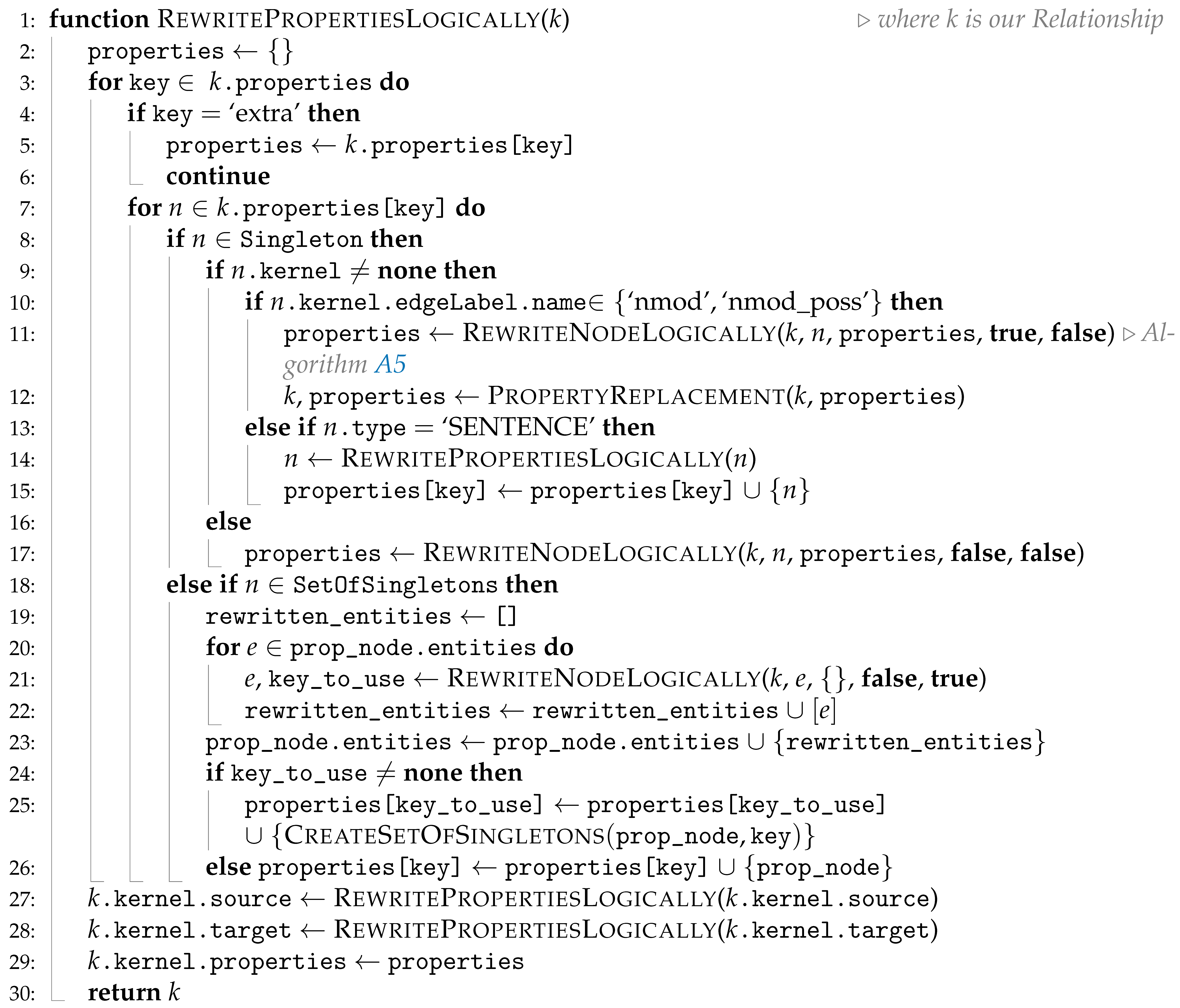
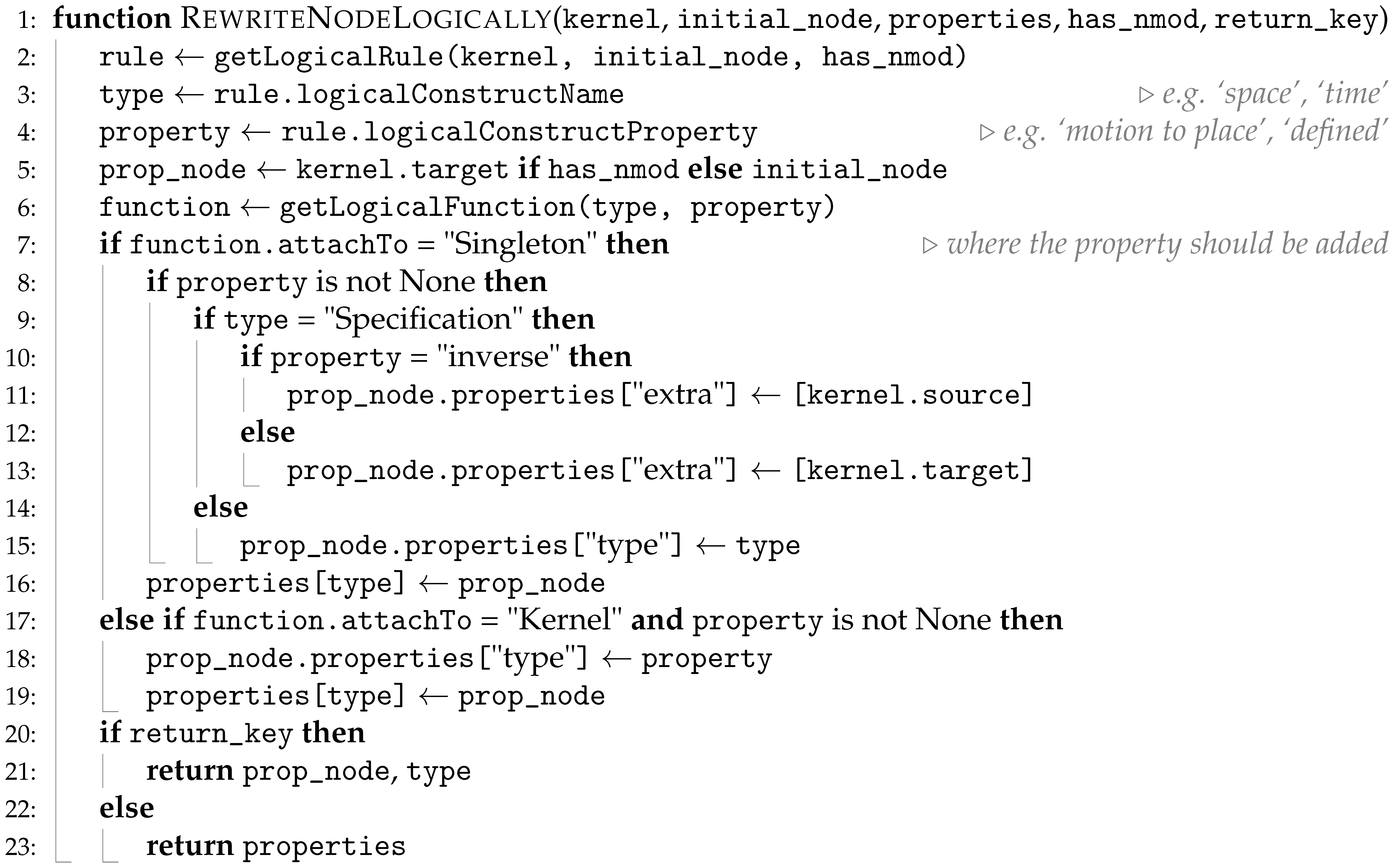
The entailed semantics for the application of these rules is as per Algorithm 3: for each relationship k generated by the previous phase, we select all the Singletons (Line 8) and SetOfSingletons (Line 18) occurring within its properties: for each of the former, we consider them in declaration order (rule order) and, once we found a rule matching some preconditions (premise), we apply the rewriting associated with it and we discard testing for the other rules. When such a condition is met, we establish an association between the logical function determined by the rule and the matched Singleton or SetOfSingletons within the relationship properties. If this is differently stated at the level of the rule, we then move such property to the level of the properties of another Singleton occurring within the relationship of interest (Figure 7c). We perform these recursively for any further nested relationship as part of the properties (Line 17).
Algorithm 3:Logical Properties Rewriting Function
Preprints 154365 i003
Example 6.
`Group of reindeer’ is initially rewritten as:
be(group, ?)[(nmod(group, reindeer[(2:of)]))]
After Line 11 we get:be(group, ?)[SPECIFICATION:group[(extra:reindeer)[2:of]]], which contains some duplication, where we have the source containing group, with properties also of the same entity, but with the additional information of reindeer, therefore, on Line 12, we replace the source with the property and subsequently we get be(group[(extra:reindeer)[2:of]], ?) .
Rule premises may include prepositions from case [46] properties like `of’, `by’, `in’, or predicates based on verbs from nmod [47] relationships, and whether they are causative or movement verbs. There are many different types, like `space’ and `time’, then the property is a further clarification of the type, for `space’ you might have `motion to place’ implying the property has a motion from one place to another, or `stay in place’ implying the location of the sentence is static. For time, we might have `defined’ for `on Saturdays’, or `continuous’, for `during’ implying time for the given sentence is still yet to occur (Table 1).
Example 7.
The sentence “Traffic is flowing in Newcastle city centre, on Saturdays” is initially rewritten as: flow(Traffic, None)[(GPE:Newcastle[(extra:city centre), (4:in)]), (DATE:Saturdays[(9:on)])]: we have both a location of “Newcastle”, and time of “Saturdays”. Given the rules from Figure 7a, the sentence would match the DATE property and GPE. After the application fo the rules, the relationship is rewritten as:
flow(Traffic, None)[(SPACE:Newcastle[(type:stay in place), (extra:city centre)]), (TIME:Saturdays[(type:defined)])]
Due to lemmatisation, the edge label becomes flow from “is flowing”.
For conciseness, additional details for how such a matching mechanism works are moved to Appendix B.

3.3.5. Final FOL Representation

Finally, we derive a logical representation of FOL. Each entity is then represented as one single function, which argument provides the name of the entity, its potential specification value and any adjectives associated with it (cop), as well as any explicit quantification which are pivotal for spatial information from which we can determine if all the parts of the area (all is true) or just some of these (all is false) are considered. This characterisation is not represented as FOL universal or existential quantifiers, as they are only used to refine the intended interpretation of the function representing the spatial entity. Transitive verbs are then always represented with binary propositions, while intransitive verbs are always represented as unary ones; for both, their name refers to the associated verb name. If any ellipsis from the text makes an implicit reference to either of the arguments, these are replaced with a fresh variable, which is then bounded by an existential quantifier. For both functions and propositions, we provide a minor syntax extension which does not substantially affect its semantics, rather than representing a shorthand for avoiding expressing additional function and proposition arguments referring to further logical functions and entities associated with them: we then introduce explicit properties p as key-value multimaps. Among these, we also consider a special constant (or 0-ary function) None, identifying that one argument is missing relevant information. We then derive the following syntax, which can adequately represent factoid sentences as the one addressed in the present paper:
t : T e r m : : = f u n c p ( name , specification , cop , all ) | x V a r
p 1 : P r o p o s i t i o n : : = u p ( t ) | b p ( t , t )
A : F o r m u l a : : = p 1 | ¬ A | A A | A A | x . A
Given the intermediate representation resulting from Section 3.3.3, we then rewrite any logical connective occurring within either the relationships’ properties or within the remaining SetOfSingletons as logical connectives within the FOL representation, and represent each Singleton as a single function. Each free variable in the formula is then bound to a single existential quantifier. When possible, negations potentially associated with specifications of a specific function are then expanded and associated with the proposition containing such function as a term.

3.4. Ex Post Explanation

The ex post explanation phase details the similarity of two full-text sentences through a similarity score over a representation derived from the previous phase. When considering traditional transformer approaches representing sentences as semantic vectors, we consider traditional cosine similarity metrics (Section 3.4.1); when considering graphs representable as a collection of edges, we consider alignment-driven similarities, for which node and edge similarity is defined via the cosine similarity over their full-text representation (Section 3.4.2).

3.4.1. Sentence Embedding

Vector-based similarity systems most commonly use cosine similarity for expressing similarities for vectors expressing semantic notions [48,49], as two almost-parallel vectors will lead to a nearly-1 value, while extremely dissimilar values lead to negative values [50]. This induces the possibility of seeing zero as a threshold boundary for separating similar from dissimilar data. This notion is also applied when vectors represent hierarchical information [51] with some notable exceptions [52]. Given A and B are vector representations (i.e. embedding) from a transformer τ for the sentences α and β , this is S c ( A , B ) = A · B A B . Still, a proper similarity metric should return non-negative values [53]: given the former considerations, we can consider only values above zero as relevant and return zero otherwise, thus having:
S c + ( A , B ) = R e L U ( S c ( A , B ) ) = max { S c ( A , B ) , 0 }
Different transformers generate different vectors, automatically leading to different similarity scores for the same pair of sentences.

3.4.2. Simple Graphs vs. Logical Graphs

Given that our graphs of interest can be expressed as a collection of labelled edges, we reduce our argument to edge matching [12]. Given an edge distance function ϵ , an edge e, and a set of edges A returned from the pipeline as a transformation of the sentence, the best match for e is an edge e A minimising the distance ϵ , i.e. m ϵ ( e , A ) = arg min e A ϵ ( e , e ) . We can then express the best matches of edges in A over another set A as a set of matched edge pairs M ϵ ( A , A ) = { ( e , m ( e , A ) ) | e A } . Then, denote D ϵ ( A , A ) as the set of edges not participating in any match. The matching distance between two edge sets shall then consider both the sum of the distances of the matching edges as well as the number of the unmatched edges [53]. Given an edge-based representation A and B for two sentences α and β generated up until Section 3.3.2, we derive the following edge similarity metric being the basis of any subsequent graph-based matching metric:
S g ϵ ( A , B ) = 1 ϵ ( M ϵ ( A , B ) ) | A | · D ϵ ( A , B ) | N s
Given a node representing a (SetOf)Singleton(s)  ν , an edge label ε , and normalised similarity metric ignoring the negation information, we refine ϵ from Eq. 2 by conjoining the similarity among the edges’ sources and targets, while considering the edge label information. We annihilate such similarity if the negations associated to the edges do not match by multiplying such similarity by 0; then, we negate the result for transforming such similarity into a distance:
ϵ ν , ε ( ( s , t ) , ( s , t ) ) = ν ( s , s ) ν ( t , t ) ε ( λ ( s , t ) , λ ( s , t ) ) neg ( λ ( s , t ) ) = neg ( λ ( s , t ) ) 0 oth .
where ( s , t ) represents an edge and λ ( s , t ) its associated label. This metric can be instantiated in different ways for simplistic and logical graphs by using a suitable definition for ν and ε .

Simple Graphs

For graphs, all SetOfSingletons are flattened to Singletons, thus including the nodes containing information related to logical operators. In these cases we use ν and ϵ as S c + from Eq. (1). At this stage, we still have a symmetric measure.

Logical Graphs

We introduce notation from [53] to guarantee the soundness of the normalisation of distance metrics: we denote d | N = d d + 1 the normalisation of a distance value between 0 and 1, and d | N s = 1 d | N its straightforward conversion to a similarity score.
Now, we extend the definition of ν from Eq. 3 as a similarity ν ( u , v ) : = δ ν ( u , v ) | N s where δ ν is the associated distance function defined in Eq. 4, where we leverage the logical structure of SetOfSingletons; we approximate the confidence metric via an asymmetric node-based distance deriving from fuzzy-logic metrics in combination with matching metrics for score maximisation. We return the maximum distance 1 for all the cases when one logical operator cannot necessarily entail the other.
δ ν ( u , v ) = 1 ν ( u , v ) singleton ( u ) , singleton ( v ) δ ν ( u , m δ ν ( u , v ) ) u i x i , singleton ( v ) 1 δ ν ( x , v ) u ¬ x , singleton ( v ) 1 δ ν ( u , y ) singleton ( u ) , v ¬ y δ ν ( u , m δ ν ( u , v ) ) singleton ( u ) , v i y i δ ν ( x , y ) u = ¬ x , v = ¬ y a v g δ ν ( M δ ν ( u , v ) ) u = i x i , v = i y i , | M δ ν ( u , v ) | = | u | a v g δ ν ( M δ ν ( u , v ) ) u = i x i , v = i y i 1 E δ ν ( u , v ) u = i x i , v = i y i 1 o t h .

3.4.3. Logical Representation

At this stage, we need to derive a logical-driven similarity score to overcome the limitations of current symmetrical measures that cannot capture logical entailment. We can then re-formulate the classical notion of confidence from association rule mining [17] which is implicitly walking in the footsteps of entailment and providing an estimate for conditional probability: from each sentence α and its logical representation A, we need then to derive the set of possible circumstances W ( A ) or worlds in which we trust the sentence will hold. As confidence values are always normalised between 0 and 1, these give us the best metric to represent the degree of trustworthiness of information accurately. We can then rephrase the definition of confidence for logical formulæ  as follows:
Definition 8
(Confidence). Given two logically represented sentences A and B, let W ( A ) and W ( B ) represent the set of possible worlds where A and B hold, respectively. Then, the confidence metric, denoted as confidence ( A , B ) , is defined via its bag semantics as:
confidence ( A , B ) = | W ( A ) W ( B ) | | W ( A ) | W ( A ) 0 o t h .
Please observe that the only formula with an empty set of possible worlds is logically equivalent to the universal falsehood , thus W ( ) ) = .
The forthcoming paragraphs contextualise the way to derive the computation of the formula using our Parmenides ontology and the Closed-World Assumption (CWA) assumption to ensure the correctness of the inference.

Tabular Semantics per Sentence τ ( α ) = A

At this stage, given the impossibility of potentially enumerating all the possible infinite conditions where a specific situation might hold, we focus our interest to the worlds encompassed by the two formulæ  considered within the application of the confidence function. After extracting all the unary U ( A ) or binary B ( B ) propositions occurring within each formula and logical representation A, we can only consider the set of possible worlds circumscribed by the truth or falsehood of each of these propositions. Thus, the set of all the possible worlds where A holds is the set of the worlds where each of the propositions within the formula holds while interpreting each formula using classical semantics [54]. Such semantics is showcased in Example 9.
Example 9.
Consider the sentences α : “Alice plays football” and β : “Bob plays football”. We can represent these logically as binary propositions p 1 : = play(Alice, football)and p 2 : = play(Bob, football), respectively. Given the sentences α: “Alice and Bob play football” and β: “Either Alice or Bob play football”, we can then represent then as A = p 1 p 2 and B = p 1 p 2 where both B ( A ) = B ( B ) = { p 1 , p 2 } . Thus, we can easily derive the set of the possible worlds from the ones arising from all the possible combinations of truth and falsehood of each proposition, as shown in Table 2: Thus, given the corresponding truth table from Table 2, we derive the following values for the bag semantics for A and B: W ( A ) = { # 3 , # 4 } and W ( B ) = { # 2 , # 4 } .
Appendix C.1 formalises the definition of the tabular semantics in terms of relational algebra, thus showcasing the possibility of enumerating all the worlds for which one formula holds while circumscribing them to the propositions that define the formula.

Determining General Implications Through Machine Teaching

As a next step, we want to derive whether each proposition p i B ( A ) U ( A ) occurring in each formula A entails, is equivalent, is indifferent, or is mutually exclusive to another proposition p j B ( B ) U ( B ) in the other formula of interest. As the propositions occurring in the original sentence can be further decomposed into other propositions being either equivalent or logically entailing the former, and given that we want to control that the machine produces sensible and correct rules from the data given, we exploit machine teaching techniques [55,56] to ensure the machine derives correct propositions by exploiting a human-in-the-loop approach [57]. To achieve this, we opt for rule-based semantics [5,15] expanding each distinct proposition p i and p j occurring from the full-text.
Given the inability of Description Logic to represent matching and rewriting statements [58] and given the lack of support flexible properties associated with predicates of current knowledge expansion algorithms which require a fixed schema [5,15], we perform this inference by exploiting an explicit pattern matching and rewriting mechanism. To achieve this, we exploit the Python library FunctionalMatch (https://github.com/LogDS/FunctionalMatch/releases/tag/v1.0, Accessed on 30 March 2025) acting as a derivation mechanism E Γ , K ( p i ) = { p j | K p j } generating propositions p j out of the expansion rules of interest K representing common-sense information and relationship between the entities. We then design the expansion rules Γ and Γ , where the first are used to derive a set of logically entailing propositions E ( p i ) = E Γ , K ( p i ) , while the latter derives a set of equivalent propositions T ( p i ) = E Γ , K ( p i ) .
After this expansion phase, we want to determine whether p i and p j are inconsistent, one entails the other, or whether they are indifferent. At this stage, we define the semantic equivalence p 1 prop p 2 between the expanded propositions via the Parmenides KB, thus deriving a merely semantic correspondence between such propositions. For conciseness, this is narrated in Appendix C.2. This provides a discrete categorisation of the general relationships that might occur between two propositions while remarking whether one entails the other ( ), if they are equivalent ( Eq ), if they are mutually exclusive ( NEq ), or if they are indifferent ( ω ). Differently from our previous paper, we then categorise the previous cases in order of priority as follows:
equivalence:
if p 1 is structurally equivalent to p 2 .
mutual exclusion
:if either p 1 or p 2 is the explicit negation of the other, or whether their negation appear within the expansion of the other ( T ( p 1 ) and E ( p 2 ) respectively).
implication:
if p 1 occurs in one of the expansions E ( p 2 )
If neither of the former conditions hold, we then start the comparison between the T ( p 1 ) and the E ( p 2 ) expanded propositions: given ς the function prioritising the comparison outcomes over a set of compared values (Eq. A4 in the appendix above), we return the comparison outcome as ς ( { p prop q | p T ( p 1 ) , q E ( p 2 ) } ) . After this, we associate with each pair of propositions a relational table from Figure 8, from which we select only the possible worlds of interest where it is plausible to find the worlds occurring.
By natural-joining all the derived tables together into T , thus including the tabular semantics associated with each formula A and B, we trivially reason paraconsistently by only considering the worlds that do not contain contradicting assumptions [59]. We express confidence from Eq. 5 as follows:
support ( s , t ) = a v g π t ( σ s = 1 ( T ) )
While the metric summarises the logic-based sentence relatedness, σ s = 1 ( T ) provides the full possible-world explanation for the number being derived.
Example 10.
From Table 2 and concerning Example 9, we can use these values to determine the confidence value when s t and t s . In our scenario, the resulting equi-join T matches the one from Table 2, as all the propositions are mutually indifferent.
To first find s t ; we find W ( s ) W ( t ) , the number of times s and t are true, which is 1 when both a and b are true. Then, W ( s ) , the number of times s is true, which is also 1, when both a and b are true. Substituting into the confidence metric, we get 1 1 = 100 % , meaning that when a is true, it is certain that b is also true; as when Alice and Bob are playing football, it therefore must hold that either are playing.
Alternatively, to find out t s ; we find W ( t ) W ( s ) , which is 1, the same when both a and b are true. Then, W ( t ) , the number of times t is true, which is 3, when either a or b are true. Substituting into the confidence metric, we get 1 3 = 33 . 3 ˙ % , meaning that when b is true, there is only a 33 . 3 ˙ % chance that a is true; as when either Alice or Bob play football, it cannot be certain that both are playing.

4. Results

The result section is structured as follows: after showing the impossibility of deriving the notion of logical entailment via any symmetric similarity function (Section 4.1), we provide empirical benchmarks showing the impossibility of achieving this through classical transformer-based approaches (Section 4.2). We base our argument on the following observation: given that current symmetric metrics are better suited to capture sentence similarity through clustering due to their predisposition of representing equivalence rather than entailment, we show that assuming symmetrical metrics also leads to incorrect clustering outcomes, out of which dissimilar or non-equivalent sentences are grouped. Experiments further motivate the inability of such transformer-based approaches to adequately distinguish the role of the same entities occurring within the sentence when different sentence forms and negations are given (Section 4.2.2), the inability to capture the nuances offered by logical connectives (possibly due to the interpretation of these as stop words to be removed, Section 4.2.1), and the impossibility of performing spatiotemporal reasoning due to the inability of conveying reasoning mechanisms by force of just semantic similarity (Section 4.2.3). Last, we address the scalability of our proposed approach by considering a sub-sent of full-text sentences appearing as nodes for the ConceptNet common-sense knowledge graph (Section 4.3). Last, the discussion Section (Section 5) provides some reflection on our work and how this improved over our previous version of the LaSSI pipeline.
The experiments were run on a Linux Desktop machine with the following specifications: CPU: 12th Gen Intel i9-12900 (24) @ 5GHz, Memory: 32GB DDR5. The raw data for the results, including confusion matrices and generated final logical representations, can be found on OSF.io (https://osf.io/g5k9q/, Accessed 28 March 2025).

4.1. Theoretical Results

As the notion of verified AI incentivises inheriting logical-driven notions for ensuring the correctness of the algorithms [19], we then leverage the logical notion of soundness [60] to map the common-sense interpretation of a full-text into a machine-readable representation (let that be a logical rule or a vector embedding); a rewriting process is sound if the rewritten representation logically follows from the original sentence, which then follows the notion of correctness. For the sake of the current paper, we limit our interest to capturing logical entailment as generally intended from two sentences. Hence, we are interested in the following definition of soundness:
Definition 11.
Weak Soundness, in the context of sentence rewriting, refers to the preservation of the original semantic meaning of the logical implication of two sentences α and β. Formally:
Weak Soundness : if S α β , then also φ τ ( α , β )
where S is the common-sense interpretation of the sentence, ⊑ is the notion of logical entailment between textual concepts, and φ τ is a predicate deriving the notion of entailment from the τ transformation of a sentence via the choice of a preferred similarity metric S .
In the context of the paper, we are then interested in capturing sentence dissimilarities in a non-symmetrical way, thus capturing the notion of logical entailment:
Correctness : α β β ¬ α φ τ ( α , β ) ¬ φ τ ( β , α ) .
The following results remark that any symmetric similarity metrics (thus including the cosine similarity and the edge-based graph alignment) cannot be used to express logical entailment (Section 4.1.1), while the notion of confidence adequately captures the notion of logical implication by design (Section 4.1.2). All the proofs for the forthcoming lemmas are moved to Appendix D.

4.1.1. Cosine Similarity

This entails that we can always derive a threshold value θ above which we can deem as one sentence implying the other, thus enabling the following definition:
Definition 12.
Given α and β are full-text and τ is the vector embedding of the full-text, we derive entailment from any similarity metric S as follows:
φ τ ( α , β ) θ . S ( τ ( α ) , τ ( β ) ) > θ ,
where θ is a constant threshold. This definition allows us to express implications as exceeding a similarity threshold.
As cosine similarity captures the notion of similarity, and henceforth an approximation of a notion of equivalence, we can clearly see that such metric is symmetric.
Lemma 13.
Cosine similarity is symmetric
Symmetry breaks the capturing of directionality for logical implication. Symmetric similarity metrics can lead to situations where soundness is violated. For instance, if A B holds based on a symmetric metric, then B A would also hold, even if it’s not logically valid. We derive implication from similarity when the similarity metric for A B is different to B A , given that A ¬ B , and this shows that one thing might imply the other but not vice versa. To enable the identification of implication across different similarity functions, we entail the notion of implication via the similarity value as follows:
Lemma 14.
All symmetric metrics S trivialise logical implication:
S s y m m φ τ ( α , β ) φ τ ( β , α )
Since symmetric metrics like cosine similarity cannot capture the directionality of implication, they cannot fully represent logical entailment. This limitation highlights the need for alternative approaches to model implication accurately, thus violating our intended notion of correctness.

4.1.2. Confidence Metrics

Differently from the former, we show that the confidence metric presented on Section 3.4 produce a value that aims to express logical entailment under the assumption that the φ transformation from full-text to logical representation is correct.
Lemma 15.
When two sentences are equivalent, then they always have the same confidence.
A B confidence ( A , B ) = confidence ( B , A ) = 1
As a corollary of the former, this shows that our confidence metric is non-symmetric.
Corollary 16.
Confidence provides an adequate characterisation of logical implication.
¬ ( A B ) confidence ( A , B ) < 1
This observation leads to the definition of the following notion of φ τ given τ the processing pipeline:
Definition 17.
Given α and β are full-text and τ is the logical representation of the full-text as derived from the ad hoc phase (Section 3.3), we derive entailment from any similarity metric S as follows:
φ τ ( α , β ) confidence ( τ ( α ) , τ ( β ) ) = 1

4.2. Clustering

While the previous section provided the basis for demonstrating the theoretical impossibility of achieving a perfect notion of implication, the following experiments are aimed at testing this argument from a different perspective: we want to test which of these metrics is well-suited for expressing the notion of logical equivalence as per original design. Given that the training-based approach cannot ensure a perfect notion of equivalence returning a perfect 1 score for extremely similar sentences, we can relax the argument by requiring that there exists any suitable clustering algorithm allowing to group some sentences of choice by distance values providing the closest match to the group of expected equivalent sentences of choice. Then, the correctness of the returned clustering match is computed using a well-defined set-based alignment metric from [53] being a refinement of Eq. 2 using ϵ ( s , t ) = 1 s = t , where 1 P is the indicator function returning 1 if and only if (iff). the condition P holds and 0 otherwise [61]. To remove any semantic ambiguity derivable from analysing complex sentences with multiple entities, we consider smaller ones so to have controlled experiments under different scenarios: distinguishing between active and passive sentences (Figure 12a), considering logical connectives within sentences (Figure 10a), and expressing simple spatiotemporal reasoning (Figure 13a). If, under these considerations, the current state-of-the-art textual embeddings cannot capture the notion of sentence similarity by always returning clusters not adequately matching the expected ones (Figure 12b, Figure 10b and Figure 13b), we then could then conclude that these representations are not well-suited to capture reasoning-driven processes, thus corroborating the observations from preliminary theoretical results [62].

Deriving Distance Matrices from our Similarity Metrics and Sentences

We use transformers τ as made available via HuggingFace [63] coming from the current state-of-the-art research papers:
  • all-MiniLM-L6-v2 [64]
  • all-MiniLM-L12-v2 [64]
  • all-mpnet-base-v2 [65]
  • all-roberta-large-v1 [66]
For all the approaches, we consider all similarity metrics s ( A , B ) already being normalised between 0 and 1 as discussed in Section 3.4. We can derive a distance function from this by subtracting such value by one, hence d ( A , B ) : = 1 s ( A , B ) . As not all of these approaches lead to symmetric distance functions and given that the clustering algorithms work under symmetric distance functions, we obtain a symmetric definition by averaging the distance values as follows:
d ¯ ( a , b ) : = 1 2 ( d ( a , b ) + d ( b , a ) )

Clustering Algorithms of Choice

We test our hypothesis over two clustering algorithms supporting distance metrics as an input rather than a collection of points in the d-dimensional Euclidean space, Hierarchical Agglomerative Clustering (HAC) and k-Medoids.
HAC [67] is a hierarchical clustering method that uses a `bottom-up’ approach, starting with creating the clusters from the data points having the least distance. By considering each data point as a separate cluster, these are iteratively merging the least distance pair of clusters according to a given linkage criterion until we reach the number of the desired clusters, by which point the clustering algorithm will stop [68]. The graphs visualised in Figure 9, Figure 11, and Figure 14 are dendograms, which allow for exploring relationships between clusters at different levels of granularity. In our experiments, we consider the complete link criterion for which the distance between two clusters is defined as the distance between two points, each for one single cluster, maximising the overall distance [69].
k-Medoids [70] is a variation of the k-Means Clustering where, as a first step, the algorithm will start by picking actual data points as centres of the cluster while being suited to support distance metrics by design. Assuming these initial medoids as centres of their clusters, each point is assigned to the cluster identified by the nearest medoid. At each step, we might consider swapping a medoid with another node if this minimises the clustering assignment costs. The iteration converges after a maximum number of steps or when we reach stability, i.e., no further clusters are updated. As this approach also minimises a sum of pairwise dissimilarities rather of a sum of squared Euclidean distances as k-Means, k-Medoids is more robust to noise and outliers than k-Means.
Figure 9. Dendogram clustering for ’Alice and Bob’ sentences.
Preprints 154365 g009
We consider the k-Medoids algorithm with an initialisation being a variant of k-means++ [71] considering the initial k-Medoids for the clusters for avoiding bad initialisations resulting by selecting initial random points by otherwise sampling these initial points over “an empirical probability distribution of the points’ contribution to the overall inertia” (https://scikit-learn.org/stable/modules/generated/sklearn.cluster.KMeans.html, Accessed on 29 March 2025). No further hyperparameter tuning is required under these assumptions, as these annihilate the need for doing multiple tests with multiple different random seeds. We consider the implementation of HAC from scikit-learn v1.6.0 (https://scikit-learn.org/stable/whats_new/v1.6.html#version-1-6-0, Accessed on 29 March 2025) and, given that this library does not implement k-Medoids, we use scikit-learn-extra v0.3.0 (https://scikit-learn-extra.readthedocs.io/en/stable/changelog.html#unreleased, Accessed on 29 March 2025).

4.2.1. Capturing Logical Connectives and Reasoning

We want to prove that state-of-the-art vector-based semantics from the sentence transformers cannot represent logical connectives appearing in sentences, thus postulating the need for explicit graph operators to recognise the logical structure of sentences. We are also checking if the logical connectives are also treated as stop words by transformers, thus being ignored. This is demonstrated through sentences in Figure 10a, whereby one sentence might imply another, but not vice versa. However, with our clustering approaches, we only want to cluster sentences that are similar in both directions, therefore our clusters remain as only having one element, as shown in Figure 10.
Figure 10. Sentences and expected clusters for `Alice and Bob’.
Preprints 154365 g010
Analysing Table 3, all approaches perfectly align with the expected clusters. However, this is determined by the nature of HAC, since the algorithm starts with this exact configuration where each element it its own cluster, it inherently matches the ground truth from the beginning; therefore, before any merging even occurs, the algorithm has already achieved perfect alignment.
Instead, investigating the graphs in Figure 9, we can see that for our Simple Graphs in Figure 9a, this approach fails to recognise directionality and does not produce appropriate clusters, even failing to recognise similarity a sentence has with itself. Logical Graphs shown in Figure 9b improve, recognising similarity for 2 ⇒ 0 for example, however, producing a similarity of 0 for 0 ⇒ 2. Finally, our Logical representation in Figure 9c successfully identifies directionality and appropriately groups sentences together. For example, 2 ⇒ 0 is entirely similar, however, 0 ⇒ 2 is only slightly similar, which entails as “Alice and Bob play football” implies that “Alice plays football”, but it does not necessarily hold that both Alice and Bob play football if we only know that Alice plays football.
The sentence transformer approaches displayed in Figure 9d–g all produce similar clustering, with high similarities between sentences in the dataset that are incorrect; for example clustering Alice does and does not play football are closely related according to the transformers, as aforementioned, this is most likely due to the transformers use of edit-distance, therefore not capturing a proper understanding of the sentences, whereas our approach does, by showing they are dissimilar.
Figure 11. Dendogram clustering for ’Cat and Mouse’ sentences.
Preprints 154365 g011

4.2.2. Capturing Simple Semantics and Sentence Structure

The sentences in Figure 12a are all variations of the same subjects (a cat and mouse), with different actions and active/passive relationships. The dataset is set up this way to produce sentences with similar words but in a different order to tackle whether sentence embedding understands context from structure rather than edit distance. Figure 12b shows the expected clusters for the `Cat and Mouse’ dataset. 0 and 1 are clustered together because the action from the subject on the direct object is the same in both: `the cat eats the mouse’ is equivalent to `the mouse being eaten by the cat’. Similarly, sentences 2 and 3 are the same, but with the action reversed, the mouse eats the cat in both.
Figure 12. Sentences and expected clusters for `Cat and Mouse’.
Preprints 154365 g012
Analysing Table 4, we can see that all stages of the LaSSI pipeline achieve perfect alignment with HAC and k-Medoids, effectively capturing the logical equivalence between sentences 0 and 1, and 2 and 3. We can see a gradual increase in the matched clusters in Figure 11a, Figure 11b, and Figure 11b, as the contextual information within the final representation increases with each different sentence representation. Each representation shows a further refinement within the pipeline. The clustering shows values are near to each other, thanks to structural semantics, but does not determine that they are the same. The first two approaches (Simple and Logical Graphs) roughly capture the expected clusters we are looking for but does not encapsulate the entire picture from the similarity of the sentences in the whole dataset, our final logical representation produces the expected perfect matches with {0, 1}, and {2, 3}. This suggests LaSSI can identify the same relationship between the “cat” and “mouse”, despite different syntactic structures via active and passive voice.
All the transformer models show lower alignment with HAC and k-Medoids, 0.3750, implying that while they capture some semantic similarity, they struggle to fully grasp the logical equivalence between the sentences in the same way LaSSI does, and even with some simplistic rewriting from our pipeline, we outperform these state-of-the-art transformers. Figure 11d–g all show much larger clusters from the ones we would expect, grouping together sentences incorrectly. None of these transformers produces zones with 0 similarity, as they determine all the sentences are related to each other, misinterpreting that “The cat eats the mouse” and “The mouse eats the cat” are similar.
The pipeline for these given transformers will ignore stop words which may also impact its resulting scores; we also recognise that the similarity is heavily dominated by the entities occurring, while the sentence structure is almost not reflected: transformers are only considering one sentence as a collection of entities without taking the structure of the sentence into account, whereby changing the order will yield similar results and therefore cannot derive sentence structure. By interpreting similarity with compatibility, graph-based measures exclude entirely the possibility of this happening, while logic-based approaches are agnostic.

4.2.3. Capturing Simple Spatiotemporal Reasoning

We have multiple scenarios involving traffic in Newcastle, presented in Figure 13a, which has been extended from our previous paper to include more permutations of the sentences. This was done so that we have multiple versions of the same sentence that should be treated equally by ensuring the rewriting of each permutation is the same, therefore resulting in 100% similarities.
Figure 13. Sentences and expected clusters for `Newcastle’.
Preprints 154365 g013
Analysing the results in Table 5, we can see that our Logical Graphs and Logical approaches outperform the transformers, with our final logical approach achieving 100% alignment against the expected clusters. Our initial approaches fail to fully capture proper spatiotemporal reasoning of the sentences, essentially only capturing the similarity of sentences with themselves. For Simple Graphs in Figure 14a, we can see some similarity detected between sentences 7 (“Traffic is flowing in Newcastle city centre, on Saturdays”) and 8 (“On Saturdays, traffic is flowing in Newcastle city centre”), which is correct, however it should be treated as having 100% similarity, which it does not here. Furthermore, the majority of the dendrogram shows little similarity across the dataset. We see an increase in overall clustering similarity for both HAC and k-Medoids in the Logical Graphs approach, shown in Figure 14b, now also capturing similarity between a few more sentences, but overall still not performing as expected. Finally, our Logical approach presents an ideal result, with 100% clustering alignment and a dendrogram that presents clusters that fix our expected outcome. {0,1,9} and {6,7,8} are clustered together, as we would expect, and we also see some further implications being presented. Sentences 0, 1, and 9 (All state: there is traffic in the Newcastle city centre) are clustered towards sentence 4 (“It is busy in Newcastle”), presenting that if there is traffic in Newcastle city centre, then Newcastle is busy, however this similarity is only 50% in the other direction, as if it is busy in Newcastle, we cannot know for certain that this is caused by traffic. We also correctly see negation being acknowledged, with sentences 0 (“There is traffic in the Newcastle city centre” and 10 (“Newcastle city center does not have traffic”) for example being treated as having 0% similarity. Furthermore, a complex implication is captured between 2 and 11. Sentence 2 states that “There is traffic but not in the Newcastle city centre”, meaning there is traffic somewhere, but just specifying that it isn’t in Newcastle city centre, while sentence 11 states: “Newcastle has traffic but not in the city centre”, a subtle difference not captured by any other approach presented. Our Logical approach shows complete similarity for 2 ⇒ 11, but a 50% for 11 ⇒ 2, as there being traffic but not in the Newcastle city centre, implies that there is not traffic in the Newcastle city centre, but if we only know there is not traffic in the city centre, then we cannot know there is traffic everywhere else.
Figure 14. Dendogram clustering graphs for ’Newcastle’ sentences.
Preprints 154365 g014
The sentence transformer approaches produce a very high similarity for nearly all sentences in the dataset. There are discrepancies in the returned clusters from what we would expect for several reasons. The word embeddings might be capturing different semantic relationships. For example, “busy” in sentence 4 (“It is busy in Newcastle”) might be considered similar to the “busy city centers” in sentence 5 (“Saturdays have usually busy city centers”), leading to their clustering, even though the context of Newcastle being busy is more general than the usual Saturday busyness. We can see that sentences related to Saturdays (5, 6, 7, 8) form a relatively cohesive cluster in the dendrogram, which aligns with the desired grouping for 6, 7, and 8. However, sentence 5’s early inclusion with the general “busy” statement (4) deviates from the intended separation. Furthermore, the embeddings might be heavily influenced by specific keywords, the presence of “Newcastle city centre” in multiple sentences might lead to their clustering, even if the context around traffic flow or presence is different. As discussed previously, these transformers cannot differentiate between the presence and absence of traffic as intended in the desired clusters. For example, sentence 10 (“Newcastle city center does not have traffic”), is clustered with sentence 2 (“There is traffic but not in the Newcastle city centre”), which is incorrect.

4.3. Sentence Scalability Rewriting

We have broken down the different phases of our LaSSI pipeline and performed scalability experiments with 200 sentences gathered from nodes from ConceptNet [18].
Loading sentences refers to injecting a .yaml file containing all sentences to be transformed into Python strings.
Generating meuDB (Section 3.2.1) takes the longest time to run, as it relies on Stanza to gather POS tagging information for every word in the full text. We also perform fuzzy string matching on the words to get every possible multi-word interpretation of each entity, which increases dramatically as the amount of sentences increases. However, once it has been generated, it is saved to a JSON file, which is then loaded into memory for subsequent executions, represented by the loading meuDB phase.
Generating the gsmDB (Section 3.3.2) uses the learning-based pipeline from StanfordNLP, however still achieves a speedy execution time, with generating our rewritten graphs performs even better, as this is not dependent on any learning-based pipeline.
Generating the intermediate representation (Section 3.3 except from Section 3.3.5) ends up being slower than generating the GSM graphs, which is most likely because the pipeline is being throttled when lemmatising verbs at multiple stages in the pipeline. This is because the pipeline is attempting to lemmatise each single word alone occurring within the text, while the GSM generation via StanfordNLP considers the entire sentences as a whole. We boosted this by using LRU caching mechanism [72,73] from functools, so words that have already been lemmatised can be reused from memory. However, as the number of sentences increase, so does the number of new words. As the other rewriting steps are streamlined through efficient algorithms providing efficient implementations for rule matching and rewriting mechanisms, future works will address better strategies for enhancing the current rewriting step.
Given the plots, all processing steps discussed have a linear time complexity modulo time fluctuations: as all the algorithms used in this paper mainly entail the rewriting of original sentences by reading them from the beginning to the end independently from their representation, the least cost we can pay is comparable to a linear scan of the data representation for each sentence. This then remarks that further improvements over the provided algorithms can be only achieved through decreasing additive and multiplicative constant factors.
At the top end of our tests (highlighted in the red bounding box in Figure 15), it took on average 59.40 minutes for 200 sentences on a single-threaded machine, and once the meuDB was generated it took 8.84 seconds. In comparison, the time taken to train OpenAI’s GPT-3 model took ≈34 days on 1024 GPUs [74]. If this were executed on a single-threaded machine like ours, it would take ≈355 years, proving how advantageous our pipeline is. Therefore, our pipeline is correct and more efficient at deriving expected sentence similarity results.

5. Discussion

We now provide some preliminary results that we carried out by analysing the real-world 200 sentences benchmarked in the last experiment (Section 4.3), while sentences explicitly mentioning Newcastle and traffic scenarios are derived from our Spatiotemporal reasoning dataset (Figure 13a). For the former dataset, we were able to accurately describe in logical format about 80% of the sentences, while still improving over our previous implementation, the differences with which are narrated below.

5.1. Improving Multi-Word Entity Recognition with Specifications

Our previous solution [16] chose the most recently resolved entity and did not account for scenarios where multiple resolutions with equal confidence occur. Algorithm 1 rectifies this: on each possible powerset of the SetOfSingletons entities (Line 5), we check if the current item score is greater than anything previously addressed (Line 12) and, if so, we use this resolution in place of the former. Furthermore, if we have multiple resolutions with the same score, we choose the one with the greatest number of entities (Line 31). For example, the sentence “you are visiting Griffith Park Observatory” contains a SetOfSingletons, with entities: Griffith, Park, and Observatory. Two resolutions with equal confidence scores are resolved, the first being Observatory with an extra: Griffith Park, and the second: Griffith Park Observatory, so based on Line 31, we use the latter as our resolved entity. This is a preliminary measure and could change in future with further testing, but current experiments prove this to be a valid solution.

5.2. Using Short Sentences

We have restricted our current analysis to full-text with no given structure, as in ConceptNet [18], instead of being parsed as semantic graphs. These can be represented in propositional logic, in which no universal quantifiers are given, only existential. If we cannot capture propositional logic from these full-texts, then we cannot carry out FOL as the latter is a more expressive logical fragment of the former. In propositional logic, the truth value of a complex sentence depends on the truth values of its simpler components (i.e. propositions) and the connectives that join them. Therefore, using short sentences in logical rewriting is essential because their validity directly influences the validity of larger, more complex sentences constructed from them. If the short sentences are logically sound, the resulting rewritten sentences will also be logically sound and we can ensure that each component of the rewritten sentence is a well formed formula, thereby maintaining logical consistency throughout the process. For example, consider the sentence “It is busy in Newcastle city centre because there is traffic” This sentence can be broken down into two short sentences: “It is busy in Newcastle city centre” and “There is traffic”. These short sentences can be represented as propositions, such as P and Q. The original sentence can then be expressed as Q P . By using short sentences, we ensure that the overall sentence adheres to the rules of propositional logic [75].

5.3. Handling Incorrect Verbs

We cannot rely on StanfordNLP’s dependency parsing, as it can fail to distinguish the proper interpretation of a sentence [76], severely impacting our representation when verbs are incorrectly identified.
In Figure 16a, “short” and “tailed” should both be identified as amod’s of opossum, however we instead get “tailed” as a verb, rewritten as an edge towards the adjective short. Therefore, given this interpretation, LaSSI rewrites the sentence to: be( opossum emilia s , ?)[SENTENCE:tail( ? cop : short , None)]. We can see that because of “tailed” being identified as a verb, a kernel is created which is incorrect. However, given the interpretation from the parser, this is the best rewriting we can produce, because we currently do not have a way to differentiate whether “tailed” should be a verb or not. This analysis can be carried out thanks to our explainability part, we are able to backtrack through the stages of the pipeline to identify that the dependency parsing phase is causing this problem. Given this, we return this partially correct representation of the sentence in logical form:
tail ( opossum [ o f ] emilia ) be ( opossum [ o f ] emilia )
There are also occasions where our meuDB might produce incorrect identifications of verbs, in Figure 16b, we can see “Park” is correctly identified as a noun from StanfordNLP, however in our Parmenides ontology, it is labelled as a VERB, with the highest confidence of 1.0, and due to our type hierarchy (see Section 3.2.3), this is chosen as being the correct type. Therefore, we have derived rules from a syntactic point-of-view, to ensure that when a verb type is selected from the meuDB, it is certainly a verb. These are as follows:
  • Given node does not contain a det property AND
  • Given node does not contain `on’ within a found case [46] property AND
  • Either of the following conditions are met:
    (a)
    Given node has at least 1 incoming edge AND has a case property
    (b)
    Given node is the last occurring in the graph AND has a root property
    (c)
    Given node is the last occurring in the graph AND has a parent with a root property which is connected by a compound edge
So, for the stated example in Figure 16b, “Park” cannot be a verb because the parent does not have a root property attached to it. In another case, Figure 16c shows the correct identification of “interview”, but again the meuDB identified it as a verb, however as the node has a det property attached to it, this means we ignore the resolution and keep it as a noun.

5.4. Handling Incorrect Subject-Verb Relationships

While creating our kernel (detailed in Algorithm A3), we apply post processing on Line 15. Here we check if the created kernel’s target is an adjective, and whether a pronoun or entity is contained within the properties, if so, swap these nodes round so that the representation better reflects the sentence. This happens because the mined ud might wrongly refer a subject to an adjective rather than to the main sentence verb as expected.
For example, the text: “making you angry” is initially rewritten as: make(?, angry)
[PRONOUN: you] at this stage. In Figure 17 we can see that the verb “making” is referring to “angry”, and “angry” has an nsubj relation to “you”, which is incorrect, therefore our post processing fixes this so that “angry” and “you” are swapped to become: make(?, you)[JJ: angry]. This is then represented in logical form as follows:
? 178 . make JJ : angry ( ? 178 , you )

5.5. Handling Incorrect Spelling (Typos)

Some of the words within the ConceptNet dataset are spelt incorrectly, for example: “be on the interne”. We can assume that the last word in this sentence should be “internet”, and this is found within the meuDB for this sentence. However, it has a matching confidence value with other suggestions for a replacement of this word. In another example: “a capatin”, we could assume that this should be corrected to “captain”, but this is not found in the meuDB, and without further information, we could not be sure if any of the other matches are correct to replace within the sentence. We currently do not have a method to try and identify replacing the words with a possible match, but we do plan to do so by demultiplexing each sentence representation for any ambiguous interpretation of the text. Future works will also attempt to reason probabilistically for determining the most suitable interpretation given the context of the sentence.

5.6. Other Improvements from Previous Pipeline

5.6.1. Characterising Entities by Their Logical Function

We also did not categorise entities by their logical function but only by their type. This can be seen in the sentence above, with “Saturdays” being defined as a DATE, rather than TIME in our new pipeline. However, not only do we have improvements to rewriting concerning spatiotemporal information, we are now also handling specifications like causation and aims (to mention a few). For example, the sentence: “The Newcastle city centre is closed for traffic”, was previously rewritten to: close(traffic[(case:for)], Newcastle city centre[(amod:busy), (det:The)]), now we have further specification, implementing AIM_OBJECTIVE to demonstrate specifically what is closing the Newcastle city centre:
? 5 . close AIM _ OBJECTIVE : traffic ( ? 5 , Newcastle [ o f ] city centre None )
This also relates to a better recognition of whether entities occurring within relationships’ properties actually had to be considered the subject or direct object of a sentence. For the sentence, “you are visiting Griffith Park Observatory”, this would have been: visit(you, None) [(GPE:Observatory[(extra:Griffith Park)])], but has been improved to become: visit(you, Griffith Park Observatory), which is then rendered in logical form as follows:
visit ( you , Griffith Park Observatory )
As a side note, the correct identification of multi-word entities with their specification counterpart (Griffith Park Observatory rather than Observatory with Griffith Park as an extra) was the direct consequence of the discussion in Section 5.1.
This enhances the contextual information of the sentence, thanks to Algorithm 3.

5.6.2. Dealing with Multiple Distinct Logical Functions

To fully capture the semantic and structural information from the sentences, our pipeline needed to be extended to include rules for scenarios that did not arise in the first investigation. In Section 3.2.2, we discussed the implementation of multipleindobj, which was not present beforehand.
Examining Figure 18, we see no multipleindobj type present in the graph, and the structure is fundamentally flawed compared to our amended output in Figure 4, as it is not capturing the n-ary relationships that we need for rewriting. Therefore regardless of the rewriting we do in the LaSSI pipeline, it could never be completely accurate as the initial rewriting was incorrect. Our old pipeline rewrote this to: flow in(Traffic, None)[DATE:Saturdays], where we can see that “Newcastle city centre” is missing, due to the missing relationships in the graph; compared to what we have now: flow(Traffic, None)[(TIME:Saturdays[(type:defined)]), (SPACE:Newcastle[(type:stay in place), (extra:city centre)])], which is a sufficiently more accurate representation of the given full-text. This is represented in logical form as follows:
flow SPACE : Newcastle [ o f ] city centre , TIME : saturdays ( traffic )

5.6.3. Pronoun Resolution

Pronouns were also not handled; sentences were not properly resolved and would result in an output that was not representative of the original full-text, for example: “Music that is not classical”, would result in: nsubj(classical, that)[(GPE:Music)], both not interpreting the pronoun and mis-categorising “Music” as a GPE. This is ameliorated in the new pipeline, discussed in the post-processing in Algorithm 2, to be represented as such: be( Music 0 , ?)[(SENTENCE:be( Music 0 , NOT( classical 6 )))]. For the sentence, “Music that is not classical”, the relationship passed into Line 29 is: be( Music 0 , ?)[(SENTENCE:be( that 5 , NOT( classical 6 )8)), (acl_relcl( Music 0 , be( that 5 , NOT( classical 6 )8)))]. To identify whether a replacement should be made, we access the acl_map using our kernel’s source and target IDs as keys, and if the ID is not present in the map we return the given node. Our map contains one entry: {5: Music 0 }. Here, we do not match a value in the source or target of the kernel, however we then loop through the properties, which contains a SENTENCE, with a source of ID: 5. Thus, we replace the source with the maps’ value of Music 0 , and remove the acl_relcl property, resulting in the new kernel: be( Music 0 , ?)[(SENTENCE:be( Music 0 , NOT( classical 6 )8))]. Music is repeated, however we pertain the ID of the nodes within this final representation, so we can identify that both inclusions of Music are in fact the same entity. Then, this is rewritten in logical form as follows:
¬ be ( music , classical ) be ( music )

5.6.4. Dealing with Subordinate Clauses

If a given full-text contained one or more dependent sentences, i.e. where two verbs are present, the pipeline would have failed to recognise this, and could only return at most one sentence. This was not a pitfall of the graph structure from GSM, but a needed improvement to the LaSSI pipeline by considering the recursive nature of language as discussed in Algorithm 2. We can show this through two examples, first being, “attempt to steal someone’s husband”, this was rewritten to: steal(attempt, None)[(ENTITY:someone), (GPE:husband)], where “attempt” should be recognised as a verb, and again another misclassification of “husband” as a GPE. Our new pipeline recognises the presence of two verbs, and dependency between the two, and correctly rewrites in its intermediate form as: attempt(?2, None)[(SENTENCE:to steal(?1, husband[(extra:someone[(5:’s)])]))], which is then represented in FOL as:
? 9 . to steal ( ? 9 , husband [ o f ] someone ) attempt ( ? 9 )
Second, the full-text, “become able to answer more questions” contains another two verbs, however the old pipeline again did not account for this and thus rewrote to: become(?, None), subsequently it is now represented in its intermediate representation as: become(?14[(cop:able)], None)[(SENTENCE:to answer(?12, questions[(amod:more)]))], which then becomes the following in logical form:
? 58 . to answer ( ? 58 JJ : able None None , questions JJ : more ) become ( ? 58 JJ : able )

6. Conclusions and Future Works

This paper offers LaSSI, a hybridly explainable NLP pipeline generating a logical representation for simple and factoid sentences as the one retrievable from common sense and knowledge-based networks. Preliminary results suggest the practicality of MG rewritings by combining dependency parsing, graph rewriting, MEU recognition, as well as semantic post-processing operations. We show that, by exploiting a curated KB having both common-sense knowledge (ABox) and rewriting rules (TBox), we can easily capture the essence of similar sentences while remarking on the limitations of the current state-of-the-art approaches in doing so. Preliminary experiments suggest the inability of transformers to solve problems as closed boolean expressions expressed in natural language and to reason paraconsistently when using cosine similarity metrics [62].
Currently, out of all the sentences in our dataset, the entities only have at most one preposition contained within the properties, in future datasets we might have more than one. As we have kept the case properties stored in a key-value pair where the key is the float position within the wider sentence, we could eventually determine “complex prepositions”, prepositions formed by combining two or more simple prepositions, within a given sentence. As our intention is to test this pipeline largely on real-world crawled data, future works will further improve the current results of the pipeline by first analysing the remaining sentences from ConceptNet, for then attempting at analysing other more realistic scenarios.
As highlighted in the experiments, the meuDB generation was detrimental to the running time of our pipeline, once it is generated our running times significantly decrease. Therefore, further investigations will be performed into trying to reduce this through a better algorithm so we can ensure the LaSSI pipeline is as efficient as possible in the future.
Multidimensional scaling is the known methodology for representing distances between pairs of objects into points in the Cartesian space [77,78], so to derive object embeddings given their pairwise distances. Despite the existance of non-metric solutions [79,80], none of these approaches consider arbitrary divergence functions supporting neither the triangular inequality nor the symmetry requirement as the confidence metric used in this paper. The possibility in finding such a technique will streamline the retrieval of similar constituents within the expansion phase by exploiting kNN queries [81] that can be further streamlined by using vector databases and vector-driven indexing techniques [82].
Finally, we can clearly see that deep semantic rewriting cannot be encompassed by the latest GQL standards [43] nor generalised graphs [35], as both are context-free languages [83] that cannot take into account contextual information that can be only derivable through semantic information. As these rewriting phases are not driven by FOL inferences, all the inference boils downs to querying a KB to disambiguate the sentence context and semantics, and most human languages are context-sensitive; this postulates that further automating and streamlining the rewriting steps in Section 3.3.3, Section 3.3.4, and Section 3.3.5 shall require the definition a context-sentitive query language, which is currently missing from current database literature. All the remaining rewriting steps were encoded through context-free languages. Future works shall investigate on the appropriateness of this language and whether this can be characterised through a straightforward algorithmic extension of GGG.

Author Contributions

Conceptualization, G.B.; methodology, O.R.F. and G.B.; software, O.R.F. and G.B; validation, O.R.F.; formal analysis, O.R.F.; investigation, O.R.F. and G.B.; resources, G.B.; data curation, O.R.F.; writing—original draft preparation, O.R.F.; writing—review and editing, O.R.F., G.B.; visualization, O.R.F.; supervision, G.B., G.M.; project administration, G.B.; funding acquisition, G.B. All authors have read and agreed to the published version of the manuscript.
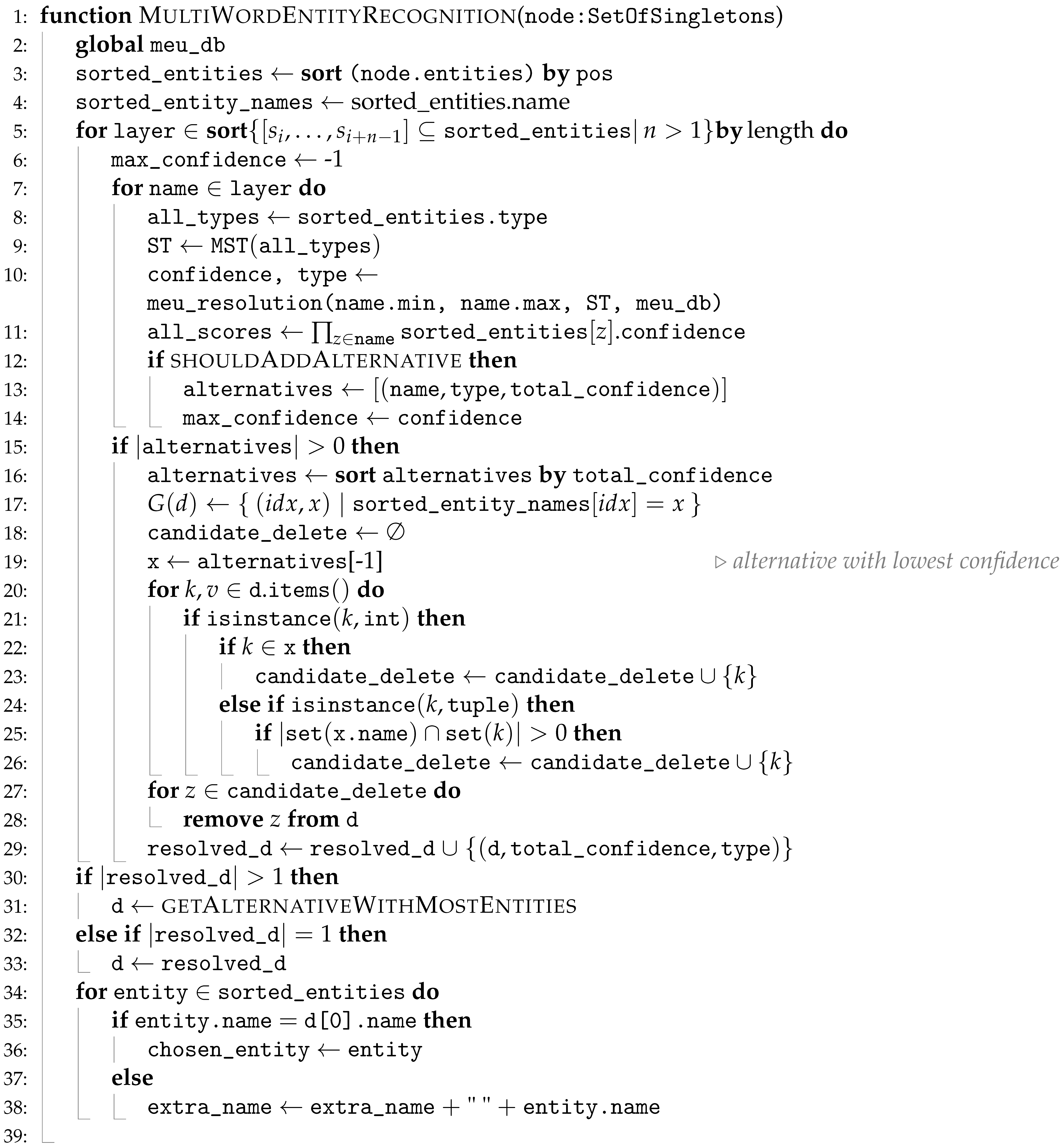
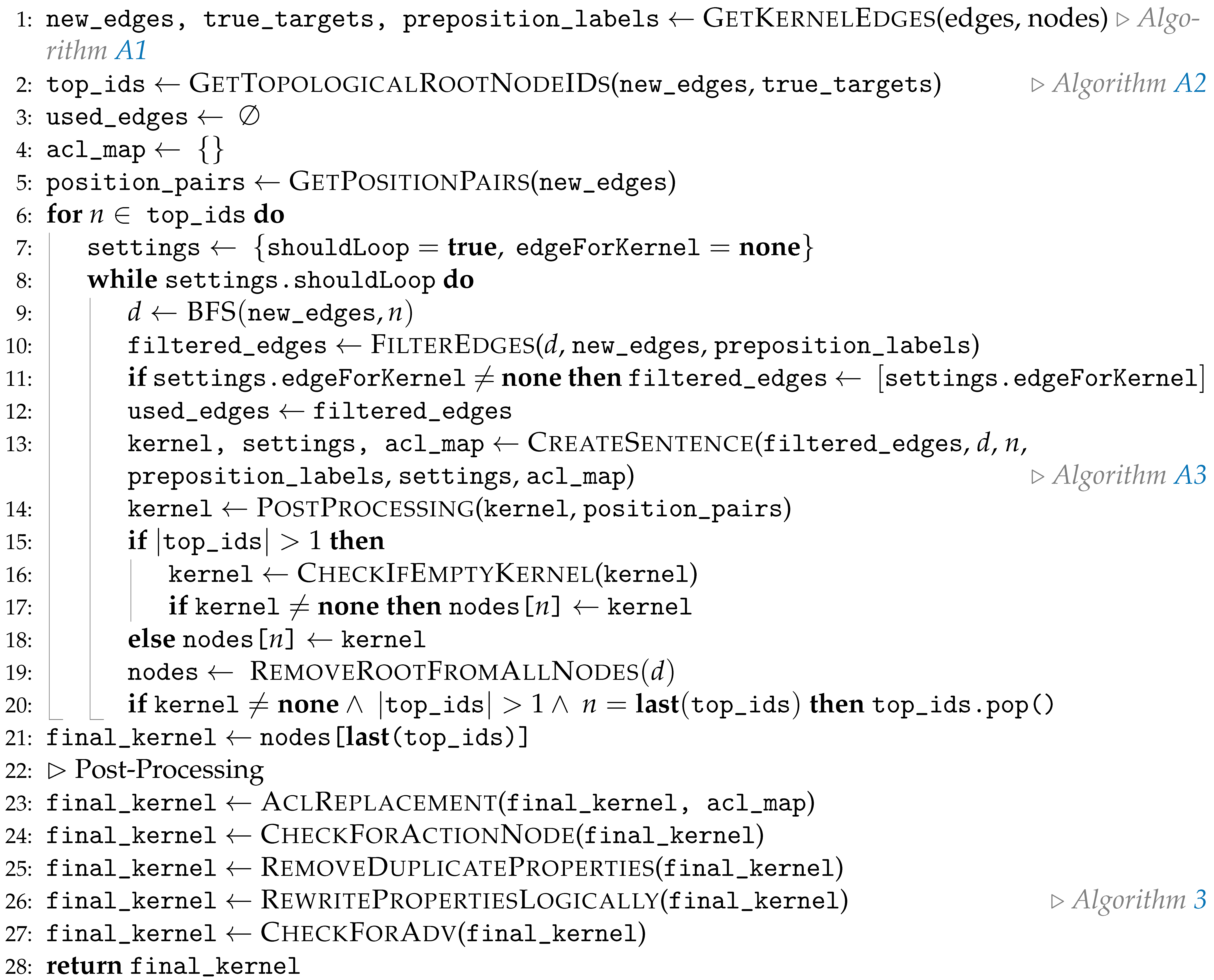
Funding

O.R.F.’s research is sponsored by a UK EPSRC PhD Studentship.

Institutional Review Board Statement

Not applicable.

Informed Consent Statement

Not applicable.

Data Availability Statement

The dataset is publicly available at https://osf.io/g5k9q/ (Accessed on 1 April 2025).

Conflicts of Interest

The authors declare no conflicts of interest.

Abbreviations

The following abbreviations are used in this manuscript:
AI Artificial Intelligence
BFS Breadth-First Search.
CWA Closed-World Assumption
DFS Depth-First Search
DG Dependency Graph
FOL First-Order Logic
GGG Generalised Graph Grammar
GPE GeoPolitical Entity
GQL Graph Query Language
GSM Generalised Semistructured Model
HAC Hierarchical Agglomerative Clustering
KB Knowledge Base
LaSSI Logical, Structural and Semantic text Interpretation
LR Logical Representation
MEU Multi-Word Entity Unit
meuDB Multi-Word Entity Unit DataBase
MG Montague Grammar
NLP Natural Language Processing
NN Neural Network
POS Part of Speech
QA Question Answering

Appendix A. Recursive Sentence Rewriting

We now describe with greater detail any subroutine required by Algorithm 2 to derive further subsequent computational steps.

Appendix A.1. Promoting Edges to Binary/Unary Relationships

Algorithm A1, collects all the appropriate edges to be considered when creating the kernel, and ensures that all edge labels to be considered are verbs and labels that are not verbs are disregarded. The first step in creating these kernels is getting all the appropriate edges, and determining which nodes within those edges are already roots, or should be considered if not already. This is presented on Line 1. Edges that are labelled with `dep’ are skipped on Line 7, as this type of edge is `impossible to determine a more precise relation’ [84], and therefore can be ignored. Next, we check every edge label for prototypical prepositions, retrieved from our ontology on Line 3, which determine target nodes to be roots, which are not already handled by dependency parsing. These prototypical prepositions are a single word (a preposition) that precedes a noun phrase complement, which expresses spatial relations [85]; for example: “the mouse is eatenbythe cat” or “charactersinmovies”. We check for whether our edge contains a prototypical preposition on Line 10: we want to determine if the preposition is contained within a wider edge label, but not exactly equal to; meaning if we had the label, “to steal”, this containsto”, so this would return true, however if we had “like”, this is exactly equal to, and therefore would return false. We also check for when the target does not contain a case property, as if we imply that a target with a case property is a sub-sentence, then we may lose additional information necessary for the logical rewriting phase in Section 3.3.4. We also do an additional check for whether the edge label ends with “ing” and does not contain an auxiliary as a condition for accepting as a true state for prototypical preposition. We do this so that sub-sentences can still be captured when a preposition is not contained within the full-text, but still introduced by a verb in its gerund form (-ing). We ensure that this does not contain an auxiliary so that we do not incorrectly say a new sentence is being introduced.
Algorithm A1:Construct Final Kernel
Preprints 154365 i0a1
If we find a preposition, we add a root property to the target node of the given edge, and map the target ID to the full edge label name in a prepositions list, to be used when determining which edge to use when creating the sentence in Algorithm A3.
There might be situations where roots are incorrectly identified, which is done on Line 16 by checking: if we have not found a preposition in the current edge label, the edge label is a verb, the source is a root, and the target is not an existential variable. If these conditions are all true, then the target’s root property (if present) is removed. We are removing something that is incorrectly recognised as a root, however this doesn’t affect verbs as in Algorithm A2, and on Line 5 will always return true if the given entity is a verb regardless of containing a root property.

Appendix A.2. Identifying the Clause Node Entry Points

Now that we have a list of all edges that should be considered for our given full-text, we need to find the IDs of the nodes that should be considered roots from which we generate all kernels. To do this, Algorithm A2 iterates over each source and target node within every edge collected from the previous step (Algorithm A1). Then, we filter each node by checking if they have a root property and not contained within the list of true targets to mitigate the chance of duplicate root IDs being added to filtered_nodes on Line 5. We also do an additional check for whether the node is a SetOfSingletons, and remove any node from the list that may be a child of the SetOfSingletons, as it would be incorrect to consider them roots as they are contained within the parent of the SetOfSingletons.
Algorithm A2:Construct Final Kernel (Algorithm 2 cont.)
Preprints 154365 i0a2
With the filtered_nodes collected, we need to sort them in topological order, so that when creating our logical representation, the structure is compliant with the original representation of the full-text. As we have performed a topological sort on the list of nodes when first parsing the GSM graph, we create a list of top_ids on Line 12. If we have not found any root nodes based on the filtering performed, then if only one node remains, this becomes our root node, otherwise we collect all nodes that have a root property as a fallback.

Appendix A.3. Generating Binary Relationships (Kernels)

To create our intermediate binary relationships, Algorithm A3 retrieves the node from the passed root_id (our n in Algorithm 2), and check for whether we have any edges to use in rewriting. If we do not have any edges, and the node is a verb, we create an `edge kernel’ on Line 5, which means that if we had the node `work’ with no other edges, then we return a kernel as such: work(?, None) as we have no further information at this stage. If it is not a verb, with no edges, then we simply return the node, as we cannot perform any rewriting.
Algorithm A3:Construct Final Relationship (Kernel) (Algorithm 2 cont.)
Preprints 154365 i0a3
If these conditions are not met then we assign our kernel, whereby we find the source, target and edge label to be used (Detailed in Algorithm A4). From this returned kernel, we create a list of kernel_nodes, which are the nodes to be considered before adding to the properties of the kernel, where if a property to be added is in the kernel_nodes, it should be ignored as the information is already contained in the entire kernel. Therefore we call a function to `analyse’ the source and target on Line 9, which adds the source and target to kernel_nodes.
Now, we iterate over each edge, e, and add the source and target nodes of each e to properties (Line 12). If a given e has an edge label equal to: `acl_relcl’, `nmod’, `nmod_poss’, then we rewrite this edge as a kernel within a Singleton (Line 15) and add the entire edge to the properties, to later be rewritten in Algorithm A5. If the edge label is `acl_relcl’, then we append this to the acl_map, used in Algorithm 2 on Line 23.
While iterating, we check on Line 17 for where e’s properties signify creating another kernel from the edges. If e is a verb and not already in the kernel_nodes, we use this edge in the next iteration within Algorithm A3 using the same root node; previousKernel is assigned to the current kernel at Line 27. We then check for this at Line 18 where we compare the current kernel and previous kernel, to determine if the previous kernel should become the root, or be added as a property; determined by the positions of each (Line 20).

Appendix A.3.1. Kernel Assignment

Algorithm A4: Construct Final Kernel (Algorithm A3 cont.)
Preprints 154365 i0a4
To `assign our kernel’, Algorithm A4 first needs to determine which edge is applicable for our current kernel on Line 3, by iterating over all the edges, to find our chosen_edge. We then iterate again over the edges, and once we reach either our chosen edge, or a verb when no chosen edge is found, we determine the attributes for our kernel. As long as our edge label is a verb, it remains the same, otherwise we use the source of the current e, given the condition on Line 6 our source becomes an existential (Line 10), otherwise it remains as the source of e. We then construct our kernel and check whether the edge label is a transitive verb or not (Section 2.3), and if it is not, then we remove the target as the target reflects the direct object.
If no kernel can be constructed, we look for an existential on Line 15, by checking the source and target for existential properties, and if we still cannot construct a kernel (where no existential is found), then we forcefully create the existential, by looking for a verb within the list of nodes on Line 17.
At this stage, we check if a case property is contained within the source or target, and if so we remove the node which is later appended as a property of the kernel. If the source is removed, it is replaced with an existential, if the target is removed it is replaced with none. If however, our target is a SetOfSingletons, then we look for a valid target within the entities target where we use the first occurring element by position in entities, and append the rest of the entities as properties (Line 23).

Appendix B. Rewriting Semantics for Logical Function Rules in Parmenides

Algorithm 3 from Section 3.3.4 shows how all properties for given kernel are rewritten, and encapsulates recursiveness for any given kernel by ensuring that properties of properties are accounted for. Each `key’ (typically) contains an array of entities, where n is each entity in the key, iterated across on Line 7. If n is a Singleton, we check that this contains a kernel and rewrite accordingly; if the node is an nmod or nmod_poss, then we do an additional check whereby if the rewritten property can be replaced within the source or target of the current kernel (k). On Line 4, we do a check for whether the key is extra, as this signifies that the current properties have already been logically rewritten, and therefore can be skipped. On Line 25, we create a new SetOfSingletons so long as the function on Line 21 returns a key_to_use. This will have an ID matching prop_node, and contain one element which is prop_node and a type which is the key from Line 3. For example, the sentence: “There is traffic but not in the Newcastle city centre” is initially: be(traffic, ?)[(AND:NOT(Newcastle[(extra:city centre), (6:in), (det:the)]))], so through Lines 19-23, as (6:in) is contained within Newcastle, this is rewritten to:
be(traffic, ?)[(SPACE:AND(NOT(Newcastle[(extra:city centre), (type:stay in place), (det:the)])))]
Algorithm A5: Logical Node Rewriting Function
Preprints 154365 i0a5
Algorithm A5 then rewrites a matched kernel according to the ontology information, as per the example in Listing Listing 7c. The algorithm returns properties with the (potentially) new `type key’, referring to the logical rewriting, that is then added to the kernel. The parameters passed in are the entire kernel, the initial_node being the node to be rewritten, properties which is the set of properties to be added to the entire kernel, has_nmod a Boolean from Line 11 in Algorithm 3, and return_key used for rewriting SetOfSingletons. Additional rules are also dealt with swapping the target with the properties, discussed in more detail in Section 5.4.

Appendix C. Classical Semantics, Bag Semantics, and Relational Algebra

Appendix C.1. Enumerating the Set of Possible Worlds Holding for a Formula

For relational algebra, we denote × as the cross product, ⋈ as the natural equi-join, σ P as the select/filter operator over a binary predicate P, and π L as the projection operator selecting only the attributes appearing in L. We define Calc f a s A ( T ) as the non-classical relational algebra operator extending the relational table T with a new attribute A while extending each tuple ( v 1 , , v n ) T via f as ( v 1 , , v n , f ( v 1 , , v n ) ) . Given a logical formula φ ( s ) and some truth assignments to logical predicates through a function Γ , we denote [ [ φ ( s ) ] ] ( Γ ) as the valuation function computed over of φ ( s ) via the truth assignments in Γ .
After determining all the binary or unary predicates a 1 , , a n associated to a Logical Representation (LR) φ ( s ) of a factoid sentence s, we derive a truth table T s ( a 1 , , a n , s ) for φ ( s ) represented as a relational table T s = Calc [ [ φ ( s ) ] ] a s s ( × a i { a 1 , , a n } { 0 , 1 } ) by assuming each proposition to be completely independent from the other without any further background knowledge.

Appendix C.2. Knowledge-Based Driven Propositional Semantics

Walking on the footsteps of our previous research [5], we derive the following conditions out of which we discretise the notion of logical implication between propositions and their properties:
Definition A1. (Multi-Valued Semantics).
Given a KB K , we say that two propositions or properties are equivalent ( Eq ) if either they satisfy the structural equivalence ≡ formally defined as Leibniz equivalence [86] or if they appear within a transitive closure of equivalence relationships in K . We also say that these are mutually exclusives ( NEq ) if either one of the two is a negation and its argument is Leibniz equivalent ot the other, or after a transitive closure of equivalence or logical implications, we derive that one argument is mutually exclusive in K . Then, we distinguish multiple types of logical implications by considering the structure of the proposition extended with data properties:
nspec :
If we lose specificity due to some missing copula information.
None :
By interpreting a missing value from one of the property arguments as a missing information entailing any possible value for this field, whether the right element is a non-missing value.
:
If we interpret the second object as being a specific instance of the first one.
↠:
A general implication state that cannot be easily categorised by any of the former cases while including any of the former.
If neither of the above applies, then we state that the two propositions or properties are indifferent, and we denote them with ω. We denote any generic implication relationship as .

Appendix C.2.1. Multi-Valued Term Equivalence

Please observe that, differently from standard logic literature, we also consider the negation of terms, implicitly entailing any term being different from the one specified. This shorthand is required as human lanuguage not only expresses negations over entire propositions or formulæ, but also on single terms.
When the assessment of multi-valued semantics between two items a and b is determined through a KB K , we denote this as a K b the outcome of such comparison. In the forthcoming steps, we provide the definitions for the notion of equivalence derivable from the analysis of the structural properties of the propositions and their terms through the KB values given above. The transform when negated function η ( v ) implements the intended semantics of the negation of a multi-valued semantics comparison value: Eq becomes NEq and vice versa, while all other remaining cases are mapped to ω otherwise, as the negation of an implication does not necessarily entail non-implication, and no further information can be derived. The following definition offers a first definition of term equivalence encompassing the name associated with it, potential specifications associated with them, as well as adjectives genereally referred to as copulæ:
Definition A2. (Term Equivalence).
Given a KB K of interest, we denote the discrete notion of term equivalence as follows:
a ter b = Eq a b c = n = s NEq a ¬ b b ¬ a η ( a ter b ) a ¬ a η ( a ter b ) b ¬ b None a None ω b None ¬ isTerm ( a ) ¬ isTerm ( b ) n = ω b . all a . all n c ˜ = Eq a . name None b . specification None n = ω b . all ¬ a . all n c ˜ = Eq a . name None b . specification None n ˜ n = ω b . all ¬ a . all n ˜ = n = ω ¬ b . all ¬ a . all n ˜ = Eq s n = Eq s = c ( b . all = a . all b . all ) nspec n = s = Eq c = None c n = Eq n n = s = c = Eq ¬ b . all a . all NEq n = s = Eq c = NEq n = n c ˜ = Eq b . specification = None b . all NEq n = NEq f = c = Eq ω oth .
where we use c as a shorthand for the comparison between copulæ occurring within flipped terms b . cop var a . cop , n as a shorthand for the name comparison within terms a . name K b . name , s as a shorthand for the specification comparison within terms b . specification K a . specification , n c as a shorthand of the comparison between name and specification a . name var b . specification . Given any of the former symbol x, we denote as x ˜ the flipped variant of the former where the first and second argument are swapped, while always referring to the same arguments (e.g., n c ˜ = b . name var a . specification ).

Appendix C.2.2. Multi-Valued Proposition Equivalence

First, we can consider the equivalence of propositions by types, while ignoring their property arguments p and p : while for unary propositions this boils down to the sole argument’s term equivalence (Eq. A2), for the binary predicates, by implicitly consider them as a functional dependency of the first argument over the second, we consider them according to this priority order (Eq. A3). In both cases, if the propositions differ by the relationship name, we ignore the comparison with ω .
r p ( s ) un r p ( s ) = ω r r s ter s o t h .
r p ( s , d ) bin r p ( s , d ) = ω ( r r ) ( s ter s = ω ) ( t ter t = ω ) ω ( s ter s = NEq ) ( t ter t = NEq ) NEq ( s ter s = NEq ) ( t ter t ω ) NEq ( t ter t = NEq ) ( s ter s ω ) s ter s t ter t = Eq t ter t s ter s = Eq ς ( { s ter s , t ter t } ) oth .
Given a set of comparison outcomes S referring to comparison outcomes of terms referring to the same key within a property, we define σ as the function simplifying the comparison outcomes with the most specific multi-valued equivalence output summarising the evidence being collected so far:
ς ( S ) = ω S = NEq NEq S Eq Eq S nspec nspec S None S S S None nspec S None S S S nspec S None S S S nspec S None S S S
We also define another function ς for summarising these considerations further across all key values within the same property; the purpose of this second function is to provide the general notion of proposition similarity at the level of the properties, and where the main difference relies on the order of the application of the rules. If both properties have no propoerties, they are deemed equivalent on those premises:
ς ( S ) = Eq S = ω ω S NEq NEq S ς ( S ) Eq S ( nspec S None S S S ) Eq Eq S ω o t h .
After this, we can define two functions, summarising the implication relationships within properties p and p for the first and second proposition respectively: κ r considers the verse of the implication from the first term towards the second (Eq. A6), while κ i considers the inverse order (Eq. A7):
κ r ( p , p ) = [ k ς ( { a ter b | a p ( k ) , b p ( b ) } ) ] k dom ( p ) dom ( p ) [ k ω ] k dom ( p ) k dom ( p ) [ k ] k dom ( p ) k dom ( p )
κ i ( p , p ) = [ k ς ( { a ter b | a p ( k ) , b p ( b ) } ) ] k dom ( p ) dom ( p ) [ k ] k dom ( p ) k dom ( p ) [ k ω ] k dom ( p ) k dom ( p )
, κ ς ( cod ( κ i ( p , p ) ) )
Given these ancillary definitions, we can now define the can now define the definition of the discrete equivalence between propositions occurring within the formula:
Definition A3.
Given a KB K and two propositions a or b, where the first is associated with a property p and the second with a property p , we can define the following discrete equivalence function:
a prop b = Eq a b NEq a ¬ b b ¬ a η ( a prop b ) a ¬ a η ( a prop b ) b ¬ b ω a None b None a prop b a ¬ a b ¬ b ( a prop b ) ω a ¬ a b ¬ b ( a prop b ) = ω isBinary ( a ) isBinary ( b ) ω a = r ( t 1 ) b = r ( t 2 ) t 1 t 2 ω γ = ω κ γ = Eq f = Eq κ = c Eq ω γ = Eq f = Eq κ = c = Eq ω cod ( κ r ( p , p ) ) ω γ = Eq f = Eq κ = c = Eq nspec cod ( κ r ( p , p ) ) κ γ = Eq f = Eq ( κ = cod ( κ r ( p , p ) ) ) ω γ = Eq f = Eq κ = o t h . γ = Eq f = Eq κ = nspec κ γ = Eq f = Eq κ nspec κ ω γ = κ Eq ω κ r ( p , p ) γ = κ Eq κ = nspec κ γ = κ Eq κ nspec ω κ r ( p , p ) ω γ = ( κ = ω κ = ) γ o t h .
where γ is a shorthand for the comparison outcome between either binary ( a bin b ) or unary ( a un b ) propositions, f is a shorthand for the comparison of the first argument considered as a term ( s ter s ), c is a comparison of the first arguments’ copulæif occurring ( s . cop ter s . cop ), κ summarises the comparison between the first proposition’s properties with the one of the second ( ς ( cod ( κ r ( p , p ) ) ) ), while κ flips such comparison ( κ ς ( cod ( κ r ( p , p ) ) ) ).

Appendix D. Proofs

Proof(for Lemma 13).
Given a binary relationship x y ( x , y ) , symmetry is a property of , where if x and y are related in either direction, then x and y are equivalent. Formally: Due to the commutative property of the dot product, S c ( A , B ) = S c ( B , A ) [87]. □
Proof(for Lemma 14).
If B implies A under a symmetric metric S , then A also implies B. This is because the similarity value remains the same regardless of the order of arguments. Formally:
φ τ ( β , α ) S ( τ ( β ) , τ ( α ) ) > θ ( by Definition , θ ¯ ) S ( τ ( α ) , τ ( β ) ) > θ ( by Lemma , s y m m ) φ τ ( α , β ) ( by Definition )
Proof (for Lemma 15).
Left to right: If two equations are the same, they will have the same set of the possible worlds. Given this, their intersection will be always equivalent to one of the two sets, from which it derives that the support of either of the two formulas is always true.
W ( A ) = W ( B ) W ( A ) W ( B ) = W ( A ) | W ( A ) W ( B ) | | W ( A ) | = 1
Right to left: When the confidence is 1, then by definition both the numerator and denominator are of the same size. Therefore | W ( A ) W ( B ) | = | W ( A ) | and | W ( B ) W ( A ) | = | W ( B ) | . By the commutativity of the intersection, we then derive that | A | | B | are of the same size and represent the same set. Thus, it holds that A B .
Proof(for Corollary 16).
The following notation implies that; if it exists for an x that belongs to W ( A ) and not to W ( B ) , then their intersection size will be less than the size of A, and if W ( A ) W ( B ) has less items of W ( A ) , then it entails that B contains elements not occurring in A:
x . x W ( A ) x W ( B ) | W ( A ) W ( B ) | < | W ( A ) | confidence ( A , B ) < 1
Then, we want to characterise which is the logical formula supporting a set of elements belonging to A but not to B. We can derive this from the bag semantics of our logical operators, and infer that the below condition holds when A does not necessarily imply B:
W ( ¬ ( A B ) ) = S = W ( A ¬ B ) = W ( A ) W ( B )
∴ when A holds B doesn’t necessarily hold. □

References

  1. Tammet, T.; Järv, P.; Verrev, M.; Draheim, D. An Experimental Pipeline for Automated Reasoning in Natural Language (Short Paper). In Proceedings of the Automated Deduction – CADE 29; Pientka, B., Tinelli, C., Eds.; Cham, 2023; pp. 509–521. [Google Scholar]
  2. Hicks, M.T.; Humphries, J.; Slater, J. ChatGPT is bullshit. Ethics and Information Technology 2024, 26, 38. [Google Scholar] [CrossRef]
  3. Bender, E.M.; Gebru, T.; McMillan-Major, A.; Shmitchell, S. On the Dangers of Stochastic Parrots: Can Language Models Be Too Big? In Proceedings of the Proceedings of the 2021 ACM Conference on Fairness, Accountability, and Transparency, New York, NY, USA, 2021; FAccT ’21. pp. 610–623. [Google Scholar]
  4. Chen, Y.; Wang, D.Z. Knowledge expansion over probabilistic knowledge bases. In Proceedings of the International Conference on Management of Data, SIGMOD 2014, Snowbird, UT, USA, 22-27 June 2014; Dyreson, C.E., Li, F., Özsu, M.T., Eds.; ACM, 2014; pp. 649–660. [Google Scholar]
  5. Bergami, G. A framework supporting imprecise queries and data. CoRR 2019, abs/1912.12531. [Google Scholar]
  6. Kyburg, H.E. Probability and the Logic of Rational Belief; Wesleyan University Press: Middletown, CT, USA, 1961. [Google Scholar]
  7. Brown, B. Inconsistency measures and paraconsistent consequence. In Measuring Inconsistency in Information; Grant, J., Martinez, M.V., Eds.; College Press, 2018; chapter 8; pp. 219–234. [Google Scholar]
  8. Graydon, M.S.; Lehman, S.M. Examining Proposed Uses of LLMs to Produce or Assess Assurance Arguments; NTRS - NASA Technical Reports Server.
  9. Dallachiesa, M.; Ebaid, A.; Eldawy, A.; Elmagarmid, A.; Ilyas, I.F.; Ouzzani, M.; Tang, N. NADEEF: a commodity data cleaning system. In Proceedings of the 2013 ACM SIGMOD International Conference on Management of Data, New York, NY, USA, 2013; SIGMOD ’13. pp. 541–552. [Google Scholar]
  10. Andrzejewski, W.; Bębel, B.; Boiński, P.; Wrembel, R. On tuning parameters guiding similarity computations in a data deduplication pipeline for customers records: Experience from a R&D project. Information Systems 2024, 121, 102323. [Google Scholar]
  11. Picado, J.; Davis, J.; Termehchy, A.; Lee, G.Y. Learning Over Dirty Data Without Cleaning. In Proceedings of the 2020 International Conference on Management of Data, SIGMOD Conference 2020, online conference, Portland, OR, USA, 14-19 June 2020; Maier, D., Pottinger, R., Doan, A., Tan, W., Alawini, A., Ngo, H.Q., Eds.; ACM, 2020; pp. 1301–1316. [Google Scholar]
  12. Virgilio, R.D.; Maccioni, A.; Torlone, R. Approximate querying of RDF graphs via path alignment. Distributed Parallel Databases 2015, 33, 555–581. [Google Scholar] [CrossRef]
  13. Tenghao, J. FAQ question Answering method based on semantic similarity matching. In Proceedings of the ISCSIC; 2022; pp. 93–100. [Google Scholar]
  14. He, X.; Tian, Y.; Sun, Y.; Chawla, N.V.; Laurent, T.; LeCun, Y.; Bresson, X.; Hooi, B. G-Retriever: Retrieval-Augmented Generation for Textual Graph Understanding and Question Answering. [CrossRef]
  15. Zhang, T. GAIA - A Multi-media Multi-lingual Knowledge Extraction and Hypothesis Generation System. In Proceedings of the Proceedings of the 2018 Text Analysis Conference, TAC 2018, NIST, 2018. Gaithersburg, Maryland, USA, 13-14 November 2018. NIST, 2018. [Google Scholar]
  16. Fox, O.R.; Bergami, G.; Morgan, G. LaSSI: Logical, Structural, and Semantic text Interpretation. In Proceedings of the Database Engineered Applications; Springer, 2025. IDEAS ’24 (in press) [Google Scholar]
  17. Wong, P.C.; Whitney, P.; Thomas, J. Visualizing Association Rules for Text Mining. In Proceedings of the 1999 IEEE Symposium on Information Visualization, USA, 1999; INFOVIS ’99. p. 120.
  18. Speer, R.; Chin, J.; Havasi, C. ConceptNet 5.5: An Open Multilingual Graph of General Knowledge. In Proceedings of the Thirty-First AAAI Conference on Artificial Intelligence, San Francisco, CA, USA, 4-9 February 2017; Singh, S., Markovitch, S., Eds.; AAAI Press, 2017; pp. 4444–4451. [Google Scholar] [CrossRef]
  19. Seshia, S.A.; Sadigh, D.; Sastry, S.S. Toward verified artificial intelligence. Commun. ACM 2022, 65, 46–55. [Google Scholar] [CrossRef]
  20. Li, F.; Jagadish, H.V. NaLIR: an interactive natural language interface for querying relational databases. In Proceedings of the 2014 ACM SIGMOD International Conference on Management of Data, New York, NY, USA, 2014; SIGMOD ’14. pp. 709–712. [Google Scholar] [CrossRef]
  21. Bergami, G.; Fox, O.R.; Morgan, G. Extracting Specifications through Verified and Explainable AI: Interpretability, Interoperabiliy, and Trade-offs (In Press). In Explainable Artificial Intelligence for Trustworthy Decisions in Smart Applications; Springer; chapter 2.
  22. Sun, X. Structure Regularization for Structured Prediction. In Proceedings of the Advances in Neural Information Processing Systems 27: Annual Conference on Neural Information Processing Systems, Montreal, Quebec, Canada, 8-13 December 2014; Ghahramani, Z., Welling, M., Cortes, C., Lawrence, N.D., Weinberger, K.Q., Eds.; 2014; pp. 2402–2410. [Google Scholar]
  23. Manning, C.; Surdeanu, M.; Bauer, J.; Finkel, J.; Bethard, S.; McClosky, D. The Stanford CoreNLP Natural Language Processing Toolkit. In Proceedings of the 52nd Annual Meeting of the Association for Computational Linguistics: System Demonstrations; Bontcheva, K., Zhu, J., Eds.; Baltimore, Maryland, June 2014; pp. 55–60. [Google Scholar] [CrossRef]
  24. et. al, J.N. conj. Available online: https://universaldependencies.org/en/dep/conj.html (accessed on 13 February 2025).
  25. et. al, J.N. cc. Available online: https://universaldependencies.org/en/dep/cc.html (accessed on 13 February 2025).
  26. Jurafsky, D.; Martin, J.H. Speech and Language Processing: An Introduction to Natural Language Processing, Computational Linguistics, and Speech Recognition with Language Models, 3rd ed.12 January 2025; Online manuscript released January 12, 2025. [Google Scholar]
  27. Group, S.N.
  28. Cardona, G. Pāṇini – His Work and its Traditions, 2 ed.; Vol. 1, Motilal Banarsidass: London, 1997. [Google Scholar]
  29. Christensen, C.H. Arguments for and against the Idea of Universal Grammar. Leviathan: Interdisciplinary Journal in English 2019, 12–28. [Google Scholar] [CrossRef]
  30. Hauser, M.D.; Chomsky, N.; Fitch, W.T. The Faculty of Language: What Is It, Who Has It, and How Did It Evolve? Science 2002, 298, 1569–1579. [Google Scholar] [CrossRef]
  31. Montague, R. ENGLISH AS A FORMAL LANGUAGE. In Logic and philosophy for linguists; De Gruyter Mouton: Berlin, Boston, 1975; pp. 94–121. [Google Scholar] [CrossRef]
  32. Montague, R. English as a formal language. In Linguaggi nella Societa e nella Tecnica; Edizioni di Communità: Milan, Italy, 1970; pp. 189–224. [Google Scholar]
  33. Dardano, M.; Trifone, P. Italian grammar with linguistics notions (in Italian); Zanichelli: Milan, 2002. [Google Scholar]
  34. terdon. terminology - Syntactic analysis in English: correspondence between Italian complements and English ones, url=https://english.stackexchange.com/questions/628592/syntactic-analysis-in-english-correspondence-between-italian-complements-and/628597#628597, urldate=10.02.2025.
  35. Bergami, G.; Fox, O.R.; Morgan, G. Matching and Rewriting Rules in Object-Oriented Databases. Mathematics 2024, 12. [Google Scholar] [CrossRef]
  36. et. al, J.N. English Dependency Relations. Available online: https://universaldependencies.org/en/dep/ (accessed on 24 February 2025).
  37. Ahlers, D. Assessment of the accuracy of GeoNames gazetteer data. In Proceedings of the Proceedings of the 7th Workshop on Geographic Information Retrieval, New York, NY, USA, 2013; GIR ’13. pp. 74–81. [Google Scholar]
  38. Chang, A.X.; Manning, C. SUTime: A library for recognizing and normalizing time expressions. In Proceedings of the Eighth International Conference on Language Resources and Evaluation (LREC`12); Calzolari, N., Choukri, K., Declerck, T., Doğan, M.U., Maegaard, B., Mariani, J., Moreno, A., Odijk, J., Piperidis, S., Eds.; Istanbul, Turkey, 2012; pp. 3735–3740. [Google Scholar]
  39. Qi, P.; Zhang, Y.; Zhang, Y.; Bolton, J.; Manning, C.D. Stanza: A Python Natural Language Processing Toolkit for Many Human Languages. In Proceedings of the 58th Annual Meeting of the Association for Computational Linguistics: System Demonstrations; 2020. [Google Scholar]
  40. Speer, R.; Chin, J.; Havasi, C. ConceptNet 5.5: an open multilingual graph of general knowledge. In Proceedings of the AAAI; AAAI Press, 2017. AAAI’17. pp. 4444–4451. [Google Scholar]
  41. Group, T.P.G.D. PostgreSQL: Documentation: 17: F.16. fuzzystrmatch — determine string similarities and distanceAppendix F. Additional Supplied Modules and Extensions. Available online: https://www.postgresql.org/docs/current/fuzzystrmatch.html (accessed on 18.02.2025).
  42. Bergami, G.; Zegadło, W. Towards a Generalised Semistructured Data Model and Query Language. SIGWEB Newsl. 2023, 2023. [Google Scholar] [CrossRef]
  43. Bonifati, A.; Murlak, F.; Ramusat, Y. Transforming Property Graphs. 2024; arXiv:cs.DB/2406.13062. [Google Scholar]
  44. Bergami, G.; Fox, O.R.; Morgan, G. Matching and Rewriting Rules in Object-Oriented Databases. Preprints 2024. [Google Scholar] [CrossRef]
  45. 2025, C.U.P..A. Modality: forms - Grammar - Cambridge Dictionary. Available online: https://dictionary.cambridge.org/grammar/british-grammar/modality-forms#:~:text=Dare%2C%20need%2C%20ought%20to%20and%20used%20to%20 (accessed on 17 March 2025).
  46. et. al, J.N. case. Available online: https://universaldependencies.org/en/dep/case.html (accessed on 5 March 2025).
  47. et. al, J.N. case. Available online: https://universaldependencies.org/en/dep/nmod.html (accessed on 5 March 2025).
  48. Jatnika, D.; Bijaksana, M.A.; Suryani, A.A. Word2Vec Model Analysis for Semantic Similarities in English Words. In Proceedings of the Enabling Collaboration to Escalate Impact of Research Results for Society: The 4th International Conference on Computer Science and Computational Intelligence, ICCSCI 2019, Yogyakarta, Indonesia, 12-13 September 2019; Budiharto, W., Ed.; Elsevier, 2019; 157, Procedia Computer Science. pp. 160–167. [Google Scholar] [CrossRef]
  49. Mikolov, T.; Chen, K.; Corrado, G.; Dean, J. Efficient Estimation of Word Representations in Vector Space. In Proceedings of the 1st International Conference on Learning Representations, ICLR 2013, Scottsdale, Arizona, USA, 2-4 May 2013; Workshop Track Proceedings. Bengio, Y., LeCun, Y., Eds.; [Google Scholar]
  50. Rosenberger, J.; Wolfrum, L.; Weinzierl, S.; Kraus, M.; Zschech, P. CareerBERT: Matching resumes to ESCO jobs in a shared embedding space for generic job recommendations. Expert Systems with Applications 2025, 275, 127043. [Google Scholar] [CrossRef]
  51. Liu, H.; Bao, H.; Xu, D. Concept Vector for Similarity Measurement Based on Hierarchical Domain Structure. Comput. Informatics 2011, 30, 881–900. [Google Scholar]
  52. Nickel, M.; Kiela, D. Poincaré Embeddings for Learning Hierarchical Representations. In Proceedings of the Advances in Neural Information Processing Systems 30: Annual Conference on Neural Information Processing Systems 2017, Long Beach, CA, USA, 4-9 December 2017; Guyon, I., von Luxburg, U., Bengio, S., Wallach, H.M., Fergus, R., Vishwanathan, S.V.N., Garnett, R., Eds.; 2017; pp. 6338–6347. [Google Scholar]
  53. Raedt, L.D. Logical and Relational Learning; Springer-Verlag: Berlin Heidelberg, 2008. [Google Scholar]
  54. Asperti, A.; Ciabattoni, A. Logica ad Informatica.
  55. Simard, P.Y.; Amershi, S.; Chickering, D.M.; Pelton, A.E.; Ghorashi, S.; Meek, C.; Ramos, G.A.; Suh, J.; Verwey, J.; Wang, M.; et al. Machine Teaching: A New Paradigm for Building Machine Learning Systems. CoRR, 2017; arXiv:abs/1707.06742. [Google Scholar]
  56. Ramos, G.; Meek, C.; Simard, P.; Suh, J.; and, S.G. Interactive machine teaching: a human-centered approach to building machine-learned models. Human–Computer Interaction 2020, 35, 413–451. [Google Scholar] [CrossRef]
  57. Mosqueira-Rey, E.; Hernández-Pereira, E.; Alonso-Ríos, D.; Bobes-Bascarán, J.; Fernández-Leal, Á. Human-in-the-loop machine learning: a state of the art. Artificial Intelligence Review 2023, 56, 3005–3054. [Google Scholar] [CrossRef]
  58. Bergami, G. A new Nested Graph Model for Data Integration. Ph.D. thesis, University of Bologna, Bologna, Italy, 2018. [Google Scholar] [CrossRef]
  59. Carnielli, W.; Esteban Coniglio, M. Paraconsistent Logic: Consistency, Contradiction and Negation; Springer: Switzerland, 2016. [Google Scholar]
  60. Hinman, P.G. Fundamentals of Mathematical Logic; A K Peters/CRC Press, 2005. [Google Scholar]
  61. Kleene, S.C. Introduction to Metamathematics; P. Noordhoff N.V.: Groningen, 1952. [Google Scholar]
  62. Strobl, L.; Merrill, W.; Weiss, G.; Chiang, D.; Angluin, D. What Formal Languages Can Transformers Express? A Survey. Transactions of the Association for Computational Linguistics 2024, 12, 543–561. [Google Scholar] [CrossRef]
  63. Hugging Face. sentence-transformers (Sentence Transformers). Available online: https://huggingface.co/sentence-transformers (accessed on 24 February 2025).
  64. Wang, W.; Wei, F.; Dong, L.; Bao, H.; Yang, N.; Zhou, M. MiniLM: Deep Self-Attention Distillation for Task-Agnostic Compression of Pre-Trained Transformers. 2020; arXiv:cs.CL/2002.10957. [Google Scholar]
  65. Song, K.; Tan, X.; Qin, T.; Lu, J.; Liu, T.Y. MPNet: Masked and Permuted Pre-training for Language Understanding. 2020; arXiv:cs.CL/2004.09297. [Google Scholar]
  66. Liu, Y.; Ott, M.; Goyal, N.; Du, J.; Joshi, M.; Chen, D.; Levy, O.; Lewis, M.; Zettlemoyer, L.; Stoyanov, V. MPNet: Masked and Permuted Pre-training for Language Understanding. 2019; arXiv:cs.CL/1907.11692. [Google Scholar]
  67. Defays, D. An efficient algorithm for a complete link method. The Computer Journal 1977, 20, 364–366. [Google Scholar] [CrossRef]
  68. Nielsen, F. , 2016; pp. 195–211. https://doi.org/10.1007/978-3-319-21903-5_8.Clustering. In Introduction to HPC with MPI for Data Science; Springer International Publishing: Cham, 2016; pp. 195–211. [Google Scholar] [CrossRef]
  69. Zaki, M.J.; Meira, W., Jr. Data Mining and Machine Learning: Fundamental Concepts and Algorithms, 2nd ed.; Cambridge University Press, 2020. [Google Scholar]
  70. Partitioning Around Medoids (Program PAM). In Finding Groups in Data; John Wiley & Sons, Ltd, 1990; chapter 2, pp. 68–125, [https://onlinelibrary.wiley.com/doi/pdf/10.1002/9780470316801.ch2]. [CrossRef]
  71. Arthur, D.; Vassilvitskii, S. k-means++: the advantages of careful seeding. In Proceedings of the Proceedings of the Eighteenth Annual ACM-SIAM Symposium on Discrete Algorithms, SODA 2007, New Orleans, Louisiana, USA, 7-9 January 2007; Bansal, N., Pruhs, K., Stein, C., Eds.; SIAM, 2017; pp. 1027–1035. [Google Scholar]
  72. O’Neil, E.J.; O’Neil, P.E.; Weikum, G. The LRU-K Page Replacement Algorithm For Database Disk Buffering. In Proceedings of the 1993 ACM SIGMOD International Conference on Management of Data, Washington, DC, USA, 26-28 May 1993; ACM Press, 1993; pp. 297–306. [Google Scholar] [CrossRef]
  73. Johnson, T.; Shasha, D.E. 2Q: A Low Overhead High Performance Buffer Management Replacement Algorithm. In Proceedings of the VLDB’94, Proceedings of 20th International Conference on Very Large Data Bases, Santiago de Chile, Chile, 12-15 September 1994; Bocca, J.B., Jarke, M., Zaniolo, C., Eds.; Morgan Kaufmann, 1994; pp. 439–450. [Google Scholar]
  74. Brown, T.B.; Mann, B.; Ryder, N.; Subbiah, M.; Kaplan, J.; Dhariwal, P.; Neelakantan, A.; Shyam, P.; Sastry, G.; Askell, A.; et al. Language Models are Few-Shot Learners. CoRR 2020, arXiv:abs/2005.14165. [Google Scholar]
  75. Harrison, J. Handbook of Practical Logic and Automated Reasoning; Cambridge University Press, 2009. [Google Scholar]
  76. Chen, D.; Manning, C.D. A Fast and Accurate Dependency Parser using Neural Networks. In Proceedings of the 2014 Conference on Empirical Methods in Natural Language Processing, EMNLP 2014, Doha, Qatar, 25-29 October 2014; A meeting of SIGDAT, a Special Interest Group of the ACL. Moschitti, A., Pang, B., Daelemans, W., Eds.; 2014; pp. 740–750. [Google Scholar] [CrossRef]
  77. Kruskal, J.B.; Wish, M. Multidimensional Scaling; Quantitative Applications in the Social Sciences, SAGE Publications, Inc.
  78. Mead, A. Review of the Development of Multidimensional Scaling Methods. Journal of the Royal Statistical Society. Series D (The Statistician) 1992, 41, 27–39. [Google Scholar] [CrossRef]
  79. Agarwal, S.; Wills, J.; Cayton, L.; Lanckriet, G.R.G.; Kriegman, D.J.; Belongie, S.J. Generalized Non-metric Multidimensional Scaling. In Proceedings of the Eleventh International Conference on Artificial Intelligence and Statistics, AISTATS 2007, San Juan, Puerto Rico, 21-24 March 2007; Meila, M., Shen, X., Eds.; JMLR.org. 2007; 2, JMLR Proceedings. pp. 11–18. [Google Scholar]
  80. Quist, M.; Yona, G. Distributional Scaling: An Algorithm for Structure-Preserving Embedding of Metric and Nonmetric Spaces. J. Mach. Learn. Res. 2004, 5, 399–420. [Google Scholar]
  81. Costa, C.F.; Nascimento, M.A.; Schubert, M. Diverse nearest neighbors queries using linear skylines. GeoInformatica 2018, 22, 815–844. [Google Scholar] [CrossRef]
  82. Botea, V.; Mallett, D.; Nascimento, M.A.; Sander, J. PIST: An Efficient and Practical Indexing Technique for Historical Spatio-Temporal Point Data. GeoInformatica 2008, 12, 143–168. [Google Scholar] [CrossRef]
  83. Hopcroft, J.E.; Ullman, J.D. Introduction to Automata Theory, Languages and Computation; Addison-Wesley, 1979. [Google Scholar]
  84. et. al, J.N. dep. Available online: https://universaldependencies.org/en/dep/dep.html (accessed on 27 February 2025).
  85. Weber, D. English Prepositions in the History of English Grammar Writing. AAA: Arbeiten aus Anglistik und Amerikanistik 2012, 37, 227–243. [Google Scholar]
  86. Asperti, A.; Ricciotti, W.; Sacerdoti Coen, C. Matita Tutorial. Journal of Formalized Reasoning 2014, 7, 91–199. [Google Scholar] [CrossRef]
  87. Nykamp, D.Q. The dot product.
Figure 1. Visualisation of the main difference between POS tagging (below) and ud (above), providing more explicit relationships between words.
Preprints 154365 g001
Figure 2. Example of a recursive sentence, highlighted by each coloured bounding box.
Preprints 154365 g002
Figure 3. LaSSI Pipeline: Operational description of the pipeline.
Preprints 154365 g003
Figure 4. GSM output for “Traffic is flowing in Newcastle city centre, on Saturdays”.
Preprints 154365 g004
Figure 5. Stages of transformation for a full-text: “Newcastle and Brighton have traffic”.
Preprints 154365 g005
Figure 6. Example graph after the GSM rewriting for the sentence “become able to answer more questions” with node IDs overlayed in the middle of each node.
Preprints 154365 g006
Figure 7. Fragments of the Parmenides ontology encoding rules for capturing Logical Functions from
Preprints 154365 g007
Figure 8. Truth tables over admissible and compatible worlds for implying, indifferent, inconsistent, and equivalent atoms.
Preprints 154365 g008
Figure 15. Plot of scalability tests for the LaSSI pipeline in log-norm scale.
Preprints 154365 g015
Figure 16. Graph inputs (StanfordNLP) and outputs (GSM rewriting) for three sentences.
Preprints 154365 g016
Figure 17. Input graph from StanfordNLP for the sentence: “making you angry”.
Preprints 154365 g017
Figure 18. GSM output from our old pipeline [16] for, “Traffic is flowing in Newcastle city centre, on Saturdays”, where multipleindobj is missing from the graph, which was added in our new pipeline to reify n-ary relationships into a SetOfSingletons (Figure 4).
Preprints 154365 g018
Table 1. Some examples of Logical Functions considered in the current LaSSI pipeline beyond the simple subject-verb-direct object categorisation. These are then categorised and explained in our Parmenides ontology (Section 3.3.4), where these are not only defined by the POS tags and the prepositions associated with them, but also on the type of verb and entity associated with it.
Logical Function (Sub)Type Example (underlined)
Space Stay in place I sit on a tree.
Space Motion to place I go to Bologna.
Space Motion from place I come from Italy.
Space Motion through place Going across the city center.
Cause Newcastle is closed for congestion
Time Continuous The traffic lasted for hours
Time Defined On Saturdays, traffic is flowing
Table 2. Truth table of values for sentences α and β .
#W p 1 p 2 A : p 1 p 2 B : p 1 p 2
#1 0 0 0 0
#2 0 1 0 1
#3 1 0 0 1
#4 1 1 1 1
Table 3. Clustering alignment scores for `Alice and Bob’ sentences.
Method []Simple
Graphs
[]Logical
Graphs
Logical T1 T2 T3 T4
HAC 1.0000 1.0000 1.0000 1.0000 1.0000 1.0000 1.0000
k-Medoids 1.0000 1.0000 1.0000 1.0000 1.0000 1.0000 1.0000
Table 4. Clustering alignment scores for `Cat and Mouse’ sentences.
Method [Simple]
Graphs
[]Logical
Graphs
Logical T1 T2 T3 T4
HAC 1.0000 1.0000 1.0000 0.3750 0.3750 0.3750 0.3750
k-Medoids 1.0000 1.0000 1.0000 0.3750 0.3750 0.3750 0.3750
Table 5. Clustering alignment scores for `Newcastle’ sentences.
Method []Simple
Graphs
[]Logical
Graphs
Logical T1 T2 T3 T4
HAC 0.7407 0.9074 1.0000 0.7963 0.7963 0.7963 0.7963
k-Medoids 0.7407 0.9074 1.0000 0.7963 0.7963 0.7963 0.8241
Disclaimer/Publisher’s Note: The statements, opinions and data contained in all publications are solely those of the individual author(s) and contributor(s) and not of MDPI and/or the editor(s). MDPI and/or the editor(s) disclaim responsibility for any injury to people or property resulting from any ideas, methods, instructions or products referred to in the content.
Copyright: This open access article is published under a Creative Commons CC BY 4.0 license, which permit the free download, distribution, and reuse, provided that the author and preprint are cited in any reuse.
Prerpints.org logo

Preprints.org is a free preprint server supported by MDPI in Basel, Switzerland.

Subscribe

Disclaimer

Terms of Use

Privacy Policy

Privacy Settings

© 2025 MDPI (Basel, Switzerland) unless otherwise stated