
Submitted:
01 April 2025
Posted:
03 April 2025
You are already at the latest version
Abstract
Due to the nature of composites, the ability to accurately locate low-energy impacts is crucial for Structural Health Monitoring (SHM) in the aerospace sector. For this purpose, several techniques have been developed in the past and, among them, Artificial Intelligence (AI) has demonstrated promising results with high performance. The non-linear behaviour of AI-based solutions has made them able to withstand scenarios where complex structures and different impact configuration have been introduced; making accurate location predictions. However, the black-box nature of AI poses a challenge in the aerospace field, where reliability, trustworthiness, and validation capability are paramount. To overcome this problem, eXplainable Artificial Intelligence (XAI) techniques emerge as a solution, enhancing model transparency, trust, and validation. This research places a previously trained Impact-Locator-AI under the spotlight, revealing whether it is truly reliable and worthy of application in aerospace industry.
Keywords:
explainable AI
; embedded AI
; SHM
; low-energy impact
; CFRP
; Neural Network
; aerospace
1. Introduction
Nowadays, in the aerospace industry, composite structures represent a very substantial part of aerospace structures. Although their use is widespread and their stiffness-to-mass ratio is astonishing, there is one characteristic that invalidates their use in some applications: they have no plasticity. Low-energy impacts (under 5 J [2]) can cause various types of damage, such as cracks in the polymer matrix, fiber fractures, or delamination [3]. This represents a big issue because, even if a notorious delamination will appear in the opposite side of the impact, a visual external examination will not locate an obvious damage. This means that for these structures an exhaustive (and expensive) non destructive inspection must be performed in order to ensure a safe operation along the whole lifespan of the vehicles [4,5,6,7,8,9]. This is why Structural Health Monitoring (SHM) was created [10,11,12]: assessing the integrity of structures using sensors and data analysis.
Impact localization is performed using triangulation based on the Time of Arrival (ToA). However, ToA-based triangulation requires knowledge of the propagation velocity of the Lamb waves generated by the impact [13]. In composite materials, this velocity varies depending on the stacking sequence at each point of the structure. Furthermore, Lamb waves decompose into symmetric and antisymmetric modes. The symmetric mode propagates faster but has a lower amplitude, often making it indistinguishable from sensor noise. In contrast, the antisymmetric mode—associated with structural bending—exhibits a slower propagation velocity. However, its detection is complicated by the prior arrival of the symmetric mode, which interferes with the onset identification of the impact event.
Artificial Intelligence (AI) models can address a higher performance at the time of locating an impact because of their no-linear behaviour. In this case, piezoelectric (PTZ) sensors were embedded in a test plate and were used as receptors (passive function) to record impact vibrations. These impacts were performed by an autonomous CNC impactor machine. With the recordings of these impact vibrations a dataset of different impacts was created and, with it, an Artificial Intelligence trained. The results of this method were previously presented in del Rio et al. [1].
However, in order to enhance the trustworthiness of this tool, a deeper analysis has been performed using eXplainable Artificial Intelligence (XAI) techniques. The idea is to examinate AI behaviour when dealing with time-series where different inputs are related among them, especially considering that the trained model is a Deep Neural Network (DNN) rather than a Convolutional Neural Network (CNN) or a Recurrent Neural Network) RNN, in which the relation between inputs is inherent to their own architecture. For this purpose, existing XAI techniques [14,15,16] were studied, evaluated and modified to understand how the model is taking into account different sensor’s signals to make predictions and which signal features are more relevant.
2. Materials and Methods
As it was previously pointed out, the creation of the dataset and the design, training and evaluation of the model’s performance was previously described in [1]. However, a brief insight into these aspects is given below.
2.1. Impactor and Dataset
The impacted specimen is a CFRP panel composed of a quasi-isotropic stacking sequence of unidirectional prepreg with a T-beam stiffener which can be seen in Figure 1. A detailed description of the geometry is provided in Figure 1 where 20 mm diameter 7BB-20-3 PTZ sensors are also located.
Signals from these sensors are recorded using a National Instruments NI-USB-6356 data acquisition card with a sampling rate of 125 kHz. This acquisition card is synchronized with a CNC-based Autonomous Impact Machine (see Figure 2) which autonomously performs the database generation. The impacted grid and boundary conditions are shown in Figure 3. At each point of the grid, impacts were performed with a different combination of 5 masses (from 60 to 260 g with 50 g spacing) and 10 velocities (corresponding to a free fall from heights from 35 to 260 mm with 25 mm spacing) and repeated 5 times per combination. Before training the models, a process of detection of poorly recorded impacts is carried out and they are eliminated from the database ending with almost impacts.
To evaluate the performance of the models, four random training, validation, and test distributions (k-Cross Validation with ) are generated. The signals of the impacts and coordinates are normalized with the minimum and maximum values of each training group to avoid data leakage between sets. For this study, only sensors have been used because of the coupling between sensors detected in del Rio et al. [1].
2.2. DNN Model Locator
All models trained in this study have the same architecture defined in Figure 4, a detailed explanation of which can be found in del Rio et al. The input of the architecture is a 4×2000 array, corresponding to 4 time series of 2000 samples (16 ms as it was acquired at 125 kHz); and its output is a 1×2 array, corresponding to the X and Y coordinates.
The training process was performed with the training set, but the absence of overfitting was checked by analyzing the validation set behaviour. Figure 5 shows that the loss of both sets drops with the iterations demonstrating that there is no overfitting in the training of the models.
2.3. Explainable Artificial Intelligence
Among all available XAI techniques, Local Interpretable Model-Agnostic Explanations (LIME) [14] was chosen because of its simplicity and versatility. The idea behind this technique is explaining predictions of complex black-box machine learning models using simpler, interpretable models.
To create this model a sample of input data is perturbed, and the black-box model is fed with this data. Then, a surrogate model is fitted by comparing the variation of the output according to the proximity of the perturbed input with the original one. This surrogate model explains the behaviour of the black-box model in the local region by regressing a coefficient of influence for each input element. The prediction can be linearly explained as the weighted sum of these input elements’ values times its influence coefficient.
When analyzing time-series data, rather than modifying punctual signal sample values, a slice of the signal is selected and perturbed using various methods to assess its influence and determine whether the model identifies key signal features [15,16]. In the present work, the objective is to understand how the model interprets different sensor’s signals to predict the impact location. To elucidate this behaviour, each sensor full signal is perturbed in a way that affects different key features:
As said before, out of these perturbed input data, the locator model (black-box) will make predictions that will differ from the original unperturbed input data. In Figure 10 model predictions from perturbed data are represented alongside the original prediction and the true location.
By applying the LIME-XAI technique to a sample, the influence (as a value) of each sensor on the final prediction can be retrieved. In Figure 11, the four sensor’s influence are plotted for different impact location explanations.
3. Results
In order to visualize the explanations all over the plate, a heatmap per sensor is created where the value represented in each coordinate is the influence of this sensor for this location prediction. For each coordinate, more than one sample is available because impacts were performed with several masses and velocities. Because of that, not only the mean value of each coordinate’s influence is represented, but also the standard deviation is analyzed to understand how the model responds to these variables (mass and velocity), which must not disturb the location prediction. Along this section, different results obtained from different perturbation methods are shown.
In each set of heatmaps, upper and lower limits of the common color bar have been set. This makes it possible to identify the greater or lesser influence of each sensor on the final prediction.
3.1. Time Delay
Heatmaps of time delay perturbation analysis are shown in Figure 12 and Figure 14 for ms (for X and Y predictions respectively); and in Figure 13 and Figure 15 for (for X and Y predictions respectively). In all of them, the mean value of sensors’ influence for each coordinate’s different impacts explanation.
3.2. Sensor Cancellation
Heatmaps of sensor cancellation analysis are shown in Figure 16 and Figure 18 (for X and Y predictions respectively); and also in Figures and Figure 19 (for X and Y predictions respectively). In the first two Figures, the mean value of sensors’ influence for each coordinate’s different impacts explanation; and in the second two the standard deviation.
3.3. Noise
Heatmaps of 0.1 SNR white noise perturbation analysis are shown in Figures and Figure 21 (for X and Y predictions respectively). In all of them, the mean value of sensors’ influence for each coordinate’s different impacts explanation.
4. Discussion
4.1. Time Delay
When a time delay is introduced to the signal of one sensor (Figure 12 Figure 12), the predicted coordinates have not a major perturbation, which means that the model is handling this perturbation relating different signals and not computing the Time of Arise of one sensor as the main feature.
Additionally, when the time delay range is varied (Figure 13 and Figure 15), the behaviour is consistent with this variation.
It is remarkable that, among a general reduced effect, Sensor 1 has even less influence on the final decision. This can be related to the fact that, in order to make a triangulation, only three sensors are needed.
4.2. Sensor Cancellation
When a sensor’s signal is replaced by its mean value (Figure 16 and Figure 18) there is a substantial perturbation in the predictions. Again, Sensor 1 seems to be discarded by the model: its influence is reduced in comparison with other sensors.
Also, perturbations around impacts with different mass and velocity configurations have not a huge dispersion (Figures and Figure 19). This suggests that the model is not considering these magnitudes’ influence on the signal, and it distinguishes only the effects related to impact location.
4.3. Noise
When a sensor’s signal is perturbed with white noise (Figures and Figure 21) the influence of the perturbed sensor is negligible. Heatmaps show homogeneous values all over the plate and only some random points are slightly highlighted, additionally, no sensor is more affected than the others. Therefore, the model is filtering the signal, prior to making the prediction.
5. Conclusions
Out of the present work, the following conclusions can be drawn:
- Even though time delay must be the most relevant perturbation at the time of making a prediction, the model is not highly affected by this effect. This leads to the conclusion that the model compares different sensors’ signals to make a more robust prediction relating Times of Arise between sensors. When different time delay ranges of perturbation are studied, the model seems to have a consistent response, which is a desirable characteristic.
- When a sensor’s signal is cancelled the influence is significant. This behaviour is consistent with the time-delay results. Due to the lack of a signal, the relationship between sensors cannot be properly obtained and the model prediction is highly influenced.
- Noise perturbation has no remarkable influence over the sensors and no sensor is more especially affected. This means that the model is filtering the signal prior to making the prediction, which is a valuable characteristic if the SHM system is embedded in an aeronautical structure.
- Mass and velocity have no influence on the locator model when the perturbations are performed, which means that the model is able to understand the signal correctly.
- Sensor 0 perturbations do not have a major influence on the final decision. This means that the model is discarding it, which is absolutely logical considering that only three sensors are needed to triangulate a position.
- The two values predicted by the model (X and Y impact coordinates) has an slightly different behaviour. This can be related to the stiffener presence and the different boundary conditions in the structure.
Author Contributions
Conceptualization, A.P. and D.d.R; methodology, A.P. and D.d.R; software, A.P. and D.d.R; validation, A.P. and D.d.R; formal analysis, A.P. and D.d.R; investigation, A.P; resources, A.P., D.d.R and A.F.-L; data curation, D.d.R; writing—original draft preparation, A.P. and D.d.R; writing—review and editing, A.P. and D.d.R; visualization, A.P. and D.d.R; supervision, A.F.-L; project administration, A.F.-L; funding acquisition, A.F.-L. All authors have read and agreed to the published version of the manuscript.
Funding
This project has received funding from the National Research Program Retos de la Sociedad under the Project STARGATE: Desarrollo de un sistema de monitorización estructural basado en un microinterrogador y redes neuronales (reference PID2019-105293RB-C21)
Institutional Review Board Statement
Not applicable
Informed Consent Statement
Not applicable
Data Availability Statement
Not applicable
Acknowledgments
The authors would like to thank the open source developers, especially Ribeiro, M.T.; Singh, S. and Guestrin, C. Emanuel-Metzenth for their eXplainable Artificial Intelligence libraries
Conflicts of Interest
The authors declare no conflict of interest
Abbreviations
The following abbreviations are used in this manuscript:
| AI | Artificial Intelligence |
| CFRP | Carbon Fiber Reinforced Plastic |
| CNN | Convolutional Neural Networks |
| DNN | Deep Neural Networks |
| LIME | Local Interpretable Model-agnostic Explanations |
| PZT | Piezoelectric |
| RNN | Recurrent Neural Networks |
| SHM | Structural Health Monitoring |
| ToA | Time of Arise |
| XAI | eXplainable Artificial Intelligence |
References
- del Río-Velilla, D.; Pedraza, A.; Fernández-López, A. Impact localization in composite structures with Deep Neural Networks. Structural Health Monitoring, 4759. [Google Scholar] [CrossRef]
- Mittelman, A. Low-energy repetitive impact in carbon-epoxy composite. Journal of Materials Science 1992, 27, 2458–2462. [Google Scholar] [CrossRef]
- Davies, G.A.O.; Olsson, R. Impact on composite structures. THE AERONAUTICAL JOURNAL. [CrossRef]
- Aryal, B.; Morozov, E.V.; Wang, H.; Shankar, K.; Hazell, P.J.; Escobedo-Diaz, J.P. Effects of impact energy, velocity, and impactor mass on the damage induced in composite laminates and sandwich panels. Composite Structures 2019, 226. [Google Scholar] [CrossRef]
- Pavier, M.J.; Clarke, M.P. Experimental techniques for the investigation of the effects of impact damage on carbon-fibre composites. Composites Science and Technology 1995, 55, 157–169. [Google Scholar] [CrossRef]
- Corum, J.M.; Battiste, R.L.; Ruggles-Wrenn, M.B. Low-energy impact effects on candidate automotive structural composites. Composites Science and Technology 2003, 63, 755–769. [Google Scholar] [CrossRef]
- Zabala, H.; Aretxabaleta, L.; Castillo, G.; Urien, J.; Aurrekoetxea, J. Impact velocity effect on the delamination of woven carbon-epoxy plates subjected to low-velocity equienergetic impact loads. Composites Science and Technology 2014, 94, 48–53. [Google Scholar] [CrossRef]
- Tai, N.H.; Yip, M.C.; Lin, J.L. Effects of low-energy impact on the fatigue behavior of carbon/epoxy composites. Composites Science and Technology 1998, 58, 1–8. [Google Scholar] [CrossRef]
- Batra, R.C.; Gopinath, G.; Zheng, J.Q. Damage and failure in low energy impact of fiber-reinforced polymeric composite laminates. Composite Structures 2012, 94, 540–547. [Google Scholar] [CrossRef]
- de Medeiros, R.; Vandepitte, D.; Tita, V. Structural health monitoring for impact damaged composite: a new methodology based on a combination of techniques. https://doi.org/10.1177/1475921716688442 2017, 17, 185-200. [CrossRef]
- Scott, I.; Scala, C. A review of non-destructive testing of composite materials. NDT International 1982, 15, 75–86. [Google Scholar] [CrossRef]
- Boopathy, G.; Surendar, G.; Anand, T.P.P.; Nema, A. Review on Non-Destructive Testing of Composite Materials in Aircraft Applications. International Journal of Mechanical Engineering and Technology 2017, 8, 1334–1342. [Google Scholar]
- Iglesias, F.S.; Serrano, A.G.; Rodriguez, A.P.; López, A.F. Validation of a ray-tracing-based guided Lamb wave propagation methodology in aerostructures. Structural Health Monitoring 2025, 24, 1043–1059. [Google Scholar] [CrossRef]
- Guestrin, C.; Ribeiro, M.T.; Singh, S. Why Should I Trust You?: Explaining the Predictions of Any Classifier. In Proceedings of the Proceedings of the 22nd ACM SIGKDD International Conference on Knowledge Discovery and Data Mining; 2016. [Google Scholar]
- Guestrin, C.; Ribeiro, M.T.; Singh, S. emanuel-metzenthin/Lime-For-Time: Application of the LIME algorithm by Marco Tulio Ribeiro, Sameer Singh, Carlos Guestrin to the domain of time series classification. Available at: https://github.com/emanuel-metzenthin/Lime-For-Time. Accessed: 15/02/2023.
- Metzenthin, E. Lime-For-Time: Explainability for Time Series Models. https://github.com/emanuel-metzenthin/Lime-For-Time/tree/master, 2023. Accessed:. 24 March.
Figure 1.
(a) Photography of the specimen showcasing the integrated sensors. (b) Schematic layout of the specimen, values in mm. Please note that the specimen is impacted upside down.
Figure 1.
(a) Photography of the specimen showcasing the integrated sensors. (b) Schematic layout of the specimen, values in mm. Please note that the specimen is impacted upside down.
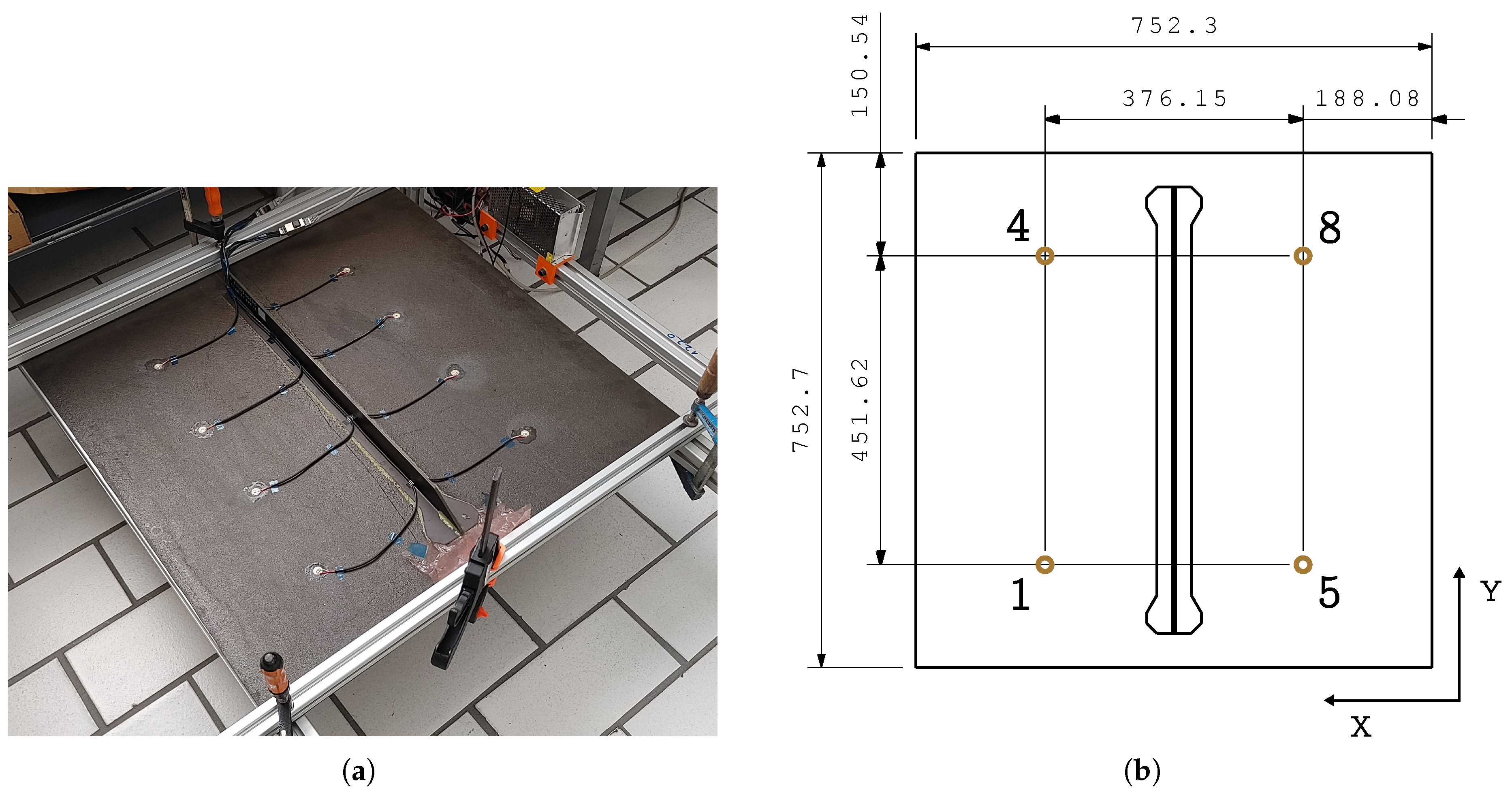
Figure 2.
Autonomous Impactor Machine performing an impact round.
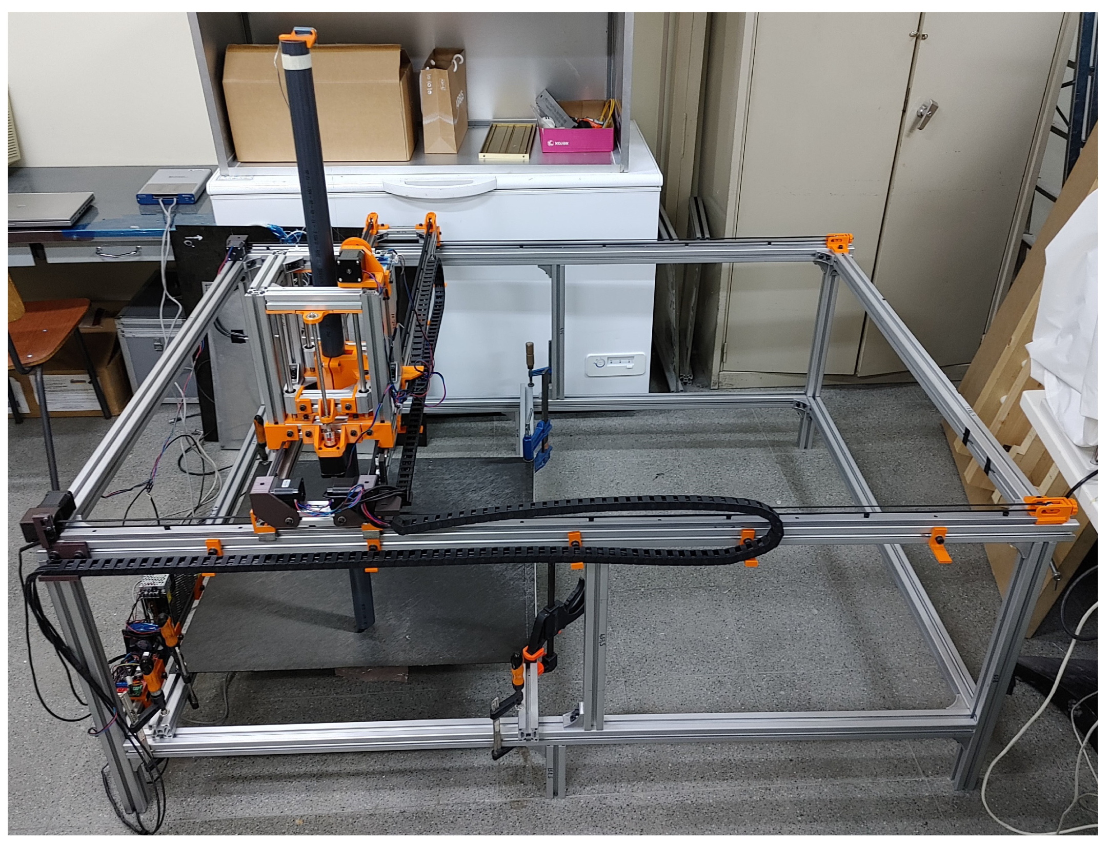
Figure 3.
Coordinate grid of impacts on the specimen and its boundary conditions (aluminum profiles clamp the along-Y edges whereas along-x edges are free)
Figure 3.
Coordinate grid of impacts on the specimen and its boundary conditions (aluminum profiles clamp the along-Y edges whereas along-x edges are free)
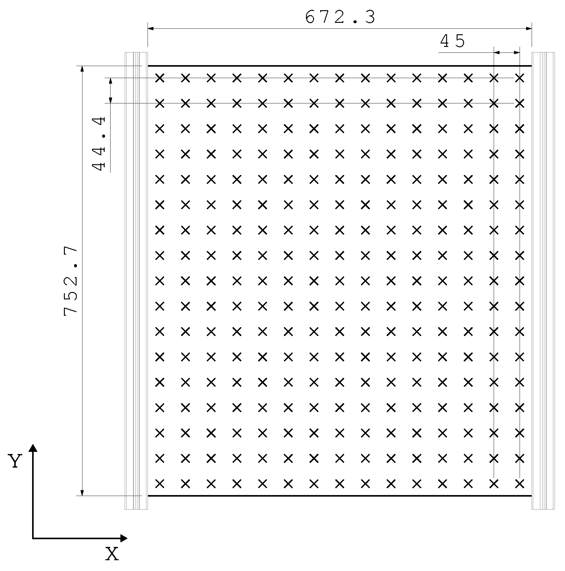
Figure 4.
Diagram of the Deep Neural Network architecture. For more information [1].
Figure 4.
Diagram of the Deep Neural Network architecture. For more information [1].
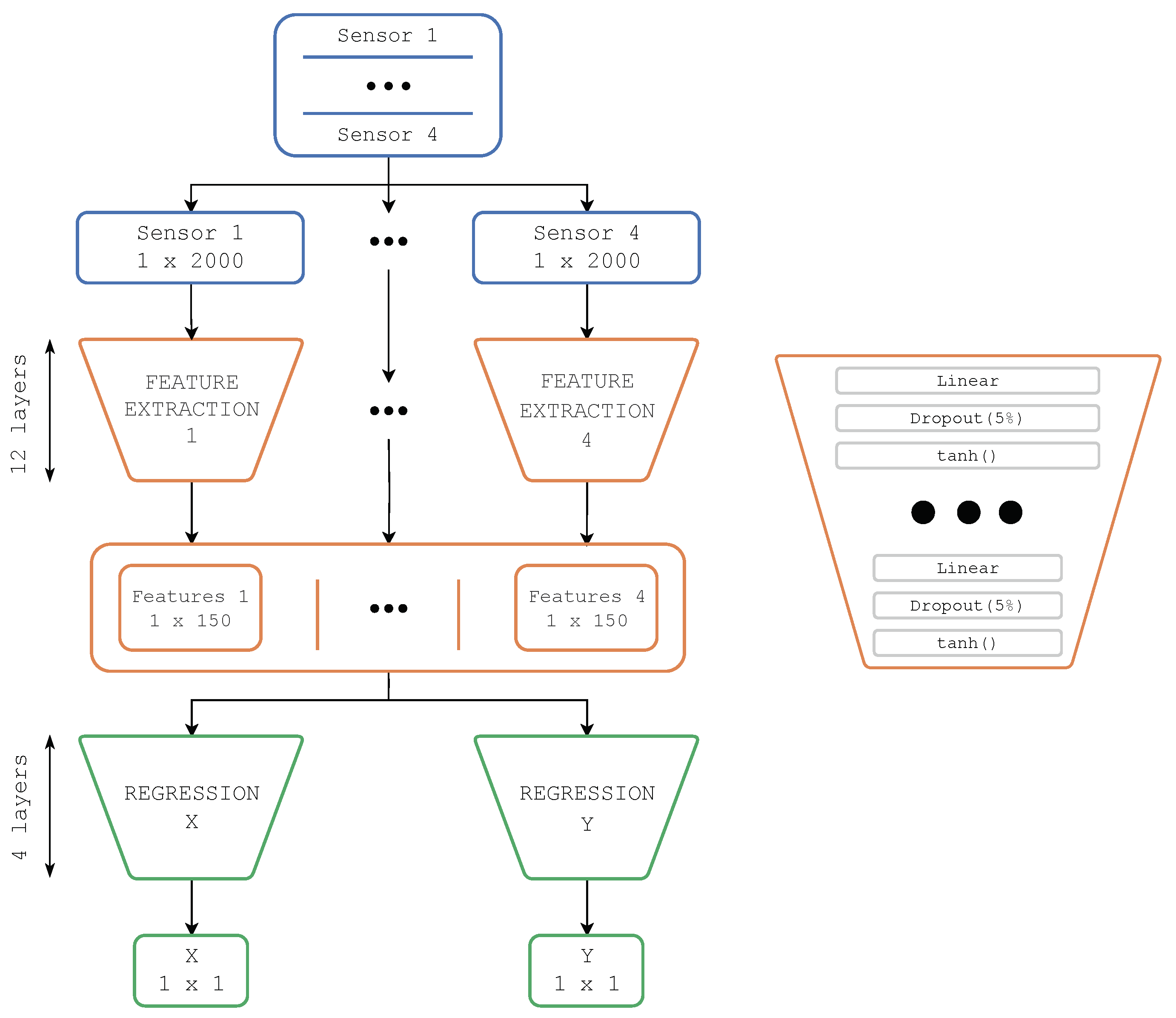
Figure 5.
An example of the training process, demonstrating loss reduction over epochs.
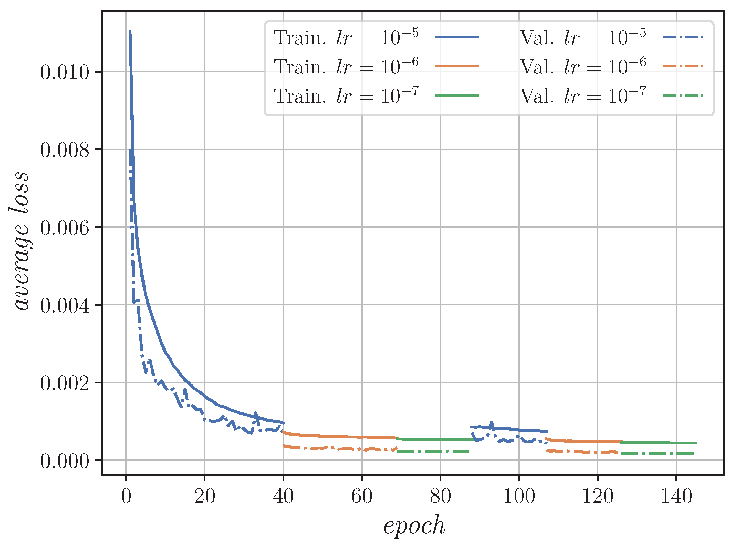
Figure 6.
Time delay perturbation example; Sensor 8 delayed 1.6 ms.
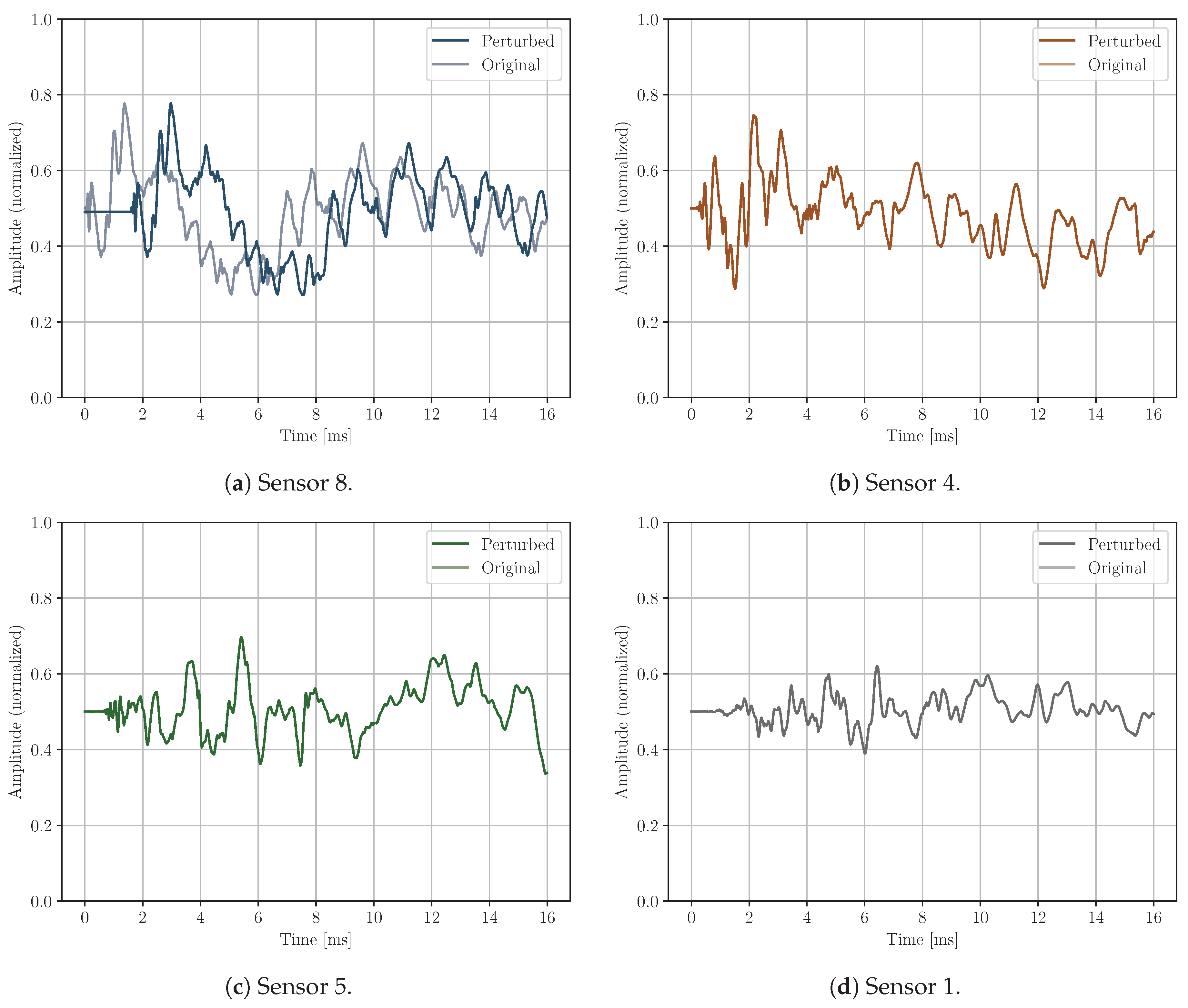
Figure 7.
Sensor cancellation example; Sensor 1 cancelled.
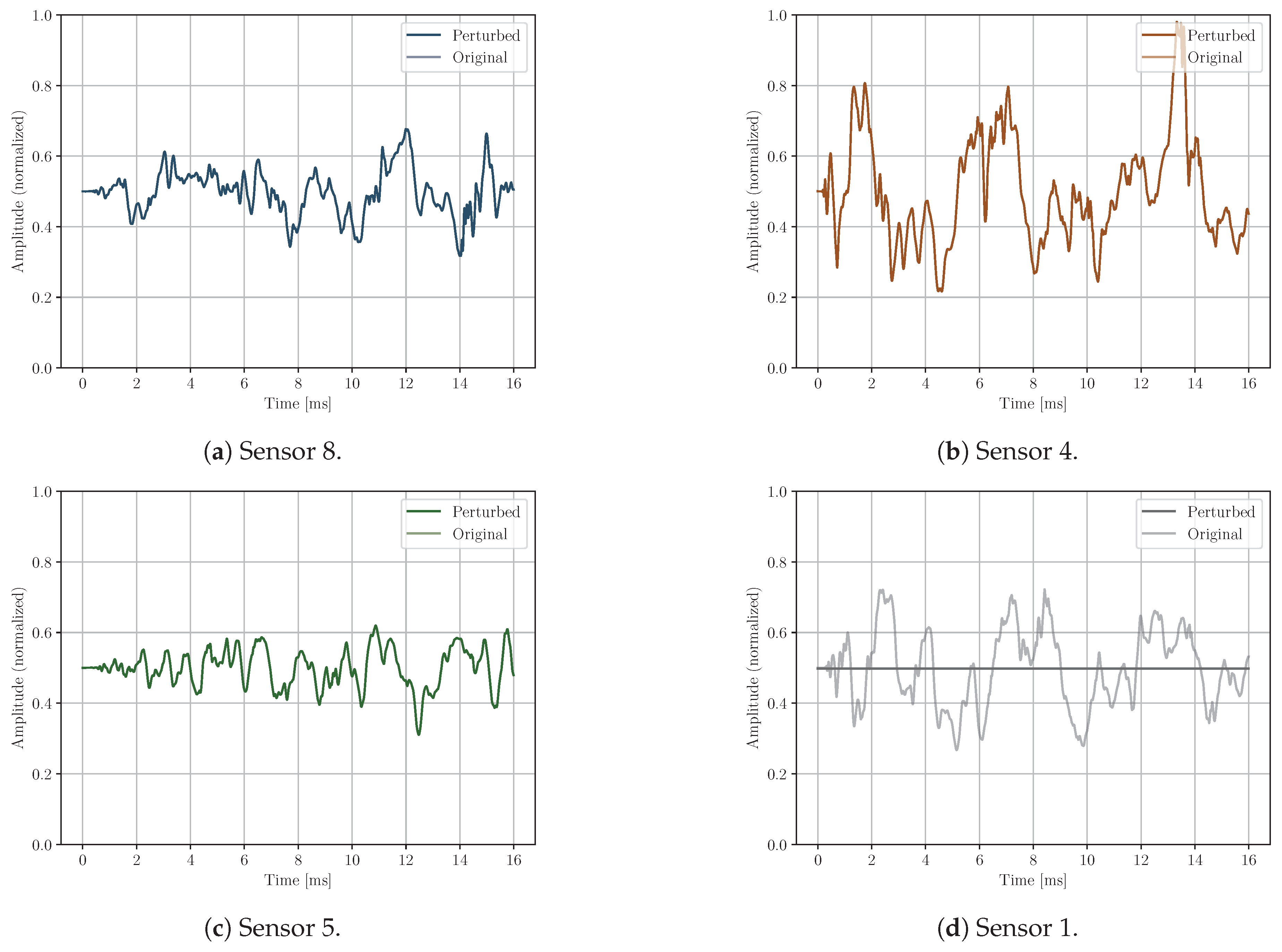
Figure 8.
Noise perturbation example; Sensor 1 affected by noise.
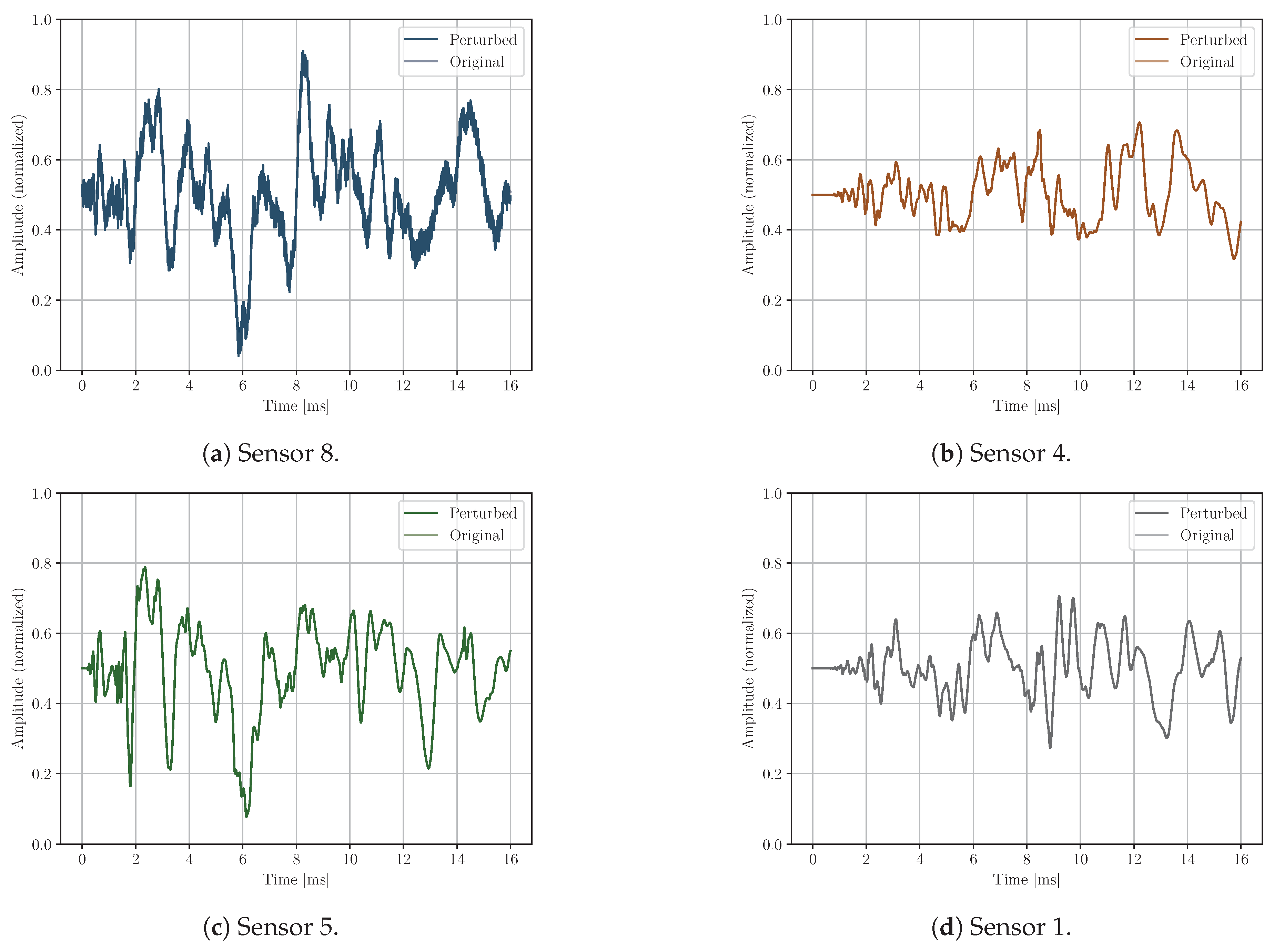
Figure 9.
Noise perturbation example (detail); Sensor 1 affected by noise.
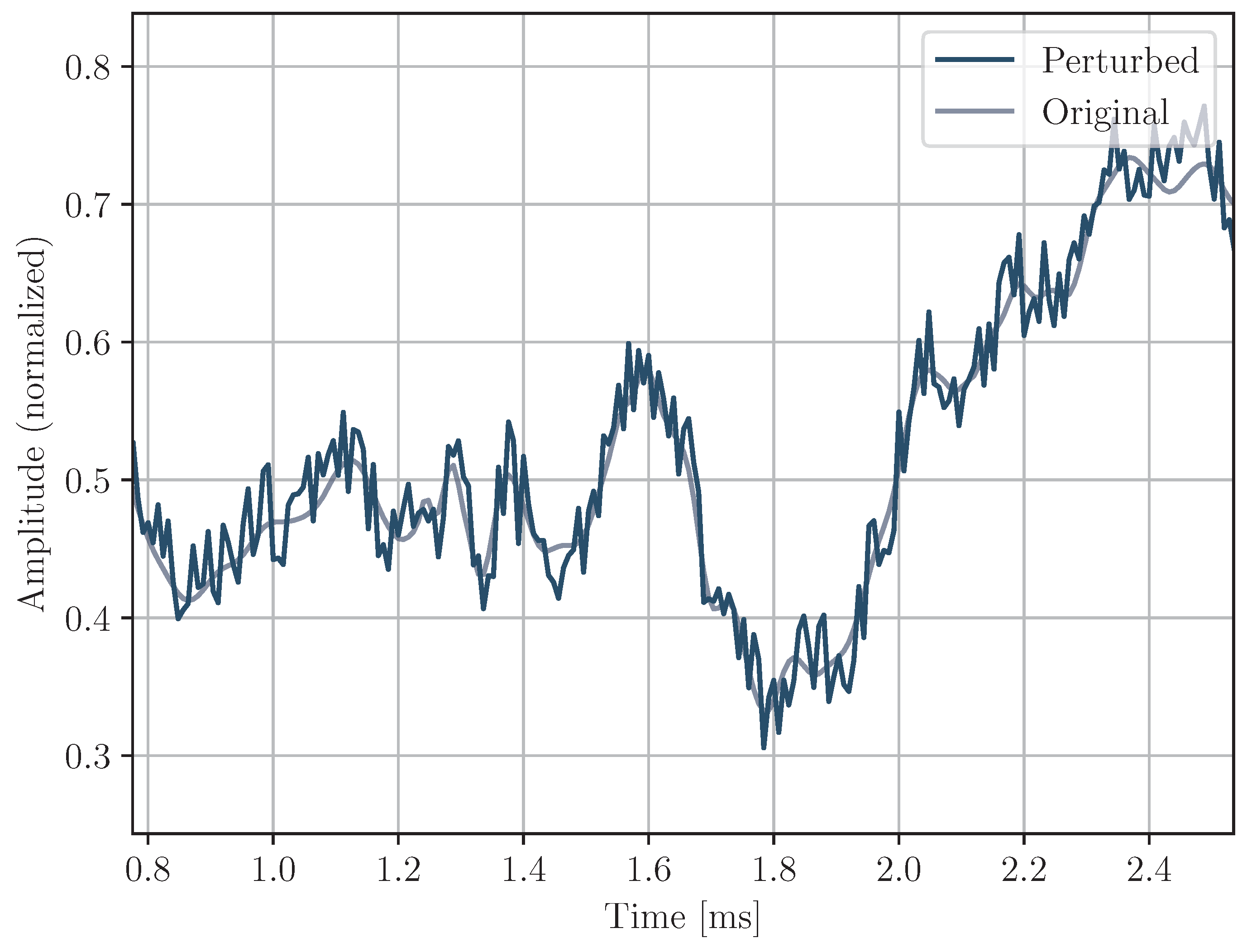
Figure 10.
Predictions from perturbed inputs around the original sample. In this case time delay perturbation method was applied with a range of ± 1.6 ms.
Figure 10.
Predictions from perturbed inputs around the original sample. In this case time delay perturbation method was applied with a range of ± 1.6 ms.
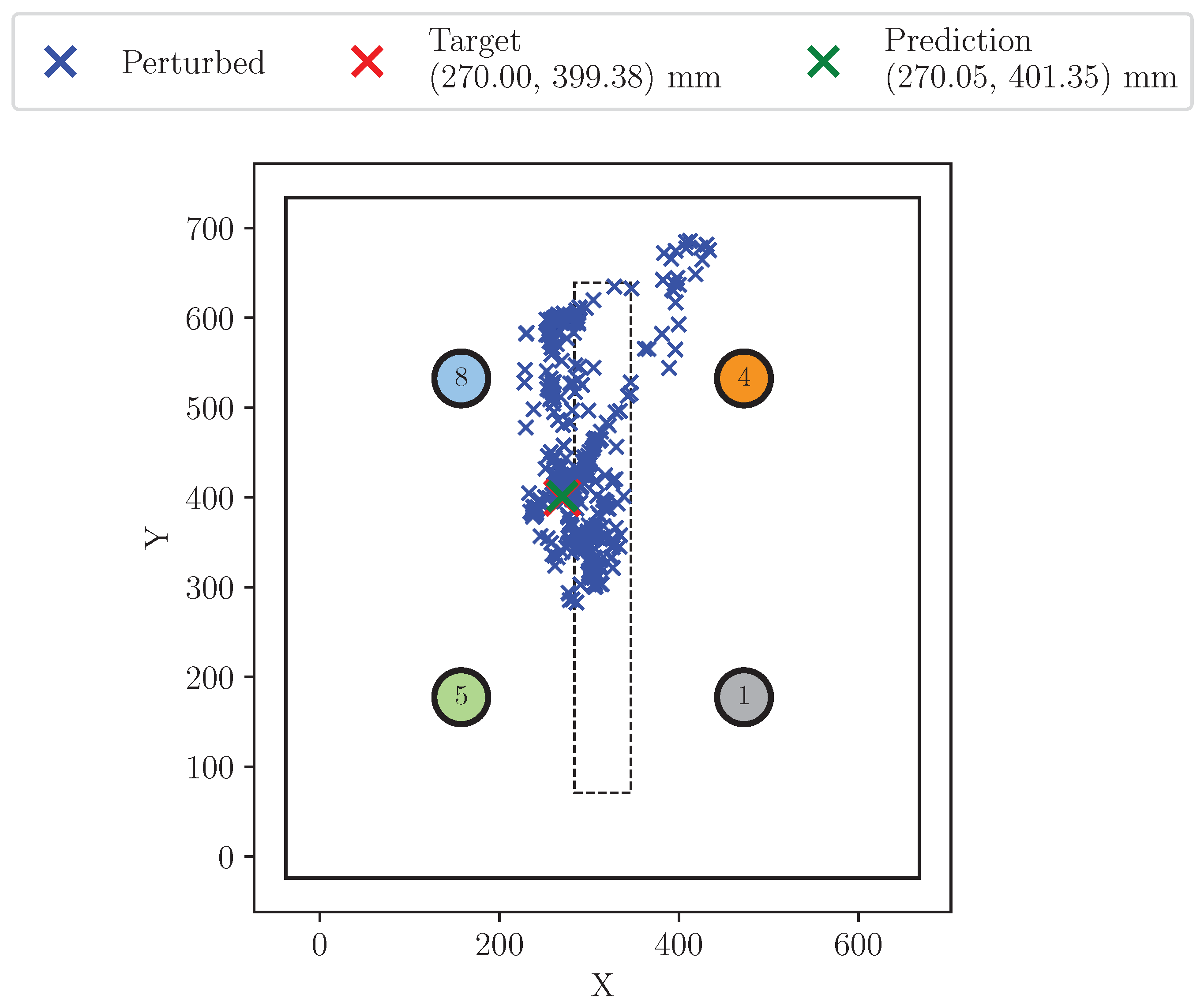
Figure 11.
Example of sensor influence on the prediction of a certain coordinate for an impact performed in certain position by applying a ±1.6 ms time delay perturbation method.
Figure 11.
Example of sensor influence on the prediction of a certain coordinate for an impact performed in certain position by applying a ±1.6 ms time delay perturbation method.
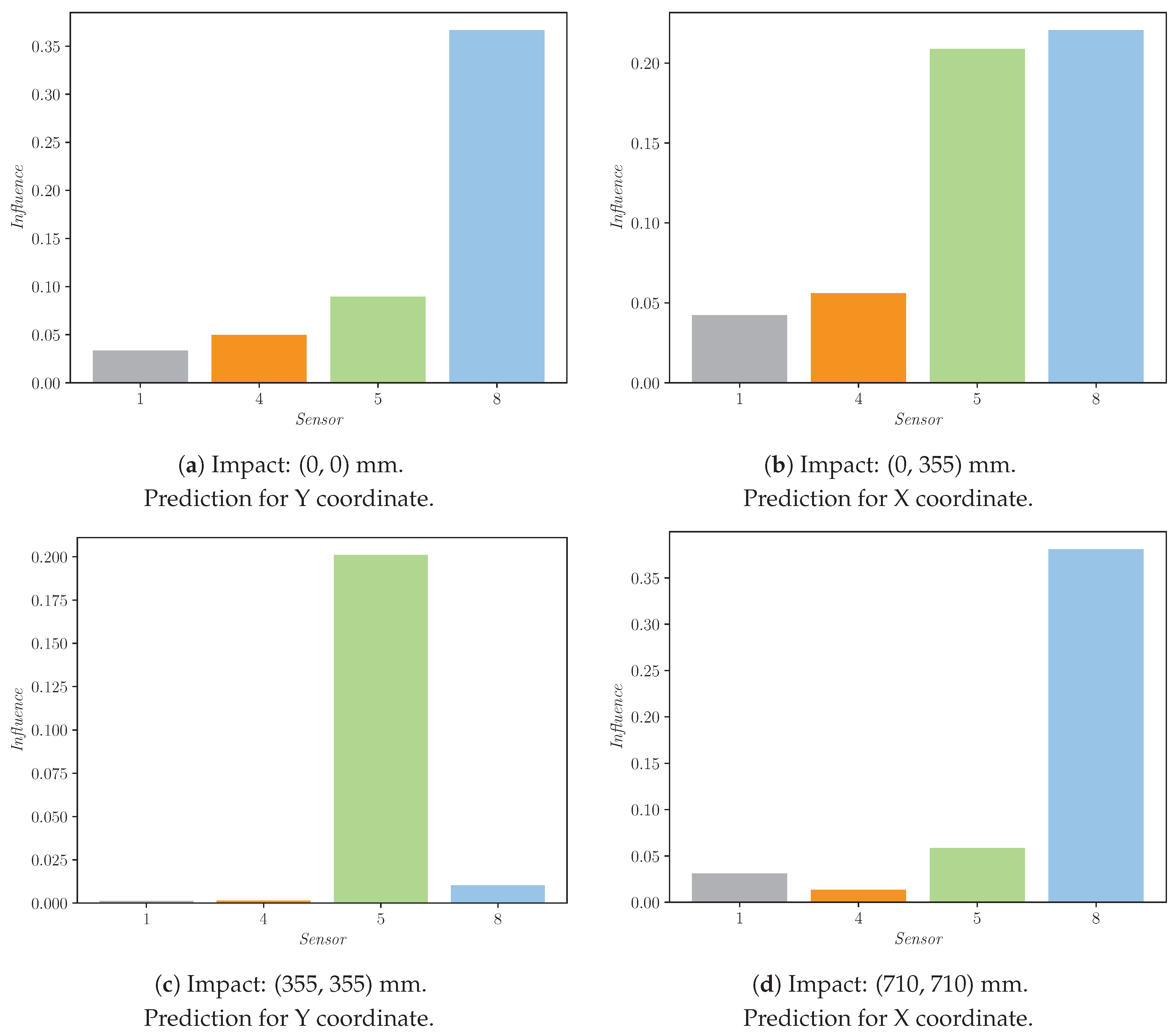
Figure 12.
Mean of sensor perturbation influences on impacts X location prediction all over the plate. Perturbation: time delay in range ms.
Figure 12.
Mean of sensor perturbation influences on impacts X location prediction all over the plate. Perturbation: time delay in range ms.
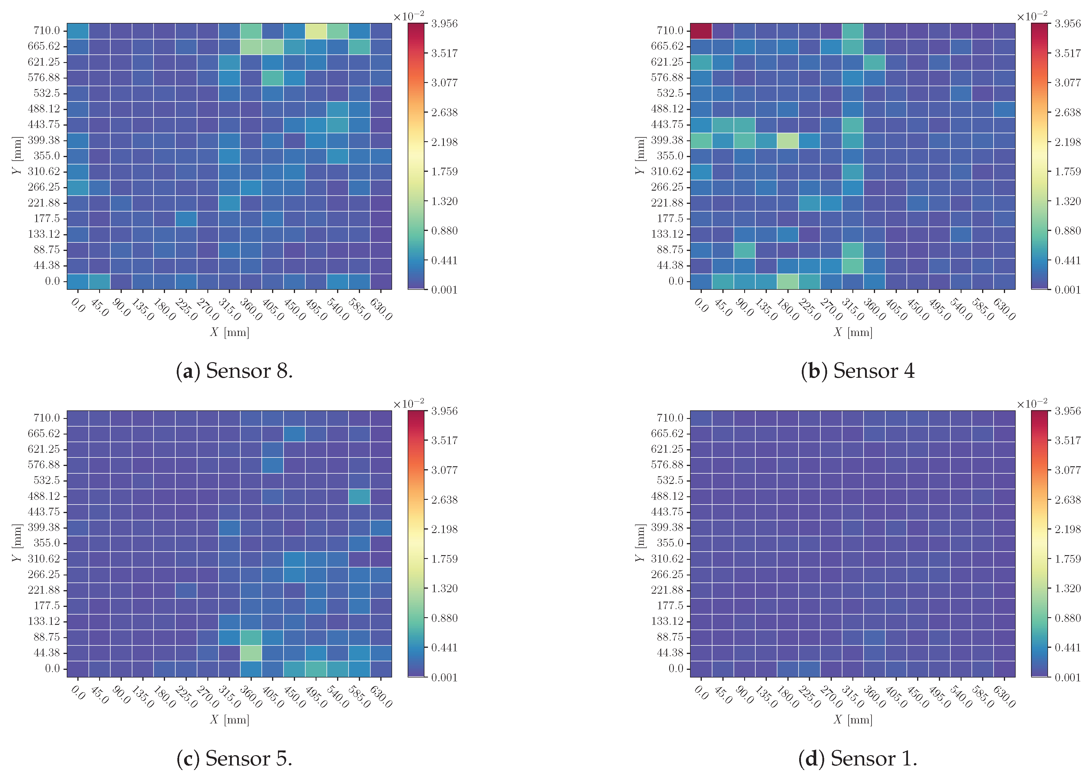
Figure 13.
Mean of sensor perturbation influences on impacts X location prediction all over the plate. Perturbation: time delay in range ms.
Figure 13.
Mean of sensor perturbation influences on impacts X location prediction all over the plate. Perturbation: time delay in range ms.
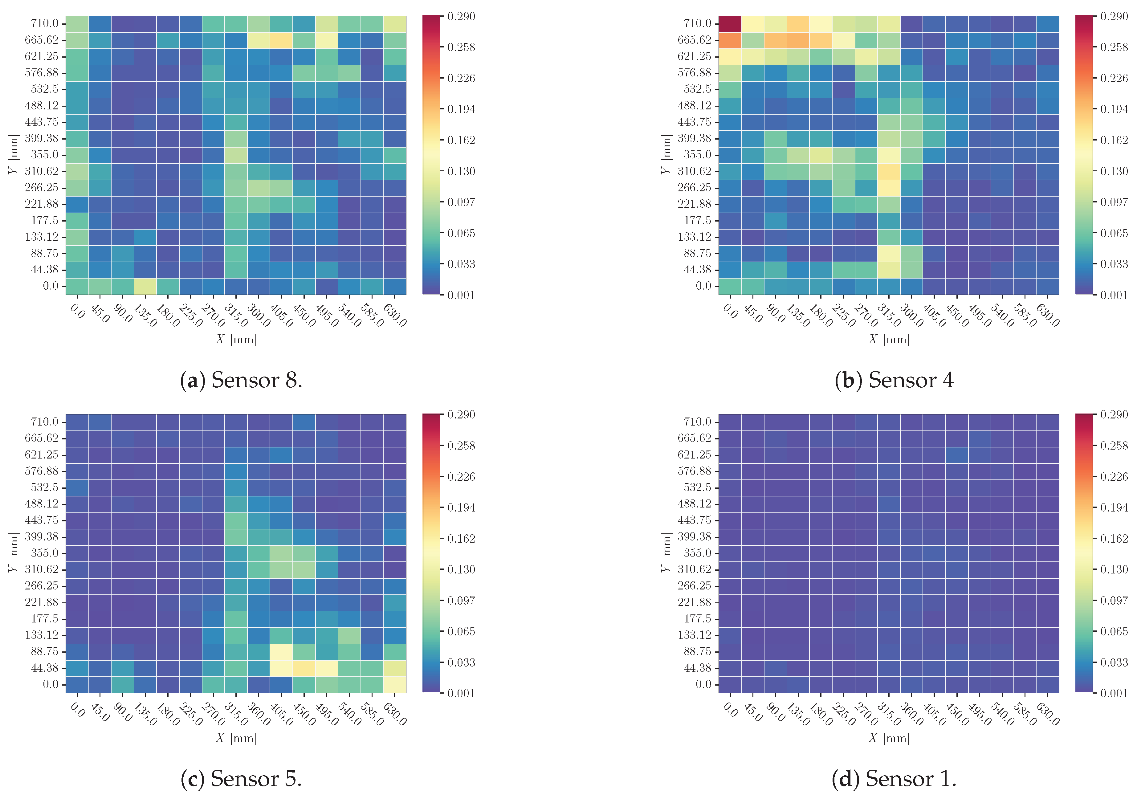
Figure 14.
Mean of sensor perturbation influences on impacts Y location prediction all over the plate. Perturbation: time delay in range ms.
Figure 14.
Mean of sensor perturbation influences on impacts Y location prediction all over the plate. Perturbation: time delay in range ms.
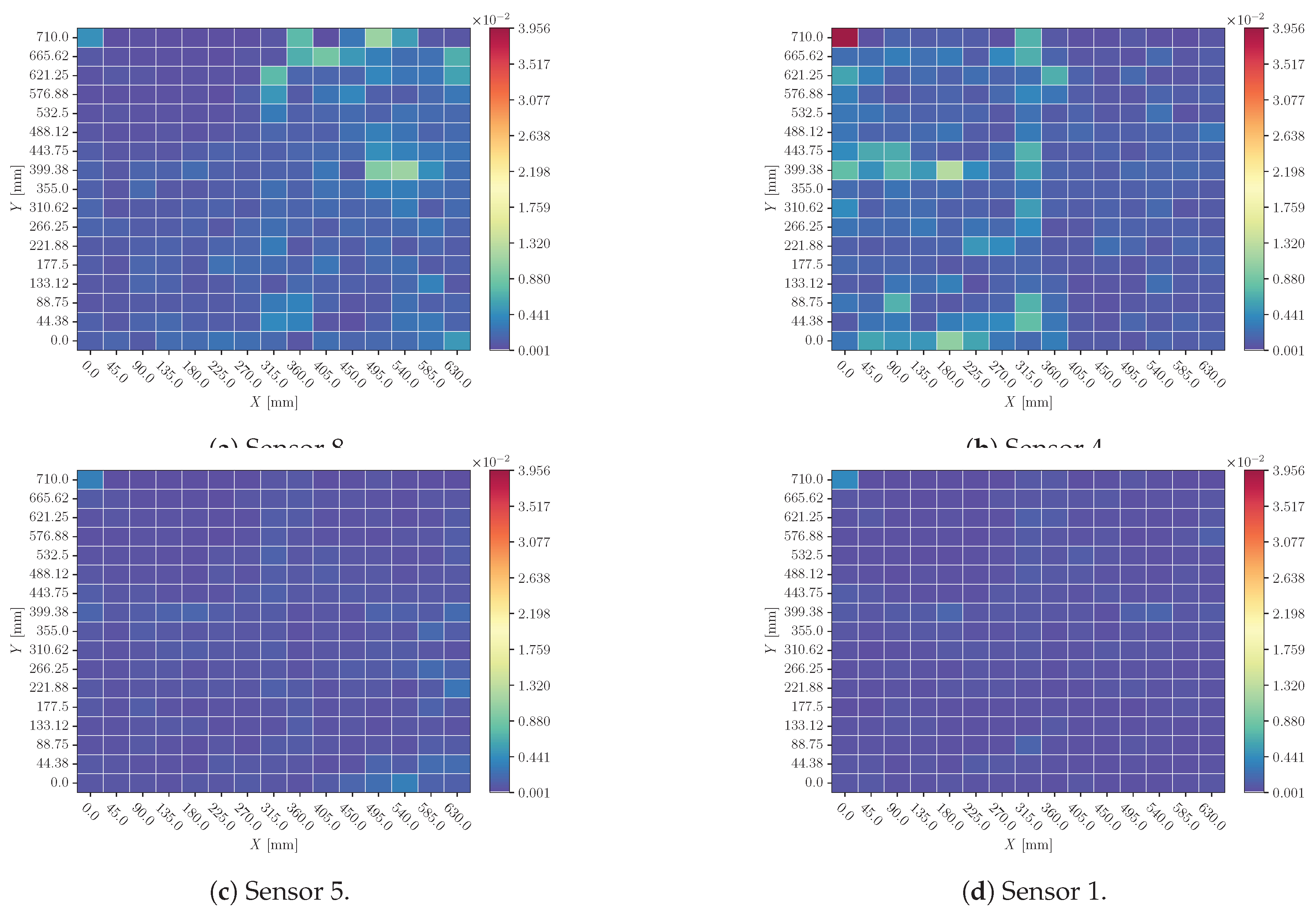
Figure 15.
Mean of sensor perturbation influences on impacts Y location prediction all over the plate. Perturbation: time delay in range ms.
Figure 15.
Mean of sensor perturbation influences on impacts Y location prediction all over the plate. Perturbation: time delay in range ms.
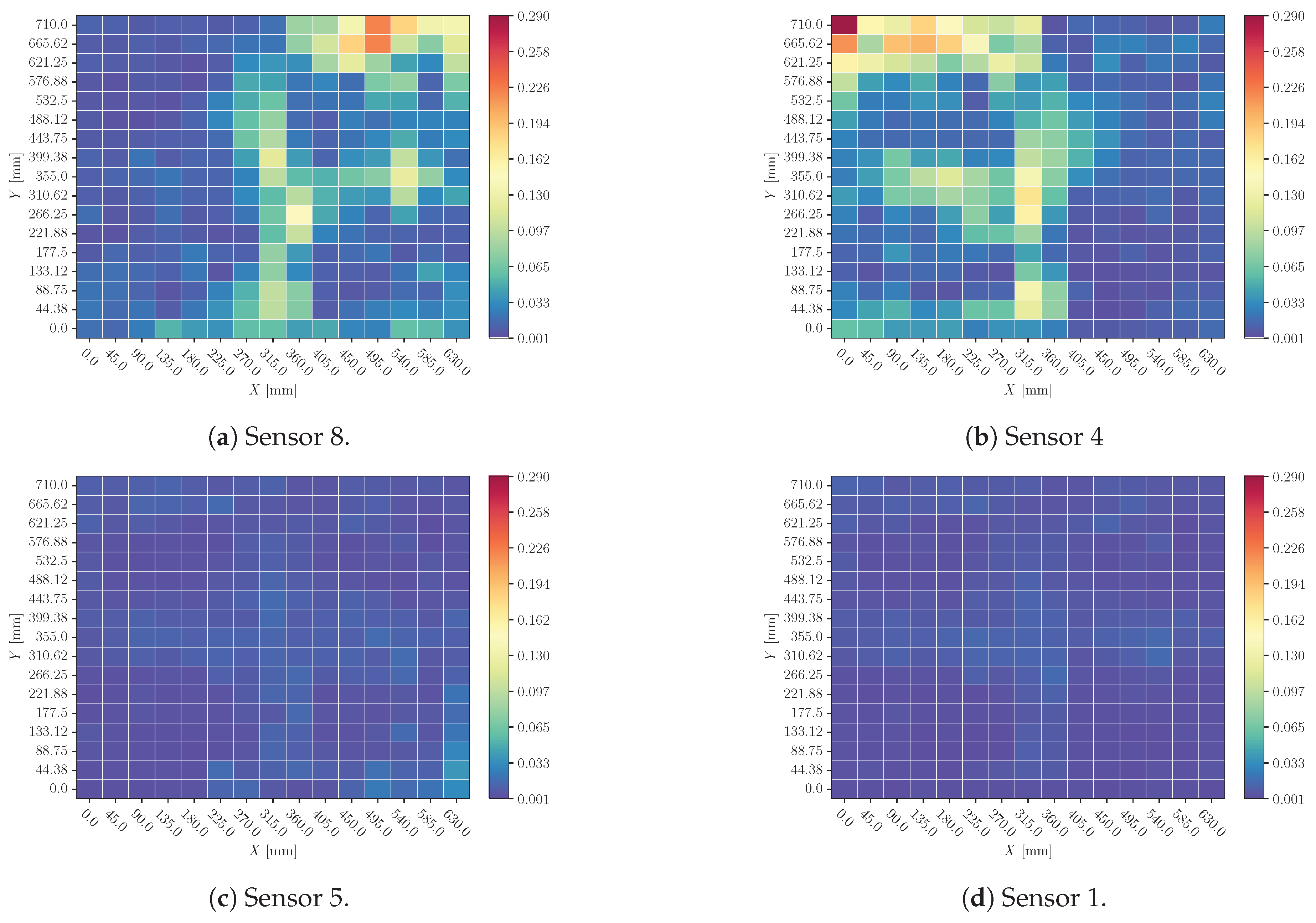
Figure 16.
Mean of sensor perturbation influences on impacts X location prediction all over the plate. Perturbation: sensor cancellation.
Figure 16.
Mean of sensor perturbation influences on impacts X location prediction all over the plate. Perturbation: sensor cancellation.
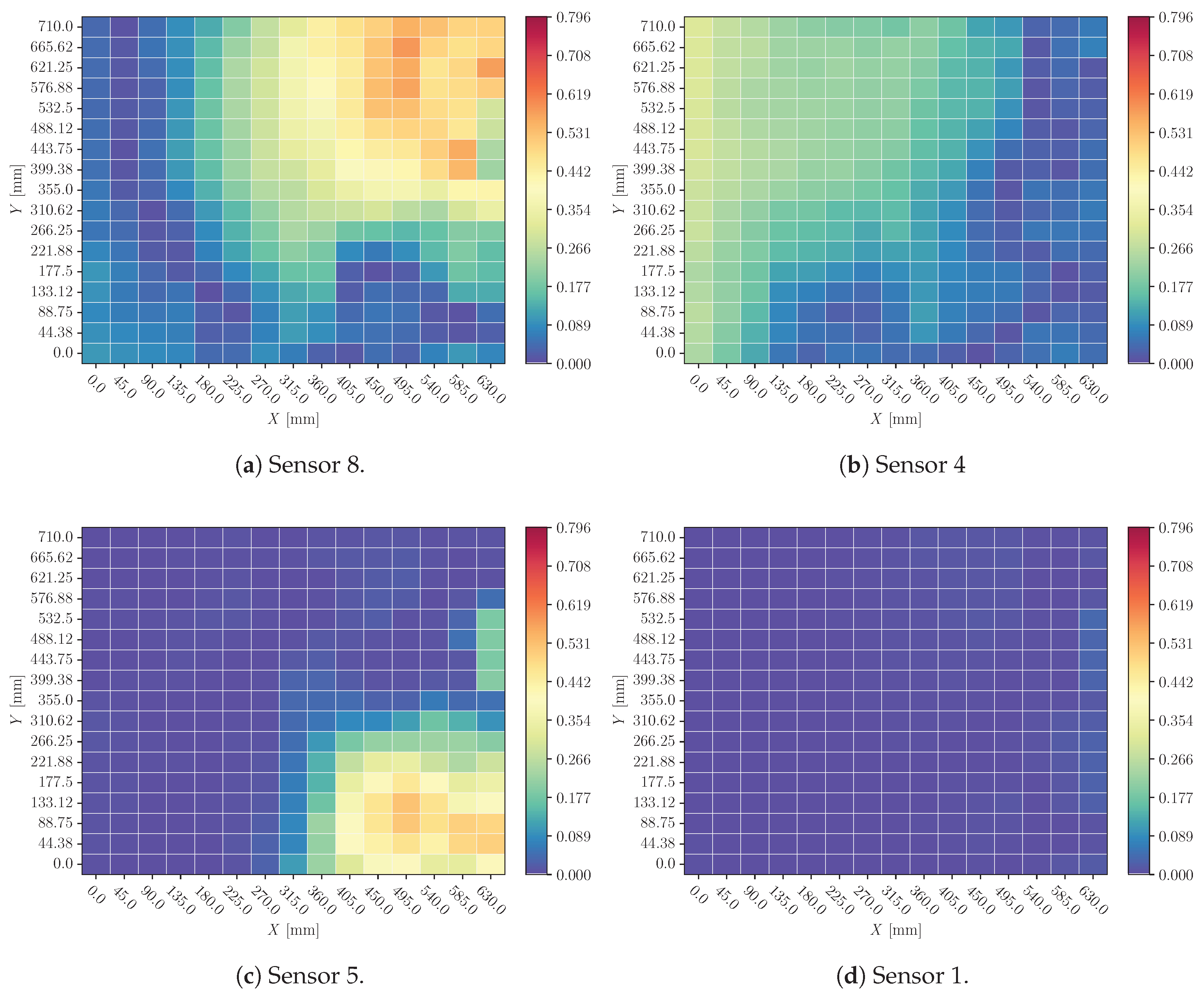
Figure 17.
Standard deviation of sensor perturbation influences on impacts X location prediction all over the plate. Perturbation: sensor cancellation.
Figure 17.
Standard deviation of sensor perturbation influences on impacts X location prediction all over the plate. Perturbation: sensor cancellation.
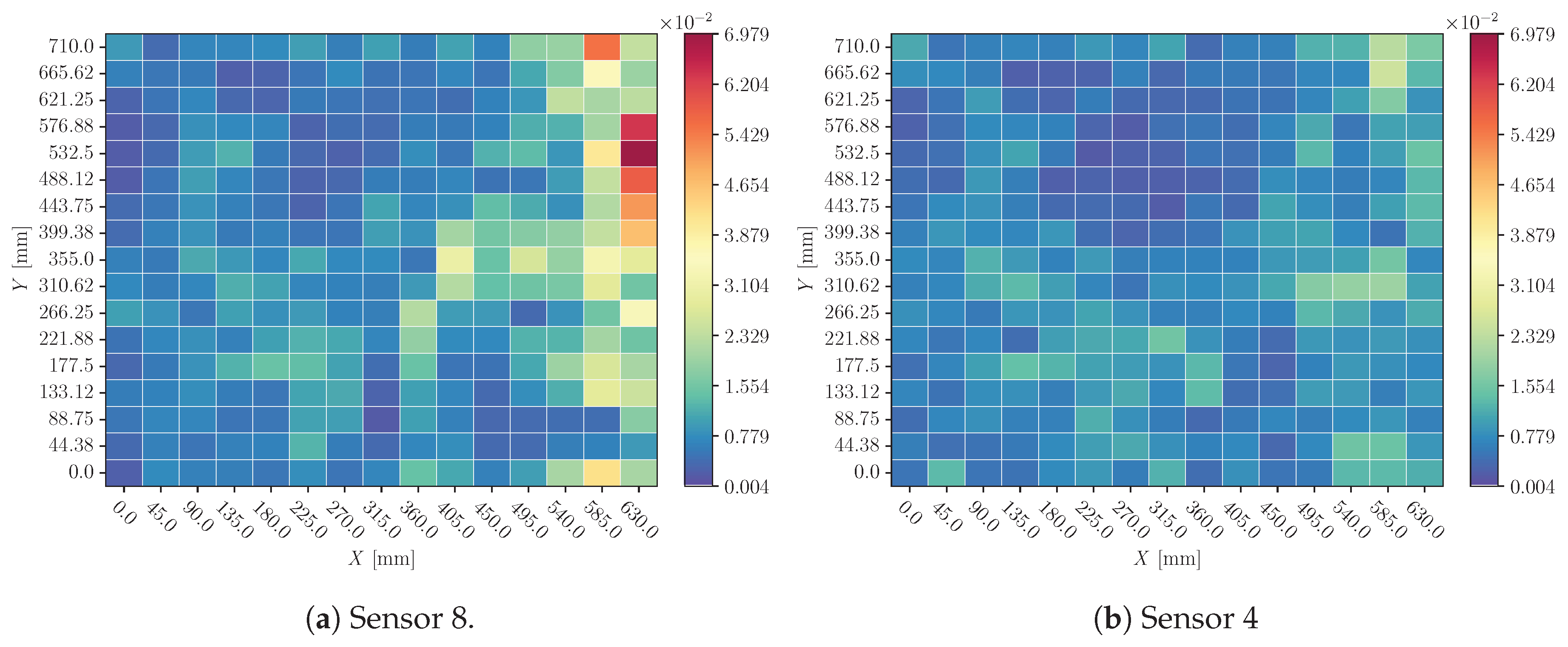
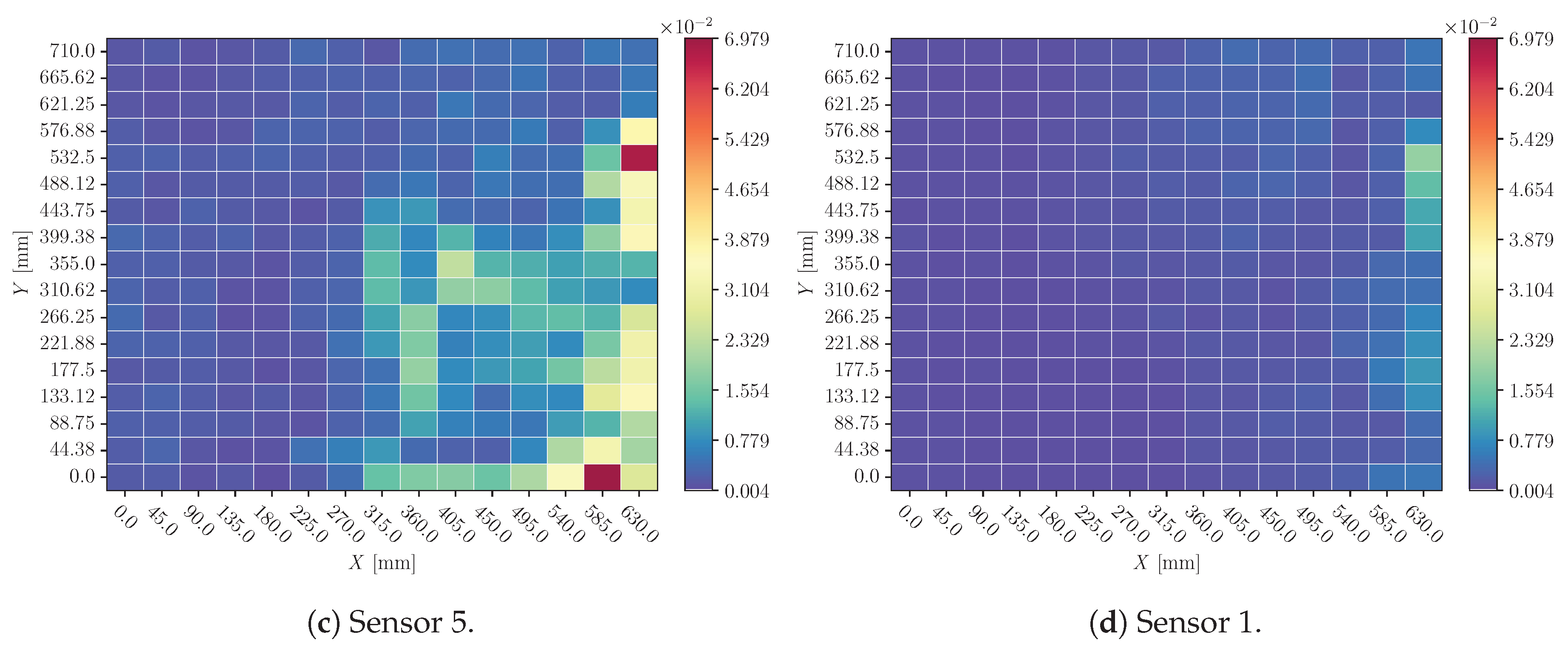
Figure 18.
Mean of sensor perturbation influences on impacts Y location prediction all over the plate. Perturbation: sensor cancellation.
Figure 18.
Mean of sensor perturbation influences on impacts Y location prediction all over the plate. Perturbation: sensor cancellation.
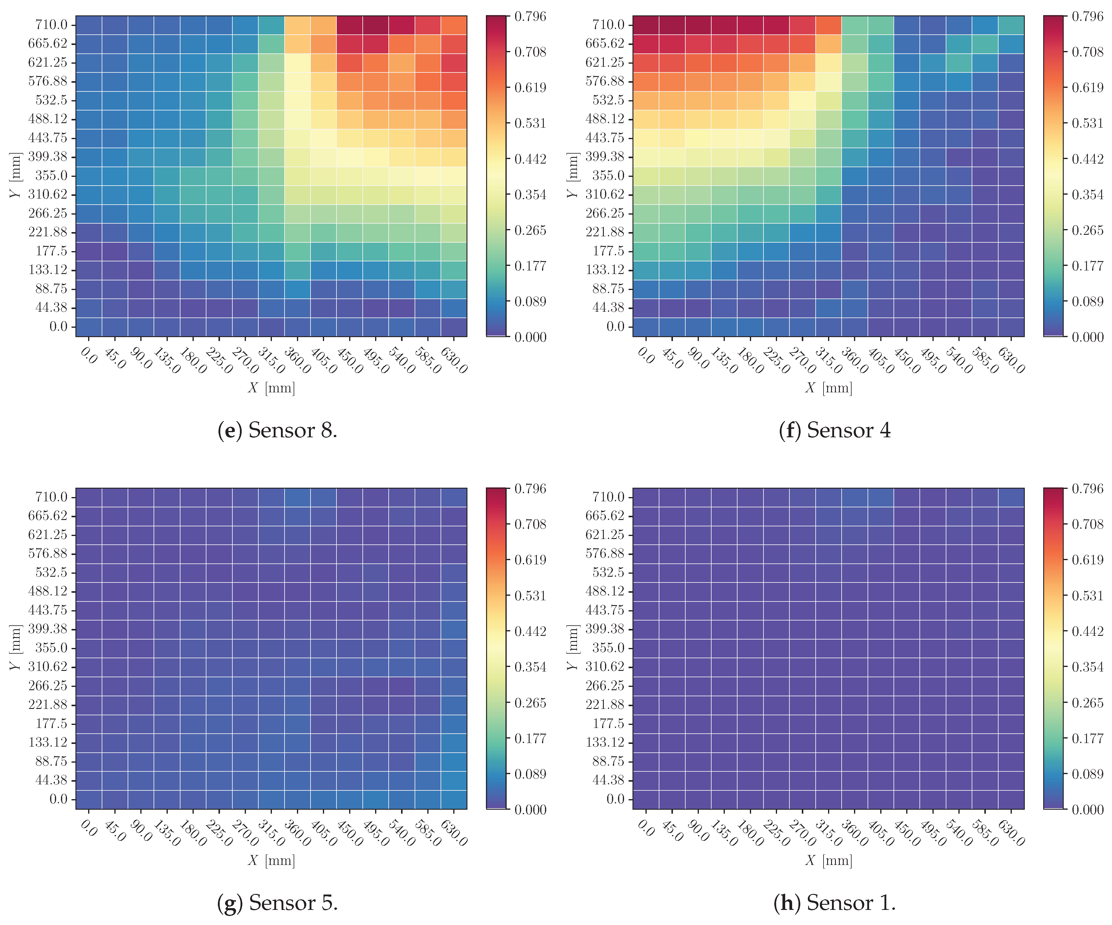
Figure 19.
Standard deviation of sensor perturbation influences on impacts Y location prediction all over the plate. Perturbation: sensor cancellation.
Figure 19.
Standard deviation of sensor perturbation influences on impacts Y location prediction all over the plate. Perturbation: sensor cancellation.
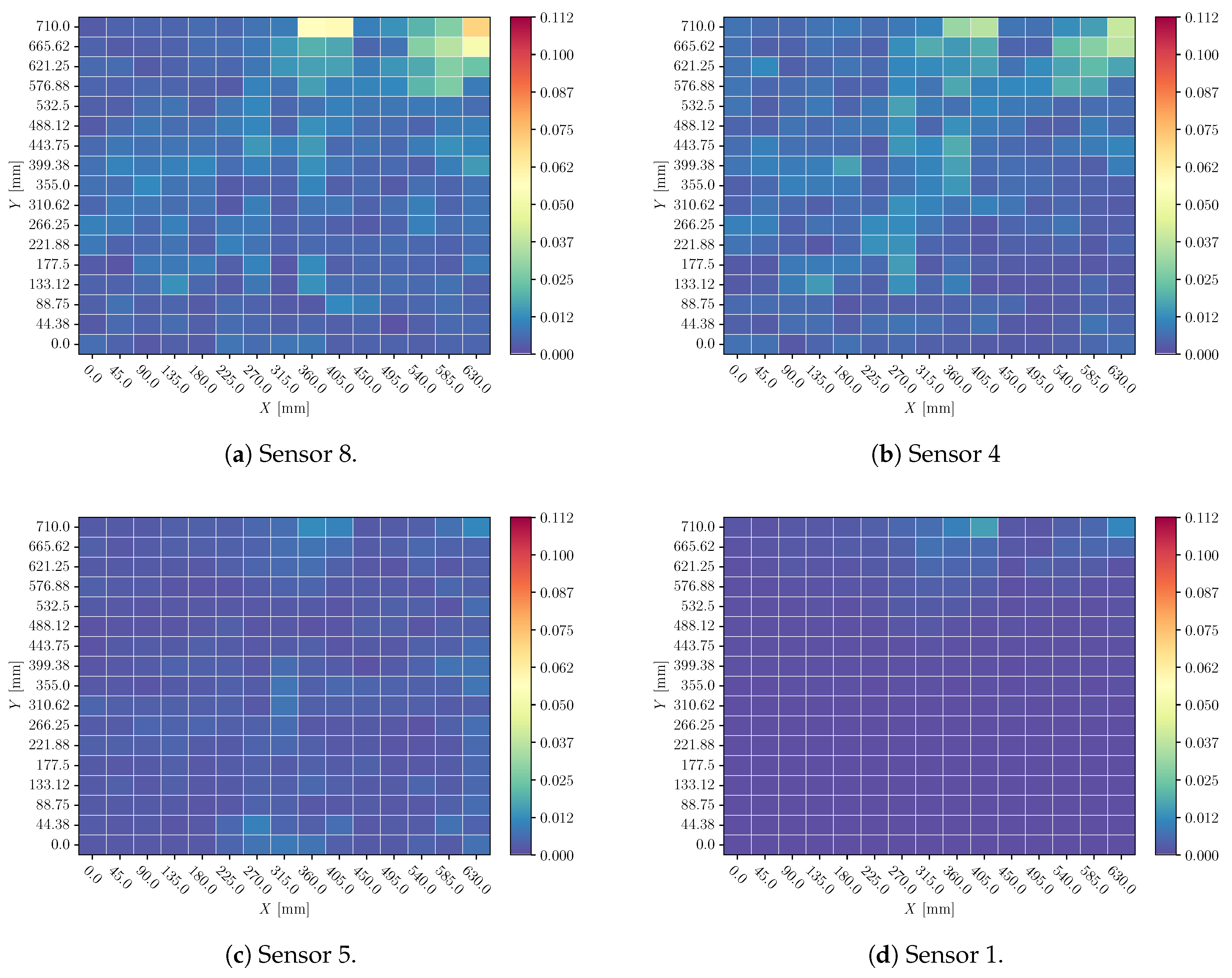
Figure 20.
Mean of sensor perturbation influences on impacts X location prediction all over the plate. Perturbation: white noise with 0.1 SNR.
Figure 20.
Mean of sensor perturbation influences on impacts X location prediction all over the plate. Perturbation: white noise with 0.1 SNR.
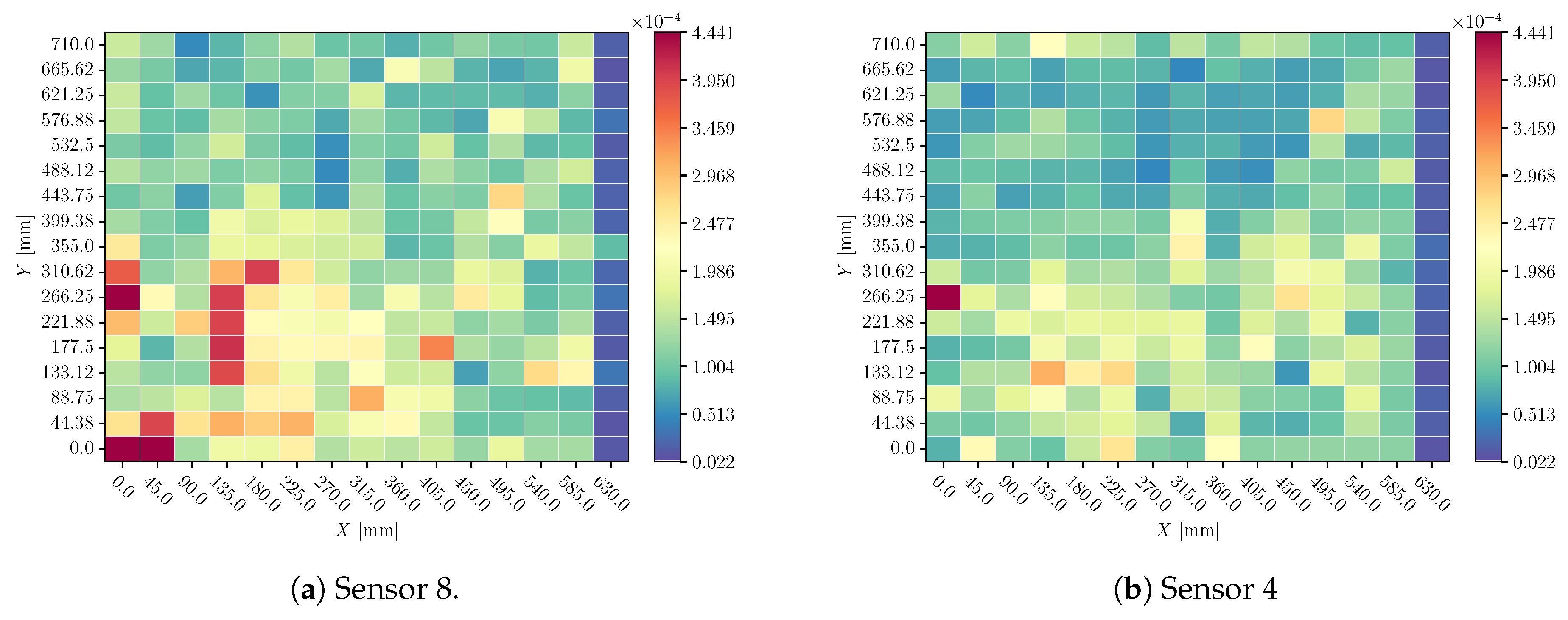
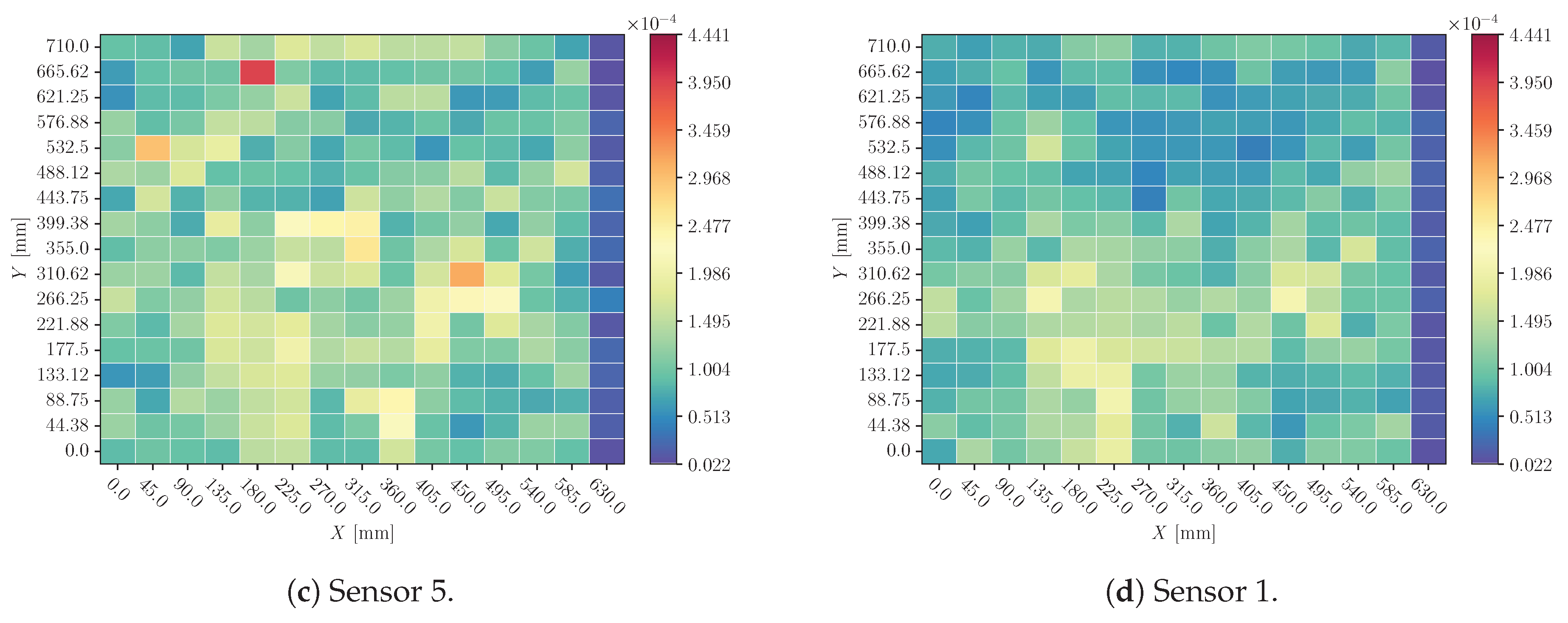
Figure 21.
Mean of ensor perturbation influences on impacts Y location prediction all over the plate. Perturbation: white noise with 0.1 SNR.
Figure 21.
Mean of ensor perturbation influences on impacts Y location prediction all over the plate. Perturbation: white noise with 0.1 SNR.
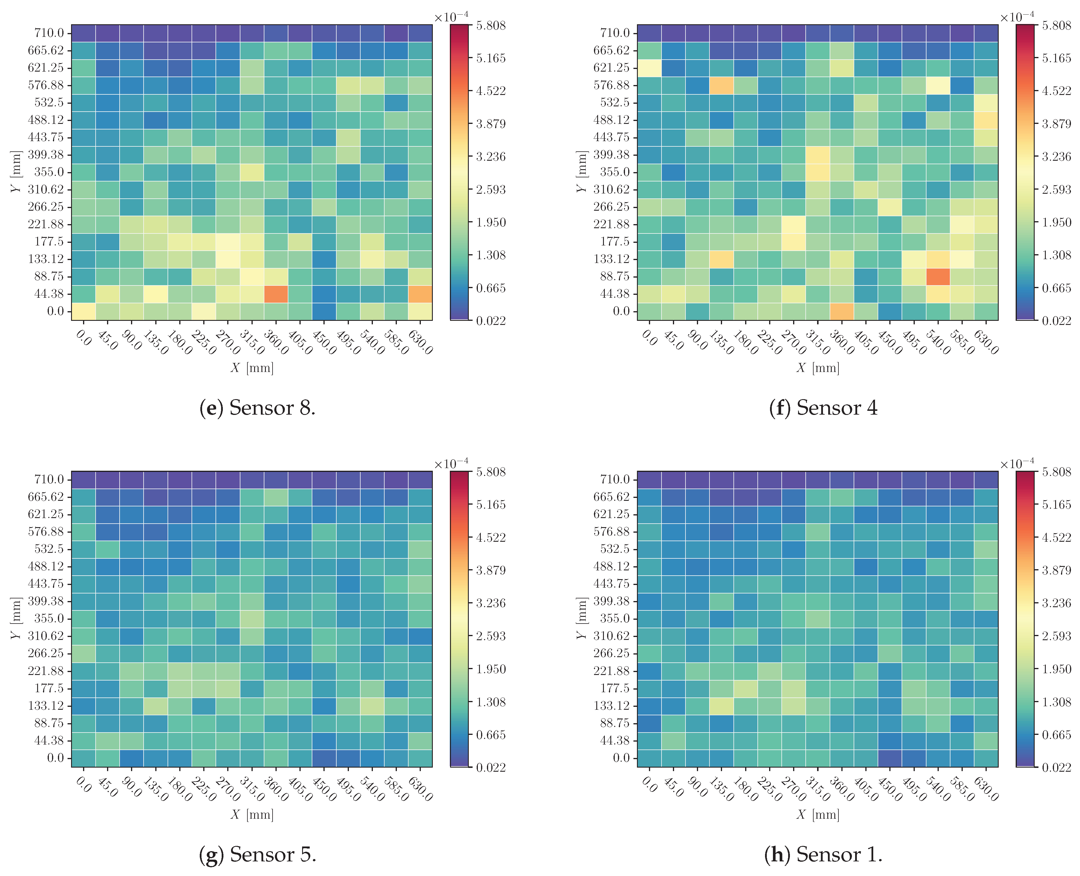

Table 1.
Performance metrics for the trained models. For more information [1].
Table 1.
Performance metrics for the trained models. For more information [1].
| Model [k] | [mm] | [mm] |
|---|---|---|
| 1 | 3.54 | 2.29 |
| 2 | 3.37 | 2.29 |
| 3 | 3.50 | 2.25 |
| 4 | 3.47 | 2.38 |
| Average | 3.47 | 2.30 |
Disclaimer/Publisher’s Note: The statements, opinions and data contained in all publications are solely those of the individual author(s) and contributor(s) and not of MDPI and/or the editor(s). MDPI and/or the editor(s) disclaim responsibility for any injury to people or property resulting from any ideas, methods, instructions or products referred to in the content. |
© 2025 by the authors. Licensee MDPI, Basel, Switzerland. This article is an open access article distributed under the terms and conditions of the Creative Commons Attribution (CC BY) license (https://creativecommons.org/licenses/by/4.0/).
Copyright: This open access article is published under a Creative Commons CC BY 4.0 license, which permit the free download, distribution, and reuse, provided that the author and preprint are cited in any reuse.


