
Submitted:
01 April 2025
Posted:
03 April 2025
You are already at the latest version
Abstract
This survey provides a review of the theoretical research on the classic system of matrix equations AX = C and XB = D, which has wide-ranging applications across fields such as control theory, optimization, image processing, and robotics. The paper discusses various solution methods for the system, focusing on specialized approaches, including generalized inverse methods, matrix decomposition techniques, and solutions in the forms of Hermitian, extreme rank, reflexive, and conjugate solutions. Additionally, specialized solving methods for specific algebraic structures, such as Hilbert spaces, Hilbert C∗-modules, and quaternions, are presented. The paper explores the existence conditions and explicit expressions for these solutions, along with examples of their application in electronic network and color image.
Keywords:
system of matrix equations
; general solution
; special solution
; Moore-Penrose inverse
; matrix decomposition
1. Introduction
Systems of equations, particularly
are essential tools in linear algebra and have widespread applications in diverse scientific and engineering disciplines. These equations often appear in various domains such as control theory, optimization, image processing, system identification, and robotics [1,2,3,4,5,6,7]. Specifically, the matrix system can represent the state-space model of a dynamic system, where A and B correspond to system transformations, X represents the system state, and C and D are the output matrices [8]. Solving these equations provides the system’s state at a given time. In signal processing, particularly in filter design and signal reconstruction, the filter matrix X transforms input signals A to output C, ensuring the transformed signal interacts correctly with B to produce output D[9]. This concept extends to image processing, where matrices A and B represent operations (e.g., encryption), and C and D are the original and transformed images. Solving for X gives the required transformation. In robotics and computer vision, this matrix system arises in rigid body transformations. Dual quaternions represent 3D transformations, where A and B may represent rotation and translation, and X is the transformation matrix [10]. This system is vital for solving inverse kinematics problems, such as determining joint parameters of a robotic arm.
This paper aims to summarize the theoretical results related to the matrix equation system (1), mainly focusing on the conditions and corresponding expressions for the existence of general solutions, least squares solutions, and minimum norm solutions. The paper also highlights generalized inverse methods and matrix decomposition methods in real and complex fields, as well as special solving methods for certain algebraic structures, such as Hilbert - modules, Hilbert spaces, rings, dual numbers, quaternions, split quaternions, and dual quaternions.
The most widely used and earliest approach for solving system (1) is based on generalized inverses or inner inverses. For special forms of solutions, such as Hermitian, nonnegative definite, maximal and minimal rank solutions, and generalized (anti-)reflexive solutions, this class of methods provides a rich theoretical framework. On the other hand, matrix decomposition is a powerful tool for solving more complex special forms of solutions. Due to the different forms resulting from various matrix decompositions, these special forms can be used to construct corresponding special solutions. Related research covers symmetric, mirror-symmetric, bi-(skew-)symmetric, and orthogonal solutions over the real numbers, as well as unitary, (semi-)positive definite, generalized reflexive, generalized conjugate, and Hamiltonian solutions over the complex numbers.
For certain special algebraic structures, there are specialized solving methods. For example, in Hilbert -modules, Hilbert spaces, and rings, inner inverses are widely used. For quaternions, dual numbers, and dual quaternions, generalized inverses can also be applied to solve the system (1). However, in the case of split quaternions, matrix representations are the more widely used approach for solving the system. Additionally, some researchers have discussed the use of determinants to express the form of solutions for quaternion systems. This paper also provides examples of applying the system (1) to dual quaternion matrices and dual split quaternion tensors for the encryption and decryption of color images and videos.
The remainder of the paper is organized as follows. Chapter 2 introduces generalized inverse methods for solving the general solution, Hermitian and nonnegative definite solutions, maximal and minimal rank solutions, and generalized reflexive solutions. The study of system (1) in Hilbert -modules, Hilbert spaces, and rings is presented in Chapter 3. Chapter 4 discusses eigenvalue decomposition, singular value decomposition, and generalized singular value decomposition of matrices, along with research conclusions for some special solutions of system (1). Chapters 5 and 6 focus on the studies of dual numbers and quaternions, respectively. Chapter 7 introduces examples of using the system (1) in the encryption and decryption of color images and videos. Finally, Chapter 8 summarizes the content of the paper.
For convenience in the narration of this paper, the following notations are used uniformly. Symbols , , , and represent the real number field, the complex number field, the set of matrices over the real numbers, the set of complex vectors with n elements, and the set of matrices over the complex numbers, respectively. O and I denote appropriately sized zero matrices and identity matrices. For an arbitrary matrix A, , and represent the conjugate, transpose and conjugate transpose of A, respectively. For an matrix A over the real numbers, complex numbers, or quaternions, represents the rank of A and expresses the range (column space) of A. For a complex square matrix A, it is (semi-)positive definite if and only if for every , we have . For two complex square matrices A and B of the same size, we say that in the Löwner partial ordering if is (semi-)positive definite. The symbols and denote the numbers of positive and negative eigenvalues of a Hermitian complex matrix A, counted with multiplicities. Note that for Hermitian nonnegative definite matrix A, denote is the matrix satisfying . The mentioned below all represents the Frobenius-norm of a matrix.
2. The Generalized Inverse Methods for Solving (1)
Since 1954, Penrose has described a generalization of the inverse of non-singular matrices through the unique solution of a system of four matrix equations [11]. This area has since attracted considerable attention.
For , there exists a unique satisfying the following system:
where is called the general inverse or the Moore-Penrose inverse of A. In the following discussion, we denote the symbols and .
Penrose proposed the necessary and sufficient conditions for the matrix system , along with an expression for its solutions in terms of the general inverse.
Theorem 1
(General solutions using the Moore-Penrose inverse for (1) over ). [11] Let . The matrix system (1) is solvable if and only if the equations and are consistent, and the condition holds, or equivalently,
Under these conditions, the general solution is given by
Remark 1.
Later, the concept of the g-inverse of a complex matrix was introduced by Rao and Mitra [13]. For , if the matrix satisfies
then is defined as the g-inverse of A.
Remark 2.
The g-inverse of a complex matrix is not necessarily unique.
The g-inverse can also be used to represent the solution of linear matrix systems. Theorem 1 can be restated in terms of the g-inverse as follows.
Theorem 2
(General solutions using the g-inverse for (1) over ). [16] Let . The matrix system (1) is solvable if and only if
When (1) is consistent, the general solution is expressed as
where is arbitrary.
Subsequently, researchers have investigated a series of special solutions to system (1) using generalized inverses, including Hermitian solutions, nonnegative solutions, maximal and minimal rank solutions, general (anti-)reflexive solutions, real nonnegative or real positive solutions, and others.
The earliest research on the Hermitian and nonnegative definite solutions of system (1) was conducted by Mitra et al. [14], followed by their subsequent work on the possible minimal rank of the solutions [15]. Mitra’s focus on matrix equation systems continued, and in 1990, he extended the study to a more general form of the system [16]. After 2000, research on system (1) became more in-depth: Peng and other scholars investigated the (anti-)reflexive solutions of the system [17,18,19,20,21,22,23], while Liu et al. focused on the least squares solutions and the rank of the solutions, exploring the ranks of matrix blocks and the corresponding conditions using block matrix formulations [24,25]. Due to the unique properties of Hermitian matrices, Wang et al. examined the existence conditions and expressions for Hermitian solutions to system (1) that satisfy various inequality constraints, as well as the ranks and inertia indices of these solutions [26,27,28]. Additionally, some scholars have focused on bi-(skew-)symmetric solutions and reducible solutions [29,30].
2.1. Hermitian, Nonnegative Solutions
Hermitian and nonnegative matrices are among the most widely applied special types of matrices, and their associated properties have been thoroughly studied. A complex square matrix is called Hermitian if .
In 1976, Khatri and Mitra considered the necessary and sufficient conditions for the existence of Hermitian and nonnegative definite solutions to system (1), and provided expressions for the solutions when they exist. The main results are stated in Theorem 3.
Theorem 3
(Hermitian and nonnegative solutions for (1) over ). [14] Let and such that the system (1) is solvable. Define
The system (1) has Hermitian solutions if and only if M is Hermitian. Under this condition, a general Hermitian solution is given by
where is an arbitrary Hermitian matrix.
The system (1) has nonnegative definite solutions if and only if M is nonnegative definite and . Under this condition, general nonnegative definite solutions have the form of
where is an arbitrary nonnegative definite matrix.
Based on Theorem 3, the following theorem considers the solvability conditions and explicit expressions for the Hermitian solutions to the system (1) with inequality constraints:
and
for given and Hermitian .
Theorem 4
(Hermitian solutions for (3) and (4) over ). [28] Given and Hermitian . Assume
The system (3) has Hermitian solutions if and only if is Hermitian, and
At this point, the Hermitian solution can be expressed as
where
is an arbitrary nonnegative definite Hermitian matrix, is arbitrary.
The system (4) has Hermitian nonnegative definite solutions if and only if T is a nonnegative Hermitian matrix, and
At this point, the Hermitian nonnegative definite solution can be described as
where
with arbitrary , and nonnegative definite Hermitian .
Remark 3.
In Theorem 4, selecting and can yield the Hermitian nonnegative solutions to (1).
In [28], the authors consider the maximal rank and inertia of the Hermitian solution to (3) using matrix decomposition methods, which will be introduced in the next section.
Additionally, Ke and Ma [31] have supplemented the results for the symmetric solutions to system (1) over .
Theorem 5
(Symmetric solutions for (1) over ). [31] Given and . Denote and . The system (1) has a symmetric solution if and only if the system of matrix equations
has a solution . In this case, the symmetric solution to (1) is given by
Or in an equivalent way, equations
hold. At this point, the symmetric solution of (1) can be expressed as
where is an arbitrary matrix.
2.2. Maximal and Minimal Rank Solutions with Inequality Constrain
Through the expression of the solution to the system (1) given by generalized inverses, the case of the rank of the solution can be further studied.
In 1984, Mitra obtained the minimal possible rank solutions to the system (1).
Theorem 6
(Minimal possible rank solutions for (1) over ). [15] Let such that (1) is consistent. Assume without loss of generality that Let X be a solution of the matrix system (1). Then,
Additionally, if and only if
Decades later, Liu extended Theorem 6, considering the maximal and minimal ranks of the general solutions and the least squares solutions for the system (1).
Theorem 7
(Maximal and minimal rank solutions for (1) over ). [24] For , the system (1) is consistent with a general solution . Then, the maximal and minimal ranks of X are given by
The least squares solution for the system (1) can be expressed below.
Theorem 8
(Least squares solutions for (1) over ). [24] Assume that , .
The necessary and sufficient condition for (1) to have a least squares solution is
If (5) holds, then the general least squares solution of (1) is expressed as
where is arbitrary.
The least squares solution of (1) is unique if and only if
In this case, the unique least squares solution is
Additionally, the maximal and minimal ranks of the least squares solutions for the system (1) are considered.
Theorem 9
(Maximal and minimal least squares solutions for (1) over ). [24] For . If the system (1) has a general least squares solution , then the maximal and minimal ranks of X are given by
Liu also presented a set of formulas for the maximal and minimal ranks of the submatrices in a general solution X to the system (1) in [25].
Suppose that X is a general solution of the system (1), and let X be partitioned into a block form:
In this case, the system (1) can be rewritten as
where and , with . Adopt the following notations for the collections of submatrices , and as
The submatrices can be rewritten as the form of
Substituting the general solution (2) gives the general expressions for , as follows:
where .
Theorem 10
(Maximal and minimal rank solutions using block matrices for (1) over ). [25] Let , such that the matrix system (1) has a general solution. Then,
In addition, by using the ranks of matrix blocks, the necessary and sufficient conditions for the uniqueness of the solution to system (1) are given in block matrix form.
Theorem 11
(Unique conditions of general solutions for (1) over ). [25] Suppose that matrix system (6) has a solution. Then, the following statements hold.
The block in a general solution to (6) is unique if and only if
The block in a general solution to (6) is unique if and only if
The block in a general solution to (6) is unique if and only if
The block in a general solution to (6) is unique if and only if
Theorem 12
(General solutions using block matrices for (1) over ). [25] Let , such that the system (6) has a solution.
Consider in (7) as four independent matrix sets. Then,
The four submatrices in (7) are independent. Specifically, for any choice of , the corresponding matrix is a solution of (7) if and only if
Furthermore, Wang et al. first considered the extremal inertias and ranks of and , where P and Q are Hermitian, and X is a solution of (1). They also derived the necessary and sufficient conditions for special cases such as unitary solvability, contraction solvability, and the left and right minimal solutions to the system (1) [26].
For , A is called a unitary matrix if and only if . Let H be a given set consisting of some matrices in , and we say that is minimal (maximal) if (or ) for every . Denote
A solution X is called left (right) minimal or maximal if () is the minimal or maximal matrix of the set (). When , X is called a contraction matrix. Furthermore, if , X is called a strict contraction matrix.
Theorem 13
where
where
(Extreme rank and inertia of for X satisfying (1) over ). [26] Let , and . Suppose that (1) has a solution. Denote the set of all solutions to (1) by S. Then,
where
where
In Theorem 13, selecting P as the identity matrix can derive the necessary and sufficient conditions for (1) to have some special solutions, which are presented in the following corollary.
Corollary 1
(Unitary and(strict) contraction solutions for (1) over ). [26] Let and . Suppose that the system (1) has general solutions.
Then, (1) has unitary matrix solutions if and only if
The system (1) has strict contraction matrix solutions if and only if
The system (1) has contraction matrix solutions when and
The left (right) minimal and maximal solutions to (1) are discussed as follows.
Theorem 14
(Left (right) minimal and maximal solutions for (1) over ). [26] Let and with and .
There exists a solution X to (1) such that X is the left minimal solution if and only if
Under this circumstance, the left minimal solution is
There exists a solution X to (1) such that X is the right minimal solution if and only if
Under these circumstances, the right minimal solution is
There does not exist right or left maximal solution X to (1).
In a similar manner, Yao derived the maximal and minimal ranks and inertias of , where X is a general solution of the system (1), with P and Q being Hermitian.
Theorem 15
In which,
(Extreme rank and inertia of for X satisfying (1) over ). [27] For , and Hermitian , assume that (1) has a solution. Denote the set of all solutions to (1) by S. Then,
Theorem 15 can derive the positive definiteness of in the following corollary.
Corollary 2
(Positive definiteness of for X satisfying (1) over ). [27] Let , and Hermitian . Assume that the system (1) is consistent. Let and be as defined in Theorem 15. Then, we have the following statements.
The system (1) has a solution such that if and only if
The system (1) has a solution such that if and only if
The system (1) has a solution such that precisely when
The system (1) has a solution such that precisely when
All general solutions of (1) satisfy if and only if
All general solutions of (1) satisfy if and only if
All general solutions of (1) satisfy precisely when
or
All general solutions of (1) satisfy precisely when
or
The system (1) has a solution such that if and only if
At the end of this section, based on Theorem 4, we present the maximal rank and inertia of the Hermitian solutions to (3), which has an additional inequality constraint , where and Hermitian are given matrices.
Theorem 16
(Maximal rank and inertia of the Hermitian solutions of (3) over ). [28] Let and Hermitian . Assume that
Denote the set of all Hermitian solutions to the system (3) by S.
The maximal rank of is
where
The maximal inertia of is
2.3. Generalized (Anti-)Reflexive Solutions
The general (anti-)reflexive matrices have wide applications in fields such as engineering and science [32]. A matrix is called (anti-)reflexive with respect to the nontrivial generalized reflection matrix P if , or equivalently , where , and P is the nontrivial generalized reflection matrix satisfying . is called generalized (anti-)reflexive if , where G is a given unitary matrix of order n, or equivalently , where P and Q are nontrivial generalized reflection matrices.
Qiu et al. considered the (anti-)reflexive solutions to system (1), presenting the related results for the (anti-)reflexive solutions and the generalized (anti-)reflexive solutions, along with the corresponding least norm solutions.
Theorem 17
(Anti-)reflexive solutions for (1) over ). [20] For given , and the nontrivial generalized reflection matrix , let
The system has an (anti-)reflexive solution if and only if
for .
In the meantime, the (anti-)reflexive solution is given by
with (anti-)reflexive .
The least norm (anti-)reflexive solution is expressed as
The relevant conclusions for generalized (anti-)reflexive solutions are presented below.
Theorem 18
(Generalized (anti-)reflexive solutions for (1) over ). [20,21,22,23] For given , , the nontrivial generalized reflection matrix , let
The system (1) has a generalized (anti-)reflexive solution if and only if
for .
In the meantime, the generalized (anti-)reflexive solution is given by
where is generalized (anti-)reflexive.
The least norm generalized (anti-)reflexive solution is expressed as
Let symbols and represent the set of all generalized reflexive and anti-reflexive solutions of the system (1), respectively. For given , when select
in (8), then (8) is the unique solution of approximation problem . If
then (8) is the unique solution of .
Theorem 17 and 18 have presented the generalized (anti-)reflexive solutions of (1). However, matrix decomposition is a more widely used method for solving this special type of solution, which will be introduced in the next chapter.
2.4. Re-nnd and Re-pd Solutions
For a matrix , the real part of A is defined as . A matrix A is referred to as real nonnegative definite (Re-nnd) if is positive semi-definite , and A is called real positive definite (Re-pd) if is positive definite.
Between 2011 and 2014, Xiong, Qin, and Liu explored the Re-nnd and Re-pd solutions to the system (1) [29,30].
Theorem 19
(Re-nnd solutions for (1) over ). [30] For , suppose that each equation in (1) has a Re-nnd solution. If the system (1) has a solution, then
there exists a Re-nnd solution if and only if
all the solutions are Re-nnd solutions if and only if or .
Theorem 20
(Re-pd solutions for (1) over ). [30] For , assume that each equation in (1) has a Re-pd solution. If the system (1) has a solution, then
there exists a Re-pd solution.
all the solutions are Re-pd solutions if and only if
Remark 4.
[29] When the system (1) has a Re-nnd (Re-pd) solution, one of the Re-nnd (Re-pd) solutions is given by
for some Re-nnd (Re-pd) matrix .
In this chapter, we introduced the generalized inverse method for solving the system (1), along with the conclusions regarding special solutions, such as Hermitian, nonnegative, generalized (anti-)reflexive, Re-nnd, and Re-pd solutions. Additionally, we focused on the maximal and minimal ranks and inertias of the solutions to system (1), the conditions under which these extremal values are achieved, and the expression of solutions that satisfy inequality constraints. In Chapter 4, a deeper exploration of these special solutions will be presented using matrix decomposition techniques.
3. The System (1) over Hilbert Spaces, Hilbert -Modules and Rings
The research mentioned above on matrices can be extended to more general cases, such as Hilbert spaces, Hilbert -modules, and rings. However, there are several limitations when extending to these cases, leading to fewer studies compared to those on matrices. These studies primarily focus on the Hermitian and positive cases, with some scholars also investigating reducible solutions.
Dajić and Koliha were the first to study the system (1) for bounded linear operators between Hilbert spaces with the restriction that A and B have closed ranges. They provided conditions for the existence of general, Hermitian, and positive solutions and obtained formulas for the general form of these solutions [33]. Later, they extended these results from rings to rectangular matrices and operators between complex Hilbert spaces via embedding [34]. In 2008, Xu considered conditions under Hilbert -modules [35]. In 2016, (anti-)reflexive solutions over rings were examined using the inner inverse [36]. In 2021, Radenković et al. reconsidered the system (1) in the context of Hilbert -modules using orthogonally complemented projections, providing alternative expressions [37]. Subsequently, Zhang et al. discussed positive and real positive solutions to (1) over Hilbert spaces using the reduced solution to the system and , where the ranges of A and C may not be closed [38,39].
A Hilbert space is a complete inner-product space. A Hilbert -module is a natural generalization of a Hilbert space, obtained by replacing the field of scalars with a -algebra. Since finite-dimensional spaces, Hilbert spaces, and -algebras can all be regarded as Hilbert -modules, matrix equations can be studied in a unified manner within the framework of Hilbert -modules. The scope of rings is even broader. In the following statements, "ring" refers to an associative ring R with a unit element .
Hereinafter, we introduce the notations and definitions used in this chapter:
Let H, K, and L denote complex Hilbert spaces, represent the set of all bounded linear operators between H and K, and be the set of all bounded linear operators over H. For , let , , and represent the range, the null space, and the closure of the range of the operator A, respectively. An operator is said to be regular if there exists an operator such that . is referred to as the inner inverse of A. It is well known that A is regular if and only if A has a closed range. For M is a closed subspace of H, denotes the orthogonal projection onto M.
The Hilbert -module is analogous to a Hilbert space, except that its inner product is not scalar-valued, but takes values in a -algebra. Therefore, we continue to use the same notation for the Hilbert module as is used for Hilbert spaces. On Hilbert -modules, a closed submodule M of H is said to be orthogonally complemented in H if , where . In this case, the projection from H onto M is denoted by .
For an arbitrary ring R with involution , an element is Hermitian if . If there exists such that , then a is said to be regular (or inner invertible), and b is called the inner inverse of a, denoted .
Initially, the general solution of (1) over rings is presented.
Theorem 21
(General solutions for (1) over a ring). [34,36] Let such that a and b are regular elements. Then, the following statements are equivalent.
There exists a solution of the system of equations .
and .
Moreover, if or is satisfied, then any solution of can be expressed as
for any .
Remark 5.
In [34], the authors further extended the results from elements in the ring to matrices over R, as well as to bounded linear operators between complex Banach or Hilbert spaces by constructing an embedding.
Next, the expression for the general solution in Hilbert -modules is provided through orthogonal complements.
Theorem 22
(General solutions for (1) over Hilbert -modules). [37] Let be Hilbert -modules, , such that and are orthogonally complemented. Then, the system (1) has a general solution if and only if
In such case, the general solution has the form of
where is arbitrary.
Remark 6.
Actually, and being orthogonally complemented implies that A and B are regular and have closed ranges. Additionally, Theorem 22 uses the Moore-Penrose inverse in place of the inner inverse. The definition of the Moore-Penrose inverse is similar to that in matrices, and therefore will not be elaborated further.
In 2023, Zhang et al. extended this result to infinite-dimensional Hilbert spaces without the requirement that the corresponding operators A and B have closed ranges, using reduced matrices.
Theorem 23
(General solutions for (1) over a Hilbert space). [38] Let , and . Then, the system (1) has a solution if and only if , , and . In this case, the general solution can be represented by
where F is the reduced solution of , H is the reduced solution of , is arbitrary. Specifically, if and are closed, the general solution can be represented by
The situations of Hermitian solutions, positive solutions, real positive solutions, and reflexive solutions will be introduced in the following sections.
3.1. Hermitian Solutions
The Hermitian solution of (1) over Hilbert space was first studied by Dajić and Koliha.
Theorem 24
(Hermitian solutions for (1) over a Hilbert space). [33,34] Let , , and the operators A and B have closed ranges. Assume have a closed range, . Let , , and represent the inner inverses of A, B, and M, respectively. Then, the system (1) has a Hermitian solution if and only if
and and are Hermitian. The general Hermitian solution is given by
where is Hermitian.
Remark 7.
By using the projection operator, Theorem 24 can be restated in another form over Hilbert -modules.
Theorem 25
(General solutions for (1) over Hilbert -modules). [37] Let be Hilbert -modules, and , such that and are orthogonally complemented. Let , and assume that is orthogonally complemented. Then, the system (1) has a Hermitian solution if and only if
and and are Hermitian, where . In this case, the Hermitian solution has the form
where and is an arbitrary Hermitian matrix.
3.2. Positive Solutions
For the cases where the system (1) has a positive solution over Hilbert space, two different descriptions are presented as following.
Theorem 26
(Positive solutions for (1) over a Hilbert space). [33] Let , ,
Assume that and Q are regular. The system (1) has a positive solution if and only if Q is positive and . The general positive solution is given by
where is an arbitrary positive matrix.
Theorem 27
Remark 8.
Dajić and Koliha extended Theorems 26 and 27 to strongly *-reducing rings with involution, which is an extension of the -Hilbert modules [34].
Zhang et al. presented the existence and the general form of the positive solutions of (1) without the restriction on the closed range over Hilbert space.
Theorem 28
(Positive solutions using projection operators for (1) over a Hilbert space). [38] Let and D be operators in . Let and . The system (1) has positive solutions if and only if the following conditions hold.
, , and .
and .
, , and .
In which G, H, and K are the reduced solutions of , , and , respectively. Than, the positive solution is given by
for any positive operator , where L is the reduced solution of .
The conclusions for the Hilbert -modules can be directly obtained using the projection operator.
Theorem 29
(Positive solutions using projection operators for (1) over Hilbert -modules). [37] Let be Hilbert -modules, , such that and are orthogonally complemented. Denote , , , and . Assume that is orthogonally complemented, , along with is positive. Then, the system (1) has a positive solution if and only if
and is positive. In such case, the general solution has the form
where
with is arbitrary positive.
3.3. Re-pd Solutions
The general form of the real positive solutions of (1) without the restriction on the closed range over Hilbert spaces was also provided by Zhang et al.
Theorem 30
(Re-pd solutions for (1) over a Hilbert space). [39] Let , , and . The system (1) has a real positive solution if the following conditions are satisfied.
, , and .
, are real positive operators.
, where F is the reduced solution of . In this case, one of the real positive solutions can be represented as
where H is the reduced solution of , is arbitrary Re-pd.
3.4. (Anti-)Reflexive Solutions
Načevska used algebraic methods in rings with involution to obtain a generalization of (anti-)reflexive solutions over complex matrices [36].
An element is said to be a generalized reflection element if and . For being generalized reflection elements, an element is called a generalized reflexive element (with respect to w and v) if , denoted by , as well x is called a generalized anti-reflexive element (with respect to w and v) if , denoted by .
For , these elements can be decomposed using projections as follows [36]:
Define
Theorem 31
(Reflexive solutions for (1) over a ring). [36] Let and (11) hold such that and are regular elements. Then, the following statements are equivalent.
There exists a solution of the system (1).
, and .
Moreover, if or is satisfied, then any generalized reflexive solution of (1) can be expressed as
where
for given by (12) and arbitrary .
Theorem 32
(Anti-reflexive solutions for (1) over a ring). [36] Let and (11) hold such that are regular elements. Then, the following statements are equivalent.
There exists a solution of the system (1).
and .
Moreover, if or is satisfied, then any generalized anti-reflexive solution of (1) can be expressed as
where
for given by (12) and arbitrary .
This chapter mainly introduces the system (1) over Hilbert spaces, Hilbert -modules, and rings, focusing on tools such as inner inverses, orthogonal complements, and reducibility.
4. Matrix Decomposition Methods for Solving (1)
Matrix decomposition techniques, such as eigenvalue decomposition (EVD), singular value decomposition (SVD), QR decomposition, LU decomposition, and others, play a crucial role in solving matrix equations. They are especially important in finding special solutions for system (1), such as mirror-symmetric, skew-symmetric, orthogonal symmetric, unitary, -reflexive, (Hermitian) R-conjugate, -conjugate, and Hamiltonian solutions, as well as the corresponding least squares solutions. These types of solutions, which are difficult to calculate using generalized inverses alone, can be efficiently computed using matrix decompositions. This chapter will introduce the related methods and results.
We introduce the eigenvalue decomposition (EVD). Let A be an matrix with n linearly independent eigenvectors for . Then, A can be factored as
where Q is the square matrix whose i-th column is the eigenvector of A, and is the diagonal matrix whose diagonal elements are the corresponding eigenvalues, with . However, it is important to note that not all square matrices are diagonalizable. In such cases, a more practical form of decomposition is the singular value decomposition.
The singular value decomposition (SVD) of a given matrix of rank k is
where and are unitary matrices, and , with .
In 1981, Paige and Saunders extended the B-singular value decomposition in [40] to the generalized singular value decomposition (GSVD) for two matrices with the same number of columns. This is a powerful tool for solving equations. The GSVD can be expressed as the following theorem.
Theorem 33
(The generalized singular value decomposition). [41] Let and be two matrices with the same number of columns. Denote There exist unitary matrices U and V, and a nonsingular matrix Q, such that
where
with , , and for .
It is important to note that the GSVD has various representations, which can not be exhaustively listed. In the subsequent discussion, alternative forms of the GSVD will be presented.
Next, we present the necessary and sufficient conditions for the system (1) and the expression of the general solutions through the SVD.
Theorem 34
(General solutions using the SVD for (1) over ). For , and , the SVD of A and C expressed as
where and . Denote
Then, the system (1) is consistent if and only if are zero matrices and . The general solution can be expressed as
where is arbitrary.
Remark 9.
Theorem 34 is a special form of the system , which is considered by the GSVD in [42].
4.1. Various symmetric solutions
In this section, we consider the least squares forms of various symmetric solutions to the system (1) over , including -mirror(skew-)symmetric solutions, symmetric solutions, and bi-(anti-)symmetric solutions. The existence conditions and expressions for symmetric solutions in subspaces are also be discussed.
In 2006, Li et al. considered the least squares -mirror-symmetric solutions through the SVD of matrices over [43].
A -mirror matrix is defined by
where is the k-square backward identity matrix with ones along the secondary diagonal and zeros elsewhere. A matrix is called a -mirror-symmetric matrix if and only if
We denote the set of all -mirror(skew-)symmetric matrices by .
The results about least squares -mirror(skew-)symmetric solutions are as follows.
Theorem 35
(Least squares -mirror(skew-)symmetric solutions for (1) over ). [43] Let and
Denote
where Denote the SVDs of as
with
Then, the general solution for the problem can be expressed as
where , and is arbitrary.
Then, has a solution . Moreover, the general solution can be given by
where
where , , , , , , and are arbitrary.
Let represent the solution set of with . For given , has a unique solution . Moreover, can be expressed as
where
with Φ and being given in .
In 2010, Yuan considered the least squares solutions of the linear equation system (1) with a different form of Theorem 35 and the least squares symmetric solutions [44].
Theorem 36
(Least squares symmetric solutions for (1) over ). [44] Assume that and . Let the SVDs of the matrices be given by
where are all orthogonal matrices and the partitions are compatible with the sizes of and .
The least squares solution set of (1) can be expressed as
where is an arbitrary matrix. The unique least norm least squares solution can be expressed as
Consider the condition . Let the EVD of the matrix be given by
where is an orthogonal matrix and the partition is compatible with the size of . Then, the least squares symmetric solution set of (1) can be expressed as
where and is an arbitrary symmetric matrix. The unique least norm least squares symmetric solution can be expressed as
In 2014, Ke and Ma derived the generalized bi-(skew-)symmetric solutions of the system (1) with the corresponding least squares solution [31].
For a symmetric orthogonal matrix , a matrix is called a generalized bi-(skew-)symmetric matrix if and only if .
Theorem 37
(Least squares bi-(skew-)symmetric solutions for (1) over ). [31] Assume that , , and is a symmetric orthogonal matrix. Let P be decomposed as
where U is a symmetric orthogonal matrix. Let the partitions of , , , and be
with , , , , respectively.
Denote that , , , , , , , . Then, (1) has bi-symmetric solutions if and only if equations
hold. Under such circumstance, the bi-symmetric solutions can be expressed as
where
Let , , , . Then, (1) has bi-skew-symmetric solutions if and only if
hold. Under such circumstance, the bi-skew-symmetric solutions can be expressed as
where
Additionally, let the SVDs of and be
where , , , and are all orthogonal matrices and the partitions are compatible with the sizes of
The least squares bi-symmetric solutions of (1) can be expressed as
where
, , , , , , and are arbitrary symmetric matrices.
The least squares bi-skew-symmetric solutions of (1) can be expressed as
where
with , , , , , and being an arbitrary matrix.
Hu and Yuan have considered the symmetric solutions of (1) on a subspace [45]. Let be the set of all symmetric matrices on subspace , where
The necessary and sufficient conditions for the system (1) to have a solution in and also an expression for the solution X are obtained. Additionally, the associated optimal approximation problem to a given matrix is discussed, and the optimal solution is elucidated.
Theorem 38
( solutions for (1)). [45] Given and . Assume that the SVD of G is given by
where , , , are orthogonal matrices with and . Let
The system (1) is solvable over if and only if
In which cases, the solution set can be expressed as
where
are arbitrary matrices with .
For , let
where , . The optimal problem has the unique solution admitting
where and are given by (13) with , and Z is determined by solving the unique solution of in [45].
4.2. Various Orthogonality Solutions
This section introduces various orthogonal solutions to the system (1) over . Wang et al. extended the conditions for various symmetric solutions to the equations or to the system (1), providing a series of conclusions. Qiu et al. constructed special matrices and used their EVDs to derive the corresponding conclusions [46,47].
Wang et al. have considered the orthogonality, (skew-)symmetric orthogonality, and least squares (skew-)symmetric orthogonality solutions, as well as the necessary and sufficient conditions for (1) to have these solutions and their corresponding expressions, respectively [46].
Theorem 39
(Orthogonality solutions for (1) over ).[46] Given and .
Suppose the GSVD of A and C is
where are orthogonal, . Denote
where and . Let the GSVD of and be
where are orthogonal, is diagonal. Then, the system (1) has orthogonal solutions if and only if
In which case, the orthogonal solutions can be expressed as
where
are orthogonal, and is an arbitrary orthogonal matrix.
Let the GSVD of B and D be
where and are orthogonal, Partition
where . Assume the GSVD of and is
where are orthogonal, and is diagonal. Then, the system (1) has orthogonal solutions if and only if
In which case, the orthogonal solutions can be expressed as
where
with arbitrary orthogonal .
Remark 10.
Some researchers have also investigated the correction of the coefficient matrices when the system (1) is inconsistent under orthogonal constraints [48], specifically focusing on the optimization problem
subject to the constraints
Theorem 40
(Symmetric orthogonality solutions for (1) over ). [46] Given . Notations are defined in Theorem 39.
Let the symmetric orthogonal solutions of the matrix equation be described as in
where and are orthogonal, is an arbitrary symmetric orthogonal matrix. Partition
where . Then, the system (1) has symmetric orthogonal solutions if and only if
In which case, the solutions can be expressed as
where
and is arbitrary symmetric orthogonal.
Let the symmetric orthogonal solutions of the matrix equation be described as
where are orthogonal and is symmetric orthogonal. Partition
where Then, the system (1) has symmetric orthogonal solutions if and only if
In which case, the solutions can be expressed as
where
and is an arbitrary symmetric orthogonal matrix.
Theorem 41
(Skew-symmetric orthogonality solutions for (1) over ). [46] Given .
Suppose the matrix equation has skew-symmetric orthogonal solutions with the form
where is arbitrary skew-symmetric orthogonal, is orthogonal. Partition
where . Then, the system (1) has skew-symmetric orthogonal solutions if and only if
In which case, the solutions can be expressed as
where
and is an arbitrary skew-symmetric orthogonal matrix.
Suppose the matrix equation has skew-symmetric orthogonal solutions with the form
where is arbitrary skew-symmetric orthogonal, are orthogonal. Partition
where . Then, the system (1) has skew-symmetric orthogonal solutions if and only if
In which case, the solutions can be expressed as
where
and is an arbitrary skew-symmetric orthogonal matrix.
Theorem 42
(Least squares(skew-)symmetric orthogonality solutions for (1) over ). [46] Given and , denote
Let the EVDs of T and N be
with , .
Then, the least squares symmetric orthogonal solutions of the system (1) can be expressed as
with and being an arbitrary symmetric orthogonal matrix.
Then, the least squares skew-symmetric orthogonal solutions of the system (1) can be expressed as
with , for and is an arbitrary skew-symmetric orthogonal matrix.
Remark 11.
Theorems actually treat the system as an extension of the single equation or . The proof of these theorems is based on the perspective that one of the equations has a corresponding solution.
Qiu et al. consider the least squares orthogonality, symmetric orthogonality, symmetric idempotence, and their corresponding P-commuting matrix solutions of (1).
Theorem 43
(Least squares orthogonality, symmetric orthogonality and symmetric idempotence solutions for (1) over ). [47] Assume that , .
Let . Denote the SVD of is
where are orthogonal matrices, Then, the least squares orthogonal solutions to (1) satisfying
where is arbitrary orthogonal.
Denote and with is an orthogonal matrix. Let the EVD of be given by
where is an orthogonal matrix, Then, the least squares symmetric orthogonal solutions to (1) are expressed as
where is arbitrary symmetric orthogonal.
Denote and . Let the EVD of be given by
where Then, the least squares symmetric idempotent solutions to (1) are expressed as
with arbitrary symmetric idempotent .
Additionally, we generalize the corresponding P-commuting constraints, where is a given symmetric matrix. Let the EVD of P be
where and is an orthogonal matrix. A matrix X commutes with P, (i.e. ), if and only if
where for .
Theorem 44
(Least squares orthogonality, symmetric orthogonality and symmetric idempotence solutions commuting with P for (1) over ). [47] Assume that , .
Suppose that with . Partition the matrix conforming to (14), where . Let the SVD of the matrix be
where . Then, the least squares orthogonal solutions commuting with P to (1) are
where satisfies
with arbitrary orthogonal .
Denote by with , and partition the matrix conforming to (14), where . Let the EVD of the matrix be
where is orthogonal, . The least squares symmetric orthogonal solutions commuting with P to (1) are
where satisfies
is an arbitrary symmetric orthogonal matrix with order .
Denote by with , and partition the matrix conforming to (14), where . Let the EVD of the matrix be
where is an orthogonal matrix, . The least squares symmetric idempotent solutions commuting with P to (1) are
where satisfies
with arbitrary symmetric idempotent .
4.3. Unitary Solutions
This section presents the solvability conditions for the system (1) with the constraint . These conditions are derived by applying the EVD and SVD of matrices. The general solutions to these matrix equations are also provided. Furthermore, the associated optimal approximation problems for the given matrices are discussed, and the optimal approximate solutions are derived [49].
Theorem 45
(Unitary solutions for (1) over ). [49] Suppose that , , , with , and the SVD of is given by
where , , , with , . Let the matrices and , , be given by and the SVD of be
where , , , with and .
Then, (1) is solvable for unitary matrices if and only if
In this case, let the EVD of be given by
where , , , . The unitary solution set of (1) is
Let and partition as in
Let the SVD of be
where , , , with and . If the conditions (15) are satisfied, then the solution of is given by
where
with arbitrary unitary .
4.4. Re-nnd and Re-pd solutions and inequality constrains
This section introduces the relevant conclusions regarding the solutions of the system (1) with inequality constraints, as well as the Re-pd and Re-nnd solutions, using the GSVD [50,51].
Recently, Liao et al. considered the system (1) with the inequality constraint .
Theorem 46
(General solutions with constraint for (1) over ). [50] Given matrices , , , , and . Let and . The EVDs of and can be given by
where , , and , , are unitary matrices. The GSVD of and is
where is a nonsingular matrix, are unitary matrices, and
and with Partition into
The matrix inequality subject to (1) has a general solution if and only if the conditions
hold. In this case, the general solution of subject to (1) can be expressed as
where W is
with , arbitrary and , arbitrary anti-Hermitian , arbitrary Hermitian nonnegative definite .
The matrix inequality subject to (1) has a general solution if and only if the conditions
hold. In this case, the general solution of subject to (1) can be expressed as
where
with , arbitrary and , arbitrary anti-Hermitian , arbitrary Hermitian nonnegative definite .
Yuan et al. expanded upon the above research by deriving necessary and sufficient conditions for the system (1) to have Re-nnd and Re-pd solutions. Additionally, explicit representations of the general Re-nnd and Re-pd solutions are provided when the stated conditions are satisfied.
Theorem 47
(Re-pd and Re-nnd solutions for (1) over ). [51] For given matrices , , and , denote , , and by , L, G and J, respectively. Suppose that the EVDs of G, and can be given by
where , , , , and . The GSVD of the matrices and is
where is a nonsingular matrix and , are unitary matrices, and
with , and the partition of the matrix is the form of
The system (1) has a Re-nnd solution if and only if
In this case, the general Re-nnd solution of (1) can be expressed as
where , Θ, Ψ, H, and are given by
with arbitrary , satisfying , arbitrary Hermitian nonnegative definite and arbitrary contraction .
The system (1) has a Re-pd solution if and only if
In this case, the general Re-pd solution of (1) can be expressed as
where , Θ, Ψ, H, and are, respectively, given by
with arbitrary , satisfying , arbitrary Hermitian positive definite and arbitrary strict contraction .
4.5. Different Types of Reflexive Solutions
Some scholars considered the (anti-)reflexive solutions of the system (1) and presented the following theorem.
Any nontrivial generalized reflection matrix can be expressed in the form
where , with .
Theorem 48
(Anti-)reflexive solutions for (1) over ). ( [17,18,19] Let , and the nontrivial generalized reflection matrix be known and be unknown. The EVD of P is given by (16). Let
The system (1) has an (anti-)reflexive solution with respect to a nontrivial generalized reflection matrix P if and only if
In this case, the reflexive solution X with respect to P can be expressed as
the anti-reflexive solution X with respect to P can be expressed as
where
and are arbitrary.
For a given matrix , let
Symbols and represent the set of all reflexive and anti-reflexive solutions of the system . Then, the approximation problem has a unique solution
where
The approximation problem has a unique solution
where
Zhou and Yang considered the existence conditions of the (anti)-Hermitian reflexive solutions which added the (anti)-Hermitian constraints in the reflexive solutions [52].
Theorem 49
(Anti-)Hermitian reflexive solutions for (1) over ). ([52] Let , and the nontrivial generalized reflection matrix be known. The EVD of P is given by (16). Denote
where Let
Then, the system (1) has Hermitian reflexive solutions in if and only if
Moreover, the general Hermitian reflexive solution can be expressed as
where are
and
with arbitrary Hermitian and .
Then, the system (1) has anti-Hermitian reflexive solutions in if and only if
Moreover, the general anti-Hermitian reflexive solution can be expressed as
where are
and
with arbitrary anti-Hermitian and .
Given matrix . Let
where If (1) has Hermitian reflexive solutions, then the optimize problem has a unique Hermitian reflexive solutions of (1), which can be represented as
where
with given by (17).
For given matrix , is partitioned as (19). If (1) has anti-Hermitian reflexive solutions in, then the optimize problem has a unique anti-Hermitian reflexive solutions of (1) which can be represented as
where
with given by (18).
Zhou et al. also considered the least squares (anti)-Hermitian reflexive solutions [53].
Theorem 50
(Least squares (anti-)Hermitian reflexive solutions for (1) over ). [53] Let , and the nontrivial generalized reflection matrix be known. The EVD of P is given by (16). Denote
, and are given by the SVDs of , , :
where
The least squares Hermitian reflexive solutions of the system with respect to P can be expressed as
with being Hermitian, given by
where and are arbitrary Hermitian matrices, .
The least squares anti-Hermitian reflexive solutions of the system (1) with respect to P can be expressed as
with being anti-Hermitian, given by
where and are arbitrary anti-Hermitian matrices.
Given . Let
where and denote
where
The optimization problem has a unique solution which is the least squares Hermitian reflexive solution of (1) can be represented as
where are Hermitian, with
The optimization problem has a unique solution which is the least squares anti-Hermitian reflexive solution of (1) can be represented as
where are anti-Hermitian, with
Dong and Wang have presented the system of matrix equations (1) subject to -reflexive and anti-reflexive constraints by converting it into two simpler cases: and . They provide the solvability conditions, the general solution to this system, and the least squares solution when (1) is inconsistent [54].
Let and be Hermitian and -potent matrices, that is, and . A matrix is called -(anti-)reflexive if (or ). For and to be Hermitian, they are -potent matrices if and only if P and Q are idempotent (i.e., , ) when k is odd, or tripotent (i.e., , ) when k is even. Moreover, there exist and such that
if k is odd, and
if k is even, where and .
Theorem 51
(-(anti-)reflexive solutions for (1) over ). [54] Given , , , . Let and be Hermitian and -potent with . For U and V are given in (20), let , , , be defined in
where , , , and . Then, we have the following results.
The system (1) is consistent for -reflexive X if and only if
In this case, the general solution is
where is arbitrary.
Let be the set of all -reflexive solutions to (1) and E be a given matrix in . Partition
with . Then,
has an only solution which can be expressed as
Assume that the SVDs of , is expressed as
where , , , and are unitary matrices, , , , , , , , . Then, the least norm least squares solution can be expressed as
where , and is an arbitrary matrix.
Theorem 52
(-(anti-)reflexive solutions for (1) over ). [54] Given , , , , and are Hermitian and -potent with . For U and V are given in (20), let , , , be defined in
where , , , , , , , and .
Then, the system (1) is consistent for -reflexive X if and only if
In this case, the general solution is
where ,, and , are arbitrary with suitable orders.
Let be the set of all -reflexive solutions to (1) and let E be a given matrix in . Partition
with , . Then, has a unique solution which can be expressed as
where and .
Remark 12.
The -reflexive least squares problem can be reduced similarly to Theorem , hence the conclusion is omitted.
4.6. Different Types of Conjugate Solutions
Chang et al. have presented the -conjugate solution to the linear equation system (1) [55]. A matrix is called an R-conjugate matrix if it satisfies , where R is a nontrivial involution (i.e. , ). A matrix is called an -conjugate matrix if it satisfies , where R and S are nontrivial involutions. The sets of R-conjugate and -conjugate matrices are denoted by and , respectively. For nontrivial involution matrices and , there exists
Denote , . The results for the solutions in and to the system (1) are presented below.
Theorem 53
(-conjugate solutions for (1) over ). [55] Given , nontrivial involutions R and S. Suppose that and , where
Let
where . Denote
Assume that the SVDs of and are
where
with and .
Then, the system (1) has a solution in if and only if
In which case, the general -conjugate solution to (1) can be represented as
where is arbitrary.
For a given , let . Denote the -conjugate solution set of (1) is . If is nonempty, then the approximation problem has a unique solution is the form of
When (1) has not an -conjugate solution. Then, the least squares solution if (1) can be expressed as
where and is an arbitrary matrix. The unique least squares least norm solution of (1) is
Two years later, Chang et al. extended the results in [55] to consider the Hermitian R-conjugate solutions. They provided the necessary and sufficient conditions for the existence of the Hermitian R-conjugate solution to the system of complex matrix equations and , and presented an expression for the Hermitian R-conjugate solution to this system when the solvability conditions are satisfied. In addition, the solution to an optimal approximation problem was obtained. Furthermore, the least squares Hermitian R-conjugate solution with the least norm for this system was also considered [56].
Theorem 54
(Hermitian R-conjugate solutions for (1) over ). [56] For given , and . Given a nontrivial symmetric involution matrix , which can be expressed as
where and satisfying . Denote . Let , and , where
Denote
Assume that the SVD of is
where and are orthogonal matrices, .
The system (1) has a Hermitian R-conjugate solution in if and only if
In that case, (1) has the general Hermitian R-conjugate solution
where G is a arbitrary symmetric matrix.
For , let . The system (1) has Hermitian R-conjugate solutions, then the optimal approximation problem has a unique Hermitian R-reflexive solution of (1) as
The least squares Hermitian R-conjugate solution of (1) can be expressed as
where is an arbitrary symmetric matrix.
The least norm least squares Hermitian R-conjugate solution of (1) can be expressed as
4.7. Conjugate Class Solutions
Recall that matrices are in the same *congruence class if there exists a nonsingular matrix such that .
Zheng first considered the *congruence class of the solutions of (1) [57].
Theorem 55
(*congruence class solutions for (1) over ). [57] Let , . The GSVD of the matrices A and B is given by
where , are unitary matrices, is a nonsingular matrix and
are block matrices with positive diagonal matrices , . , . Block and into suitable size as the form of
The system (1) is solvable if and only if
The general form of a solution of (1) is
where and are an arbitrary. Obviously, X is *congruent to
Later, Zhang presented the following result.
Theorem 56
(*congruence class solutions for (1) over ). [58] Let and . Assume that the GSVD of A and can be expressed as
where and are unitary matrices, is nonsingular matrix,
where with , , and , . Denote
The system (1) has a solution in if and only if
In that case, the general solutions of (1) are
where , , , and are arbitrary.
For arbitrary , , , and , there exists a solution in of (1), which is *congruent to
There exists a minimum norm solution in of (1), which is *congruent to
Remark 13.
Theorem 56 differs from Theorem 55 in both the approach to decomposition and the way solutions are expressed. Specifically, Theorem 56 provides an extended formulation that generalizes the results in Theorem 55, offering a more comprehensive method for decomposing the matrix equations and presenting solutions in a broader context.
The next theorem shows the corresponding least squares and least squares least norm solutions through GSVD.
Theorem 57
(Least squares *congruence class solutions for (1) over ). [58] Let , , and . There exists a unitary matrix and nonsingular matrices and , such that the GSVD of matrix pair is given as
where are
with , Denote the suitable block matrices with the forms
The least square solutions to (1) are
where , , , , , and are arbitrary, , , .
For arbitrary , , , , , and , there exists a least square solution in of (1), which is *congruent to
where , , .
There exists a minimum norm least square solution in of (1), which is *congruent to
where , , .
4.8. (Anti-)Hermitian (Anti-)Hamiltonian Solutions
Hamiltonian matrices play a crucial role in various engineering applications, particularly in solving Riccati equations. Yu et al. studied four extended Hamiltonian solutions of the system (1) [59].
Table 1 outlines the definitions of anti-symmetric orthogonal matrices and (anti-)Hermitian generalized (anti-)Hamiltonian matrices, with representing a non-trivial anti-symmetric orthogonal matrix, and denoting the (anti-)Hermitian generalized (anti-)Hamiltonian matrix.
Next, we present the necessary and sufficient conditions for the (anti-)Hermitian generalized (anti-)Hamiltonian solutions to the system (1) along with corresponding expressions. Additionally, for a given , we consider the optimization problem , where X satisfies (1).
Theorem 58
( solutions for (1) over ). [59] Given , let the decomposition of be (22). Partition
where and . Denote
Then, the system (1) has a solution if and only if
in which case the Hermitian generalized Hamiltonian solution to (1) can be expressed as
where
and is arbitrary.
For a given , let
Assume that the system (1) has a solution . Then, the optimization problem has a unique solution of (1) if and only if
in which case the unique solution X can be expressed as
where
Denote
Let the SVDs of and be given by
where Then, the least squares Hermitian generalized Hamiltonian solution to (1) can be described as
where
with and arbitrary .
Theorem 59
( solutions for (1) over ). [59] Given , let the decomposition of be (22). The matrices , and respectively have the partitions as in (23). Denote
Let the SVDs of and be
where Set
where
Then, (1) has a solution if and only if
in which case the Hermitian generalized anti-Hamiltonian solution to (1) can be described as
where
and are arbitrary Hermitian matrices.
For a given and the system (1) has a solution , let
where are Hermitian. Then, the optimization problem has a unique solution of (1) as
where
Theorem 60
( solutions for (1) over ). [59] Given , let the decomposition of be (22). The matrices , and respectively have the partitions as in (23). Denote
Let the SVDs of and be, respectively,
where are unitary and Set
where
Then, (1) has a solution if and only if
in which case the anti-Hermitian generalized Hamiltonian solution to (1) can be described as
where
and are arbitrary anti-Hermitian.
For a given , let
where are anti-Hermitian. Assume that the system (1) has a solution . Then, the optimization problem has a unique solution of (1) satisfying
where
Theorem 61
( solutions for (1) over ). [59] Given , let the decomposition of be (22). The matrices , and respectively have the partitions as in (23). Denote
Then, (1) has a solution if and only if
in which case the anti-Hermitian generalized anti-Hamiltonian solution to (1) can be expressed as
where
and is arbitrary.
For a given , let
If the system (1) has a solution , the optimization problem has a unique solution of (1) if and only if
in which case the unique solution X can be expressed as
where
Denote
Let the SVDs of and be as given in
where Then, the least squares Hermitian generalized Hamiltonian solution to (1) can be described as
where
with and is arbitrary.
In this chapter, we introduce matrix decomposition methods for solving special solutions of system (1), including various symmetric solutions, orthogonal solutions over the real field, unitary solutions over the complex field, inequality-constrained solutions, real-positive definite and real-semi-positive definite solutions, reflexive solutions, various conjugate solutions, and Hamiltonian-type solutions.
5. The System (1) over Dual Numbers
In 1873, Clifford introduced dual numbers for studying non-Euclidean geometry [60]. The set of dual numbers is typically denoted by
For two dual numbers and , the arithmetic operations for dual numbers are defined as follows:
Equality : .
Addition : .
Multiplication : .
A matrix whose elements are dual numbers is called a dual matrix. Specifically, the set of all real dual matrices is given by
The operational rules for dual matrices follow those of dual numbers. Dual matrices have significant applications in kinematic analysis and robotics. The solution of systems of linear dual equations is a crucial task in various fields, such as synthesis problems and sensor calibration [61].
Recently, the existence of general solutions and corresponding expressions, along with minimal norm solutions, for (1) over dual numbers has been investigated. We present the following theorem.
Theorem 62
[62] Assume that dual matrices , , and , where , , , (). Suppose that the SVDs of the matrices and are
where , , , , , , , with , , and . Let the partitions of the matrices , , , , and be given by
Then, (1) is solvable over dual numbers if and only if
In this case, the solution set of (1) over dual numbers can be expressed as
where
and , are arbitrary matrices.
Remark 14.
In 2024, Fan presented an alternative form of Theorem 62 using the Moore-Penrose inverse instead of block matrices, which also requires the SVD form of and [63]. In fact, Theorem 62, when applied with the SVD, provides the specific form of the Moore-Penrose inverse, which may be more efficient in practical computations.
In this chapter, we introduced the solution of the system (1) in terms of dual quaternions. A more general form involving dual quaternions will be discussed in the next chapter.
6. The System (1) over Quaternions
Since Hamilton’s discovery of quaternions in 1843 [64], they have become a widely used tool for representing concepts across algebra, analysis, topology, and physics. Additionally, quaternion matrices have garnered significant attention in fields such as computer science, quantum physics, signal processing, and color image processing [65,66].
In 1849, Cockle introduced split quaternions [67]. The algebra of split quaternions is a 4-dimensional Clifford algebra that is associative and noncommutative, but it has zero divisors, nilpotent elements, and nontrivial idempotents. As a result, the algebraic structure of split quaternions, denoted as , is more complex than that of real quaternions . Despite this complexity, the unique algebraic properties of split quaternions make them a valuable tool in quantum mechanics and geometry [68,69].
In 1873, Clifford extended the concepts of dual numbers and dual quaternions [60]. Dual quaternions have since become widely used in robot kinematics and unmanned aerial vehicle formation control due to their ability to represent the motion of rigid bodies in 3D space [70,71,72,73]. Similarly, the dual split quaternion can also be defined.
The system (1) over quaternion algebra, split quaternion algebra, and dual quaternion algebra has also been the focus of several scholars. Comparatively, since the algebraic structure of quaternions is well-understood, and the definitions of generalized inverses and rank have been extended to quaternion matrices, the system (1) has been thoroughly studied over quaternions. Since 2005, when Wang first proposed the general solution to the extended form of the system
of the system (1), relevant results for the bi-symmetric, centro-symmetric, symmetric and skew-antisymmetric, -reflexive solutions and reducible solutions have been successively presented [74,75,76,77]. The study of the split quaternion matrix equation typically relies on the real or complex representation of the split quaternion, or vectorization operators. However, recent work by Jiang on split quaternion matrix SVD and generalized inverses has enabled the consideration of more diverse approaches [78,79]. Dual quaternions are more intricate, and only Xie has explored the system (1) over dual quaternions [90]. Yang et al. also considered the results of the system (1) over dual split quaternion tensors [94]. The following details are introduced.
6.1. The System (1) over Quaternions
Denote the set of all real quaternions by
where i, j, and k are the quaternion units. For , is the conjugate of a. The set of all quaternion matrices is denoted by . For a quaternion matrix , the transpose conjugate of A is expressed as . The Moore-Penrose inverse of A is denoted as satisfying the same equations in the definition of complex Moore-Penrose. The two orthogonal projectors and are defined as
The rank of A, denoted by , is defined as the dimension of , where is the column right space of A [80,81].
Using the results of the system (25) and the properties of the rank of quaternion matrix equations, the general solution of system (1) over quaternions is presented below.
Theorem 63
(General solutions for (1) over ). [74] For given , , and , then there exists three conditions, one of which is equivalent to (1) is consistence over
,
,
.
In this case, the general solution of (1) can be form of
where Y is an arbitrary matrix over with appropriate order.
Based on Theorem 63, Kyrchei investigated the row-column determinant expression of the solution of system (1) over quaternions [82].
Let denote the symmetric group on . For a quaternion matrix , the row and column determinants are defined as follows:
Row determinant: The i-th row determinant of for all is defined as
where and for all and .
Colimn determinant: The j-th column determinant of for all is defined as
where , and for all and .
For , let and with . The collection of strictly increasing sequences of k integers chosen from is denoted by For a fixed and , let Assume . Let be a principal submatrix of A whose rows and columns are indexed by . If is Hermitian, then denotes the corresponding principal minor of . Let be the j-th column and be the i-th row of A. Suppose denotes the matrix obtained from A by replacing its j-th column with the column b, and denotes the matrix obtained from A by replacing its i-th row with the row b.
Theorem 64
(General solutions using row and column determinants for (1) over ). [82] Let , , , , , , . Denote and . Assume that and . Quaternion matrix as the solution of (1) has the following determinantal representation.
If and , then
If and , then
If and , then
If and , then
The following presents some special forms of symmetric solutions over quaternions and related results.
Let , , , where is the conjugate of the quaternion .
The matrix is called symmetric if .
The matrix is called bisymmetric if .
The matrix is called centrosymmetric if .
The matrix is called symmetric and skew-antisymmetric if .
The matrix is called -(skew)symmetric if with , , , .
Next, we will sequentially present the conclusions regarding the above special solutions of the system (1) over quaternions.
Theorem 65
(Bisymmetric solutions for (1) over ). [74] Let , , and , where when and otherwise. Denote
when , or
when There exists block matrices
where and when ; , , and when . Let ,
Then, the system (1) has a bisymmetric solution over quaternions if and only if
in which case, the general bisymmetric solution can be expressed as
where
with is an arbitrary matrix over with compatible dimension.
Remark 15.
In 2015, Yuan et al. considered the least squares η-bi-Hermitian solution for another linear system [83].
Theorem 66
(Cetrosymmetric solutions for (1) over ). [74] For and , denote
Then, the system (1) has a centrosymmetric solution if and only if
In that case, the centrosymmetric solution can be expressed as
where
with arbitrary .
Theorem 67
(Symmetric and skew-antisymmetric solutions for (1) over ). [75] Let , , , where when and otherwise. Denote
when , or
when There exists block matrices
where and when ; , , and when . Let
Then, the system (1) has symmetric and skew-antisymmetric solutions if and only if
In which case, the general symmetric and skew-antisymmetric solution can be expressed as
where
with W is an arbitrary matrix over with compatible dimension.
Theorem 68
(-(skew-)symmetric solution for (1) over ). [76] Let , , , , and satisfying The EVDs of P and Q can be written as the form of
where U and V are invertible. Denote
where Then, the system (1) has a -(skew-)symmetric solution if and only if
or equivalently
The general -symmetric solution of (1) can be expressed as
where , are arbitrary matrices over with appropriate sizes.
The general -skew-symmetric solution of (1) can be expressed as
where , are arbitrary matrices over with appropriate sizes.
Subsequently, we introduce the extreme rank -(skew-)symmetric solutions of the system (1) over quaternions.
Theorem 69
(Extreme rank -(skew-)symmetric solutions for (1) over ). [76] Suppose that the system (1) has a -(skew-)symmetric solutions X and is the set of all -(skew-)symmetric solutions of (1). Denote
The maximal rank of is
The corresponding general expression of X is
where,
and is chosen such that .
The minimal rank of is
The corresponding general expression of X is
where,
for and is an arbitrary quaternion matrix with appropriate sizes.
The maximal rank of the -skewsymmetric solution of (1) is
The general expression of X attaining the maximal rank can be expressed as
where
and is chosen such that .
The minimal rank of the -skewsymmetric solution of (1) is
or
The general expression of X attaining the minimal rank can be expressed as
where
for , and is an arbitrary quaternion matrix with appropriate size.
At the end of this section, we introduce the reducible solution of the system (1) over quaternions.
A matrix is called reducible, if there exists a permutation matrix K such that
where and are square matrices of order at least 1 over . Moreover, if the order of is k (), we call A to be k-reducible with respect to the permutation matrix K.
Theorem 70
In that case, the k-reducible solution X of system (1) with respect to K can be expressed as
where
with , , , , , , and being arbitrary matrices over with appropriate sizes.
(Reducible solutions for (1) over ). [77] Let , be known, unknown, be a permutation matrix, . Denote
where Assume that M, N, P, Q, E, F, G, S and T are defined as
Then, the system (1) has a k-reducible solution with the permutation matrix K if and only if one of the following two statements holds.
Remark 16.
Due to the definition of reducible matrices, considering the reducible solution of the system (1) is actually equivalent to considering the general solution of a more complex system
The proof process of Theorem 70 follows this approach as well.
6.2. The System (1) over Split Quaternions
The set of real quaternions form a noncommutative division algebra. In 1849, Cockle introduced split quaternions:
where
Split quaternions have zero factors, which gives a more complex algebraic structure than . Solving the split quaternion matrix equation mainly relies on real representation and complex representation, with the real representation having better structure-preserving properties and performing better in numerical examples.
Si et al. designed several real representations of the split quaternion matrix to establish sufficient and necessary conditions for the existence of the general, -(anti-)conjugate, and -(anti-)Hermitian solutions. Further, they derived expressions of the corresponding solutions when the system is solvable [84].
For any matrix , it can be represented uniquely as , where . The three corresponding -conjugates () are defined as
Let be the usual conjugate transpose of A. Then the three other -conjugate transposes () of A are defined as follows:
For , , A is called -(anti-)Hermitian if [85].
Given , , , we define the following four real representations of A:
Using the real representations above, reference [84] presents the following results.
Theorem 71
(General solutions for (1) over ). [84] Consider matrices , , , and . Then there exist two equivalent statements for the system (1) that has a solution .
The system of real matrix equations
has a solution .
If the system (28) is consistent, then
where
for arbitrary .
Theorem 72
hold, where
when ;
when ;
when .
(-conjugate solutions for (1) over ). [84] Let , , , and . Then, the following statements are equivalent:
The system of split quaternion matrix equations (28) has a solution , .
The system of real matrix equations (28) has a generalized (anti-)reflexive solution .
If the system (1) is consistent, then
where
with arbitrary is a generalized (anti-)reflexive matrix.
Theorem 73
and is a symmetric matrix, where
In this case, the general η-(anti-)Hermitian solution to the system (1) can be expressed as
where
and is an arbitrary matrix,
(-Hermitian solutions for (1) over ). [84] If , , the following statements are equivalent:
The system of split quaternion matrix equations (1) has a solution , .
The system of real matrix equation
has a (-)symmetric solution .
6.3. The System (1) over Dual Quaternions
The collection of dual quaternions is expressed as
where and represent the standard part and the infinitesimal part of c, respectively [91]. We denote as the set of all matrices over .
For the general solution of the system (1) over dual quaternions, Xie et al. recently presented the following theorem.
Theorem 74
(General solutions for (1) over ). [90] Let , , and be given. Set
Then, the system (1) is consistent if and only if
or equivalently,
and equations hold. In such circumstances, the general solution of the system (1) can be expressed as , where
and are arbitrary.
6.4. The System (1) over Dual Split Quaternions
Yang et al. studied the system (1) over the dual split quaternion tensor and provided the general solution as well as the existence conditions and expressions for the -Hermitian solution [94].
For a multidimensional array tensor with entries, the general inverse of can also be extended from the general inverse of a matrix [92], denoted as . Let represent the sets of the order M tensors with dimensions over the split quaternion algebra . The identity tensor has all zero entries, except for the elements . denotes the zero tensor whose elements are all zero. Define
The sets of dual split quaternion and dual split quaternion tensors are represented as follows [93]:
Let and . Then, we can define the Einstein product of tensors and through the operation as
The real representations of the split quaternion tensor are of the same form as (27), with the only difference being the use of tensor notation.
For the system
the following conclusions hold.
Theorem 75
Based on these circumstances, the general solution of the system (29) can be represented as , where
with arbitrary .
(General solutions for (29) over ). [94] Suppose that , , , and . Denote
Then, the following descriptions are equivalent:
The system of dual split quaternion tensor equation (29) is solvable.
The system of tensor equations:
is consistent.
Remark 18.
This chapter presents the general solution of the system (1) over quaternions, including the determinant expression for the general solution. It also covers bi-symmetric solutions, centrosymmetric solutions, symmetric and skew-symmetric solutions, -(skew-)symmetric solutions, extreme rank -(skew-)symmetric solutions, and reducible solutions. Additionally, the general solution over split quaternions, -(anti-)conjugate solutions, and -(anti-)Hermitian solutions are discussed. The general solution over dual quaternion matrices and split dual quaternion tensors are also examined. The existence conditions and corresponding expressions for these solutions are provided.
7. Applications
The system (1) has broad applications across various fields. This chapter focuses on its use in encrypting and decrypting color images and videos.
In image processing, the system (1) can be applied to various tasks such as image transformation, filtering, and reconstruction. Matrix equations are used to model the transformation or processing of an image, where A and B represent certain image transformations, X is the unknown matrix to be solved, and C and D represent the image before and after processing, or certain features of the image.
In color image, a pure imaginary quaternion can represent the three color channels—red, green, and blue—using , thus effectively representing a pixel. By utilizing quaternion matrices or dual quaternion matrices, which can represent even more information, we can process color images in a highly efficient manner. This approach allows us to simultaneously process multiple color channels of the image.
We present two examples of using the system (1). The first example involves using dual quaternions for encrypting and decrypting images, as shown in Figure 1 [90]. The original, encrypted, and decrypted images are displayed in Figure 2.
The other example demonstrates the application of the dual split quaternion tensor equations in color video processing [94]. The basic framework is the same as in image processing, but the tensor, as a high-dimensional matrix, can directly represent video. The results for several frames are shown here, as illustrated in Figure 3.
These two examples demonstrate that by using the solution method of the system (1), color images and videos can be effectively encrypted and decrypted, ensuring the security and accuracy of the communication process.
8. Conclusion
This paper presents a comprehensive review of the system (1), emphasizing its essential role in a wide range of applications. The discussion includes generalized inverse methods for obtaining both general and specialized solutions, such as Hermitian solutions, nonnegative definite solutions, and maximal and minimal rank solutions. The theory is further extended to more advanced algebraic structures, including Hilbert spaces, Hilbert -modules, and general rings, where specialized solving techniques can be applied. Matrix decomposition methods, such as eigenvalue decomposition, singular value decomposition, and generalized singular value decomposition, are explored for their effectiveness in solving the linear matrix equation systems. Additionally, the paper addresses solutions within specialized algebraic structures like dual numbers and various quaternions. At the end, examples of applications of the system (1) in electronic networks and color image processing are presented. This review aims to comprehensively summarize the research on various solutions to the system (1) across different algebraic structures. However, the differing research perspectives and the vast amount of literature may have resulted in some references being overlooked. Nonetheless, this does not detract from the primary value of the survey.
Future research may focus on addressing the computational challenges associated with large-scale matrix systems, as generalized inverses and matrix decomposition techniques can be computationally intensive. Therefore, finding numerical solutions to the system (1) is an important research direction. Inspired by [95], leveraging neural networks and other methods to explore these solutions could be a promising approach. Moreover, despite the widespread use of tensors in many fields due to their high-dimensional properties, exploration of the system (1) within the tensor framework has been relatively restricted. Consequently, continuing to study the system (1) within the context of tensors presents an exciting opportunity for future research. Lastly, it is worth noting that, given the extensive applications of dual quaternions, studying various special solutions to the system (1) in the context of dual quaternions, dual generalized commutative quaternions, and dual split quaternions—such as minimum norm solutions, Hermitian solutions, and reflexive solutions—presents an important development direction that warrants future attention.
Author Contributions
Methodology, Q.-W.W. and Z.-H.G; software, Z.-H.G; investigation, Q.-W.W., Z.-H.G. and J. Gao; writing—original draft preparation, Q.-W.W., Z.-H.G.; writing—review and editing, Q.-W.W. and Z.-H.G; supervision, Q.-W.W.; project administration, Q.-W.W. All authors have read and agreed to the published version of the manuscript.
Funding
This research is supported by the National Natural Science Foundation of China (No. 12371023).
Institutional Review Board Statement
Not applicable.
Informed Consent Statement
Not applicable.
Data Availability Statement
Not applicable.
Acknowledgments
The authors would like to thank Natural Science Foundation of China under grant No. 12371023.
Conflicts of Interest
The authors declare no conflict of interest.
References
- Paula, A.; Acioli, G.; Barros, P. Frequency-based multivariable control design with stability margin constraints: a linear matrix inequality approach. J. Process Contr. 2023, 132, 103115. [Google Scholar] [CrossRef]
- van der Woude, J.W. Almost non-interacting control by measurement feed back. Syst. Control Lett. 1987, 9, 7–16. [Google Scholar] [CrossRef]
- Sanches, J.M.; Marques, J.S. Image denoising using the Lyapunov equation from non-uniform samples. Image Analysis and Recognition(ICIAR 2006), Lecture Notes in Computer Science 2006, 4141. [Google Scholar] [CrossRef]
- Elhami, M.; Dashti, I. A new approach to the solution of robot kinematics based on relative transformation matrices. Int. J. Robot. Autom. 2016, 5, 213–222. [Google Scholar] [CrossRef]
- Tokala, S.; Enduri, M.K.; Lakshmi, T.J.; Sharma, H. Community-based matrix factorization (CBMF) approach for enhancing quality of recommendations. Entropy 2023, 25, 1360. [Google Scholar] [CrossRef]
- Simoncini, V. Computational methods for linear matrix equations. SIAM Review. 2016, 58, 3. [Google Scholar] [CrossRef]
- Wang, Q.W.; Xie, L. M.; Gao, Z. H. A survey on solving the matrix equation AXB=C with applications. Mathematics 2025, 13, 450. [Google Scholar] [CrossRef]
- Zhou, K.; Doyle, J. C.; Glover, K. Robust and Optimal Control. Prentice Hall: Chicago, USA, 1996. [Google Scholar]
- Vaidyanathan, P. P. Multirate Systems and Filter Banks. Prentice Hall: Chicago, USA, 1993. [Google Scholar]
- Murray, R. M.; Li, Z.; Sastry, S. S. A Mathematical Introduction to Robotic Manipulation. CRC Press: Boca Raton, USA.
- Penrose, R. A generalized inverse for matrices. Math. Proc. Cambridge Philos. Soc. 1955, 51, 406–413. [Google Scholar] [CrossRef]
- Mayne, A.J. Generalized inverse of matrices and its applications. Journal of the Operational Research Society 1972, 23, 598. [Google Scholar]
- Rao, C. R.; Mitra, S. K. Generalized inverse of a matrix and its applications. Berkeley Symp. on Math. Statist. Prob. 1971, 601–610. [Google Scholar]
- Khatri, C.G.; Mitra, S.K. Hermitian and nonnegative definite solutions of linear matrix equations. SIAM J. Appl. Math. 1976, 31, 579–595. [Google Scholar] [CrossRef]
- Mitra, S.K. The matrix equations AX=C,XB=D: common solutions of minimum rank. Linear Algebra Appl. 1984, 59, 171–181. [Google Scholar] [CrossRef]
- Mitra, S. K. A pair of simultaneous linear matrix equations. Linear Algebra Appl. 1990, 131, 1–23. [Google Scholar] [CrossRef]
- Peng, Z. Y.; Hu, X. Y. The reflexive and anti-reflexive solutions of the matrix equation AX=B. Linear Algebra Appl. 2003, 375, 147–155. [Google Scholar] [CrossRef]
- Chang, H. X. Reflection solutions to a system of matrix equations. Linear Algebra Appl. 2007, 428, 1059–1074. [Google Scholar] [CrossRef]
- Li, F. L.; Hu, X. Y.; Zhang, L. The reflexive solutions for a pair of simultaneous linear matrix equations. Linear Algebra Appl. 2007, 420, 246–259. [Google Scholar] [CrossRef]
- Qiu, Y.; Zhang, Z.; Lu, J. The matrix equations AX=B,XC=D with PX=sXP constraint. Appl. Math. Comput. 2007, 189, 1428–1434. [Google Scholar] [CrossRef]
- Li, F. L.; Hu, X. Y.; Zhang, L. The generalized anti-reflexive solutions for a class of matrix equations (BX=C,XD=E). Comp. Appl. Math. 2008, 27, 31–46. [Google Scholar] [CrossRef]
- Li, F. L.; Hu, X. Y.; Zhang, L. The generalized reflexive solutions for a class of matrix equations (AX,XC)=(B,D). Acta Math. (Series B) 2008, 28, 185–193. [Google Scholar] [CrossRef]
- Liu, X. F. The common (P,Q) generalized reflexive and anti-reflexive solutions to AX=B and XC=D. Calcolo 2016, 53, 227–234. [Google Scholar] [CrossRef]
- Liu, Y. H. The common least-square solutions to the matrix equations AX=C,XB=D. Math. Appl. 2007, 20, 248–252. [Google Scholar]
- Liu, Y. H. Some properties of submatrices in a solution to the matrix equations AX=C,XB=D. Appl. Math. Comput. 2009, 31, 71–80. [Google Scholar] [CrossRef]
- Wang, Q.W.; Zhang, X.; He, Z. H. On the Hermitian structures of the solution to a pair of matrix equations. Linear Multilinear A. 2013, 61, 73–90. [Google Scholar] [CrossRef]
- Yao, Y. The optimization on ranks and inertias of a quadratic Hermitian matrix function and its applications. J. Appl. Math. 2013, 961568. [Google Scholar] [CrossRef]
- Yu, J.; Shen, S. Q. Solvability of systems of linear matrix equations subject to a matrix inequality. Linear Multilinear A. 2016, 64, 2446–2462. [Google Scholar] [CrossRef]
- Xiong, Z.; Qin, Y. The common Re-nnd and Re-pd solutions to the matrix equations AX=C and XB=D. Appl. Math. Comput. 2011, 218, 3330–3337. [Google Scholar] [CrossRef]
- Liu, X. F. Comments on "The common Re-nnd and Re-pd solutions to the matrix equations AX=C and XB=D". Appl. Math. Comput. 2014, 236, 663–668. [Google Scholar] [CrossRef]
- Ke, Y.; Ma, C. The generalized bisymmetric (bi-skew-symmetric) solutions of a class of matrix equations and its least squares problem. Abstract Appl. Analysis 2014, 239465. [Google Scholar] [CrossRef]
- Chen, H. C. Generalized reflexive matrices: special properties and applications. SIAM J. Matrix Anal. Appl. 1998, 19, 140–153. [Google Scholar] [CrossRef]
- Dajić, A.; Koliha, J.J. Positive solutions to the equations AX=C and XB=D for Hilbert space operators. J. Math. Anal. Appl. 2007, 333, 567–576. [Google Scholar] [CrossRef]
- Dajicć, A.; Koliha, J.J. Equations ax=c and xb=d in rings and rings with involution with applications to Hilbert space operators. Linear Algebra Appl. 2008, 429, 1779–1809. [Google Scholar] [CrossRef]
- Xu, Q. Common Hermitian and positive solutions to the adjointable operator equations AX=C,XB=D. Linear Algebra Appl. 2008, 429, 1–11. [Google Scholar] [CrossRef]
- Nacevska, B. Generalized reflexive and anti-reflexive solution for a system of equations. Filomat 2016, 30, 55–64. [Google Scholar] [CrossRef]
- Radenković, J.N.; Cvetković-Ilić, D.; Xu, Q. Solvability of the system of operator equations AX=C,XB=D in Hilbert C*-modules. Ann. Funct. Anal. 2021, 12, 32. [Google Scholar] [CrossRef]
- Zhang, H.; Dou, Y.; Yu, W. Positive solutions of operator equations AX=B,XC=D. Axioms 2023, 12, 818. [Google Scholar] [CrossRef]
- Zhang, H.; Dou, Y.; Yu, W. Real positive solutions of operator equations AX=C and XB=D. AIMS Mathematics 2023, 8, 15214–15231. [Google Scholar] [CrossRef]
- Van Loan, C.F. Generalizing the singular value decomposition. SIAM J. Numer. Anal. 1976, 13, 76–83. [Google Scholar] [CrossRef]
- Paige, C.C.; Saunders, M.A. Towards a generalized singular value decomposition. SIAM J. Numer. Anal. 1981, 18, 398–405. [Google Scholar] [CrossRef]
- Chu, K. W. E. Singular value and generalized singular value decompositions and the solution of linear matrix equations. Linear Algebra Appl. 1987, 88, 83–98. [Google Scholar] [CrossRef]
- Li, F.; Liang, L. Least-squares mirrorsymmetric solution for matrix equations. Comput. Math. Appl. 2006, 51, 1009–1017. [Google Scholar] [CrossRef]
- Yuan, Y. X. Least-squares solutions to the matrix equations AX=B and XC=D. Appl. Math. Comput. 2010, 216, 3120–3125. [Google Scholar] [CrossRef]
- Hu, S.; Yuan, Y. Common solutions to the matrix equations AX=B and XC=D on a subspace. J. Optimiz. Theory App. 2023, 198, 372–386. [Google Scholar] [CrossRef]
- Wang, Q.W.; Yu, J. Constrained solutions of a system of matrix equations. J. Appl. Math. 2012, 1, 471573. [Google Scholar] [CrossRef]
- Qiu, Y.; Wang, A. Least squares solutions to the equations AX=B,XC=D with some constraints. Appl. Math. Comput. 2008, 204, 872–880. [Google Scholar] [CrossRef]
- Ketabchi, S.; Samadi, E.; Aminikhah, H. On the optimal correction of inconsistent matrix equations AX=B and XC=D with orthogonal constraint. J. Math. Model. 2015; 2, 132–142. [Google Scholar]
- Zhang, H.; Liu, L.; Liu, H.; Yuan, Y. The solution of the matrix equation AXB=D and the system of matrix equations AX=C,XB=D with X*X=Ip. Appl. Math. Comput. 2022, 418, 126789. [Google Scholar] [CrossRef]
- Liao, X.; Yuan, Y. Solutions of three classes of constrained matrix inequalities. Comput. Appl. Math. 2024, 43, 217. [Google Scholar] [CrossRef]
- Yuan, Y.; Zhang, H.; Liu, L. The Re-nnd and Re-pd solutions to the matrix equations AX=C,XB=D. Linear Multilinear A. 2022, 70, 3543–3552. [Google Scholar] [CrossRef]
- Zhou, S.; Yang, S. T. The Hermitian reflexive solutions and the anti-Hermitian reflexive solutions for a class of matrix equations (AX=B,XC=D). Energy Procedia 2012, 17, 1591–1597. [Google Scholar] [CrossRef]
- Zhou, S.; Yang, S. T.; Wang, W. Least-squares solutions of matrix equations (AX=B,XC=D) for Hermitian reflexive (anti-Hermitian reflexive) matrices and its approximation. J. Math. Res. Exposition 2011, 31, 1108–1116. [Google Scholar] [CrossRef]
- Dong, C. Z.; Wang, Q.W. The {P,Q,k+1}-reflexive solution to system of matrix equations AX=C,XB=D. Math. Probl. Eng. 2015, 1, 464385. [Google Scholar] [CrossRef]
- Chang, H. X.; Wang, Q.W.; Song, G. J. (R,S)-conjugate solution to a pair of linear matrix equations. Appl. Math. Comput. 2010, 217, 73–82. [Google Scholar] [CrossRef]
- Dong, C. Z.; Wang, Q.W.; Zhang, Y. P. On the Hermitian R-conjugate solution of a system of matrix equations. J. Appl. Math. 2012, 1, 398085. [Google Scholar] [CrossRef]
- Zheng, B.; Ye, L.; Cvetkovic-Ilic, D. S. The *congruence class of the solutions of some matrix equations. Comput. Math. Appl. 2009, 57, 540–549. [Google Scholar] [CrossRef]
- Zhang, Y. P.; Dong, C. Z. The *congruence class of the solutions to a system of matrix equations. J. Appl. Math. 2014, 1, 703529. [Google Scholar] [CrossRef]
- Yu, J.; Wang, Q.W.; Dong, C. Z. Anti-Hermitian generalized anti-Hamiltonian solution to a system of matrix equations. Math. Probl. Eng. 2014, 1, 539215. [Google Scholar] [CrossRef]
- Clifford. Preliminary sketch of bi-quaternions. Proc. Lond. Math. Soc. 1871; 381–395.
- Wang, X.K.; Han, D.P.; Yu, C.B.; Zheng, Z.Q. The geometric structure of unit dual quaternion with application in kinematic control. J. Math. Anal. Appl. 2012, 389, 1352–1364. [Google Scholar] [CrossRef]
- Chen, Y.; Zeng, M.; Fan, R.; Yuan, Y. The solutions of two classes of dual matrix equations. AIMS Mathematics 2023, 8, 23016–23031. [Google Scholar] [CrossRef]
- Fan, R.; Zeng, M.; Yuan, Y. The solutions to some dual matrix equations. Miskolc Math. Notes 2024, 25, 673–684. [Google Scholar] [CrossRef]
- Hamilton,W. R. Lectures on Quaternions. Lond: Dublin, Ireland 1843, 163, 10–13. [Google Scholar]
- Michael McCarthy, J. Quaternions in kinematics. Mech. Mach. Theory 2025, 209, 105949. [Google Scholar] [CrossRef]
- Yang, L.Q.; Miao, J.F.; Jiang, T.X.; Zhang, Y.L.; Kou. K.I. Randomized quaternion tensor UTV decompositions for color image and color video processing. Pattern Recogn. 2025, 14, 111580. [Google Scholar] [CrossRef]
- Cockle,J. On systems of algebra involving more than imaginary and on equations of the fifth degree. Lond: Dublin, Ireland 1849, 238, 434–437. [Google Scholar]
- Jiang, T.S.; Wang, G.; Guo, G.W.; Zhang, D. Algebraic algorithms for a class of Schrödinger equations in split quaternionic mechanics. Math. Meth. Appl. Sci. 2024, 47, 6205–6215. [Google Scholar] [CrossRef]
- Jiang, T.S.; Guo, Z.W.; Zhang, D.; Vasil’ev, V.I. A fast algorithm for the Schrödinger equation in quaternionic quantum mechanics. Appl. Math. Lett. 2024, 150, 108975. [Google Scholar] [CrossRef]
- Özkaldi, S; Gündoǧan, H. Dual split quaternions and screw motion in 3-dimensional Lorentzian space. Adv. Appl. Clifford Algebr. 2011, 21, 193–202. [Google Scholar] [CrossRef]
- Daniilidis, K. Hand-eye calibration using dual quaternions. Int.J.Robot.Res. 1999, 18, 286–298. [Google Scholar] [CrossRef]
- Wang, X.; Yu, C.; Lin, Z. A dual quaternion solution to attitude and position control for rigid body coordination. IEEE Trans. Rob. 2012, 28, 1162–1170. [Google Scholar] [CrossRef]
- Kula, L.; Yayli, Y. Dual split quaternions and screw motion in Minkowski 3-space. Iran.J. Sci. Technol. Trans. 2006, 30, 245–258. [Google Scholar] [CrossRef]
- Wang, Q.W. The general solution to a system of real quaternion matrix equations. Comput. Math. Appl. 2007, 49, 665–675. [Google Scholar] [CrossRef]
- Li, Y.; Tang, Y. Symmetric and skew-antisymmetric solutions to systems of real quaternion matrix equations. Comput. Math. Appl. 2008, 55, 1142–1147. [Google Scholar] [CrossRef]
- Zhang, Q.; Wang, Q.W. The (P,Q)-(skew)symmetric extremal rank solutions to a system of quaternion matrix equations. Appl. Math. Comput. 2011, 217, 9286–9296. [Google Scholar] [CrossRef]
- Nie, X. R.; Wang, Q.W.; Zhang, Y. A system of matrix equations over the quaternion algebra with applications. Algebra Colloquium 2017, 24(2), 233–253. [Google Scholar] [CrossRef]
- Jiang, T.S.; Zhang, Z.Z.; Jiang, Z.W. Algebraic techniques for Schrödinger equations in split quaternionic mechanics. Comp. Math. Appl. 2018, 75, 2217–2222. [Google Scholar] [CrossRef]
- Wang, G.; Jiang, T.S.; Vasil’ev, V.I.; Guo, Z.W. On singular value decomposition for split quaternion matrices and applications in split quaternionic mechanics. J. Comp. Appl. Math. 2024, 436, 115447. [Google Scholar] [CrossRef]
- Rodman, L. Topics in quaternion linear algebra. Princeton University Press: Princeton, USA, 2014. [Google Scholar]
- Wei, M.S.; Li, Y.; Zhang, F.X. Quaternion matrix computations. Nova Science Publisher: Bejing, China, 2018. [Google Scholar]
- Kyrchei, I. Determinantal representations of solutions to systems of quaternion matrix equations. Adv. Appl. Clifford Algebr. 2018, 28, 23. [Google Scholar] [CrossRef]
- Yuan, S.F.; Liao, A. P;Wang,P. Least squares η-bi-Hermitian problems of the quaternion matrix equation (AXB,CXD)=(E,F). Linear Multilinear A. 2015, 63, 1849–1863. [Google Scholar] [CrossRef]
- Si, K.; Wang, Q.W.; Xie, L. M. A classical system of matrix equations over the split quaternion algebra. Adv. Appl. Clifford Algebr. 2024, 34, 51. [Google Scholar] [CrossRef]
- Liu, X. The η-anti-Hermitian solution to some classic matrix equations. Appl. Math. Comput. 2018, 320, 264–270. [Google Scholar] [CrossRef]
- Gao, Z. H.; Wang, Q.W.; Xie, L. M. The (anti-)η-Hermitian solution to a novel system of matrix equations over the split quaternion algebra. Math. Meth. Appl. Sci. 2024, 47, 13896–13913. [Google Scholar] [CrossRef]
- Zhang F., X.; Li, Y.; Zhao J., L. The semi-tensor product method for special least squares solutions of the complex generalized Sylvester matrix equation. AIMS Mathematics 2022, 8, 5200–5215. [Google Scholar] [CrossRef]
- Zhang W., H.; Chen B., S. H-Representation and applications to generalized Lyapunov equations and linear stochastic systems. IEEE Trans. Autom. Control. 2012, 57, 3009–3022. [Google Scholar] [CrossRef]
- Li, J. F.; Li, W.; Chen, Y. M.; Huang, R. Solvability of matrix equations under semi-tensor product. Linear Multilinear A. 2017, 65, 1705–1733. [Google Scholar] [CrossRef]
- Xie, L. M.; Wang, Q.W. A system of dual quaternion matrix equations with its applications. Filomat 2025, 39, 1477–1490. [Google Scholar] [CrossRef]
- Qi, L.Q.; Ling, C.; Yan, H. Dual quaternions and dual quaternion Vectors. Commun. Appl. Math. Comput. 2022, 4, 1494–1508. [Google Scholar] [CrossRef]
- Sun, L.; Zheng, B.; Bu, C.; Wei, Y. Moore-penrose inverse of tensors via einstein product. Linear Multilinear A. 2015, 64, 686–698. [Google Scholar] [CrossRef]
- Einstein, A.; The formal foundation of the general theory of relativity. Sitzungsber. Preuss. Akad. Wiss. Berlin (Math. Phys.) 1914, 1030–1085. Available online: https://inspirehep.net/literature/42607 (accessed on 7 November 2024).
- Yang, L.; Wang, Q.W.; Kou, Z. A system of tensor equations over the dual split quaternion algebra with an application. Mathematics. 2024, 12, 3571. [Google Scholar] [CrossRef]
- Dakić, J.; Petković, M. D. Gradient neural network model for the system of two linear matrix equations and applications. Appl. Math. Comput. 2024, 481, 128930. [Google Scholar] [CrossRef]
Figure 1.
Scheme
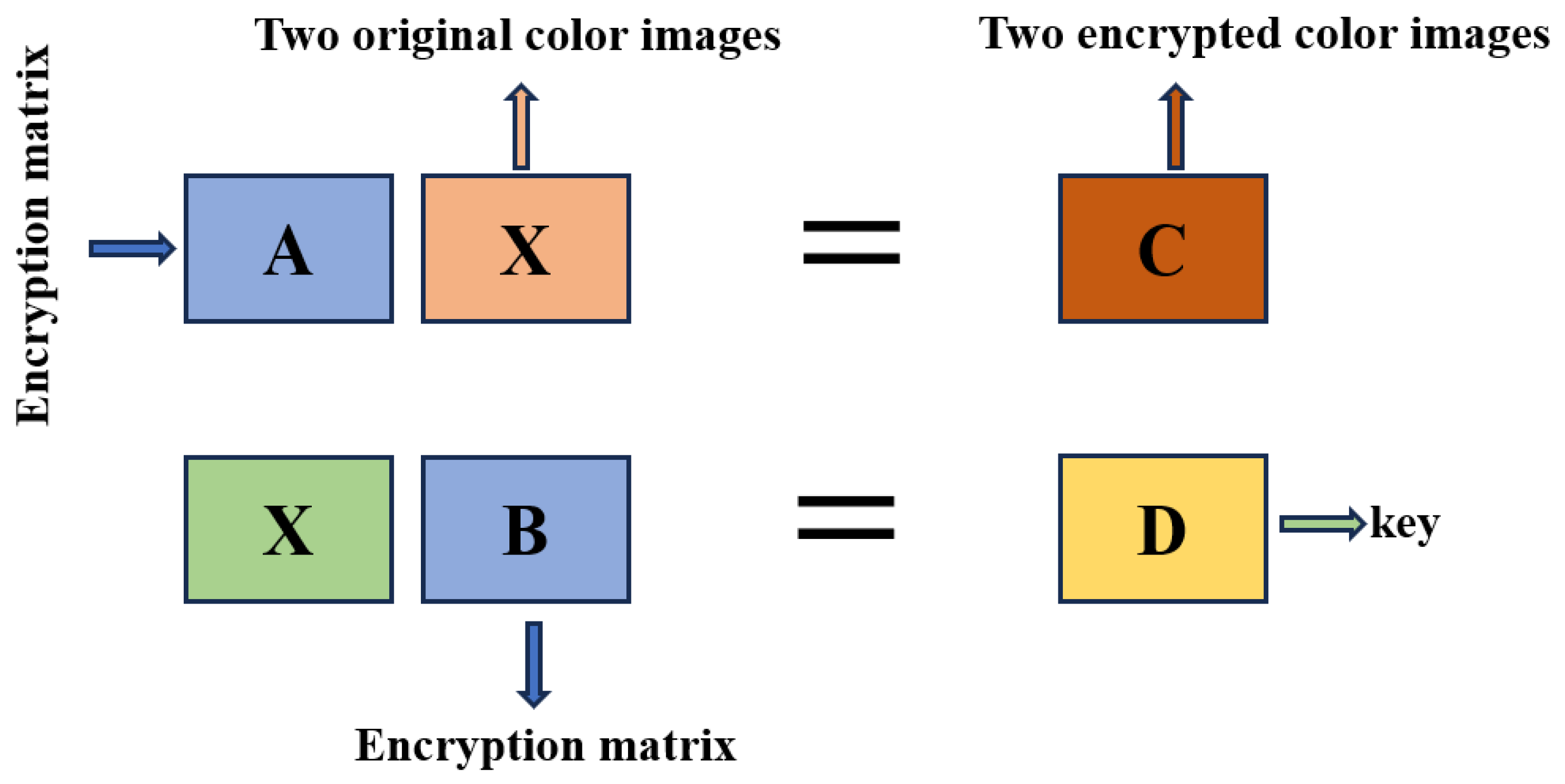
Figure 2.
The original, encrypted, and decrypted color images.
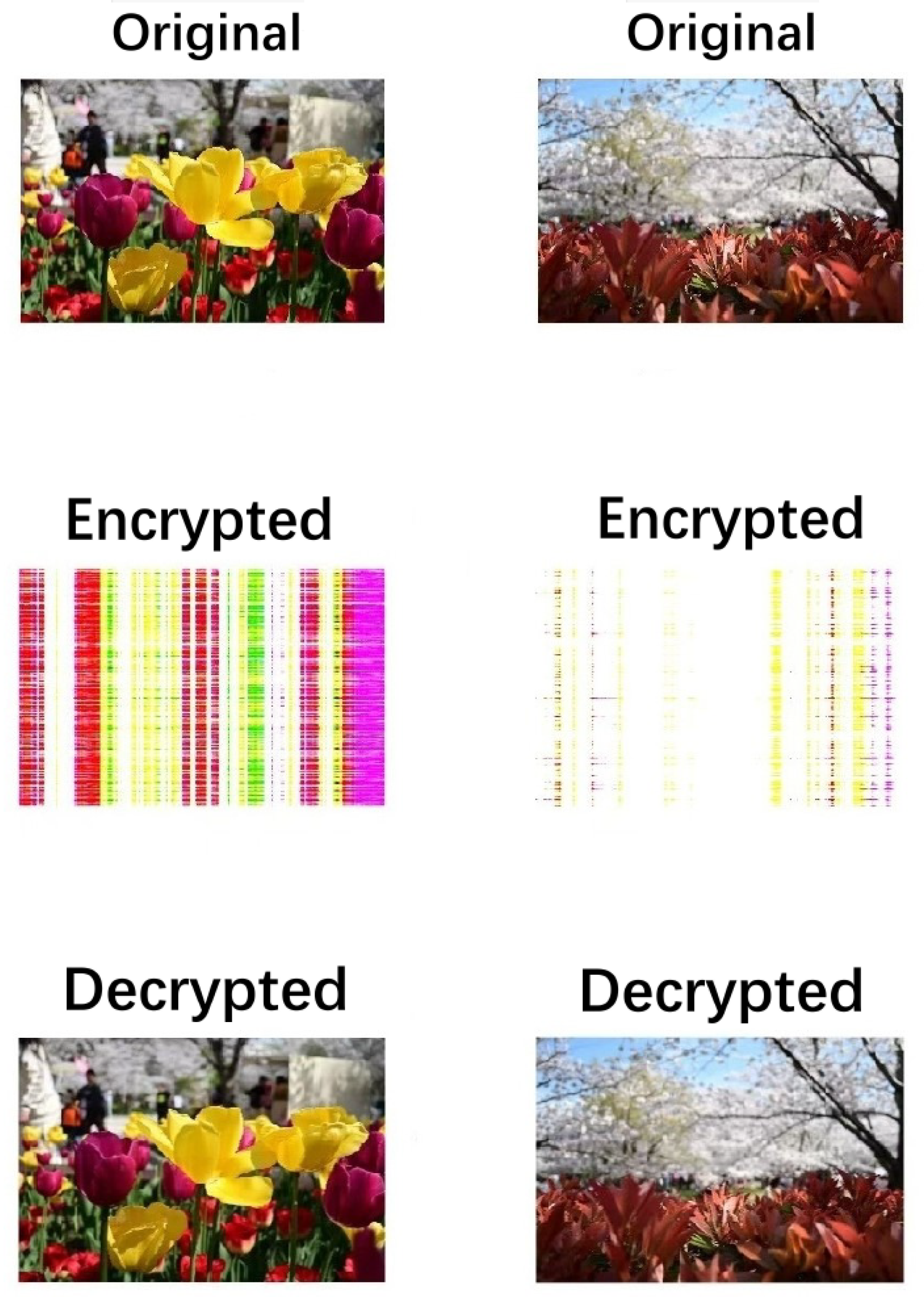
Figure 3.
The original, encrypted, and decrypted images of randomly selected slices from color videos.
Figure 3.
The original, encrypted, and decrypted images of randomly selected slices from color videos.
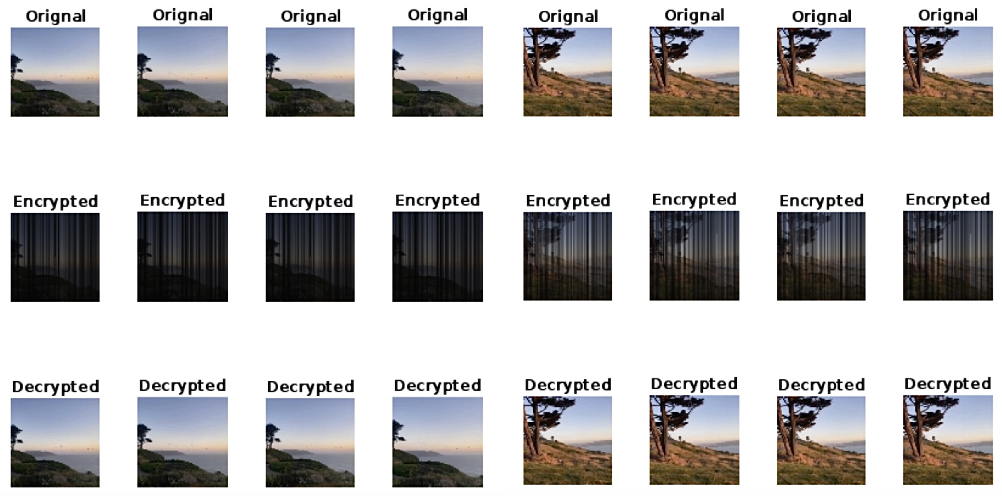

Table 1.
Definition of (anti-) Hermitian generalized (anti-)Hamiltonian matrices
| Symbols | Types of matrix | |
|---|---|---|
| non-trivial anti-symmetric orthogonal matrix | ||
| Hermitian generalized Hamiltonian | and | |
| Hermitian generalized anti-Hamiltonian | and | |
| anti-Hermitian generalized Hamiltonian | and | |
| anti-Hermitian generalized anti-Hamiltonian | and |
Disclaimer/Publisher’s Note: The statements, opinions and data contained in all publications are solely those of the individual author(s) and contributor(s) and not of MDPI and/or the editor(s). MDPI and/or the editor(s) disclaim responsibility for any injury to people or property resulting from any ideas, methods, instructions or products referred to in the content. |
© 2025 by the authors. Licensee MDPI, Basel, Switzerland. This article is an open access article distributed under the terms and conditions of the Creative Commons Attribution (CC BY) license (http://creativecommons.org/licenses/by/4.0/).
Copyright: This open access article is published under a Creative Commons CC BY 4.0 license, which permit the free download, distribution, and reuse, provided that the author and preprint are cited in any reuse.


