
Submitted:
03 April 2025
Posted:
03 April 2025
You are already at the latest version
Abstract
Large amounts of high-quality data is required for the training of Artificial Intelligence (AI) models, which are indeed cumbersome to curate and perform quality assurance via human intervention. Moreover, models trained using erroneous data (human errors, data faults) can cause significant problems in real-world applications. This paper proposes an automated cleaning framework and quality assurance strategy for 2D object detection datasets. The proposed cleaning method was designed according to the ISO/IEC 25012 data quality standards, and uses multiple AI models to filter anomalies and missing data. In addition, it balances out the statistical unevenness in the dataset, such as the class distribution and object size distribution. Thereby ensuring the quality of the training dataset and examining the relationship between the amount of data required for enhanced performance in terms of detection. The experiments were conducted using popular datasets for autonomous driving, including KITTI, Waymo, nuScenes and publicly available datasets from South Korea. An automated data cleaning framework was employed to remove anomalous and redundant data, resulting in a reliable dataset for training. The automated data pruning and assurance system demonstrated the ability to substantially decrease the time and resources needed for manual data inspection.
Keywords:
dataset pruning
; dataset whitening
; quality assurance
; noisy labels
; training data
1. Introduction
Artificial intelligence (AI) technology has rapidly developed, achieving remarkable results in fields such as autonomous driving [1,2], and healthcare [3]. These advances require four key elements: the model, data, hardware, and software. High-performance hardware leverages data and software to create AI models and efficiently train them. To improve AI models further, experts have emphasized the importance of large amounts of high-quality data [4,5,6]. These processed data play a crucial role in effectively training the AI models. The amount of high-quality data required for training AI models is a significant factor in yielding reliable AI models. These data, which serve as inputs for the model training, should be free of anomalies. Data labeling is typically performed to generate large datasets and so, human operators with basic knowledge and experience in data processing are required. However, manual labeling has limitations in terms of the number of available operators and unforeseen human errors. Additionally, differences in workers’ backgrounds and expertise can lead to biases and anomalies.
Developing a systematic method to enhance data quality is essential. The ISO/IEC 25012 [7] standard, as well as the “Data Quality Management Guidelines for AI Training" [8] published by the Korean Ministry of Science and the National Information Society Agency, provide procedures and principles for managing and evaluating data quality. The "Data Quality Model" measures the level of data quality and is categorized into six main categories: accuracy, completeness, consistency, reliability, validity, and expressiveness. A study [9] highlighted the importance of quality verification in ensuring the reliability and validity of data by focusing on quality assurance using standards. Another study [10] utilized an ontology-based method to evaluate data quality according to standards, and established metrics for functionality and reliability. A previous study [11] demonstrated the use of metrics derived from standards to assess and enhance the quality of data.
Model-centric methods that optimize model structure and function have been used to improve the performance and reliability of AI models [12,13]. Some studies have proposed new loss functions to minimize the effect of noisy labels and train noise-robust models [14,15,16,17]. However, changing the model structure could solve certain problems. Therefore, data-centric methods are essential [18,19] for efficient data collection, classification, pruning, and processing to construct training datasets [20,21,22]. There are studies on Noisy Label Learning (NLL) [23,24,25] that aim to improve the generalization performance of models using training data with noisy labels, rather than overcoming noisy data. These studies have proposed introducing new types of noise or methods to distinguish challenging data. Flawed data can degrade the performance of AI model training or cause erroneous results [26,27,28]. A previous study [29] outlined the training of deep-learning models with noisy labels and presented a method for correcting label noise. Similarly, data preprocessing, such as removing or correcting data with anomalies, is required [30,31].
Previous studies investigated the importance of datasets in training models [32]. The authors proposed a cross-validation framework using various convolutional neural networks (CNNs) to validate data quality and efficiency. Focusing on label correlation, another study [33] proposed a method to enhance multi-label annotation using noisy crowdsourced data. A framework [34] for identifying and correcting noisy labels in crowdsourced labeled datasets also exists. Several correction algorithms [35,36] have been proposed to address noise interference when datasets containing noisy labels are used. These algorithms use a consensus voting method to solve the noisy label problem. A label enhancement method [37] was developed to refine label distributions and improve the classification performance in noisy datasets by utilizing trusted data. Several studies [38,39,40,41,42] have adopted active learning as a model-training strategy to iteratively improve the model performance by reconstructing data. Effective relabeling through prioritization can improve dataset quality.
In a practical training dataset, it is essential to ensure that each label is unbiased and that there is no duplicate data. If models are trained on biased datasets, they may not perform well on other test sets. Therefore, methods such as data preprocessing or exclusion should be employed during training [43,44,45]. One study [46] computed the density from the class distribution of objects in redundant data by selecting the best data sample for model training. Some studies [47,48,49] investigated the correlation between data quality and AI model performance using data quality assessments. One study [48] used a machine learning model to check label quality in an object detection project. A small high-quality dataset was reprocessed from one that required quality validation and trained using a neural network for quality validation. One study [50] focused on selecting optimal instances from datasets with imperfect labels, and proposed algorithms that prioritize data subsets based on their expected labeling quality.
2. Methodology
In this study, we propose an automated process to ensure the quality of autonomous driving (AD) datasets for 2D object detection AI models by removing outlier data and normalizing the distribution. As shown in Figure 1, a framework is introduced that prevents contamination by anomalous data and enables effective learning by eliminating redundancies and bias. The first step involves discarding noisy labels. A labeling score was introduced that employs inference results from multiple AI models to evaluate data anomalies. Subsequently, the data distribution is whitened. The diversity scores were calculated by comprehending the class and bounding box size distributions. Based on these scores, the system prioritizes the data and proceeds with data reduction.
In this study, a dataset pruning process was used to remove abnormal data from the dataset, and whitening the distribution. Thus, automated quality assurance was executed through the utilization of an AI model rather than manual examination, thereby achieving the following technical benefits.
- Automated quality assurance of the AI training dataset.
- Calculation of data quality indicators through prediction results of the trained model.
- Calculation of statistical indicators to satisfy statistical diversity and eliminate bias.
- Reducing the amount of data required for training.
- Automatic classification of data requiring re-annotating.
The remainder of this paper is organized as follows. Section 3 describes the deletion of noisy labels and automatic detection and removal of abnormal data. Section 4 describes the process of whitening the data distribution, wherein the data are reduced based on the distribution. Section 5 provides both qualitative and quantitative outcomes, showing the enhancement in the performance of the model resulting from the eradication of noisy labels and distribution whitening. Section 6 analyses the overall experimental outcomes of the study and their influence on the subsequent research practices in the field and Section 7 concludes the research study.
3. Proposed System: Deleting Noisy Labels
3.1. Overview
The first step in this study was to pinpoint and remove noisy data, such as that depicted in Figure 2. This involved presenting examples of both clean and noisy labels by using the six datasets employed in the investigation. The first column represents the ideal case with clean labels. The second column shows examples in which objects were assigned incorrect classifications or misaligned bounding boxes. The third column shows examples in which the bounding box does not completely enclose the object. The fourth column indicates cases in which a label is absent for an object that requires it. The last column presents examples of Ground Truth (GT) damage during processing and storage.
To guarantee the quality of the AI datasets, several institutions perform visual inspections to verify the data for errors or inaccuracies. However, this procedure requires human intervention, and examining the entire dataset is challenging, time consuming, and costly. Our research project trained an AI model and employed it to identify and rectify anomalous data in an entire dataset. As depicted in Figure 3, the process of deleting noisy labels proceeds in three stages: model training, labeling score ensemble, and deletion. The deletion phase computes the deletion achievement to determine whether to repeat or terminate the noisy label deletion process.
3.2. Defining LScore
In this study, a “Labeling Score (LScore)” was defined to automatically detect noisy data. The ISO/IEC 25012 standard outlines characteristics for assessing data quality independently of specific systems or environments. LScore is based on the indicators of accuracy, completeness, and credibility, which are used as data quality verification indicators. Accuracy measures how well data represent actual values and uses the intersection over union (IoU) metric to calculate the overlap between model-influenced and GT bounding boxes for each object in the frame. Completeness verifies the inclusion of all expected instances and is ensured through recall, an activation function that ensures all valid objects in a frame are labelled. Credibility evaluates data trustworthiness from the user’s perspective and is verified via the confidence score, which represents the precision of a model’s inference for each entity in a frame. Each object in the generated dataset is evaluated to determine whether the label is correct for the class.
3.3. Model Training
There is a process for the inspector to complete the correct answer sheet to ensure GT. In this study, the prediction results of the 2D object detection model were used. Detectron2 [51], a PyTorch-based object detection library, was used for efficient training. Submodels a, b, and c based on Faster R-CNN [52] with similar performances (R101-C4, R101-DC5, and R101-FPN) were trained. An evaluation model, RPN R101-FPN, was trained based on RPN and Fast R-CNN [53]. Hyperparameters were slightly adjusted from the default values provided by the Detectron2 library to fit the experimental environment, with a learning rate of , a batch size of 8, and 5000 iterations. The trained submodels a, b, and c were used for ensemble LScores. The evaluation model was used to evaluate the performance of the remaining dataset after deleting the erroneous data. From each dataset, 20% of the data was fixed as the validation set, and the remaining 80% was split into three equal subsets for training. Submodels a, b, and c used a randomly split subset of the dataset with a 33:33:34 ratio. Repeated noisy label deletion computes the LScore threshold for the initial validation dataset. The dataset did not change, but the model was iteratively trained to gradually remove noise and improve performance. Therefore, we used the score threshold of the initial validation dataset to remove the noisy labels.
3.4. LScore Ensemble
In this step, LScores are ensembled to automatically detect noisy labels and proceed with their deletion. The submodels trained on separate subsets of data, namely a, b, and c, were verified on their respective validation datasets to determine the threshold for the LScores. Using the computed LScores and thresholds, a decision was made to retain and remove the data.
3.4.1. Calculation of the E’LScore Threshold
The E’LScore (Ensembled Labeling Score) Threshold is a criterion used for the automatic detection of noisy data. If the LScore calculated for the training dataset did not exceed the threshold, the data were considered noisy and were removed. The threshold itself is based on the averaged LScore, making it a value optimized to the dataset. By using a dataset-defined threshold, comparisons are made against values internal to the dataset, ensuring that the threshold is specifically aligned with the dataset’s characteristics.
LScore: It is a numerical measure of the quality of each frame. This is defined as a mathematical value that combines accuracy, precision, and recall. Accuracy is based on the IoU between the GT and the inferred bounding box. Precision is determined by the confidence score for the classified bounding box class, and recall is calculated based on the true-positive results. To represent the dataset inferred by the trained model, is defined as the submodel, and represents the parameters used in training submodel . The inference results for the validation dataset of subset are expressed as . The labeling score , is calculated using equation (1):
where the weight of each bounding box satisfies the condition defined in equation (2):
and is the number of bounding boxes predicted by the submodel, with weights calculated according to equation (3):
is the total number of data constituting the subset and is the average LScore calculated for the data . The average value is obtained by dividing the sum of by the number of bounding boxes that satisfy the condition. The number of bounding boxes that satisfy this condition is denoted by .
E’LScore Threshold: This is the process of obtaining the LScores for all frames of the validation dataset of each subset and ensembling the , the average LScore. is obtained using equation (4):
where represents the number of submodels. This was the average of the mean LScores of the other submodels, excluding one submodel.
3.4.2. Calculation of the E’LScore
By combining the inference results of the models, the E’LScore was used as a criterion for voting among the cross-validation methods. For a certain dataset, the average value was derived by calculating the LScore for each data by inference using a model trained with another subset.
E’LScore: The E’LScore follows the same approach as that described in Section 3.4.1. For a different submodel, the LScore for each frame in the training dataset is denoted by which corresponds to the number of bounding boxes predicted by the submodel for the frame. Each bounding box in is associated with its weight that satisfies the condition in (2) . The E’LScore combines the LScores obtained from the different submodels for the same training dataset. Thus, for the datum from to , the average LScore calculated for each frame is combined and averaged as described in (5):
The combined E’LScore was used as the final comparison score for noisy label deleion.
3.5. Deleting Ratio Score
The dataset was refined by automatically detecting and deleting abnormal data by comparing the ensemble label score with the E’LScore threshold. The data to be deleted are labeling errors or missing labeling data, and data that do not help in training by acting as noise in the learning process. According to condition P specified in (6):
the remaining data and the data to be deleted were determined for the training dataset of each subset. The dataset was then refined and organized based on (7):
During each iteration of the noisy label deletion process, the deletion achievement was calculated to achieve the recommended criterion for a semantic accuracy of 95%, according to [8]. Specifically, suppose that the proportion of data marked for deletion is 95% or higher relative to the original data quantity before the noisy label deletion process. In this case, the noisy label deletion process is halted. Finally, the remaining data, excluding the deleted data, were utilized in the data distribution-whitening step. The deletion process was quantified using the deletion ratio, as shown in (8):
that calculates the ratio of the data count after deletion to that before deletion.
4. Proposed System: Whitening Data Distribution
4.1. Overview
The whitening data distribution balances the distribution of the classes and sizes of the objects in a dataset. It is important to consider the quantity and proportion of value objects for training. The whitening score quantifies the semantic concepts of standards and guidelines to identify statistical variability and reconstruct unbiased data. The whitening data distribution process consisted of three main steps: diversity score calculation, data whitening, and model training. These steps are executed in the order shown in Figure 4. The diversity scores comprise the scores for the class and bounding box size distributions. The final whitening score was calculated by integrating the previously used as a bias value for noisy label deletion. The data were sorted by whitening score, and low-priority data were excluded from the training dataset when training the model.
4.2. Diversity Score
The diversity score indicates the rarity of the classes of objects that comprise each frame and the object sizes. Class distribution is the number of bounding boxes that belong to each class in the dataset. The bounding box size distribution describes the size distribution of the bounding boxes that comprise all frames in the dataset. The bounding box was divided into specific ranges from the minimum to the maximum size, and the number of bounding boxes in each range was counted. Diversity scores use z-scores, also known as standard scores, which use standard deviations and variances. A negative z-score for a small data distribution indicates a below-average occurrence, while a positive z-score for a wide distribution signifies an above-average occurrence. This polarity shows the frequency of each data point relative to the mean. Reversing the z-score sign assigns higher values to rare objects, emphasizing their uniqueness. This method highlights infrequent data points, enabling the model to better identify and prioritize rare objects during training.
4.2.1. Calculation of the CDScore
The “Class Diversity Score (CDScore)" indicates that the standard score obtained for each item in the class distribution was calculated and averaged over all the bounding boxes in the frame. The class distribution list was created by counting the classes of labeled objects constituting the frame for each frame of the entire dataset. In dataset , after deleting noisy labels, the number of objects belonging to class k in dataset is the total number of pairs, where is k. The distribution list , is expressed as (9):
and the class distribution list is composed of pairs of each class and number of objects belonging to class .
Utilizing the class distributions obtained in (9), we generated a list of mean values, variances, standard deviations, and deviations from the distribution. Algorithm 1 is a function that receives a distribution list, normalization, and the number of distribution items as input, and returns a normalized standard deviation and a deviation list, where each item’s deviation value is multiplied by . In the algorithm, norm_list ← [0] x cnt_factor is used to initialize a list called norm_list with a length of cnt_factor, where all elements are set to 0. These values are necessary for calculating the CDScores.
| Algorithm 1:Normalized Deviation List Generator. |
|
After normalizing the distribution list, the variance is obtained as shown in (10):
The distribution value for items is the number of items in each distribution type, and the average value is . The deviation is the difference between the distribution value and the average, and the value divided by the standard deviation is the z-score, as shown in (11)
In the CDScore calculation, class z-scores corresponding to the bounding boxes constituting the frame were added and averaged. To accomplish this, we used , which lists the z-scores of each item in the class distribution.
The CDScore (12) is calculated for each data point , where in dataset after noisy labels have been removed, using the following equation:
For all bounding boxes from to labeled as , the bounding box class is . The z-score of the bounding box takes a value corresponding to the corresponding class from . For all bounding boxes, the value obtained by adding all elements of corresponding to and averaging was calculated as the CDSCore of the corresponding data . All bounding boxes are treated equally in this calculation, with no weighting applied.
4.2.2. Calculating BSDScore
The “Bounding box Size Diversity Score (BSDScore)" is the average of the standard scores obtained for each item in the bounding box distribution. The bounding box size distribution measures the size of all the bounding boxes in a dataset. A standard score was derived by classifying the range from the minimum to maximum size into five intervals of 20% each. The bounding box size r is defined by dividing the minimum bounding box size by the maximum bounding box size into five intervals, as shown in (13):
In dataset , , that is, the number of objects belonging to the bounding box size r is the number of all pairs, where is r. The distribution list based on this definition is represented in (14):
Using the bounding box size distribution list obtained from (14), the standard deviation and deviation lists are derived using Algorithm 1. A z-score was calculated for each bounding box size interval to derive the list obtained using the following equation (15):
To obtain the BSDScore for one data point, the value is obtained by adding all elements of corresponding to and averaging the value of the corresponding data . The BSDScore, is calculated using (16), as follows:
4.3. Calculating Whitening Score
Data whitening was used to measure the statistical diversity of a dataset and to adjust for imbalances in the data. This process sorts the data to prioritize the data to be reduced. Data with a low priority were excluded from the dataset based on the reduction rate. The data were reduced by 10% from the initial 100%, and the difference in performance according to the whitening score was analyzed. The RPN R101-FPN model based on a Fast R-CNN was used as the evaluation model. This was used to determine the optimal degree of reduction by comparing the performance of the models after the reduction.
The CDScore was combined with the BSDScore. The E’LScore is used to detect noisy labels and represents the bias value. The whitening score for data , where , included in dataset from which the noisy labels were deleted, is calculated as shown in (17):
The final diversity score, obtained by multiplying each diversity score (CDScore and BSDScore) by and then adding them together. This weighting with represents the equal contribution of each score to the final diversity score. Priority was given to the data based on the whitening score for the final data whitening task. The Whitening Score in (18) is as follows:
and from (5) were added as the bias values.
The E’LScore (5) from Section 3 was used to calculate the whitening score. There were also data points with low diversity scores. These data are not sparse in terms of class or object size. However, training a model using immature data is beneficial. Only the GT was used for the diversity score calculation. The E’LSCore is necessary because it does not include judgments on whether it benefits learning. Figure 5 shows the necessity of combining E’LScores. Figure 5(a) shows the rare classes of buses and bicycles. Nevertheless, the bus belongs to the wrong class and the bike has an unclear bounding box. A human object has a high BSDScore score, but a low whitening score because it is a typical class. However, the objects depicted in Figure 5(b) are two vehicles and a person; both standard classes and bounding box sizes are also not rare. However, the whitening score was high because all object labeling and class matching were correct.
5. Experiments and Results
5.1. Experimental Setup
This study introduces a method to ensure the quality of a 2D object detection model training dataset through a verification process. This process entailed training four models per iteration to eliminate noisy labels. In addition, one model was trained during the data distribution whitening process. Experiments were conducted on a PC equipped with an Intel Core i9-7900X 3.3GHz CPU, 62GB RAM, and two NVIDIA GeForce 1080Ti GPUs. The Detectron2 library was used to train the 2D object detection model. Details regarding model training are provided in Section 3.3 and Section 4.3. These experiments revealed the issues present in the dataset and highlighted the importance of using a dataset with a guaranteed quality. Table 1 presents a comparison of the features of the datasets used in this experiment. The study utilized autonomous driving datasets such as the KITTI [20], Waymo [21], and nuScenes [22] datasets. Road Driving Image Data (RDID) [54] and Autonomous Driving Data in Various Weather Conditions (ADVWC) [55] were obtained from AIHub, whereas Generic and Edge Case Scenario Data (GECSD) were obtained from the Korea Transportation Safety Authority (KOTSA) [56].
5.2. Results of Deleting Noisy Labels
Noisy labels were detected and removed automatically from the dataset. The influence of data pruning on the model training and recognition performance was investigated using a fast RCNN-based R101-FPN model as an evaluation tool. Accuracy was assessed using the AP50 metric. AP50, which represents Average Precision at IoU = 0.5, evaluates the object detection performance. A detection is correct if the IoU between the predicted and actual bounding boxes is at least 0.5, with average precision calculated under this criterion. This metric signifies the model’s detection accuracy, and in this study, AP50 was used to rigorously assess model performance improvements. During the framework iterations, the training data were decreased by eliminating anomalous data. Table 2 presents the experimental results of deleting noisy labels from the six datasets, which are presented in Table 2. The number of process iterations, deletion achievements, and best iteration points for each dataset were compared to those of the previous process. Despite the reduction in the training data, the performance improved across all datasets owing to the classification of the noisy labels. For Waymo and RDID, the deletion amount was up to 2%,confirming that they were clean datasets with almost no noise labels. The data classified as noisy labels were either empty with no objects or too complex for the model to interpret.
Labeling errors, missing labeling data, and data that interfered with the training process are filtered and deleted as noisy labels. The labeling error data were removed when the LScore was below a certain threshold. This occurred when there was a significant difference between the results predicted by the model and GT. Label-inaccurate data were those with the correct label classification but inconsistent magnitudes when the prediction model and GT results were compared. In other words, the bounding box either partially encloses the object or is too large. Missing labeling data occur when there is no labeling in the GT, even though the model detects an object with a high confidence score. In other words, the data differs from the correct answer when the model predicts the input, even if it is judged as essential information.
Figure 6, Figure 7, Figure 8 and Figure 9 show examples of filtered noisy labels. For each image, the GT labeling data are displayed on the left, whereas the prediction result of one of the sub-models is shown on the right. Each image below shows an enlarged view of the area containing this error. A noisy label was identified by comparing the predictions made by the submodel with the GT. Therefore, the greater the difference between the two, the higher the likelihood of erroneous data. For the KITTI data, Figure 6(a) shows labeling errors for objects reflected on the exterior of the car. The submodel failed to predict cars reflected on the bus, resulting in a low E’LScore. Consequently, the data should be considered for deletion. Figure 6(b) filters out labels with incorrect bounding box areas for pedestrians. Because of the excessive size of the bounding box encompassing pedestrians, unnecessary pixel information may be used by the model. Figure 6(c) shows incorrect labels for pedestrian objects and missing labels for cyclist objects.
In the nuScenes dataset, errors were present when the truck bounding box was double-labeled on the car object, as shown in Figure 7(a). These errors are common when auto-labeling machines are employed. In addition, there are instances in which the label is missing for the car object, as shown in Figure 7(b). These errors can cause confusion when calculating the loss of a model. An inaccurate bounding box for a truck object, as shown in Figure 7(c), is another concern. In the GT, the bounding box size is larger than that of the submodel.
The ADVWC dataset contains bad weather data, such as heavy rain and fog, and many objects are unclear, as shown in Figure 8(a). If the submodel predicted a blurry bollard object while the GT did not, it was categorized as erroneous. Despite the adverse weather conditions, the model must consistently provide accurate predictions. Labeling for car objects with only headlights visible in heavily fogged data and for small and detailed objects is omitted, as shown in Figure 8(b). In Figure 8(c), an object labeled as a central reservation is mistakenly categorized as a bollard.
The GECSD dataset, which contains over pieces of data, is so extensive that numerous crowd workers are required for labeling. Unfortunately, owing to an error in the data storage process, there are instances in which the labels have been mistakenly altered, as illustrated in Figure 9(a) and Figure 9(b). In these instances, a traffic sign is incorrectly labeled as a bus or a car as a bicycle, which makes it challenging for the model to provide consistent predictions for the same object. Figure 9(c) depicts the data that has been filtered to remove the missing labeling. These data were collected during nighttime, and because the objects in the images were relatively small, crowd worker declined to provide annotations. Consequently, the trained model generated predictions for these objects, resulting in their exclusion as erroneous data during the LScore calculation process. The ADVWC and GECSD datasets exhibit a performance difference of up to before and after the process, with data that is not suitable for human judgment removed. Data distribution whitening experiments were performed using the data remaining after deletion.
5.3. Results of Whitening Data Distribution
The CDScores and BSDScores are calculated to determine the whitening score, which serves as the basis for priority. The whitening score was used to assess the suitability of the data for meaningful utilization in the model training. To reduce the amount of data, a specified priority was assigned based on the degree of data reduction, which ranged from 100% to 50%. The data reduction rate was varied in increments of 10%. The results for the six datasets are presented in Table 3. The best reduction rate, accuracy, and number of data points are compared. The accuracy values in parentheses indicate the increase compared to the accuracy before whitening, which is the improved AP50 value after noisy label deletion. In these experiments, data reduction was conducted based on priority, and its impact on model prediction performance was examined. The highest performance was achieved at 20% or 30% reduction for all datasets. The best reduction in the whitening process is referred to as the best reduction for each dataset. Accuracy, derived from the highest degree of reduction, was used to evaluate the performance of the model. The same validation dataset was used for all reduction processes. The detection performance increased by up to for the KITTI and nuScenes datasets. In other datasets, the performance improved even further despite the reduction in the data used for training.
The whitening process reduces data for non-rare classes or non-sparse bounding box sizes. The dataset used in the experiment was composed of autonomous driving data collected and processed on a road. Consequently, data from vehicles on the road has a lower priority. This is because object classes have the most extensive distribution, and the bounding box size for objects on the road is the most common. Figure 10(a) depicts the gradient of the class distribution values for the KITTI dataset. The hatched circles represent the class distributions before whitening, whereas the solid lines represent the class distributions after whitening. The class with the largest distribution, that is, cars, was reduced. The number of cars decreased from to and the number of trams decreased from 350 to 338. The distribution of rare objects such as trams, trucks, and vans remained relatively consistent. Figure 10(b) illustrates a bubble plot showing the changes in the bounding box size distribution values; the distribution for the sparse size did not change significantly.
Figure 11 shows an example of the data excluded from the distribution whitening process in the Waymo dataset. The number of cars decreased from to of pedestrians decreased by 202 and the number of bicycles decreased by 15. The priority is determined based on the distribution. Therefore, regular objects have lower priority than rare objects. Because of the presence of more clearly defined data than the given frame, the latter was excluded in the subsequent learning phase. However, the whitening data distribution process used in this study was uniform. Therefore, for datasets developed for specific purposes such as autonomous driving, it is necessary to adapt distribution techniques according to the laws of the natural environment.
The provided figure, denoted as Figure 12, illustrates low-priority data from the nuScenes dataset. Figure 13(a) and Figure 13(b) depict the class and bounding box size distribution gradients for the nuScenes dataset. Within the dataset comprising objects, items were assigned a low-priority status during the whitening process owing to redundancy or a lack of relevance to model training. In the class distribution, pedestrians had the highest number of objects followed by cars, barriers, and traffic cones. Specifically, in the pedestrian category, there was a reduction from to instances. The second notable decrease occurred in the car category with a reduction of 804 objects. Despite the reduction in object count, there was a notable improvement in the overall performance. After deleting noisy labels, AP initially stood at . However, after whitening, there was a significant performance gain, increasing by points, yielding an AP score of . This highlights the effectiveness of the whitening process in enhancing the suitability of the dataset for the learning tasks.
6. Discussion and Future Scope
This study proposes a dataset pruning framework and quality assurance that eliminate errors in autonomous driving datasets. It has the following characteristics.
- It automatically finds incorrect, inaccurate, missed, and damaged labels generated during the human annotation process.
- The training efficiency is increased by lowering the priority of duplicate or complex data and excluding it from the training dataset.
- Quality assurance, previously performed by humans on a small number of random pieces of data, can be automated on the entire dataset, saving time and money.
- It is easy to select data that need to be modified and reorganized into a high-quality dataset.
This study proved that not only a large amount of data but also high-quality data are vital for model learning. Data quality was automatically guaranteed by filtering the abnormal data and mitigating the imbalanced data. The model was trained using the dataset built during the noisy label deletion process, and the noisy label was distinguished using the prediction result. The data used for the training were obtained by gathering opinions from multiple models. In a previous study, several models were used [32]. However, the methods used to deterinme the data that should not be used differ. A trustworthy dataset [32] used single scores, such as F1 and accuracy. However, the proposed study quantified and utilized indicators defined in the standard. It is important to note that incorrect data may still be used during the initial submodel training, which makes the LScores calculated from the prediction results only partially reliable. The LScore calculation includes the confidence score and IoU value. If the overlap between the GT data and prediction bounding box is small, the LScore becomes negligible. This approach is particularly sensitive to small objects, ensuring that they are properly accounted for during the training. This issue can be addressed by adding a process that uses a high-quality dataset, initially selected by an inspector like [57]. Additionally, a data and performance verification process needs to be added after the model training steps in the deleting and whitening phases. This will allow for monitoring changes in model performance and verifying data quality. Repeatedly training the model to delete noisy label or whiten the data distribution can lead to overfitting. To address this, it is necessary to add modules that regularize the input data during training or implement early-stopping mechanisms by monitoring performance metrics.
This study will be expanded by testing various detection models to analyze how model diversity affects noisy label identification. The assessment of different detection models aims to aid in selecting the best model for removing noisy labels, thereby improving the robustness and generalizability of the method. In addition, a comparison with recent NLL techniques that use model-based strategies is planned. This comparison is expected to offer deeper insights into the effects of noisy labels on the model performance and highlight the benefits of a data-centric approach.
The diversity scores were calculated using a uniform distribution as the ideal value for data distribution whitening. A previous study [46] improved the quality of the dataset by defining its class density and analyzing its correlation with the accuracy of each class. Compared to our study, Sutdy [46] is similar in that it confirms the diversity of the classes. Similarities with the learning data were also measured. Through dynamic data reduction using a binary search technique, only the data necessary for learning were retained and the performance change was confirmed. However, our study confirmed the class and object size distributions. There was also a significant difference in the calculated z-scores for the standard deviation. Through this study, the z-score could identify rare objects that were continuously included in the learning process. Conversely, duplicates or too many subjects were excluded from the study. However, 2D object detection data, particularly autonomous driving data, have been developed for specific purposes. Because we collected data from roads, vehicle objects accounted for more than half of all the objects. However, because the distribution of the actual environment was not considered in the diversity score calculation, it was necessary to follow a natural distribution.
This study aimed to automatically perform quality assurance by performing pruning on a dataset constructed by deleting noisy labels and whitening the data distribution. Cross validation of multiple models was performed to clean the dataset and ensure reliability of the purification criteria. Abnormal data that interfered with learning were automatically classified. The datasets were refined to reduce the data count and hardware overhead. However, the recognition performance of the trained model either improved or remained unchanged. Recently, there have been studies focused on mitigating the impact of noisy labels [58]. A comparative study is needed to determine which is more effective: reducing noisy labels through model-centric approaches or using noise-free datasets via data-centric methods like this study.
7. Conclusion
The study proposes a fully automated framework for validating publicly available datasets before use, using an AI model for the deletion of noisy labels and data distribution whitening. The framework is tested using six datasets published in South Korea and other countries. Data that is erroneous or harmful to the learning process is automatically filtered and excluded. The rare classes and objects necessary for data learning remain through the data-distribution whitening process. Duplicate data is then filtered. The combination of deleting noisy labels and whitening the data distribution is known as data pruning. Redundant or obstructive data is excluded, while only effective data is retained. This process reduces the total amount of data required for learning without significantly changing performance. The study adheres to the ISO/ICE 25012 data quality model standard and the ’Data Quality Management Guidelines for AI Learning’ of the Korea Ministry of Science and ICT and the Korea Intelligence Information Society Promotion Agency. The model’s accuracy, precision, consistency, and diversity are used as quality evaluation indicators. The proposed framework is versatile and can be applied not only to 2D object detection datasets but also to 3D object detection data and image semantic segmentation datasets.
Author Contributions
For research articles with several authors, a short paragraph specifying their individual contributions must be provided. The following statements should be used “Conceptualization, K.K. and H.K.; methodology, K.K.; software, K.K.; validation, V.K., K.K. and H.K.; formal analysis, K.K.; investigation, K.K.; resources, V.K. and H.K; data curation, K.K. and V.K; writing—original draft preparation, K.K.; writing—review and editing, V.K.; visualization, K.K.; supervision, H.K.; project administration, K.K.; funding acquisition, H.K. All authors have read and agreed to the published version of the manuscript.
Funding
This research was supported by the BK21 Four Program, funded by the Ministry of Education(MOE, Korea) and the National Research Foundation of Korea(NRF).
Data Availability Statement
The data underlying the conclusions of this article will be made available by the corresponding author upon reasonable request.
Acknowledgments
This research was supported by the BK21 Four Program, funded by the Ministry of Education(MOE, Korea) and the National Research Foundation of Korea(NRF). This research used datasets from ‘The Open AI Dataset Project (AI-Hub, South Korea)’. All data information can be accessed through ‘AI-Hub(www.aihub.or.kr)’.
Conflicts of Interest
The authors declare no conflicts of interest. The funders had no role in the design of the study; in the collection, analyses, or interpretation of data; in the writing of the manuscript; or in the decision to publish the results.
Abbreviations
The following abbreviations are used in this manuscript:
| AI | Artificial Intelligence |
| AP | Average Precision |
| ADVWC | Autonomous Driving Data in Various Weather Conditions |
| BSDScore | Bounding Box Size Diversity Score |
| CDScore | Class Diversity Score |
| CNN | Convolutional Neural Network |
| E’LScore | Ensembled Labeling Score |
| FPN | Feature Pyramid Network |
| GT | Ground Truth |
| GECSD | Generic and Edge Case Scenario Data |
| IoU | Intersection over Union |
| LScore | Labeling Score |
| RPN | Region Proposal Network |
| RDID | Road Driving Image Data |
References
- Ma, Y.; Wang, Z.; Yang, H.; Yang, L. AI applications in the dev. of autonomous vehicles: A survey. IEEE/CAA J. Autom. Sinica 2020, 7, 315–329. [Google Scholar] [CrossRef]
- Cunneen, M.; Mullins, M.; Murphy, F. Autonomous vehicles and embedded AI: The challenges of framing machine driving decisions. Appl. Artif. Intell. 2019, 33, 706–731. [Google Scholar] [CrossRef]
- Howard, J. AI: Implications for the future of work. Am. J. Ind. Med. 2019, 62, 917–926. [Google Scholar] [CrossRef]
- Roh, Y.; Heo, G.; Whang, S.E. A survey on data collection for ML: a big data-AI integration perspective. IEEE Trans. Knowl. Data Eng. 2019, 33, 1328–1347. [Google Scholar] [CrossRef]
- Mahmood, R.; Lucas, J.; Acuna, D.; Li, D.; Philion, J.; Alvarez, J.M.; Yu, Z.; Fidler, S.; Law, M.T. How much more data do i need? In estimating requirements for downstream tasks. In Proceedings of the Proc. IEEE/CVF Conf. Comput. Vis. Pattern Recognit. (CVPR); 2022; pp. 275–284. [Google Scholar]
- Whang, S.E.; Roh, Y.; Song, H.; Lee, J.G. Data collection and quality challenges in deep learning: A data-centric AI perspective. VLDB J. 2023, 32, 791–813. [Google Scholar] [CrossRef]
- Systems and Software Engineering - Systems and Software Quality Requirements and Evaluation (SQuaRE) - Data Quality with guidance for use. Standard, Int. Org. for Standardization, Geneva, CH, 2008.
- Ministry of Science and ICT of Korea, NIA of Korea. Data Quality Management Guidelines and Construction Guidelines for AI Learning 3 - Quality Management Guideline. https://aihub.or.kr/aihubnews/qlityguidance/view.do?pageIndex=1&nttSn=10125&currMenu=135&topMenu=103&searchCondition=&searchKeyword=, 2023.
- Gualo, F.; Rodríguez, M.; Verdugo, J.; Caballero, I.; Piattini, M. Data quality certification using ISO/IEC 25012: Industrial experiences. J. Syst. Softw. 2021, 176, 110938. [Google Scholar] [CrossRef]
- Lytvyn, V.; Vysotska, V.; Demchuk, A.; Bublyk, M.; Demkiv, L.; Shpak, Y. Method of ontology quality assessment for knowledge base in intellectual systems based on ISO/IEC 25012. In Proceedings of the IEEE 15th Int. Conf. Comput. Sci. Inf. Technol. (CSIT). IEEE, Vol. 1; 2020; pp. 109–113. [Google Scholar]
- Guerra-García, C.; Nikiforova, A.; Jiménez, S.; Perez-Gonzalez, H.G.; Ramírez-Torres, M.; Ontañon-García, L. ISO/IEC 25012-based methodology for managing data quality requirements in the development of information systems: Towards Data Quality by Design. Data Knowl. Eng. 2023, 145, 102152. [Google Scholar] [CrossRef]
- Liu, L.; Ouyang, W.; Wang, X.; Fieguth, P.; Chen, J.; Liu, X.; Pietikäinen, M. Deep learning for generic object detection: A survey. Int. J. Comput. Vis. 2020, 128, 261–318. [Google Scholar] [CrossRef]
- Zaidi, S.S.A.; Ansari, M.S.; Aslam, A.; Kanwal, N.; Asghar, M.; Lee, B. A survey of modern deep learning based object detection models. Digit. Signal Process. 2022, 126, 103514. [Google Scholar] [CrossRef]
- Li, J.; Socher, R.; Hoi, S.C. DivideMix: Learning with noisy labels as semi-supervised learning. arXiv:2002.07394, arXiv:2002.07394 2020.
- Mnih, V.; Hinton, G.E. Learning to label aerial images from noisy data. In Proceedings of the Proc. 29th Int. Conf. Mach. Learn. (ICML-12); 2012; pp. 567–574. [Google Scholar]
- Kim, Y.; Kim, J.M.; Akata, Z.; Lee, J. Large loss matters in weakly supervised multi-label classification. In Proceedings of the Proc. IEEE/CVF Conf. Comput. Vis. Pattern Recognit. (CVPR); 2022; pp. 14156–14165. [Google Scholar]
- Ghosh, A.; Manwani, N.; Sastry, P. On the robustness of decision tree learning under label noise. In Proceedings of the Proc. Pacific-Asia Conf. Knowl. Discov. Data Mining (PAKDD); 2017; pp. 685–697. [Google Scholar]
- Zha, D.; Bhat, Z.P.; Lai, K.H.; Yang, F.; Jiang, Z.; Zhong, S.; Hu, X. Data-centric Artificial Intelligence: A Survey. arXiv:2303.10158, arXiv:2303.10158 2023.
- Zhou, X.; Chai, C.; Li, G.; Sun, J. Database meets AI: A survey. IEEE Trans. Knowl. Data Eng. 2020, 34, 1096–1116. [Google Scholar] [CrossRef]
- Geiger, A.; Lenz, P.; Stiller, C.; Urtasun, R. Vision meets robotics: The KITTI dataset. Int. J. Robot. Res. 2013, 32, 1231–1237. [Google Scholar] [CrossRef]
- Sun, P.; Kretzschmar, H.; Dotiwalla, X.; Chouard, A.; Patnaik, V.; Tsui, P.; Guo, J.; Zhou, Y.; Chai, Y.; Caine, B. Scalability in perception for autonomous driving: Waymo open dataset. In Proceedings of the Proc. IEEE/CVF Conf. Comput. Vis. Pattern Recognit. (CVPR); 2020; pp. 2446–2454. [Google Scholar]
- Caesar, H.; Bankiti, V.; Lang, A.H.; Vora, S.; Liong, V.E.; Xu, Q.; Krishnan, A.; Pan, Y.; Baldan, G.; Beijbom, O. nuScenes: A multimodal dataset for autonomous driving. In Proceedings of the Proc. IEEE/CVF Conf. Comput. Vis. Pattern Recognit. (CVPR); 2020; pp. 11621–11631. [Google Scholar]
- Wang, W.; Li, Y.; Li, A.; Zhang, J.; Ma, W.; Liu, Y. An Empirical Study on Noisy Label Learning for Program Understanding. In Proceedings of the Proc. IEEE/ACM Int. Conf. Softw. Eng. (ICSE); 2024; pp. 1–12. [Google Scholar]
- Deng, L.; Yang, B.; Kang, Z.; Wu, J.; Li, S.; Xiang, Y. Separating hard clean samples from noisy samples with samples’ learning risk for DNN when learning with noisy labels. Complex Intell. Syst. 2024, 10, 4033–4054. [Google Scholar] [CrossRef]
- Zhang, J.; Song, B.; Wang, H.; Han, B.; Liu, T.; Liu, L.; Sugiyama, M. Badlabel: A robust perspective on evaluating and enhancing label-noise learning. IEEE Trans. Pattern Anal. Mach. Intell. 2024. [Google Scholar] [CrossRef] [PubMed]
- Natarajan, N.; Dhillon, I.S.; Ravikumar, P.K.; Tewari, A. Learning with noisy labels. Adv. Neural Inf. Process. Syst. 2013, 26. [Google Scholar]
- Song, H.; Kim, M.; Park, D.; Shin, Y.; Lee, J.G. Learning from noisy labels with DNNs: A survey. IEEE Trans. Neural Netw. Learn. Syst. 2022. [Google Scholar]
- He, H.; Garcia, E.A. Learning from imbalanced data. IEEE Trans. Knowl. Data Eng. 2009, 21, 1263–1284. [Google Scholar]
- Liu, D.; Tsang, I.W.; Yang, G. A convergence path to deep learning on noisy labels. IEEE Trans. Neural Netw. Learn. Syst. 2022. [Google Scholar] [CrossRef]
- Oleghe, O. A predictive noise correction methodology for manufacturing process datasets. J. Big Data 2020, 7, 1–27. [Google Scholar] [CrossRef]
- Xiong, H.; Pandey, G.; Steinbach, M.; Kumar, V. Enhancing data analysis with noise removal. IEEE Trans. Knowl. Data Eng. 2006, 18, 304–319. [Google Scholar] [CrossRef]
- Sun, Y.; Gu, Z. Using computer vision to recognize construction material: A Trustworthy Dataset Perspective. Resour. Conserv. Recycl. 2022, 183, 106362. [Google Scholar] [CrossRef]
- Zhang, J.; Wu, M.; Zhou, C.; Sheng, V.S. Active crowdsourcing for multilabel annotation. IEEE Trans. Neural Netw. Learn. Syst. 2022. [Google Scholar] [CrossRef] [PubMed]
- Zhang, J.; Sheng, V.S.; Li, T.; Wu, X. Improving crowdsourced label quality using noise correction. IEEE Trans. Neural Netw. Learn. Syst. 2017, 29, 1675–1688. [Google Scholar] [CrossRef] [PubMed]
- Zhang, C.; Zhang, H.; Xie, W.; Liu, N.; Li, Q.; Jiang, D.; Lin, P.; Wu, K.; Chen, L. Cleaning uncertain data with crowdsourcing-a general model with diverse accuracy rates. IEEE Trans. Knowl. Data Eng. 2020, 34, 3629–3642. [Google Scholar] [CrossRef]
- Wu, X.; Jiang, L.; Zhang, W.; Li, C. Three-way decision-based noise correction for crowdsourcing. Int. J. Approx. Reason. 2023, 160, 108973. [Google Scholar] [CrossRef]
- Xu, N.; Li, J.Y.; Liu, Y.P.; Geng, X. Trusted-data-guided label enhancement on noisy labels. IEEE Trans. Neural Netw. Learn. Syst. 2022. [Google Scholar] [CrossRef]
- Contardo, G.; Denoyer, L.; Artières, T. A meta-learning approach to one-step active learning. arXiv:1706.08334, arXiv:1706.08334 2017.
- Bernhardt, M.; Castro, D.C.; Tanno, R.; Schwaighofer, A.; Tezcan, K.C.; Monteiro, M.; Bannur, S.; Lungren, M.P.; Nori, A.; Glocker, B. Active label cleaning for improved dataset quality under resource constraints. Nat. Commun. 2022, 13, 1161. [Google Scholar] [CrossRef]
- Bachman, P.; Sordoni, A.; Trischler, A. Learning algorithms for active learning. In Proceedings of the Int. Conf. Mach. Learn. PMLR; 2017; pp. 301–310. [Google Scholar]
- Sener, O.; Savarese, S. Active learning for convolutional neural networks: A core-set approach. arXiv:1708.00489, arXiv:1708.00489 2017.
- Takezoe, R.; Liu, X.; Mao, S.; Chen, M.T.; Feng, Z.; Zhang, S.; Wang, X.; et al. Deep active learning for computer vision: Past and future. APSIPA Trans. Signal Inf. Process. 2023, 12. [Google Scholar] [CrossRef]
- Khosla, A.; Zhou, T.; Malisiewicz, T.; Efros, A.A.; Torralba, A. Undoing the damage of dataset bias. In Proceedings of the Proc. Eur. Conf. Comput. Vis. (ECCV). Springer; 2012; pp. 158–171. [Google Scholar]
- Li, Y.; Vasconcelos, N. REPAIR: Removing representation bias by dataset resampling. In Proceedings of the Proc. IEEE/CVF Conf. Comput. Vis. Pattern Recognit. (CVPR); 2019; pp. 9572–9581. [Google Scholar]
- Chen, H.; Chen, J.; Ding, J. Data evaluation and enhancement for quality improvement of ML. IEEE Trans. Reliab. 2021, 70, 831–847. [Google Scholar] [CrossRef]
- Byerly, A.; Kalganova, T. Class density and dataset quality in high-dimensional, unstructured data. arXiv:2202.03856, arXiv:2202.03856 2022.
- Chen, K.; Chen, H.; Conway, N.; Hellerstein, J.M.; Parikh, T.S. Usher: Improving data quality with dynamic forms. IEEE Trans. Knowl. Data Eng. 2011, 23, 1138–1153. [Google Scholar] [CrossRef]
- Pičuljan, N.; Car, Ž. Machine learning-based label quality assurance for object detection projects in requirements engineering. Appl. Sci. 2023, 13, 6234. [Google Scholar] [CrossRef]
- Li, C.; Mao, Z.; Jia, M. A real-valued label noise cleaning method based on ensemble iterative filtering with noise score. Int. J. Mach. Learn. Cybern.
- Fang, M.; Zhou, T.; Yin, J.; Wang, Y.; Tao, D. Data subset selection with imperfect multiple labels. IEEE Trans. Neural Netw. Learn. Syst. 2018, 30, 2212–2221. [Google Scholar] [CrossRef] [PubMed]
- Wu, Y.; Kirillov, A.; Massa, F.; Lo, W.Y.; Girshick, R. "Detectron2", 2019.
- Ren, S.; He, K.; Girshick, R.; Sun, J. Faster R-CNN: Towards real-time object detection with region proposal networks. Adv. Neural Inf. Process. Syst. 2015, 28. [Google Scholar] [CrossRef] [PubMed]
- Girshick, R. Fast R-CNN. In Proceedings of the Proc. IEEE Int. Conf. Comput. Vis. (ICCV); 2015; pp. 1440–1448. [Google Scholar]
- Korea Automobile ResearchInstitute. Road Driving Image Data. https://www.aihub.or.kr/aihubdata/data/view.do?currMenu=115&topMenu=100&aihubDataSe=data&dataSetSn=180, 2020.
- Korea National Information Society Agency. Autonomous Driving Data in Various Weather Conditions Dataset. https://www.aihub.or.kr/aihubdata/data/view.do?currMenu=115&topMenu=100&aihubDataSe=data&dataSetSn=630, 2021.
- Korea Transportation Safety Authority. Generic and Edge Case Scenario Data. https://avds.kotsa.or.kr/open/normal/Open_Normal_List.do?bbs_seq=3010, 2021.
- Chu, Z.; Zhang, R.; Yu, T.; Jain, R.; Morariu, V.; Gu, J.; Nenkova, A. Self-Cleaning: Improving a Named Entity Recognizer Trained on Noisy Data with a Few Clean Instances. In Proceedings of the Findings of the Assoc. Comput. Linguist. (NAACL2024); 2024; pp. 196–210. [Google Scholar]
- Chen, M.; Zhao, Y.; He, B.; Han, Z.; Huang, J.; Wu, B.; Yao, J. Learning With Noisy Labels Over Imbalanced Subpopulations. IEEE Trans. Neural Netw. Learn. Syst. [CrossRef]
Figure 1.
The overall framework of this study. We have noisy data or a dataset with an imbalanced distribution. Automated two-step process for refining the 2D object detection dataset. The noisy labels are filtered using multiple models, the diversity scores for class and bounding box size distribution are calculated, priorities determined, and assurance data without human intervention.
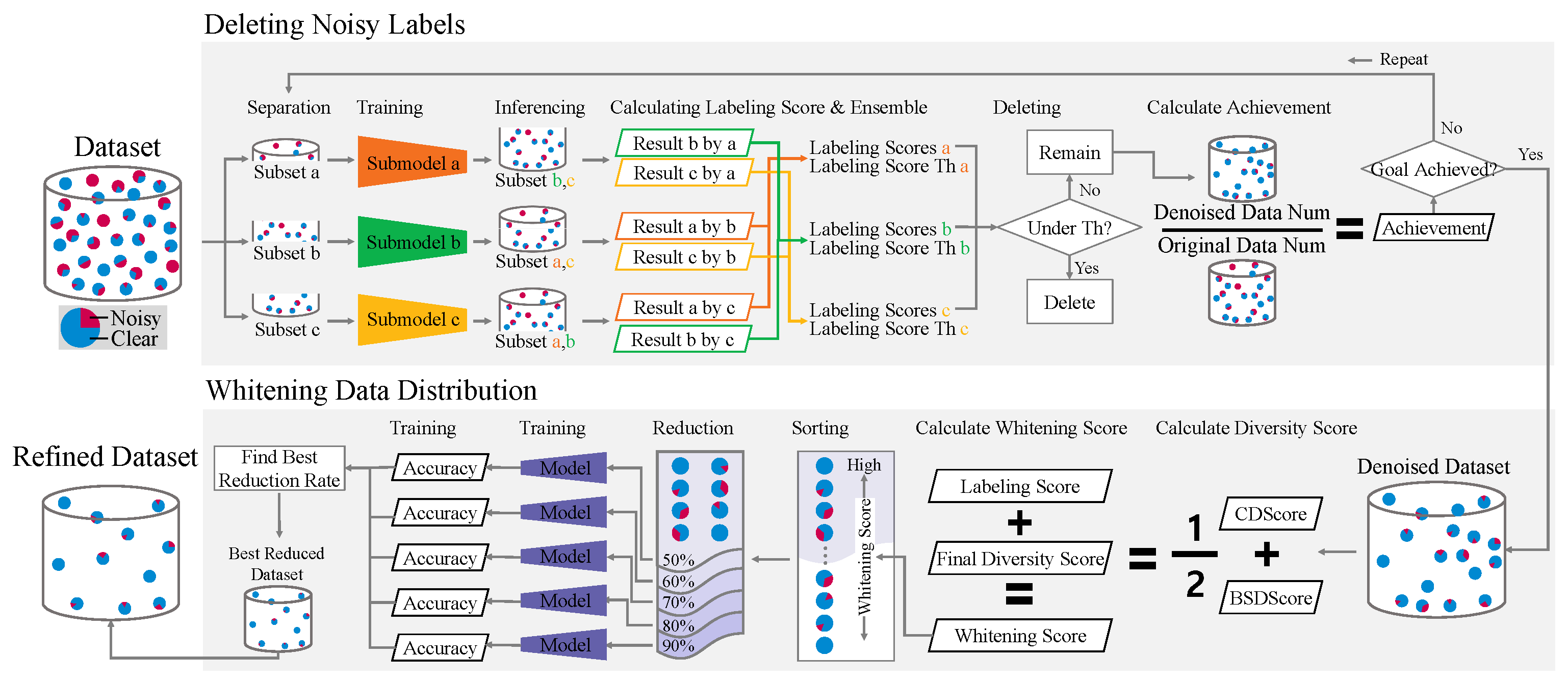
Figure 2.
Example of abnormal data. Col 1 is the data with clear labels. Col 2 is data with an error label, either the wrong class for the object or the wrong bounding box. Col 3 is inaccurately-labeled data with too large or too small bounding boxes. Col 4 is the data where the object is missing a label. The last column is corrupted data (error in label file, etc).
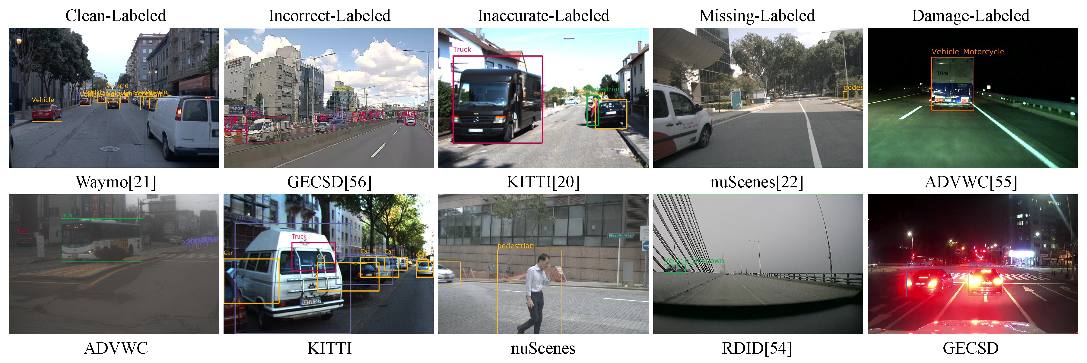
Figure 3.
Flowchart of the process of deleting noisy labels. This process operates in three steps: model training, labeling score ensemble, and deletion. Several models that automatically filtered noisy labels were trained. The ensembled labeling score determines the data to be deleted and the data to be retained. This process was repeated until 95% of the guidelines [8] were achieved.
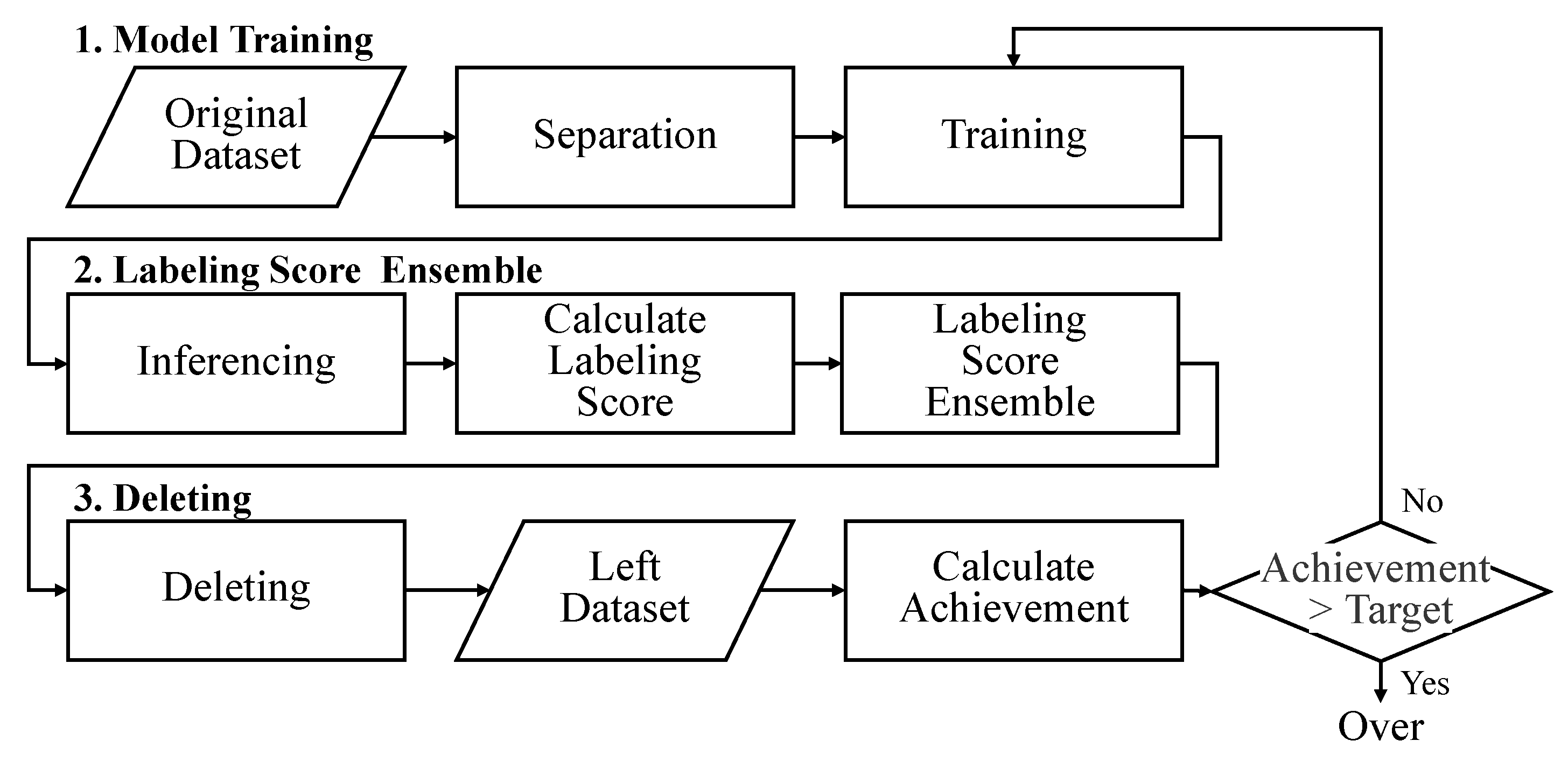
Figure 4.
Flowchart of the whitening data distribution process. This process involves three steps: calculating the diversity scores, whitening the data, and training the model. The diversity scores were derived from the class and bounding box size distributions. The whitening score, combining these with the , guides data reduction by prioritizing the data to be reduced. The model is then trained to determine the optimal reduction level.
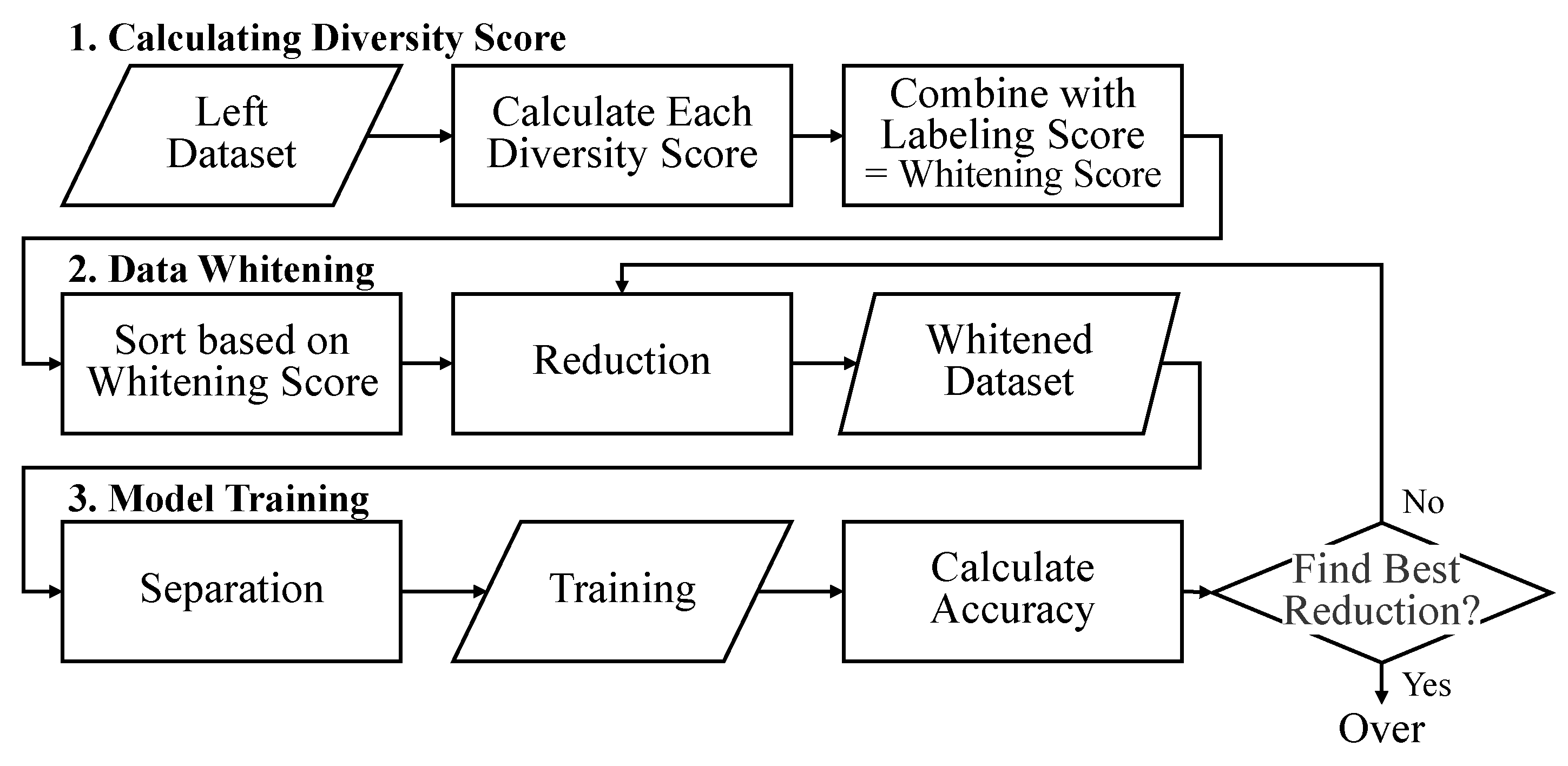
Figure 5.
Explain why LScores should be combined with whitening scores. Figure 5(a) shows an example of a high diversity score but a low E’LScore. Although they are rare classes, buses and bicycles have noisy labels. Figure 5(b) shows a low diversity score but a high LScore. It comprises of data with common objects but clean labels.
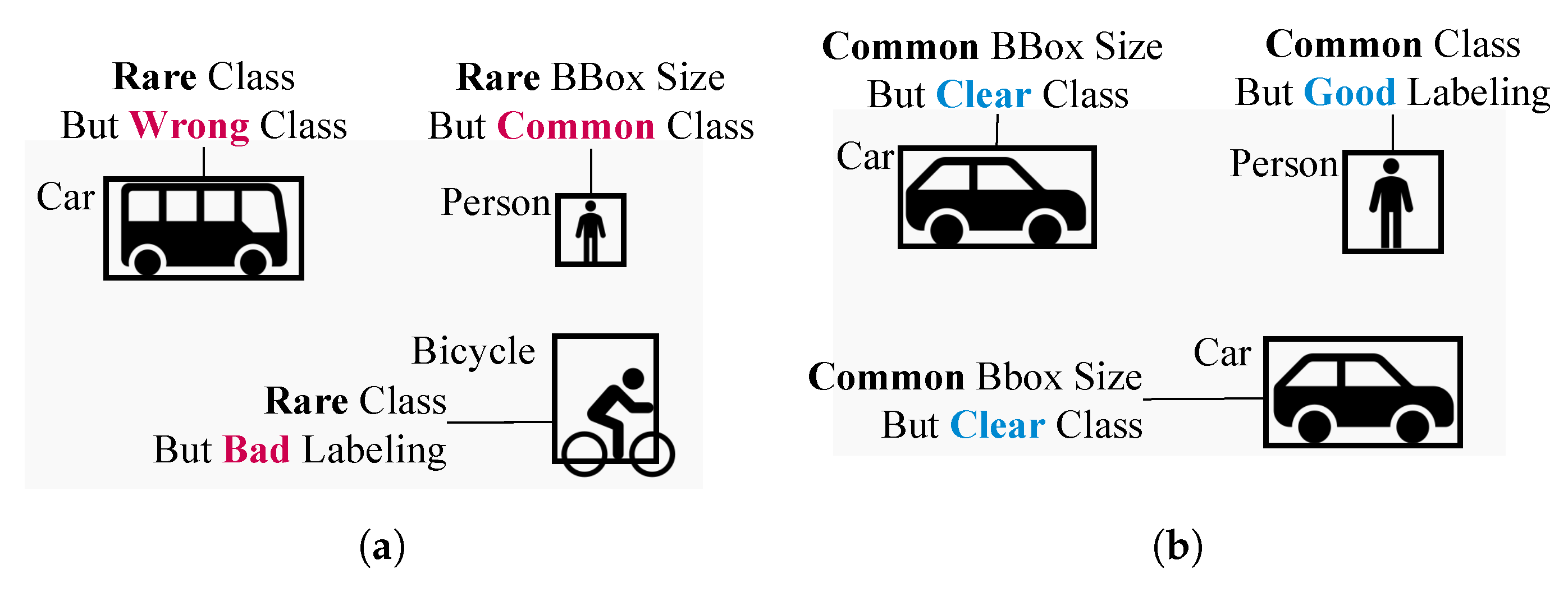
Figure 6.
Results from the deleting noisy labels module on the KITTI dataset. Figure 6(a) is an example of filtering out incorrect labels. Figure 6(b) shows that the module automatically found the inaccurate label. Figure 6(c) shows data with incorrect and missing labels.
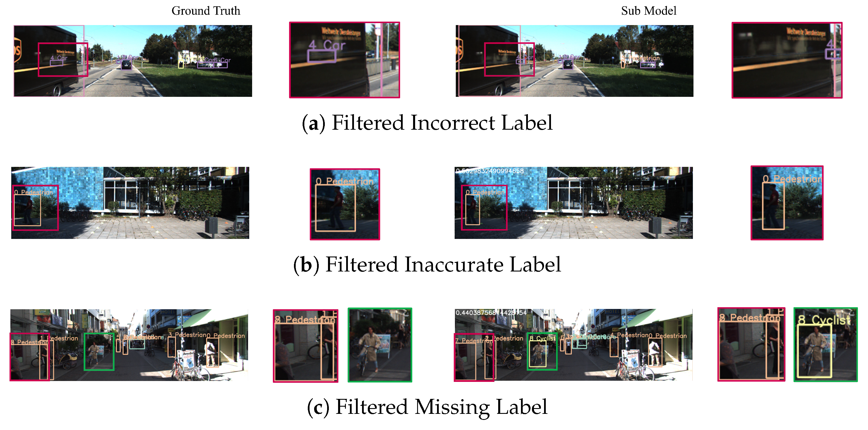
Figure 7.
Results of deleting noisy labels module on nuScenes dataset. The number of deleted data items in Tab. Table 2, the largest percentage of data was deleted. Figure 7(a) is an example of incorrect data. Figure 7(b) is an example of missing labels, and Figure 7(c) is an example of inaccurate data.
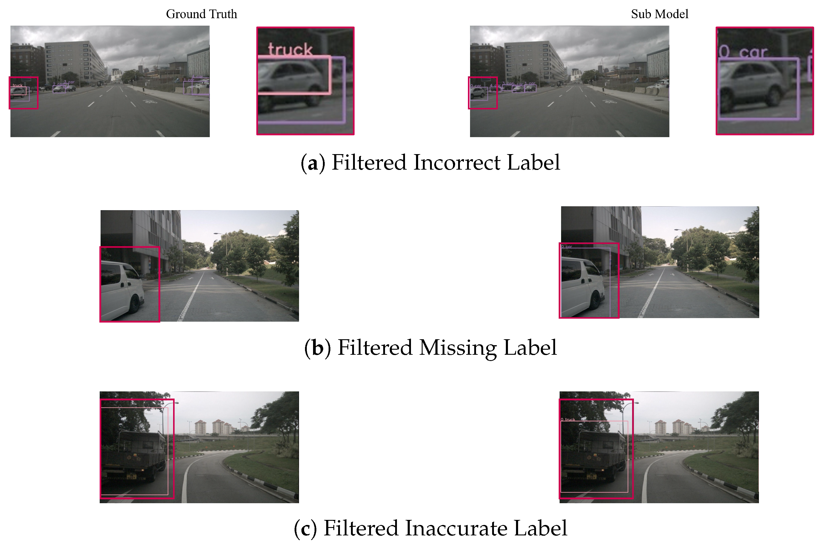
Figure 8.
The noise data were filtered using the ADVWC dataset. ADVWC contains severe weather data, and most objects are not clear. Figure 8(a) is an example of missing labeling. Figure 8(b) shows data with missing labels for small objects. Figure 8(c) is an example of incorrect data assigning different classes to objects.
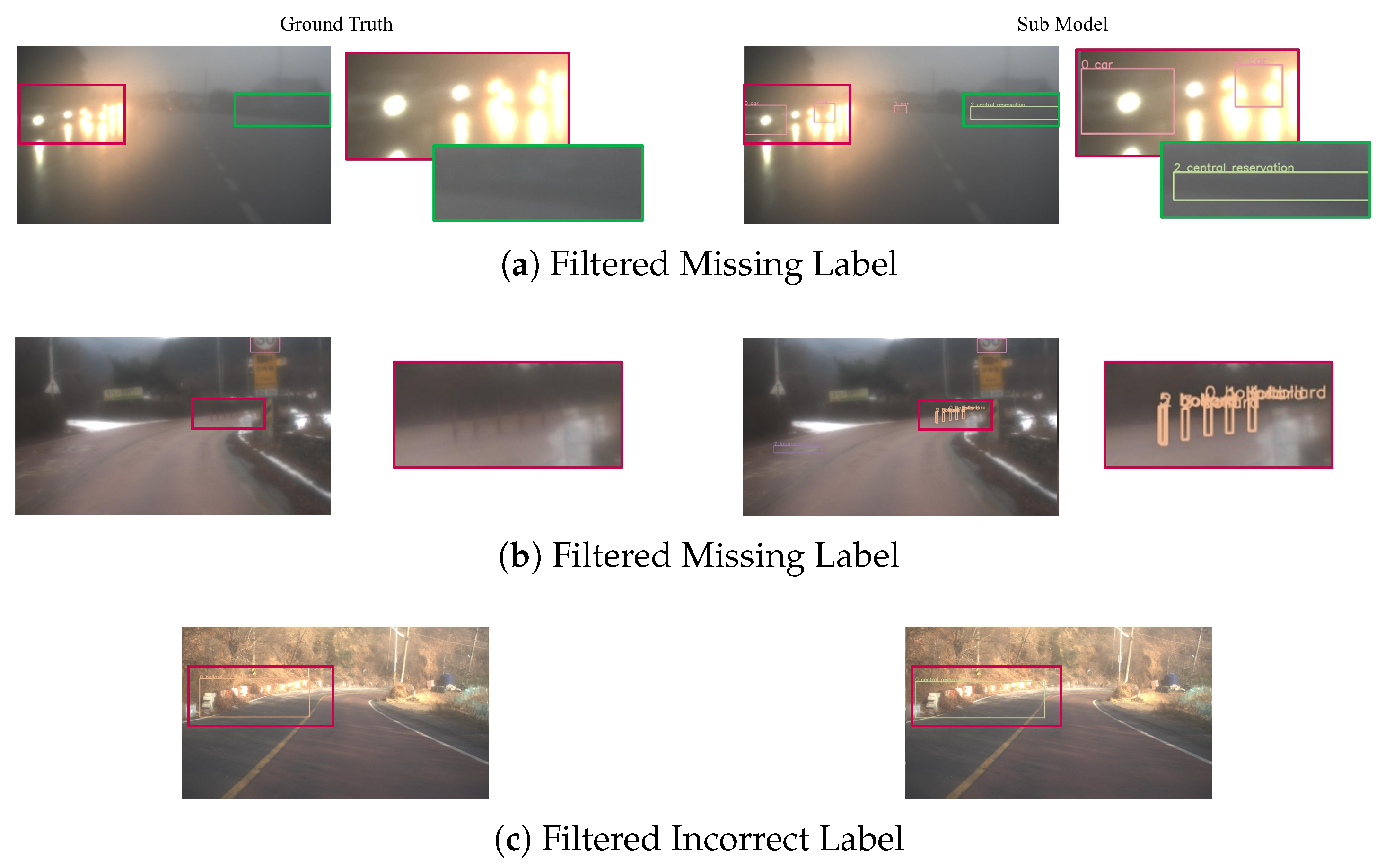
Figure 9.
Example of data filtered by noisy labels from the GECSSD dataset. Figure 9(a) is an example of damage. This results from the class being reversed in the processing and storage stage. Figure 9(b) is also filtered by damaged data. Figure 9(c) shows data with missing labels.
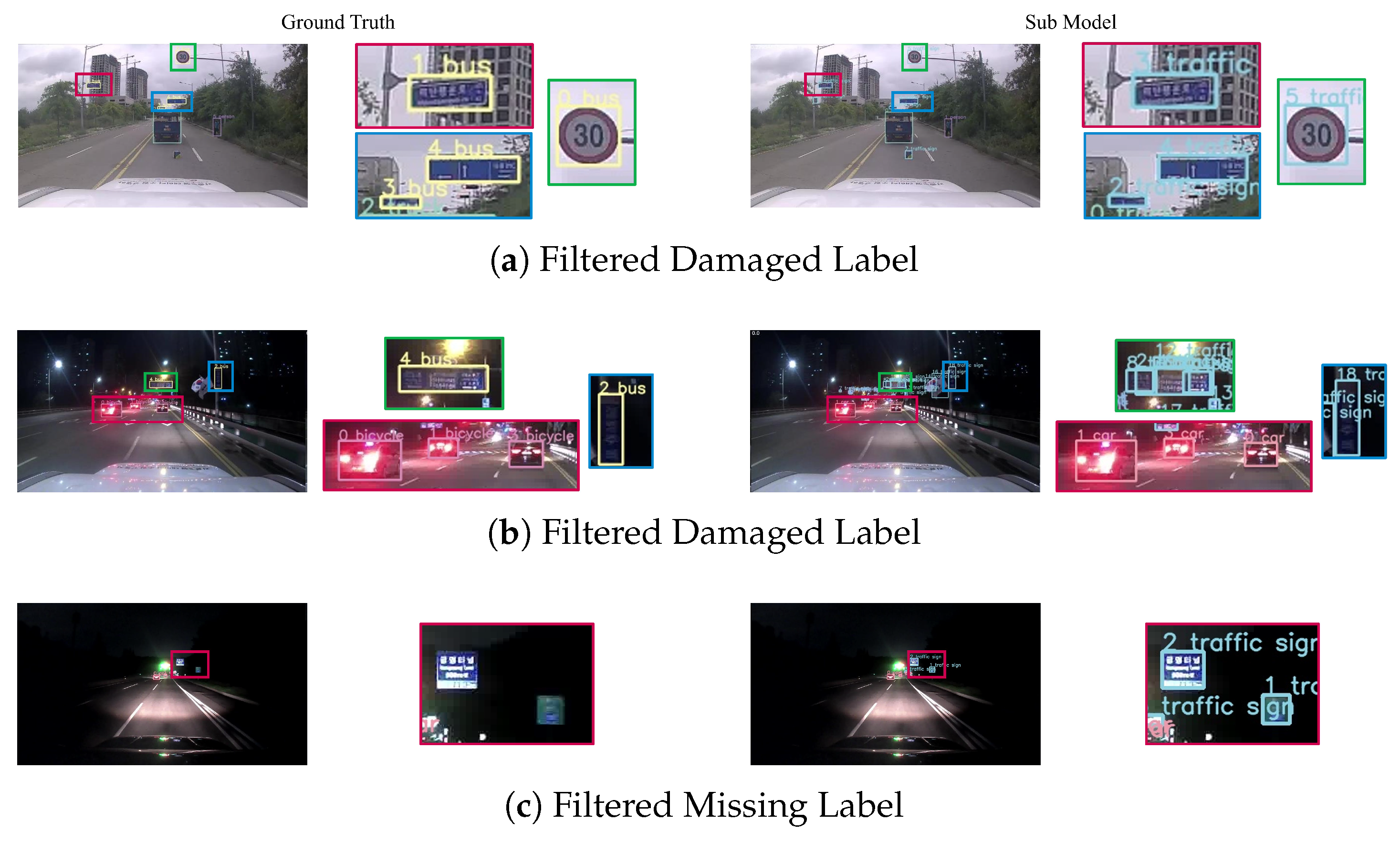
Figure 10.
Variations in the class distribution and bounding box sizes within the KITTI dataset resulting from the data distribution whitening module. The hatched circle represents the distribution before the module, and the colored circle represents the distribution after the module. Figure 10(a) shows that the distribution has been reduced to many cars. Figure 10(b) shows that the distribution of objects corresponding to 20% in the smallest size is the highest in the entire.
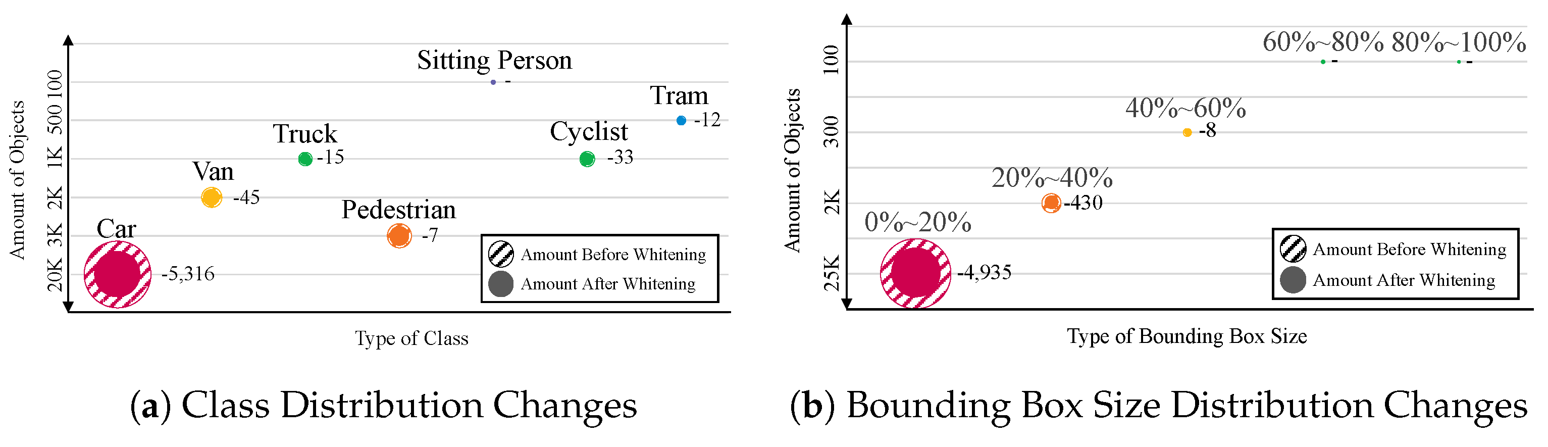
Figure 11.
Example of Waymo data excluded from training because of low whitening score. The Waymo dataset had the highest distribution of car objects, and the data for these objects were reduced.
Figure 11.
Example of Waymo data excluded from training because of low whitening score. The Waymo dataset had the highest distribution of car objects, and the data for these objects were reduced.
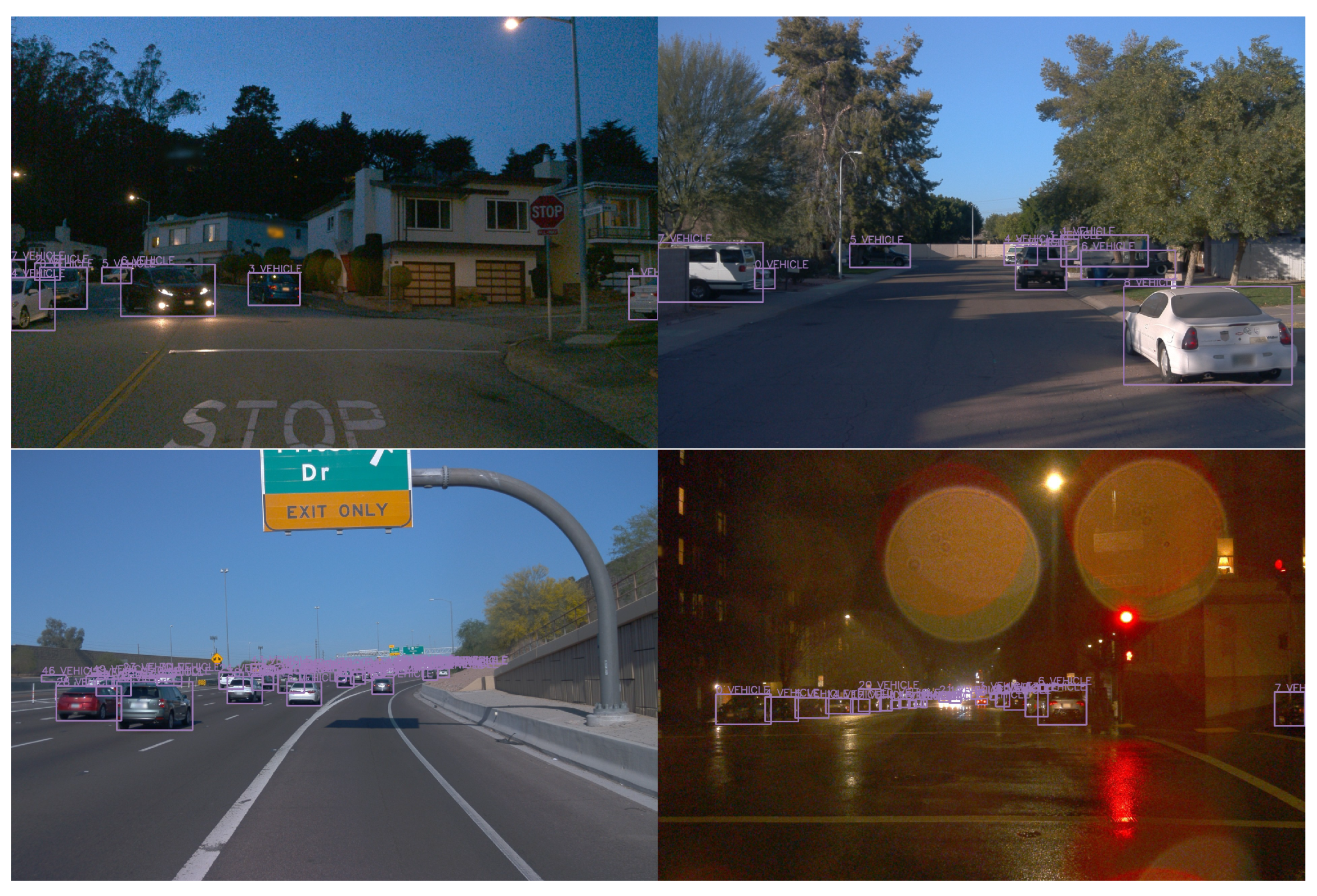
Figure 12.
nuScenes data with low priority owing to their low whitening score. In the nuScenes data, there were several objects in the order of pedestrians, cars, and barriers. These objects belong to a distribution with a small bounding box size. Even if a rare object exists, the data are included in the reduction process because of an inaccurate bounding box.
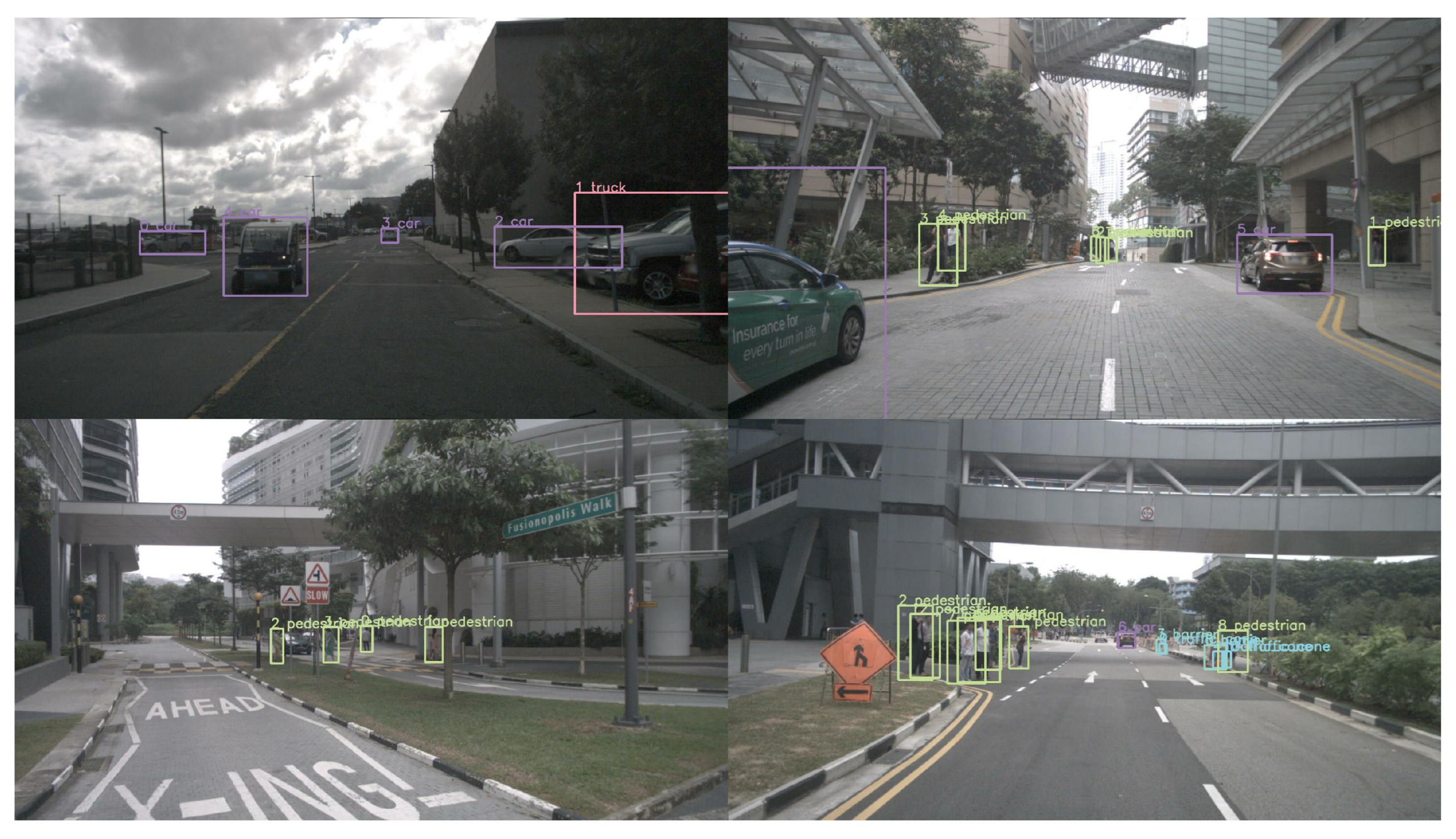
Figure 13.
Graph of class distribution and bounding box size distribution changes in nuScenes dataset. Data when performance was the highest. According to Figure 13(a), the inside of the circle is the number of reduced objects, which are reduced to pedestrian objects with the largest distribution. Figure 13(b) shows that the most objects have a size within 20%, and large objects are not included in the data reduction.
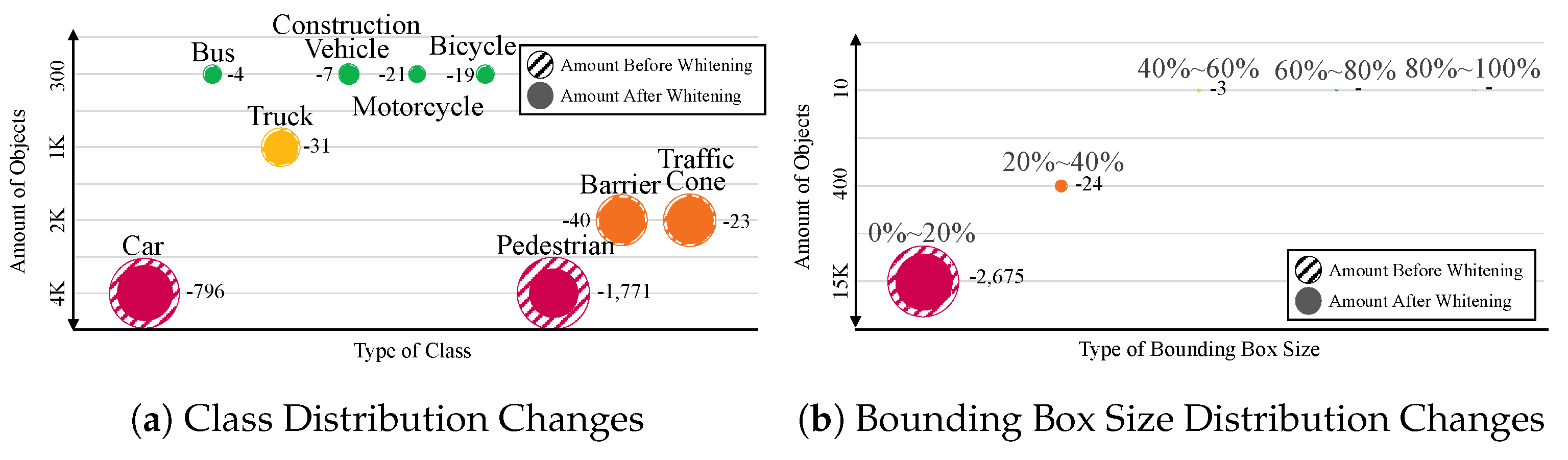

Table 1.
Comparison of the datasets used in the experiment.
| Dataset | Owner | Image Resolution |
Number of Images |
Number of Classes |
|---|---|---|---|---|
| KITTI | Karlsruhe Institute of Technology |
1242 × 375 | 7,481 | 7 |
| Waymo | Waymo LLC | 1920 × 1080 | 6,330 | 4 |
| nuScenes | nuTonomy | 1600 × 900 | 3,376 | 10 |
| RDID | Korea Automobile ResearchInstitute |
1280 × 720 | 48,025 | 26 |
| ADVWC | Korea Electronics Technology Institute |
1920 × 1080 | 57,612 | 23 |
| GECSD | Korea Transportation Safety Authority |
1920 × 1080 | 207,068 | 9 |
Table 2.
Results of Deleting Noisy Label on six datasets.
| Dataset | Iteration (Best) |
Accuracy Before |
Accuracy After |
Number of Data |
Number of Deleted Data |
|---|---|---|---|---|---|
| KITTI | 2 (1) | 65.62 | 65.64 (+0.02) | 7,481 | 410 (-5%) |
| Waymo | 1 (1) | 46.58 | 46.99 (+0.41) | 6,330 | 76 (-1%) |
| nuScenes | 3 (3) | 59.19 | 59.70 (+0.51) | 3,376 | 675 (-19%) |
| RDID | 3 (1) | 66.02 | 66.48 (+0.46) | 48,025 | 775 (-2%) |
| ADVWC | 3 (2) | 66.52 | 67.95 (+1.43) | 57,612 | 7,541 (-13%) |
| GECSD | 3 (3) | 58.65 | 59.95 (+1.30) | 207,068 | 22,914 (-11%) |
Table 3.
Results of the whitening data distribution on six datasets.
| Dataset | Reduction (Best) |
Accuracy Before |
Accuracy After |
Number of Data |
Number of Reduced Data |
|---|---|---|---|---|---|
| KITTI | 30% | 65.64 | 67.96 (+2.32) | 7,071 | 2,123 |
| Waymo | 20% | 46.99 | 47.15 (+0.16) | 6,254 | 1,251 |
| nuScenes | 30% | 59.70 | 62.59 (+2.89) | 2,701 | 805 |
| RDID | 20% | 66.48 | 66.40 (-0.08) | 47,250 | 9,450 |
| ADVWC | 20% | 67.95 | 68.05 (+0.10) | 50,071 | 10,015 |
| GECSD | 30% | 59.95 | 60.55 (+0.60) | 184,154 | 55,245 |
Disclaimer/Publisher’s Note: The statements, opinions and data contained in all publications are solely those of the individual author(s) and contributor(s) and not of MDPI and/or the editor(s). MDPI and/or the editor(s) disclaim responsibility for any injury to people or property resulting from any ideas, methods, instructions or products referred to in the content. |
© 2025 by the authors. Licensee MDPI, Basel, Switzerland. This article is an open access article distributed under the terms and conditions of the Creative Commons Attribution (CC BY) license (http://creativecommons.org/licenses/by/4.0/).
Copyright: This open access article is published under a Creative Commons CC BY 4.0 license, which permit the free download, distribution, and reuse, provided that the author and preprint are cited in any reuse.


