
Submitted:
02 April 2025
Posted:
04 April 2025
You are already at the latest version
Abstract
This paper presents an adaptive strategy to solve the formation control problem for a set of second-order agents with parametric uncertainty and nonlinearity. The strategy regards a group of agents where the nolinearities and uncertainties are represented by a linearly parametrised term, which allows us to consider non-identical agents. In order to ensure the collision-free motion of agents, we propose the use of a repulsive vector field component that is applied only when a pair of agents become nearer than a predefined minimum bound. Numerical simulations were carried out to show the effectiveness of the proposed scheme, first with a simplified example to verify the key features of the control law and a general case to illustrate the performance of the algorithm in a more complex scenario.
Keywords:
second-order systems
; uncertain systems
; adaptive control
; collision avoidance
1. Introduction
The study of Multi-Agent Systems (MAS) has increased significantly in the last decades as long as the development of technology has supported the application of these schemes in a wide variety of fields such as agriculture, patrolling, search and rescue, etc. [1,2,3,4,5]. In this kind of systems, a group of agents can perform tasks that for a single robot could be very difficult or even impossible. Among the main advantages of MAS are modularity, scalability, and decentralisation of tasks into the different members of the group. In this research area, there exist several issues that have been studied, e. g., formation control, synchronisation, path following, containment control, among many others, [6,7,8,9].
In the formation control problem, agents have to reach a specific relative position or form a desired geometric pattern. This spatial distribution could be specified by global positions, inter-agent distances or relative displacements, known as position-, displacement- and distance-based, respectively. In each mentioned case, depending on the type of robot, agents need different sensor and communication capabilities to achieve the desired goal, [10]. In a position-based scheme, communication between agents is not needed, and agents are supposed to have access to their global positions, allowing them to reach their desired location without any interaction with other members in the group. On the other extreme, distance-based strategies only specify desired distances among agents which, depending on the initial conditions and robot’s sensing accuracy, can lead to a translated or rotated formation. Displacement-based strategies, serving as a midpoint, enable enhanced performance by utilising various decentralisation levels to optimise the resources dictated by the chosen robot model. The mentioned approaches have been applied to different kinds of robots modelled by single or double integrators, unicycle robots, high-order linear systems, among others, and also considering a number of additional constraints such as input saturation, failing actuators, time-delay communication, parametric uncertainty, etc.
In order to enhance the applicability of a proposed algorithm, more general models should be used to represent a more real behaviour of a physical systems and the constraints imposed by the structure or the equipment in the selected robots, as the parametric uncertainty and nonlinearity. In [11], uncertain second-order systems are studied. The authors assumed that the parameters of each robot could be different but known. Strategies are proposed to achieve formation tracking of the desired formation under switching directed topologies. In [12], the authors proposed a distributed adaptive control strategy for distance-based formation and flocking control. Nonidentical second-order agents are considered, and global convergence to the desired formation and to the leader’s velocity is achieved. In [13], strategies for agents to achieve formation tracking control under a leader-follower scheme regarding constant and time-varying leader velocities. Estimators to compensate for the uncertainties were designed in conjunction with PI-like controllers using the stress matrix. The backstepping technique was applied in [14] to estimate not only the uncertain parameters of the neighbouring agents, but also the desired trajectory parameters when the agents do not have access to global information. Recently, an adaptive backstepping approach in combination with neural networks has been proposed to solve the optimal formation control problem in finite-time [15].
One of the most important issues in MAS when they are meant to be deployed in real applications is the collision avoidance between agents or against obstacles in dynamic environments. This issue has been studied using a number of approaches. In [16] avoidance functions with finite cutoff were designed and the avoidance control is given by the gradient of the potential functions. Distance and velocity information was taken into account in [17] to clearly identify the situation which can lead to a collisions to reduce the energy consumption and minimize the effect of the avoidance potential field on the formation maintenance. A learning-based strategy to solve the formation control problem with collision avoidance was proposed in [18] by combining neural networks and the artificial potential field Technique. In [19] a scheme based on neural networks and improved potential functions we proposed for second-order uncertain systems with disturbances. Recently, in [20] a fuzzy logic controller was proposed to solve the formation control problem for a group of unmanned aerial vehicles where the collision-free motion is guaranteed applying the artificial potential method.
In this paper, a solution to the formation control problem without collisions is proposed regarding a general uncertain model for second-order agents. The strategy regards a group of agents where the nolinearities and uncertainties are represented by a linearly parametrised term, which allows us to consider non-identical agents. We assume that the communication among agents is such that there exists, at least, a directed spanning tree. Inspired by an algorithm previously developed for first-order systems, we propose an extension for second-order systems by using a backstepping-like technique. Moreover, uncertainty and nonlinearity in the form of a parametrisable structure is added to each agent. This uncertain term is compensated by a local adaptive component in the control law.
To ensure the collision-free motion of agents, we propose the use of repulsive vector fields that is applied only when a pair of agents become nearer than a predefined minimum bound. These vector fields are designed using an unstable focus structure, in such a way that there do not exist undesired equilibria, that is, the agents do not get stuck at undesired configurations. This additional component of the control law is position- and velocity-based and is activated in a smooth way by using a bounded switching function.
In order to distinguish between the effect of local uncertainty and the influence of other surrounding agents, the adaptation law is only applied when there is no risk of collision, that is, each agent estimates its own parameters only when there are no other agents in its detection region. Otherwise, the agent retains the last estimated value of parameters and a repulsive vector field is enabled to guarantee the collision-free motion. When the conflict is solved and there is no threatening agents, the adaptation law is restarted taking the last save parameters values.
The remainder of the paper is organised as follows. In Section II, we review some important concepts on graph theory and recall some well-known lemmas. We formally state the problem in Section III and in Section IV we give our main contribution. Numerical simulations were carried out to show the performance of the proposed algorithms which results are presented in Section V. Finally, some conclusions and outlines for next stages of this research are listed in Section VI.
2. Preliminaries
In this Section we recall some important graph theory concepts as well as some lemmas that will be useful in the rest of the paper.
Communication among a group of agents is represented through a formation graph , which consists of a set of vertices representing the agents. The graph also includes a set of edges , where each edge indicates that agent receives information from agent . Here, is called the parent node and the child node. Furthermore, there is a set that contains constant vectors that specify the desired relative position of agent regarding its neighbours.
A formation graph is undirected if, for any , the reverse also holds, indicating bidirectional communication. In contrast, the graph is considered directed if does not imply . When a formation graph is neither solely directed nor undirected, it is classified as mixed. There is a path connecting the vertices and if there is a succession of edges as follows: , with . A directed tree is defined as a directed graph in which each node, except one, called the root, has a single parent. The root lacks a parent and has a direct path to all other nodes. A directed tree incorporating all nodes of a directed graph G is termed a directed spanning tree.
For a given graph G, its Laplacian matrix is expressed as
where the degree matrix is specified by , with representing the number of edges pointing to , for . Meanwhile, the adjacency matrix of G is defined as:
A function qualifies as a saturating function if it meets the following criteria:
- i)
- ,
- ii)
- for some ,
- iii)
- , for all , and
- iv)
- .
Conversely, a smooth switching function satisfies these conditions:
- i)
- if ,
- ii)
- if ,
- iii)
- if ,
- iv)
- ,
where .
Definition 1.
The system
is said to be input-to-state stable (ISS) if there exist a class function β and a class function γ such that for any initial state and any bounded input , the solution exists for all and satisfies
Lemma 1
Lemma 2
Lemma 3
(Barbalat’s Lyapunov-Like Lemma[22]). If a scalar function satisfy the following conditions
- is lower bounded
- is negative semi-definite
- is uniformly continuous in time
then, as .
3. Problem Statement
Consider the set consisting of agents moving on a plane. Each agent is represented by a second-order model with uncertainties given by
where , and are the position, velocity and acceleration of the i-th agent, respectively. Let be a matrix of known bounded nonlinear smooth velocity- and/or time-dependent functions and a vector of unknown parameter, that is, the agents are not identical. It is assumed that each robot can determine for all times its own relative position and velocity with respect to a specific subset of robots , which is defined according to the formation graph G. Hence, the desired position is defined as
where is the cardinality of and are constant vectors that define the geometrical patter to be reached by the agents. Moreover, each agent can detect and measure the relative position and velocity of all agents within a radius D, defined as and called the sensing region. In the same way, we define the collision region , where d is the minimum safety distance between any pair of agents.
The control objective is to design distributed controllers , , for such that
- i)
- The agents achieve the desired formation by reaching their desired positions, that is,
- ii)
- The agents avoid collision by remaining at a distance greater than or equal to the safety distance d;
- iii)
- Once the desired formation is reached, the whole pattern does not move from its current location any more, i. e., , .
Error dynamics
As stated in the control objective the agents are required to achieve a desired formation, then we define the position error as , whose dynamics is
In view of (7a)-(7b) and the fact that the formation should be static once it is achieved, the whole system could be stacked as
where is the Laplacian matrix, is the identity matrix, ⊗ denotes the Kronecker product, , , , , , , with .
4. Control Design
In this Section we present the design of an adaptive control law to locally compensate for the uncertainties in the model of agents. Once the convergence to the desired formation is guaranteed, we derive conditions to force the agents to remain separated from one another by applying a complementary repulsive component to the control law, which consists in regarding any other agent as an unstable focus structure to generate a repulsive vector field that ensures the collision-free motion.
4.1. Adaptive Formation Control
For our purposes, we begin by designing an adaptive strategy based on the basic result proposed in [23]. Indeed, using a bounded control input with the form , being a saturation function and a positive constant, the closed-loop system in vector form is
where , is asymptotically stable. Now, if we add and subtract the right hand term in (12) to the position errors (11a), we have
where the auxiliary variable has been defined and whose dynamics is given by
or equivalently,
If the parameters were known, the control input could be selected as
with . Then, the closed-loop system become
which was shown in [24] to be asymptotically stable by using the cascades system approach and implying that agents reach the desired pattern and their velocities become zero once the formation is achieved.
On the other hand, if the parameters in are not exactly known, the control law should be implemented using the estimated parameters , that is
Then, the dynamics of the auxiliary variable is now
where the estimation error is defined as .
Theorem 1.
Consider the system (11a)-(11b) and the control law (19) with μ and λ being positive constants. Assume that the formation graph contains at least a directed spanning tree. Then, applying the adaptation law
where is a positive definite matrix in , the mobile agents reach the desired formation while compensate for their local uncertainty. Moreover, once the desired pattern is achieved, the velocity of the formation becomes zero.
Proof.
Applying the control law (19) the closed-loop system is
Using the cascaded system approach it can be shown that (22) is input-to-state stable. Then it is enough to verify that the subsystem (23) is asymptotically stable to ensure that the whole system is asymptotically stable [21]. Consider the next Lyapunov candidate function
Then, the corresponding time derivative is
which can be written as
Then, applying the adaptation law (21) and in view that , the Lyapunov candidate function reduces to
which is semidefinite negative and implies , that is, and are bounded. Now, if we use the second time derivative to verify the uniform continuity of we have
Since we assumed w to be bounded and we have shown that and are bounded, then is bounded as well, which implies that is uniformly continuous. Hence, by direct application of Barbalat’s lemma, we can conclude that as . Then, under the cascaded system approach, (22) is asymptotically stable, which implies that and as , which means that agents reach the desired formation and the velocity becomes zero. This completes the proof. □
4.2. Collision Avoidance Strategy
Once the convergence to the desired formation has been shown, it is necessary to design a complementary strategy to guarantee collision-free motion by ensuring that the agents remain at a minimum predefined distance. Similarly to the last subsection, we start with a proposal for a previously studied first-order system [23] that ensures collision-free performance. The basic strategy is given by
where the second right-hand term provides a repulsive action in the form of an unstable focus structure provided by the matrix
The repulsive component is activated in a smooth way using the distance-based switching function which takes values between 0 and 1 as the distance between the and the agent goes from D to d; The parameter is a positive constant that guarantees collision-free motion for values ([25]). If we apply (26), the position error dynamics (11a) becomes
where is a matrix which depends on the distance between every pair of agents and models the conflicts among agents. Its general form is
Remark 1.
It is important to note that (28) is reduced to (12) when the agents are far away from each other, that is, there is no risk of collision between any pair of agents. Then, the second right-hand term in (28) could be considered as a vanishing perturbation term at the origin of the stable dynamics (12).
Assumption A1.
The intended configuration is specified such that the separation between any two agents exceeds a predefined minimum d, ensuring that no agent falls within another’s sensing range. In the same way, we assume that under the initial conditions, there exists no risk of collision between agents, that is, , .
If we proceed as in the previous subsection, we can define an auxiliary variable such that
where and . This auxiliary variable has a dynamics
At this point, we need to notice that, indeed, the repulsive component of the control law imposes changes in the trajectory followed by the agents. Then, to distinguish the effect of the repulsive vector field provoked by the presence of surrounding agents from the local parametric uncertainty, the adaptation law is just applied when there exists no risk of collision, that is, when no agents are detected into the sensing region. Otherwise, the control law regarding the repulsive component is implemented using the last estimated parameters until the conflict between agents is solved. Therefore, the control input can be chosen as
where and is the last estimation of the vector , giving priority to the safety motion over the formation control objective. Once the conflict between agents has been solved, the agents restart the parameter adaptation. We are now ready to state our main result.
Theorem 2.
Consider the closed-loop system (Section 3)-(32) along with definitions (27), (29). Consider that the formation graph contains at least a directed spanning tree, and Assumption 1 holds. If there is no risk of collision among agents, the control law (32) becomes (19) where the estimated vector is obtained from the adaptation law
where is a definite positive matrix in . On the other hand, if there is a pair of agents that enter their sensing region, the control law (32) is applied using which is the last estimated value of θ. Then, mobile agents are able to resolve any conflict between them and reach the desired formation while compensating for their local uncertainty. Moreover, the velocity of the formation becomes zero once the formation pattern has been achieved.
Proof.
As mentioned, when agents are far enough from each other, the applied control law is (19) which corresponds to Theorem 1. Then, it is necessary to show that when agents are at risk of collisions, the strategy (32) is able to effectively solve conflicts to prevent collisions. In closed-loop we have
where is the estimation error which is constant while the collision avoidance component is applied. Since there is not adaptation law, we just use a single quadratic Lyapunov function
whose time-derivative is
If is bounded by , then
which implies that when . Then, (34) is Input-to-State stable, which in combination with ensures that . As a result,
As mentioned before, is a vanishing perturbation at the origin of the subsystem, then which finally means that . In summary, the agents reach the desired formation while they avoid collisions. In addition, the whole formation remains static after it is achieved. □
5. Simulation Results
In this Section we present the results of numerical simulations carried out to show the performance of the proposed scheme. The first one consists of a reduced system composed of only two agents and is meant to illustrate as clearly as possible the main features of our scheme. Then, a second simulation was developed with the objective of verifying the performance of our strategy in a more complex scenario composed of four agents.
Two-Agents System with Bidirectional Communication
Consider a pair of second-order agents in the plane with linearly parameterised uncertainty,
with , . Assume there exists bidirectional communication between the agents and the objective is to them be located at some specific position with respect to each other. This displacement is given by the constant vector . The initial conditions were , , , and . The function used to apply the repulsive component is given by
with values and . As we can see in Figure 1, the switching function is fully activated for distances of about metres.
It is important to mention that the initial positions were selected to provoke an imminent risk of collision. In the same way, initial estimated parameters were assumed to be zero, which means that there is no prior knowledge of real values. The results of this first simulation are shown in Figure 2 where, in the upper left corner, the trajectories of the agents in the plane are shown. It is clear that the agents reach the desired relative desired positions while they avoid the collision successfully and do not get stuck even when applying the same vector field. Moreover, they exhibit a smooth behaviour given by the transition and saturation functions involved in the control law. In the upper right corner, the distance between the agents is depicted. As can be seen, the distance never decreases more than the safety distance. The magnitudes of the velocities are shown in the lower left corner, while the estimated parameters are depicted in the lower right corner. The period from 6 to 8 seconds in which the estimated parameters are constant corresponds to the time at which the parameter estimation is frozen to attend the collision avoidance control.
Four-Agents System with General Communication Topology
As a second example, consider a set of four agents whose communication graph is shown in Figure 3. The geometric pattern to be formed is defined by the constant vectors , , , , . For this simulation, we considered agents with a similar local uncertain term than in the last example, i. e.,
for , and for we have
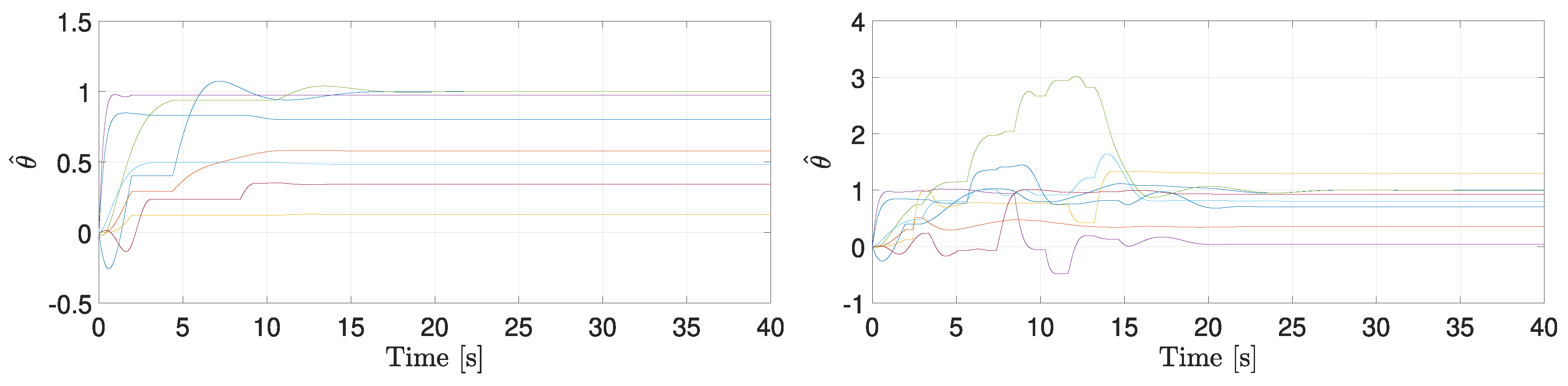
For the switching function, parameters were and which give a fully activation of the repulsive force about 3 metres. The initial conditions were , , , , , , , . In Figure 4, Figure 5, Figure 6 and Figure 7 the results of this simulation are shown, comparing the behaviour of the system under the control laws with and without repulsive vector fields on the left and right, respectively. Figure 4 illustrates the trajectories of the agents in the plane, verifying that in both cases the desired formation is reached. However, in Figure 5 the distances between each pair of agents are shown and it is clear that when applying the avoidance component the agents remain at a greater distance than the safety radius. On the other hand, Figure 6 shows that in both cases the velocity of the resulting formation becomes zero, but the settling time is larger if the collision avoidance strategy is applied. Finally, in Figure 7 local estimated parameters are depicted. In this case, when there exists a conflict between any pair of agents, the estimation law is stopped, and the last estimated value is used to apply the control input. When agents get far from each other, the adaptation law is re-established.
6. Conclusions
In this paper, we have proposed an adaptive strategy to solve the formation control problem for a set of second-order agents with parametric uncertainty. Repulsive vector fields with unstable focus structure were used to avoid collisions among agents by keeping them at a distance greater than or equal to a predefined minimum bound. These vector fields are such that the agents do not get stuck in any undesired configuration while repelling each other. An adaptation law is applied only when there is no risk of collisions, while the controller keeps and uses the last estimated parameter into the control law until the conflict between agents is solved and then the adaptation continues in order to ensure the desired position is reached despite of the uncertainty. Simulations were carried out to illustrate the performance of the proposed algorithm, which shows the effectiveness of the approach. As the next step, time-varying formation tracking, connectivity preservation, and communication delay could be considered, as well as experimental validation.
Author Contributions
Conceptualization, J.F.F.-R. and J.D.A; methodology, All authors; software, J.F.F.-R.; validation, J.F.F.-R.; formal analysis,J.F.F.-R. and J.D.A; investigation, All authors; writing—original draft preparation, All authors; writing—review and editing, J.F.F.-R. and J.D.A; All authors have read and agreed to the published version of the manuscript.
Conflicts of Interest
The authors declare no conflicts of interest.
Abbreviations
The following abbreviations are used in this manuscript:
| MAS | Multi-Agent Systems |
| ISS | Input-to-State Stable |
References
- Jawhar, I.; Mohamed, N.; Kesserwan, N.; Al-Jaroodi, J. Networking Architectures and Protocols for Multi-Robot Systems in Agriculture 4.0. In Proceedings of the 2022 IEEE International Systems Conference (SysCon), 2022, pp. 1–6. [CrossRef]
- Huang, L.; Zhou, M.; Hao, K.; Han, H. Multirobot Cooperative Patrolling Strategy for Moving Objects. IEEE Transactions on Systems, Man, and Cybernetics: Systems 2023, 53, 2995–3007. [CrossRef]
- Noh, D.; Choi, J.; Choi, J.; Byun, D.; Kim, Y.; Kim, H.R.; Baek, S.; Lee, S.; Myung, H. MASS: Multi-Agent Scheduling System for Intelligent Surveillance. In Proceedings of the 2022 19th International Conference on Ubiquitous Robots (UR), 2022, pp. 252–257. [CrossRef]
- Abusalama, J.; Alkharabsheh, A.R.; Momani, L.; Razali, S. Multi-Agents System for Early Disaster Detection, Evacuation and Rescuing. In Proceedings of the 2020 Advances in Science and Engineering Technology International Conferences (ASET), 2020, pp. 1–6. [CrossRef]
- Queralta, J.P.; Taipalmaa, J.; Can Pullinen, B.; Sarker, V.K.; Nguyen Gia, T.; Tenhunen, H.; Gabbouj, M.; Raitoharju, J.; Westerlund, T. Collaborative Multi-Robot Search and Rescue: Planning, Coordination, Perception, and Active Vision. IEEE Access 2020, 8, 191617–191643. [CrossRef]
- Olfati-Saber, R.; Fax, J.A.; Murray, R.M. Consensus and Cooperation in Networked Multi-Agent Systems. Proceedings of the IEEE 2007, 95, 215–233. [CrossRef]
- Chung, S.J.; Slotine, J.J.E. Cooperative Robot Control and Concurrent Synchronization of Lagrangian Systems. IEEE Transactions on Robotics 2009, 25, 686–700. [CrossRef]
- Mastellone, S.; Stipanović, D.M.; Graunke, C.R.; Intlekofer, K.A.; Spong, M.W. Formation Control and Collision Avoidance for Multi-agent Non-holonomic Systems: Theory and Experiments. The International Journal of Robotics Research 2008, 27, 107–126. [CrossRef]
- Abhijith, U.P.; Thomas, S. Cyclic Pursuit of mobile robots: A linear approach. In Proceedings of the 2017 IEEE International Conference on Signal Processing, Informatics, Communication and Energy Systems (SPICES), 2017, pp. 1–5. [CrossRef]
- Oh, K.K.; Park, M.C.; Ahn, H.S. A survey of multi-agent formation control. Automatica 2015, 53, 424–440.
- Xiang, J.; Li, Y.; Dong, X.; Li, Q.; Ren, Z. Time-varying formation tracking for second-order multi-agent systems with switching directed topologies. Information Sciences 2016, 369, 1–13. [CrossRef]
- Zou, Y.; Wen, C.; Guan, M. Distributed adaptive control for distance-based formation and flocking control of multi-agent systems. IET Control Theory and Applications 2019, 13, 878–885. [CrossRef]
- Zhi, H.; Chen, L.; Li, C.; Guo, Y. Leader-Follower Affine Formation Control of Second-Order Nonlinear Uncertain Multi-Agent Systems. IEEE Transactions on Circuits and Systems II: Express Briefs 2021, 68, 3547–3551. [CrossRef]
- Cheng, X.; Huang, J.; Gao, T.; Wang, S.; Zhang, M. Distributed adaptive control of mobile robots with unknown parameters. IEEE, 5 2023, pp. 2624–2629. [CrossRef]
- Zhang, J.; Fu, Y.; Fu, J. Adaptive Finite-Time Optimal Formation Control for Second-Order Nonlinear Multiagent Systems. IEEE Transactions on Systems, Man, and Cybernetics: Systems 2023, 53, 6132–6144. [CrossRef]
- Mondal, A.; Bhowmick, C.; Behera, L.; Jamshidi, M. Trajectory Tracking by Multiple Agents in Formation With Collision Avoidance and Connectivity Assurance. IEEE Systems Journal 2018, 12, 2449–2460. [CrossRef]
- Pang, Z.H.; Zheng, C.B.; Sun, J.; Han, Q.L.; Liu, G.P. Distance- And velocity-based collision avoidance for time-varying formation control of second-order multi-agent systems. IEEE Transactions on Circuits and Systems II: Express Briefs 2021, 68, 1253–1257. [CrossRef]
- Mu, C.; Peng, J. Learning-Based Cooperative Multiagent Formation Control With Collision Avoidance. IEEE Transactions on Systems, Man, and Cybernetics: Systems 2022, 52, 7341–7352. [CrossRef]
- Yang, Y.; Liu, Q.; Tan, H.; Shen, Z.; Wu, D. Collision-Free and Connectivity-Preserving Formation Control of Nonlinear Multi-Agent Systems with External Disturbances. IEEE Transactions on Vehicular Technology 2023, 72, 9956–9968. [CrossRef]
- Yu, Y.; Chen, C.; Guo, J.; Chadli, M.; Xiang, Z. Adaptive Formation Control for Unmanned Aerial Vehicles With Collision Avoidance and Switching Communication Network. IEEE Transactions on Fuzzy Systems 2024, 32, 1435–1445. [CrossRef]
- Khalil, H.K. Nonlinear systems; 3rd ed.; Prentice-Hall: Upper Saddle River, NJ, 2002.
- Slotine, J.; Li, W. Applied Nonlinear Control; Prentice-Hall International Editions, Prentice-Hall, 1991.
- Flores-Resendiz, J.F.; Aranda-Bricaire, E. A General Solution to the Formation Control Problem Without Collisions for First-Order Multi-Agent Systems. Robotica 2020, 38, 1123–1137. [CrossRef]
- Flores-Resendiz, J.F.; Avilés, D.; Aranda-Bricaire, E. Formation Control for Second-Order Multi-Agent Systems with Collision Avoidance. Machines 2023, 11. [CrossRef]
- Flores-Resendiz, J.F.; Aranda-Bricaire, E.; González-Sierra, J.; Santiaguillo-Salinas, J. Finite-Time Formation Control without Collisions for Multiagent Systems with Communication Graphs Composed of Cyclic Paths. Mathematical Problems in Engineering 2015, 2015, 1–17. [CrossRef]
Figure 1.
Switching function. The parameters and ensure a sensing region radius of about metres and an avoidance safety distance of about metres.
Figure 1.
Switching function. The parameters and ensure a sensing region radius of about metres and an avoidance safety distance of about metres.
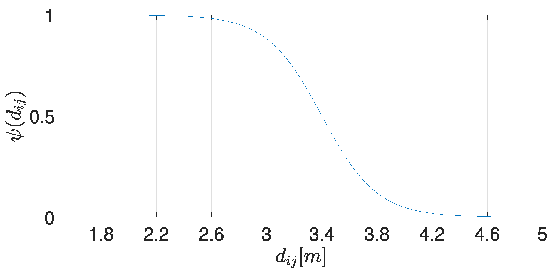
Figure 2.
Trajectories of the agents on the plane.
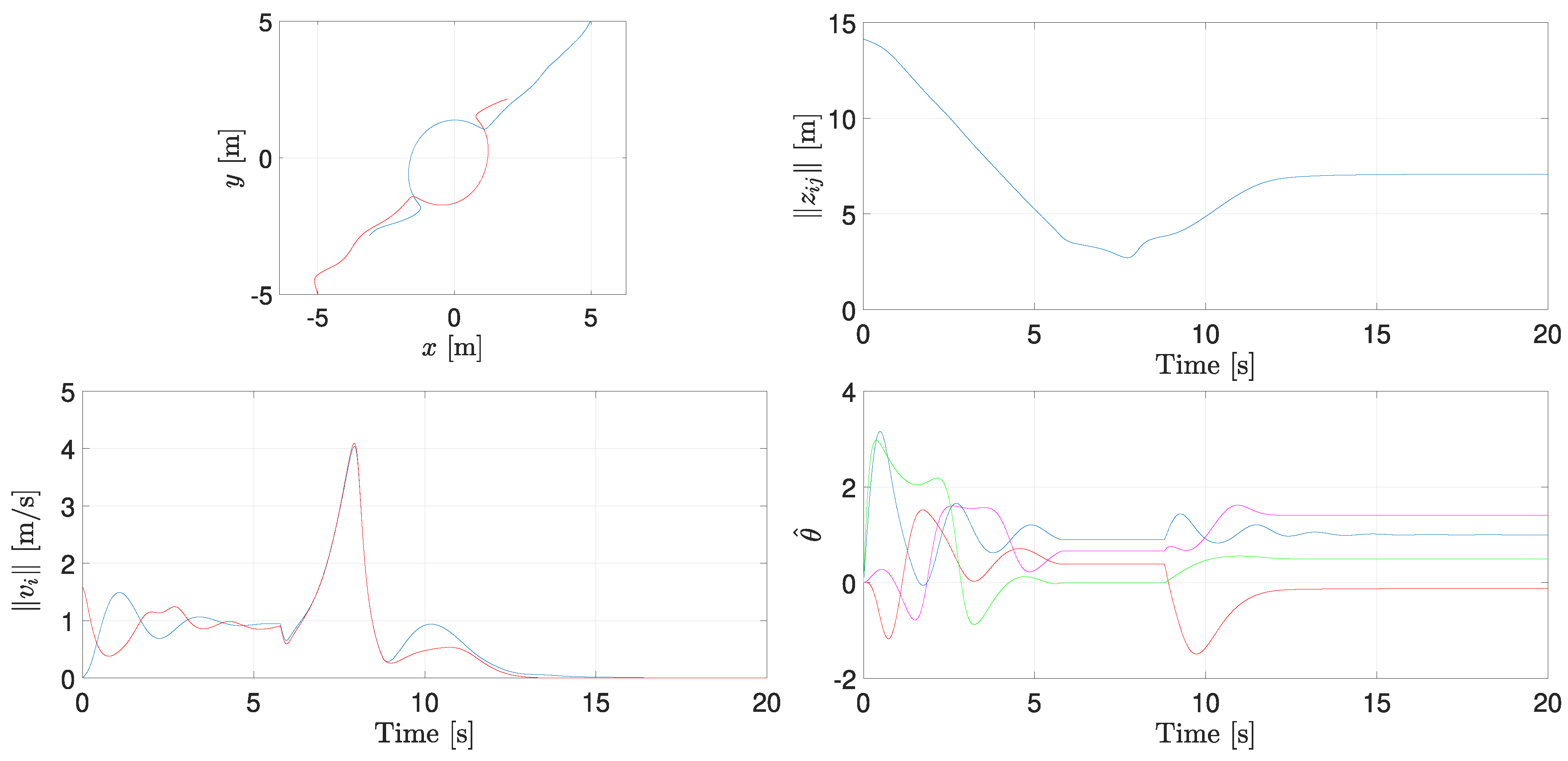
Figure 3.
Desired formation for the four-agent’s system.
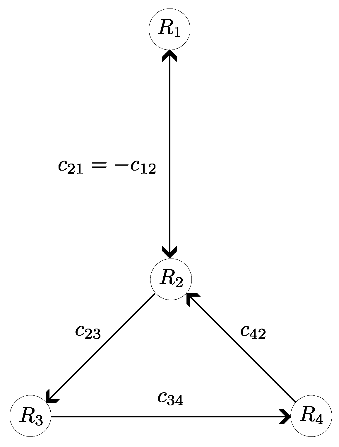
Figure 4.
Trajectories of agents in the plane without collision avoidance component (left) and applying the repulsive component (right).
Figure 4.
Trajectories of agents in the plane without collision avoidance component (left) and applying the repulsive component (right).
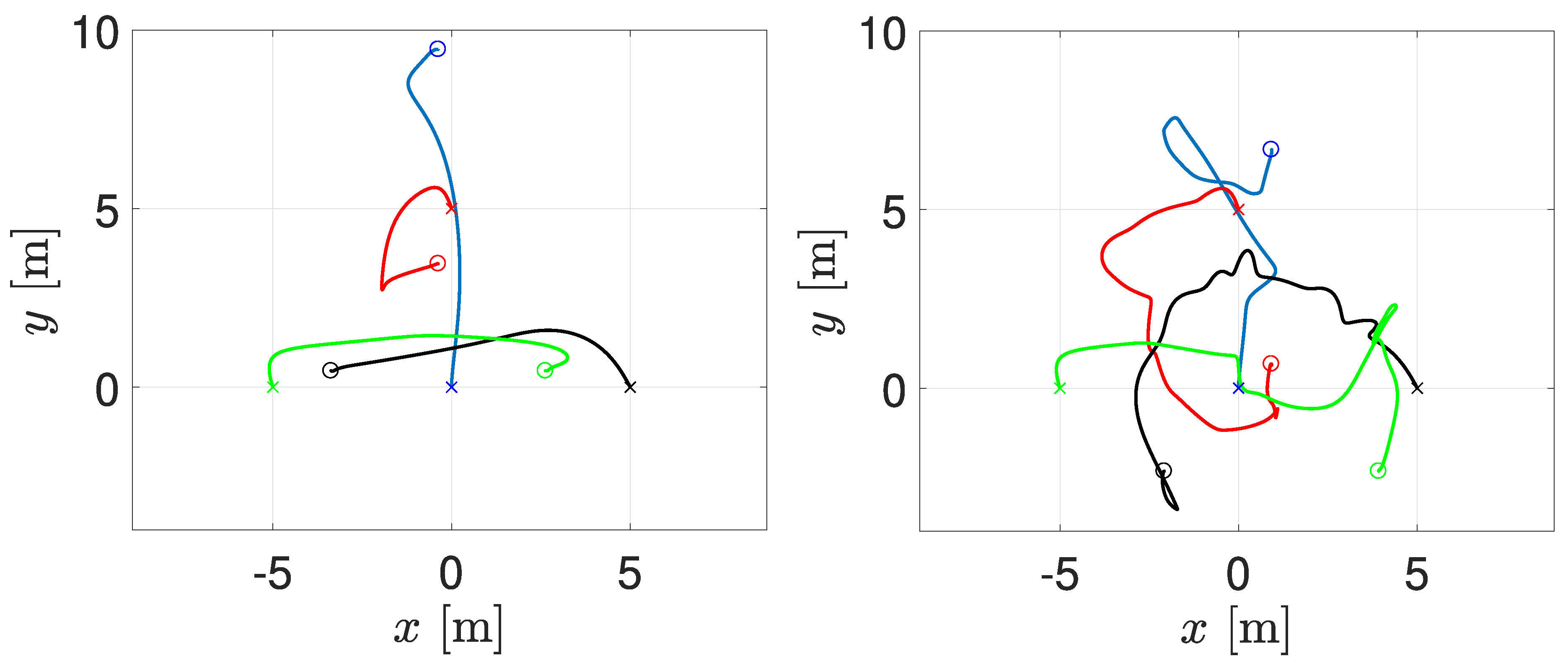
Figure 5.
Trajectories of the agents on the plane.
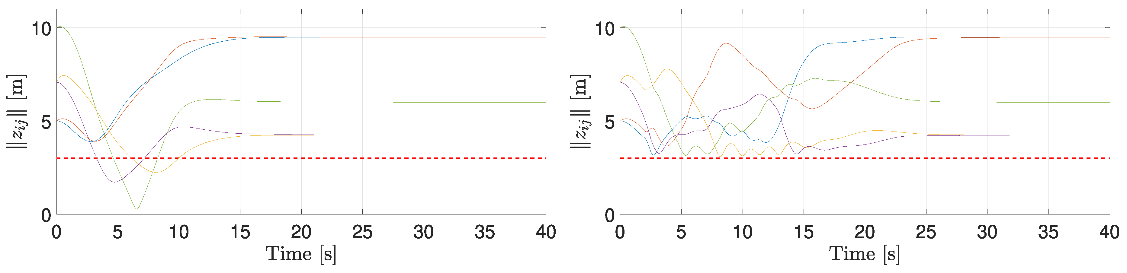
Figure 6.
Trajectories of the agents on the plane.
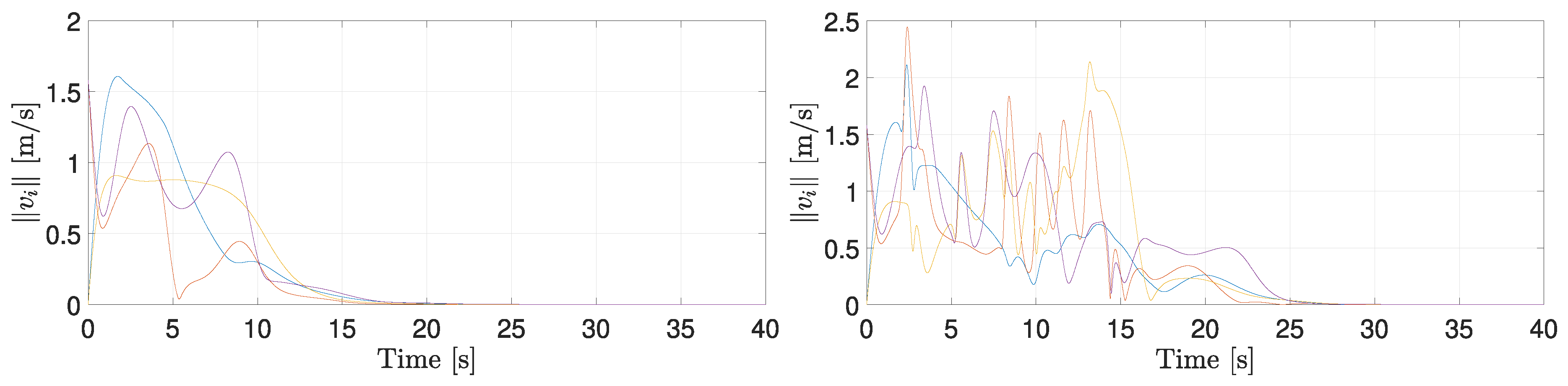
Figure 7.
Trajectories of the agents on the plane.
Disclaimer/Publisher’s Note: The statements, opinions and data contained in all publications are solely those of the individual author(s) and contributor(s) and not of MDPI and/or the editor(s). MDPI and/or the editor(s) disclaim responsibility for any injury to people or property resulting from any ideas, methods, instructions or products referred to in the content. |
© 2025 by the authors. Licensee MDPI, Basel, Switzerland. This article is an open access article distributed under the terms and conditions of the Creative Commons Attribution (CC BY) license (http://creativecommons.org/licenses/by/4.0/).
Copyright: This open access article is published under a Creative Commons CC BY 4.0 license, which permit the free download, distribution, and reuse, provided that the author and preprint are cited in any reuse.


