
Submitted:
07 April 2025
Posted:
07 April 2025
Read the latest preprint version here
Abstract
The objective is to show that the known features of global average sea-level over the last 120,000 years can be accounted for by eleven periodic functions associated with planetary orbits – the hypothesis. The method shows that proxy data for relative global average sea-level during the last glacial cycle, with errors measured in meters, and a modern sea-level reconstruction based on tide gauges, with errors measured in millimeters, are accurately fit using these periods and a single constant. The eleven periods, sine and cosine for each, and constant correspond to twenty-three functions. Reasons for including each period are provided. The fit predicts a maximum in global average sea-level on date 9,726 with elevation 12 meters above the 1930 level. Reasonable variations of the input data also predict a maximum in global average sea-level between years 9,726 and 12,605.
Keywords:
sea-level
; orbital-periods
; projected sea-level rise
1. Introduction
The objective is to show that the known features of global average sea-level can be accounted for by eleven periodic functions associated with planetary orbits – the hypothesis. The method will be to show that proxy data for relative sea-level during the last glacial cycle and a modern sea-level reconstruction are fit accurately using these periodic functions. The modern sea-level reconstruction has errors measured in millimeters while the Proxy data errors are measured in tens of meters. Figure 1 gives an early look at the fit.
This analysis begins by fitting three modern global average sea level (GASL) reconstructions, J-fit, C-fit, and D-fit, to establish that there exists an approximate sixty-year periodic variation in all three, see Figure 2, which corresponds to one of the periods associated with planetary motion. For these modern reconstructions, spanning 200 years or less, the initial background change in GASL will be represented by a cubic function of time. Later, when fitting 250,000 years of information this background variation will be determined by longer period functions associated with planetary orbits rather than polynomials.
An approximate sixty-year periodic variation in sea- level has been suggested by several authors, Jevrejeva [11], Chambers [3], Kalenda [14]. Recent information on sea-level is available from satellite measurements. However, early sea-level information (from 1800 to before 1993) comes from tide gauge measurements. Global average sea-level from tide gauges is a difficult quantity to measure since it is influenced by multiple factors. Some of these factors actually change sea-level itself while others change the elevation of measurement stations.
Proxy information has been used to approximate sea-level back through the last glacial period [8] and beyond [21]. This data will be used to determine the contribution of long orbital periods.
A long time is required for ice to accumulate on the Antarctic land mass and Greenland and a long time is required to melt such accumulations of ice. While sea-level is closely tied to climate temperature through ice accumulation/loss, there is a damping effect that will filter out transient events. The Younger Dryas cold period is a good example of a major transient event in temperature that is difficult to detect in the proxy sea-level data. So sea-level may be a preferred physical quantity for detection of cyclical properties of climate temperature.
Factors that can actually change sea-level are: (1) thermal expansion or contraction of ocean water due to temperature change [9], (2) melting and run off or accumulation of ice and snow over land masses, [13], (3) plate tectonics that may change the volume of the basin, [6], (4) sediment displacing basin volume, (5) fresh water dams that retain water on land rather than allowing it to flow into oceans, [7], (6) draining of subsurface aquifers with some of this water ultimately flowing into ocean basins.
Factors that change the elevation of measurement stations are: (1) subsidence of land from groundwater extraction, (2) slow rebound of the land from the weight of melted glaciers called glacial isostatic adjustment (GIA), (3) vertical surface change due to earthquakes.
Other problems with measurements are associated with tides causing variations in local sea-level and other gravitational effects together with the Coriolis force associated with the Earth’s rotation and ocean current.
Three reconstructions of global average sea-level that attempt to account for the above factors are considered: Jevrejeva et al. [11], Church and White [4], and Dangendorf et al. [5]. These will be called modern reconstructions of sea-level.
For brevity the Jevrejeva et al. reconstruction data points will be referred to as the J-pts and a fit to the reconstruction will be referred to as a J-fit. Similarly, the Church and White reconstruction data points will be referred to as the C-pts while a fit to the reconstruction will be referred to as a C-fit. The Dangendorf et al. reconstruction data points will be referred to as the D-pts while a fit to the reconstruction will be referred to as a D-fit.
In the following text the term sea-level will refer to Global Average Sea-Level. Whenever an elevation is given, it is with respect to the year 1930.
2. Materials and Methods
Modern GASL reconstructions:
The approach taken in this analysis of modern sea-level reconstructions performs a least squares fit in time to each of these reconstructions with high R squared using a cubic and one period (sine and cosine of this period). The fit smooths through rapid local variations which are assumed to be due to measurement uncertainty or transient events of no long-term consequence. For example, large volcanic eruptions can block the sun sufficiently to cool the oceans and produce a measurable transient effect which the smooth fit would ignore. The smooth functions allow the computation of derivatives for analysis of rate of change (slope) and acceleration.
The method used to choose the particular period for the fit was computerized trial and error. Figure 2 shows the result of scanning fits involving periods around 60 years and indicates an optimal peak in the scan for each of the reconstructions with the peak for the Jevrejeva et al. reconstruction being prominent.
When the least squares fits were performed the zero for the time axis was shifted to the year that was half way between points representing the oldest and youngest. For Jevrejeva et al. this was the year 1908, for Church and White 1945, for Dangendorf et al. 1958. This shift has been removed in the plots which have the date as the horizontal axis.
The three reconstructions involving tide gages discussed here were performed using different methods.
Dangendorf et al.:
The method of Dangendorf et al. is a hybrid method combining probabilistic techniques based on the Kalman Smoother (KS) with Reduced Space Optimal Interpolation (RSOI) techniques, “which reconstruct the temporal amplitudes of a truncated set of empirical orthogonal functions (EOFs) calculated from satellite altimetry using tide-gauge data.
Our aim here is to combine low-frequency sea-level information from the KS12 with high-frequency information from RSOI reconstructions to generate a hybrid reconstruction (HR) of global and regional sea-level during 1900–2015, which uses the techniques only at those time scales where they perform best.”
This reconstruction spanned years 1900 to 2015.
Church and White:
The method of Church and White used the RSOI method similar to Dangendort et al. but without any use of KS. RSOI provides both low and high frequency variations.
This reconstruction spanned the years 1880 to 2009.
Jevrejeva et al.:
Jevrejeva et al. use “a virtual station method of averaging neighboring stations sea-level changes in several regions and then averaging to get the global mean sea-level change.” This essentially measures coastal sea-level change. As mentioned by Dangendorf et al., “White et. al. (2005) argue that rates of coastal and global rise are similar over longer periods.”
This reconstruction spanned years 1807 to 2009.
250,000-year analysis:
The analysis of the 250,000 years of sea-level information involved a weighted least squares fit of eleven periods (sine and cosine of each period) and a constant. Positive years represent years CE while negative years represent years BCE.
The weights used are intentionally engineered to ensure that the modern reconstruction is strongly favored since it represents the most recent information and because errors in this data are measured in millimeters rather than meters. Weights for data between the last glacial and the present (-20,000 to 1800), with errors measured in meters, are secondarily favored. See appendix for details.
Now consider Figure 3 which shows 800,000 years of proxy Antarctic ice core data determining approximate relative temperature. There is an obvious change in maximum temperature of interglacials before and after -450 ky even though the interval between temperature peaks is roughly the same. This suggests that something, in additional to planetary orbital periods, is modulating the temperature without an obvious periodic association - something that varies on a time scale of several hundred thousand years that is weaker than orbital drivers and possibly random.
What might cause this change in peak amplitude? Some causes might be: (1) earth entering a higher or lower density of intergalactic dust as the Earth moves through the Milky Way galaxy and the galaxy moves through the universe [17], (2) cosmic ray density variation causing variation in cloud seeding [16]. The cause might be either or both of these and others unknown.
Therefore, the hypothesis includes some mechanism forcing a long-term base temperature variation on top of which the planetary orbital cycles impose their periodic variation in temperature. This unknown mechanism will be referred to as the long-term base temperature variation.
The long-term base temperature variation is assumed to have changed in the year -450,000 and the transition may have persisting effects on more recent relative sea-level data. The longest orbital period that will be used in fitting relative sea-level will be 126,787 years. Therefore, the fit will be confined to input data extending back to the year -250,000 (spanning 252,000 years) providing two full periods of information for this long period. The proxy sea-level data for dates further in the past may be accurate but will also be distorted by the transition from an unknown and different long term base temperature cause and, as well, is more likely to have measurement errors.
To determine that a fit to the data is acceptable, constraints must be defined that can be used to make that judgment. The constraints used here are:
- Data representing more recent time must be fit more accurately than data representing sea-level farther in the past. In particular the modern sea-level reconstruction must be fit with extreme accuracy.
- The R squared value of the fit must be reasonably high. Here R squared is 1.0 minus the average squared deviation, adjusted for the number of fit coefficients, divided by the variance. When given for a particular date, R squared is for that date forward in time.
- Since this fit corresponds to a hypothesis and will be extrapolated to make predictions, the extrapolation must make sense. For example if all the ice on land were to melt it is projected to raise sea-level by around 66 meters from today’s level [1]. So. the extrapolation must not show a higher rise in sea-level than around 60 meters. Proxy data indicate maximum sea level for the past 450,000 years has been around 10 m, so values become more suspect as they rise above 10 m.
- A qualitative constraint is simply the appearance of the fit. The appearance around the modern sea-level reconstruction is a serious constraint since forcing a close fit to the proxy data can disrupt the appearance surrounding the modern reconstruction even while fitting the modern reconstruction accurately.
Tools available to modify the fit in an effort to stay within the constraints are,
- adding more periods (functions) to the fit.
- modifying the weight associated with the data points.
The process that led to the reported fit involved running many combinations of periods with many different weighting schemes applied to the data and then testing against the constraints. Twenty periods can be associated with planetary motion - five short periods and fifteen long periods. Eleven were ultimately used with nine rejected based on constraint (3).
3. Results
The 60 year period:
The data for each modern reconstruction is fit with a cubic function of time and a single period (sine and cosine having that period). The result is shown in Figure 4.
The periods found to work best for each reconstruction were shown in Figure 2. It is obvious in Figure 4 that the Dangendorf et al. reconstruction points show the least (almost no) scatter while the Jevrejeva et al. reconstruction points show the most scatter, which increases as the reconstructed points move further into the past.
In addition, we see that only the Jevrejeva et al. reconstruction extends back in time to the last few decades of the Little Ice Age.
As shown in Figure 2, a scan through fits using different periods show a peak in R squared at periods near 60 years. The peak is most obvious for the J-fit and least obvious for the D-fit.
Derivatives of the fit functions can now be used to find the slope and acceleration.
The approximate 60-year period stands out in the slope of sea-level rise Figure 5, and the acceleration, Figure 6.
The 60-year periodic function can be removed from the fit, Figure 7, to view the underlying un-modulated slope, Figure 8, and acceleration Figure 9.
The underlying slope from 1900 to 2010 is roughly 2 mm/yr for all three reconstructions in Figure 8.
The acceleration measured by Church and White is constant and agrees with the acceleration shown in Figure 8 for the C-fit. The acceleration found by Dangendorf et al. is 0.09 mm/yr/yr from a quadratic fit which will only provide a constant value. Figure 9 shows an acceleration that is negative (about -0.04) in 1900 but increasing and reaching zero in about 1950 and continuing to increase to about 0.05 by 2010. The acceleration for the fit to the Jevrejeva et al. reconstruction after removing the 60-year modulation, is decreasing to zero around 1950 and continuing to decrease to about -0.035 mm/yr/yr by 2010. The acceleration at the midpoint of the J-fit line in Figure 9 is about 0.02 mm/yr/yr which agrees with the acceleration found with a quadratic fit by Jevrejeva et al. [11] .
Why should there be a 60-year periodic oscillation of GASL? Scafetta [18] and Kalenda et. al. [14] identified an approximately 60-year oscillation in temperature associated with astronomical oscillations. Stefani et al. [19] have identified gravitational beat periods associated with planetary motion. These beat periods may play an important role in solar activity. To quote Stefani et al.: “In view of the growing evidence for a link between solar activity and climate-related observations, …, we consider a deepened understanding of any such kind of (quasi-) deterministic triggers of the solar dynamo as worthwhile and timely. “
The beat periods identified are shown in Stefani et al. [18] Figure 10 and discussed in the surrounding text. These periods are: 579-yr, 193-yr, 144-yr, 89-yr, and 58-yr. Obviously the 58-year period matches well with the periods identified in Figure 2 for the three GASL reconstructions.
The gravitational beat periods are associated with the planets Jupiter, Saturn, Uranus, and Neptune. These planets are generally ten or more times as far from the Sun as the Earth. As a result, the tidal forces associated with these beat periods would act on the Earth as well as on the Sun. There are therefore two possible ways these beat periods might affect sea-level. The first is associated with inducing periodic variations in solar activity/position (solar tides, or distance from Earth) thereby changing Earth’s temperature. The second is a possible periodic gravitational distortion of Earth’s oceans. So, the 58-year (57.8 year) Saturn-Neptune gravitational beat is an explanation for the near 60-year oscillation apparent in GASL.
Hypothesis accounting for 250,000 years of global average sea-level:
Fernandez-Palacios et al., [8] provide an estimate of sea-level (their Figure 1) spanning dates -117,460 to +1732. Digitizing (WebPlotDigitizer, https://apps.automeris.io/wpd4/ ) and interpolating to a 10-year spacing, this data is referred to as the F-P-pts. This data is easily fit using orbital periods but it was not used here because only one cycle of the longest period is spanned by this data. This fit will be briefly discussed later.
Waelbroeck et al. [21] provide a plot of relative sea-level for the last 430,000 years that never exceeds 10 meters above the 1930 level. Only the data for the last 250,000 years was used assuming the curve representing earlier times to be less accurate and also more strongly subject to the long-term base temperature variation change discussed above. This provides two periods of data for the longest orbital period in the fit.
Approximately evenly spaced points were digitized from that plot and then linearly interpolated to a 10-year spacing. This smooth line representing this data will be essentially orthogonal to the short period functions and will not influence their fit coefficients. The normalized covariance matrix confirms this assertion. If the actual measured points were used instead, the error in these would contaminate the fit amplitudes for the five short term periods. These data points will be referred to as the W-pts.
Additional points from Figure 17.4.1 of Physical Geology, [6](see Appendix) were digitized for the last 21,000 years (P-G-pts). The P-G-pts were not used in the fit but are plotted with the fit in some figures for comparison.
Finally, the GASL data points of the Jevrejeva et al. reconstruction points (J-pts data) were added.
Zero levels for these data sets had to be adjusted to the Jevrejeva et al. reconstruction. This was accomplished by computing a 10-year moving average of the J-pts data (J-avg) and then shifting the W-pts data to match this average at the year 1807. The P-G-pts was shifted down 735 mm and the W-pts data was shifted down by 110 mm. This put all the data at sea-level relative to 1930. The W-pts combined with the J-pts will be referred to as the WJ-pts data. The WJ-pts constitutes the input data for the least squares fit.
The least squares fit:
The data (WJ-pts) was fit with a constant and eleven periods, see Appendix A. The fit is shown in Figure 10. The fit includes the five periods identified by Stefani et al mentioned above, and the Milankovitch orbital cycles from Berger et al (1991): Table 6 precession, 23,105-yr, 19,022-yr; Table 7 obliquity, 40,720-yr, 53,864-yr; Table 8 eccentricity, 126787-yr, 96,492-yr. These periods are weighted averages of similar periods listed in the named tables. Averaging weights are determined by associated amplitudes in the same tables.
Figure 10 shows the fit and input data at kilo-year scaling. Some extrapolation is shown in Figure 10. When the extrapolation was extended a million years into both the past and future, the projected sea-level rise never exceeded 40 meters above the 1930 level. This satisfies constraint (3).
The GASL of Jevrejeva et al. spans about 200 years which would represent less than two thousandth of the horizontal axis of Figure 1 and is shown as an inset to the figure. Figure 1 provides a visual evaluation of how well the fit matches the last 120,000 years of sea-level as well as a recent modern sea-level reconstruction over a 200-year period.
Figure 11 provides a visual evaluation of how well the fit matches with the W-pts coming out of the last glacial period. The deviation at -20 ky is troubling but the P-G-pts data shows considerable variation, and the fit is within the P-G-pts indicated lower bound. Options that fit this region more accurately will be discussed below.
Figure 12 shows the fit leading up to the J-pts data and slightly beyond. Here the effect of the shorter periods becomes evident. The normalized covariance matrix indicates no fit interaction between the five shortest periods and the six longest periods except for a 14% interaction between the 19,022-yr period and the 579-yr period.
Figure 13 shows the J-pts input data covering the points of the fit evaluation with the 10-year average (J-avg) plotted on top. The shorter orbital periods identified by Stefani et al. have amplitudes primarily determined by the strongly weighted J-pts data with an obvious background slope determined by the longer orbital periods.
Figure 13.
Here is shown the Jevrejeva et al. reconstruction data and fit. The red line is a 10 year moving average of the input points. The local peak of 397 mm above the 1930 level is at year 2190.
Figure 13.
Here is shown the Jevrejeva et al. reconstruction data and fit. The red line is a 10 year moving average of the input points. The local peak of 397 mm above the 1930 level is at year 2190.

In Figure 13 the extrapolation shows a rise of 397 mm above the 1930 level (about 200 mm above today’s level) by the year 2190 followed by a fall to near today’s levels by 2280 before rising again.
Rejected periods:
Berger et al. mentions an additional period in Table 8 for eccentricity of 404 ky. When this period was used in the fit the past and future extrapolation blew up to high sea-levels far exceeding 60 meters above 1930 levels thus violating constraint (3). Similar results were found when similar periods from the tables were not combined in a weighted average but entered into the fit together. This increased the number of fit periods but again the fit violated constraint (3).
Options:
If no weighting is applied (weight 1.0 for all points) and the J-pts data is part of the input, the fit R squared is 0.866 from -250 ky to +2 ky (up from 0.574). However, the fit finds sea-level for the year 2000 to be 11.7 meters below the 1930 level and falling. So weighing data corresponding to the far past the same as the near past improves the far past fit at the expense of large errors in the near past and present. This is especially true for the modern sea-level reconstructions since the year 1800, which are 1000 to 10,000 times more accurate. This supports: (1) the assumption of an unknown weak long term base temperature variation producing a corresponding long term base sea-level variation or (2) increasing error in the sea-level information as the date moves farther into the past or (3) possibly both.
Option B:
If the J-pts data is removed and the fit performed with the same weighting, then the peak in Figure 1 at year 9,726 shifts to the year 9,746 with sea-level maximum of 13.0 meters above the 1930 level.
Option C:
As mentioned earlier there exists other approximate sea-level reconstructions for the last glacial period, Fernandez-Palacios et al., [8] called F-P-pts here and shifted up by 1,670 mm to match J-pts. When this data is combined with the J-pts data and is fit, over this ~119,000-year time interval, using the same weighting as described in the Appendix, the R squared is 0.987. The R squared from -15,000 to +2010 is 0.997. The peaks and troughs in F-P-pts for this time interval are fit much closer (max deviation of 3 meters). There is an extrapolated peak, similar to the peak shown in Figure 1, at year 12,584 with sea-level at 40.0 meters above the 1930 level.
Option D:
Limiting the WJ-pts input to the same date interval as the F-P-pts does not yield a better fit to the deep trough at date -17,500 years. The extrapolated peak shifts to the year 12,605 reaching 33.6 meters.
Option E:
The major difference between the F-P-pts and the WJ-pts over the last 119,000 years is the doublet peak between -60 ky and -50 ky in the WJ-pts that is missing from the F-P-pts data. If the 250 ky span of the WJ-pts data is fit while using a low weight for the date interval -60 ky to -50 ky, then the fit to the deep trough at -17,500 years deviates from the input by less than 2 meters. The extrapolated peak is at the year 10,269 with sea-level at 19 meters above the 1930 level.
Option A:
The fit shown in the figures to the WJ-pts, with the weights given in the appendix, is considered more reliable for extrapolation than the fit to the F-P-pts because it has input data extending back 250,000 years to stabilize the fit of the long periods. In addition, the extrapolated sea-level rise maximum for the current interglacial more closely matches that of the previous interglacial warm period. See Table 1 for a summary of option characteristics.
Anything can be fit with 23 parameters:
The fit involves 23 parameters. With that many parameters how do we know the fit is meaningful?
The periods are associated with physical processes. Also recall that the four constraints applied and note that they involve more than just a minimum deviation fit. These constraints have already been used to eliminate some orbital periods from the fit.
As mentioned earlier when discussing Figure 12, the normalized covariance matrix indicates almost no interaction between the five short periods and the six long periods.
The five short periods:
Holding the fit weight as specified in the Appendix, the fit to the 252,000 years of WJ-pts was performed using only the shortest of the five short periods. Then the fit was repeated using the two shortest periods, and so on. The R squared value for year 1800 is shown in Table 2 for the five versions of the fit.
It is obvious that the R squared value is significantly improving as more periods are included until the 579-yr period is added. Why then use 579-yr period? When the 579-yr period is included, the fit is closer to the 10-year moving average of the Jevrejeva et al. reconstruction. If the 579 year period is omitted, then the future extrapolation immediately begins to fall and by year 2093 reaches a local minimum of only 14 mm above the 1930 sea-level. The R squared of 0.950 is essentially the same as the value found when fitting the J-pts data with a cubic and one period.
The six long periods:
If the 126,787-year period is omitted from the fit then R squared for year -250,000 falls to 0.33 and R squared for year -120,000 falls to 0.77. The maximum in sea-level for year -120,000 becomes -22.5 meters which is unacceptable.
If the 96,492-year period is omitted from the fit the only significant change is the peak sea-level at year -120,000 becomes 16.6 meters (6 meters higher).
If the 53,864-year period is omitted from the fit the R squared for year -250,000 falls to 0.29 and R squared for year -120,000 falls to 0.65. The maximum extrapolated sea-level is 64.3 meters, which is unacceptable.
If the 40,720-year period is omitted from the fit the maximum extrapolated sea-level is 76.5 meters which is unacceptable. The peak near year 10,000 becomes 49.7 meters which is an unlikely value.
If the 23,105-year period is omitted, then R squared for year -120,000 becomes 0.77 – significantly lower.
If the 19,022-year period is omitted from the fit then R squared for year -250,000 becomes 0.45 . The maximum extrapolated sea-level becomes 63.9 meters which is unacceptable.
Based on these findings the 96,492-year period is the only one that might be omitted from the fit. However, it is a physically indicated period and including it does not violate any constraints. Therefore, this period has been included in the reported fit.
4. Discussion
The 60-year period:
There is a clear indication of an approximate 60-year periodic variation in the three modern global average sea-level reconstructions that were analyzed. The 60-year period is clearly strongest in the Jevrejeva et al. reconstruction as seen in Figure 2. The indication of the 60-year period is weaker for the other reconstructions.
This 60-year period is likely due to a gravitational beat period associated with Saturn-Neptune. This beat period may affect sea-level by modifying solar activity/position and thereby solar radiation intensity leading to ice melt or accumulation and by long period tidal distortion of the Earth’s oceans.
Hypothesis accounting for sea-level variation:
The hypothesis mentioned in the introduction assumes that cyclical periods associated with planetary motion can account for sea-level variation. Additionally, the hypothesis assumes an unknown and weak long term base temperature variation on top of which the orbital periods operate, as discussed in the Method section. The evidence in support of this hypothesis is:
- the reasonable bounds of the extrapolation both into the past and future – always less than 40 m above the 1930 level (constraint 3),
- the high R squared of the fit (0.574 over the last 250,000 years, 0.854 over the last 140,000 years, 0.997 over the last 15,000 years, and 0.949 between years 1800 and 2010, constraint 2,
- the high accuracy fit of the modern sea-level reconstruction from 1807 to 2010 (constraint 1).
The fit coefficients for the periods and constant are given in the Appendix along with the weighting function.
Funding
“This research received no external funding”.
Data Availability Statement
Jevrejeva et al.: https://psmsl.org/products/reconstructions/jevrejevaetal2014.php Church and White: https://psmsl.org/products/reconstructions/church.php Dangendorf, S. et al.: https://www.nature.com/articles/s41558-019-0531-8#MOESM2.
Acknowledgments
Randal Utech pointed to the work of Stefani et al. after seeing the near 58-year periods showing up in the analysis. I also appreciate the discussions of this work with Geoffrey Thyne, Joseph Fournier, and Renee Hannon.
Conflicts of Interest
The author declares no conflicts of interest.
Abbreviations
The following abbreviations are used in this manuscript:
| GASL | Global Average Sea Level |
| GIA | Glacial Isostatic Adjustment |
| J-pts | Jevrejeva et al. sea-level reconstruction data points [11] |
| J-fit | A least squares fit to J-pts |
| J-avg | A 10-year running average of the J-pts |
| C-pts | Church and White sea-level reconstruction data points [4] |
| C-fit | A least squares fit to C-pts |
| D-pts | Dangendorf et al. sea-level reconstruction data points [5] |
| D-fit | A least squares fit to D-pts |
| P-G.pts | Sea-level data points from Physical Geology (Figure 14) |
| F-P-pts | Sea-level data digitized from Fernandez-Palacios et al. [8] |
| W-pts | Sea-level data digitized from Waelbroeck et al. [21] |
| WJ-pts | W-pts combined with J-pts |
| Fit SL | The weighted least squares fit to WJ-pts |
Appendix A
Appendix A.1
Fit weight
(Note: Negative dates are BCE)
Date interval followed by (weight information).
-250 ky to -200 ky, (1 to 1000 linearly)
-200 ky to -130 ky, (1000 to 8,000 linearly)
-130 ky to -14 ky, (8,000 constant)
-14 ky to -2 ky, (4.0E6 constant)
-2 ky to +2009 yr, (4.0E6 to 2.0E9 linearly)
> +2009 yr, (8.0E11 constant)
Appendix A.2
Fit period coefficients
Origin year: 1908.0, PI =3.141592653589793238
Each period corresponds to two functions:
SIN(2.0*PI*(Date-1908)/Period)
COS(2.0*PI*(Date-1908)/Period)
Coefficients
Period (yrs) SINE COSINE
126787. 33666.172644694 15877.659151797
96492. 6837.248810771 1068.793273875
53864. 1200.652662697 19423.156806753
40720. 4175.220138506 32383.676790207
23105. -8432.260177356 -8424.534126608
19022. 181.192580552 -8119.247910682
579. 40.821635478 -49.046284764
193. 16.505299839 -51.893390959
144. 6.554887272 21.402639769
89. 0.718497658 4.694986580
58. -12.318939083 10.633056500
Constant:-52161.9654042
Appendix A.3
Sea-level Data Since Last Glacial (P-G-pts
Figure 14.
Figure 17.4.1 from: Physical Geology – 2nd Edition by Steven Earle is used under a Creative Commons Attribution 4.0.
Figure 14.
Figure 17.4.1 from: Physical Geology – 2nd Edition by Steven Earle is used under a Creative Commons Attribution 4.0.
Appendix B
Appencix B.1
The following Fortran program accepts the file “Periods” and evaluates the fit functions to produce a file of output values that can be plotted.
program Evaluate
IMPLICIT REAL*8 (A-H), INTEGER*8 (I-N), REAL*8 (O-Z)
DIMENSION PD(90), CS(90), CC(90), AM(90), PH(90)
CHARACTER LINE*240
PARAMETER (PI=3.14159265358979323846)
sn(T,P,F) = SIN(2.0*PI*T/P + PI*F/180.0)
co(T,P) = COS(2.0*PI*T/P)
c
write(*,*)'Evaluation of fit functions.'
write(*,*)'Enter start end years (BCE years negative):'
read(*,*) Iy1, Iy2
c
lin=7
open(lin,file='Periods')
read(lin,*) Cno
J=0
10 continue
read(lin,'(A240)',end=20) LINE
J=J+1
read(LINE,*) I, Prd, Csn, Cco, Amp, Phs
PD(J)=Prd/1000
CS(J)=Csn
CC(J)=Cco
AM(J)=Amp
PH(J)=Phs
GO TO 10
20 continue
N=J
write(*,*) Cno
write(*,*)'N:',N
do I=1,N
write(*,'(1X,F8.0,4(1X,F16.9))')
: PD(I), CS(I), CC(I)
enddo
c
luo=8
lu2=9
c
open(luo,file='outJ_prds')
open(lu2,file='otJ_prds')
c
do Iy = Iy1, Iy2, 10
Rky = Iy/1000.0
c time origin is 1908
T = Iy-1908.
c Fit
Sl1=Cno
Sl2=Cno
do I = 1,N
pr=PD(I)
Sl1=Sl1 + CS(I)*sn(T,pr,0.0D0) + CC(I)*co(T,pr)
SL2=Sl2 + AM(I)*sn(T,pr,PH(I))
enddo
c write(*,*) Iy, Rky, Sl1, Sl2
write(luo,*) Iy, Rky, Sl1, Sl2
c \ \ \ \_________ Evaluation of Sine(period, phase)
c \ \ \_____________ Evaluation of Sine(period) + Cosine(period)
c \ \_________________ Kilo year Date
c \_____________________ Date
c
if(Iy.gt.1800 .and. Iy.le.2015) write(lu2,*) Iy, Rky, Sl1, Sl2
c Write of fit to J-pts only
enddo
c
end
Appendix B.2
Input file named “Periods”
-.521619654042E+05
2 126787000. 33666.172644694 15877.659151797 37222.456134476 25.249527778
3 96492000. 6837.248810771 1068.793273875 6920.281089860 8.884529317
4 53864000. 1200.652662697 19423.156806753 19460.230912200 86.462729728
5 40720000. 4175.220138506 32383.676790207 32651.722552686 82.653394142
6 23105000. -8432.260177356 -8424.534126608 -11919.554813373 44.973738117
7 19022000. 181.192580552 -8119.247910682 8121.269444266 -88.721572811
8 579000. 40.821635478 -49.046284764 63.811785528 -50.229101510
9 193000. 16.505299839 -51.893390959 54.455017656 -72.356123854
10 144000. 6.554887272 21.402639769 22.383912442 72.971985798
11 89000. 0.718497658 4.694986580 4.749646079 81.299237494
12 58000. -12.318939083 10.633056500 -16.273234180 -40.799022112
Appendix B.3
This file will use gnuplot to plot the output of the Fortran program Evaluate.
#!/usr/bin/gnuplot
#
# You can make this file executable and just type it's name ... or
# you can type "gnuplot < <filename>"
#
reset
# set terminal png
set title 'Sea Level Reconstruction Fit' font ',16'
set xlabel 'Kilo-Years' font ',14'
set ylabel 'Relative Sea Level in mm' font ',14'
# set style data linespoints
set key reverse Left outside
set grid
plot 'outJ_prds' using 2:3 w l lw 3 lc rgb 'black' t 'Fit SL'
pause 3600
References
- AntarcticGlaciers.org, Calculating glacier ice volumes and sea-level equivalents, Royal Holloway University of London. 2025, Downloaded from: https://www.antarcticglaciers.
- Berger, A. and M. F. Loutre, Insolaiton values for the climate of the last 10 million years,1991, Quaternary Science Reviews.
- Chambers D. P., M. A. Merrifield, and R. S. Nerem, Is there a 60-year oscillation in global mean sea-level? 2012, Geophysical Research Letters. [CrossRef]
- Church, J. A. and N.J. White, Sea-level rise from the late 19th to the early 21st Century, 2011, Surveys in Geophysics. [CrossRef]
- Dangendorf, S., C. Hay, F. M. Calafat, M. Marcos, C. G. Piecuch, K. Berk and J. Nature ClimateChange, 1960. [Google Scholar] [CrossRef]
- Earle, S. Physical Geology – 2nd Edition. Victoria, B.C.: BCcampus. 2019, Retrieved from https://opentextbc.ca/physicalgeology2ed/. Figures used under a Creative Commons Attribution 4.0 International License.
- Fiedler, J. W. and C. P. Conrad, Spatial variability of sea-level rise due to water impoundment behind dams, 2010, Geophysical Research Letters. [CrossRef]
- Fernandez-Palacios J. M., K. F. Rijsdijk, S. J. Norder, R. Otto, L. de Nascimento, S. Fernandez-Lugo, E Tjorve, and R. J. Whittaker Towards a glacial-sensitive model of island biogeography, 2015, Global Ecol. Biogeogr. [CrossRef]
- Gregory, J. M., J. A. Lowe, and S. F. B Tett, Simulated Global-Mean Sea-level Changes over the Last Half-Mellennium, 2006 , Journal of Climate.
- Jevrejeva, S., J. C. Moore, A. Grinsted, and P. L. Woodworth, Recent global sea-level acceleration started over 200 years ago?, 2008 Geophysical Research Letters. [CrossRef]
- Jevrejeva, S.; Moore, J.C.; Grinsted, A.; Matthews, A.; Spada, G. , Trends and acceleration in global and regional sea-levels since 1807. 2014, Global and Planetary Change. [CrossRef]
- Jouzel, J. , et al., EPICA Dome C Ice Core 800KYr Deuterium Data and Temperature Estimates. 2007, IGBP PAGES/World Data Center for Paleoclimatology Data Contribution Series # 2007-091.
- Leclercq P. W., J. Oerlemans, and J. G. Cogley, Estimating the Glacier Contribution to Sea-Level Rise for the Period 1800-2005, 2011, Surveys in Geophysics. [CrossRef]
- Kalenda P., M. Sir, M. Tesar, The 60-year Cycle of Earth’s Climate and the Eccentricity of Jupiter’s Orbit, Proceedings of the International CLINTEL Prague Science Conference, Science of Climate Change. https://scienceofclimatechange. 2024. [Google Scholar]
- Muller, Richard, and G. J. MacDonald Origin of the 100 kyr Glacial Cycle: eccentricity or orbital inclination? (see Figure 2 and paragraph above). https://muller.lbl.gov/papers/nature.
- Ormes, J. F. , Cosmic rays and climate,2018, Advances in Space Research. [CrossRef]
- Pavlov, A. A. B. Toon, A. K. Pavlov, J. Bally, and D. Pollard, (2005), Passing through a giant molecular cloud: “Snowball” glaciations produced by interstellar dust, Geophysical Research Letters. https://agupubs.onlinelibrary.wiley.com/doi/pdf/10.1029/2004GL021890.
- Scafetta, Nicola, Empirical evidence for a celestial origin of the climate oscillations and its implications, 2010, arXiv:1005.4639v1 [physics.geo-ph], Preprint submitted to J. of Atmospheric and Solar-Terrestrial Physics Nov. 26, 2024. https://arxiv.org/abs/1005.4639.
- Stefani, F. ; G.M. Horstmann ; M. Klevs ; G. Mamatsashvili ; T. Weier., Rieger, Schwabe, Suess-de Vries: The Sunny Beats of Resonance. 2024, Solar Physics. [CrossRef]
- White NJ, Church JA, Gregory JM, Coastal and global averaged sea-level rise for 1950 to 2000. 2005, Geophys Res Lett. [CrossRef]
- Waelbroeck, C., L. Labeyrie, E. Michel, J.C. Duplessy, J.F. McManus, K. Lambeck, E. Balbon, M. Labracherie, Sea-level and deep water temperature changes derived from benthic foraminifera isotopic records. 2002, Quaternary Science Reviews. [CrossRef]
Figure 1.
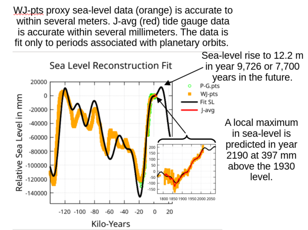
Here is shown the last 140,000 years of relative sea-level information, WJ-pts fit with a constant and 11 periodic functions associated with planetary orbital cycles (Fit SL, black, negative years are BCE dates). The peak at 12.2 meters is in the year 9,726 or 7,700 years into the future. Note that the peak at -119,600 is at 10.75 meters. The inset plot (see Figure 13 for details) shows how the fit matches with the Jevrejeva et al. [12] reconstructed sea-level data, 1807 to 2010 relative to 1930. The J-avg curve (red) is a 10-year running average over these years. The P-G-pts are proxy sea-level information from Physical Geology [6] and not input to the fit – see Appendix.
Figure 1.
Here is shown the last 140,000 years of relative sea-level information, WJ-pts fit with a constant and 11 periodic functions associated with planetary orbital cycles (Fit SL, black, negative years are BCE dates). The peak at 12.2 meters is in the year 9,726 or 7,700 years into the future. Note that the peak at -119,600 is at 10.75 meters. The inset plot (see Figure 13 for details) shows how the fit matches with the Jevrejeva et al. [12] reconstructed sea-level data, 1807 to 2010 relative to 1930. The J-avg curve (red) is a 10-year running average over these years. The P-G-pts are proxy sea-level information from Physical Geology [6] and not input to the fit – see Appendix.
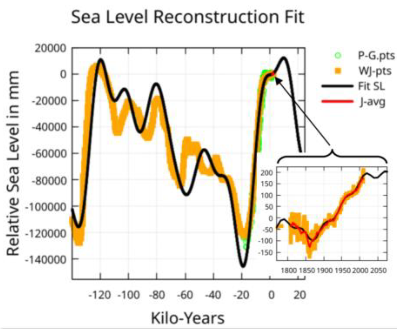
Figure 2.
Least squares fits were performed using a cubic and one period for a sequence of periods. The optimal period, reported here, provides the highest R squared value. Optimal periods were: 62.2 years for J-fit with R squared 0.955, 56.3 years for C-fit with R squared 0.986, and 58.5 years for D-fit with R squared 0.998.
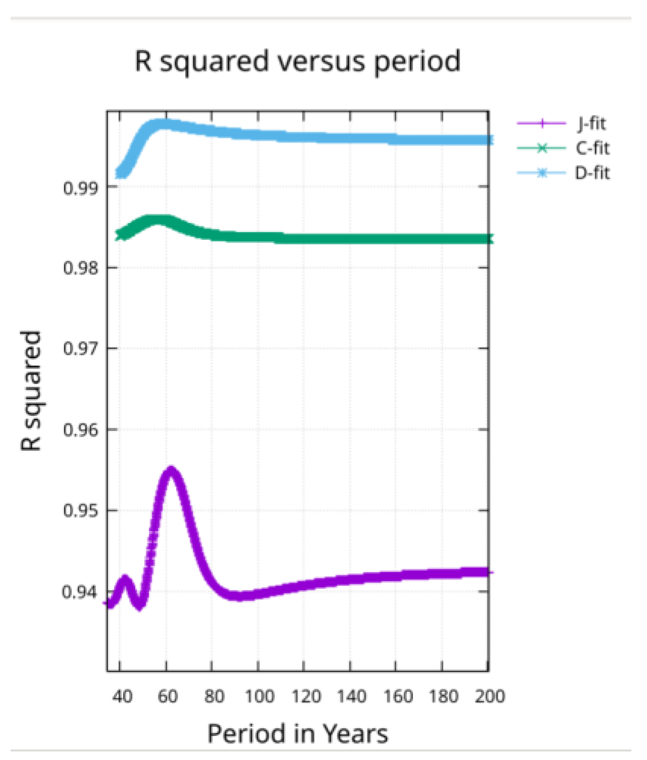
Figure 3.
Antarctic Ice Core proxy data for relative temperature, [12] . Interpolated to 10-year sampling and then averaged over 100 years.
Figure 3.
Antarctic Ice Core proxy data for relative temperature, [12] . Interpolated to 10-year sampling and then averaged over 100 years.
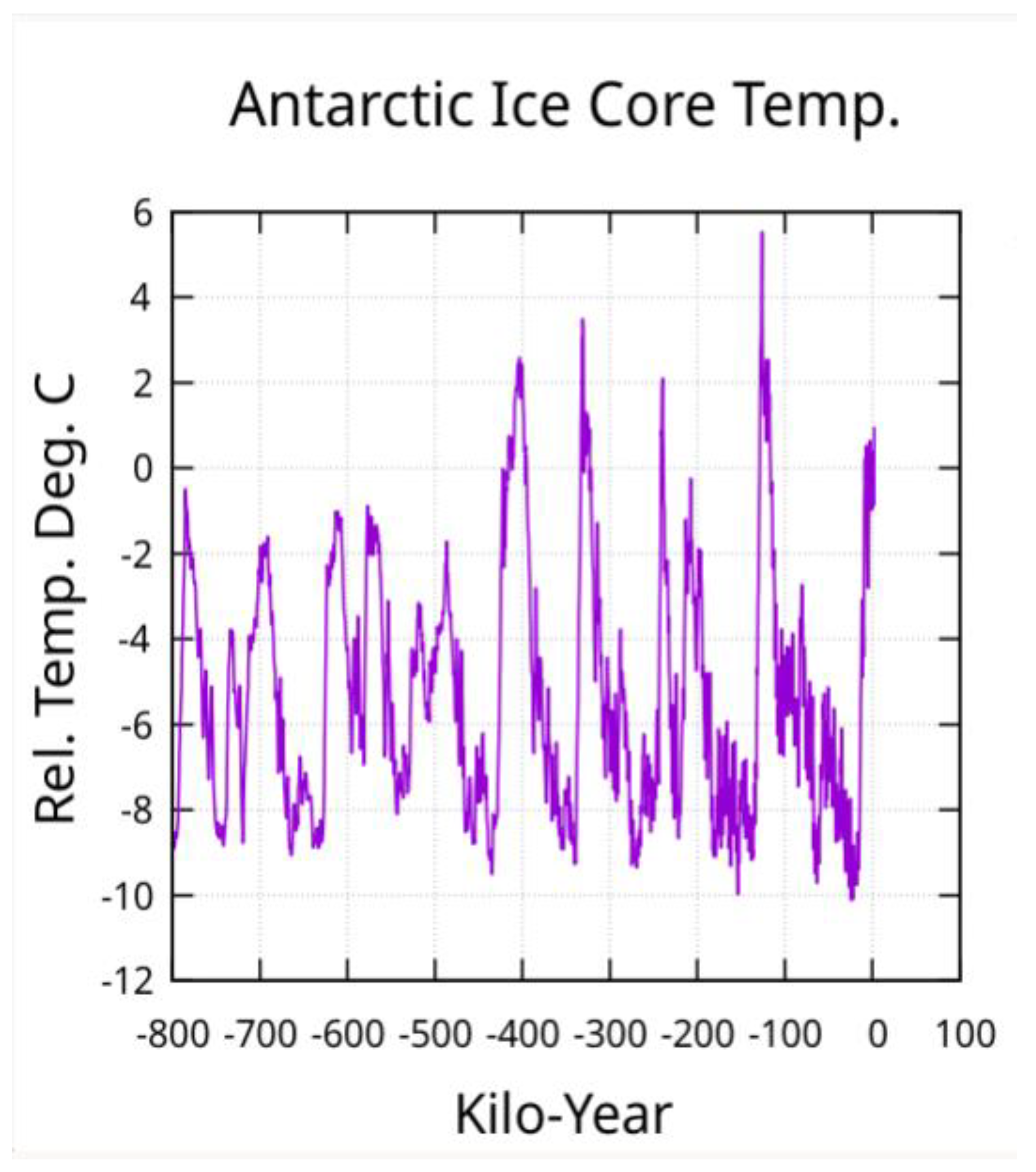
Figure 4.
Plot of sea-level reconstruction for Jevrejeva et al. (J-pts), Church and White (C-pts) and Dangendort et al. (D-pts) on top of the least squares fits to each. Separation is due to reconstructions being zeroed on different years.
Figure 4.
Plot of sea-level reconstruction for Jevrejeva et al. (J-pts), Church and White (C-pts) and Dangendort et al. (D-pts) on top of the least squares fits to each. Separation is due to reconstructions being zeroed on different years.
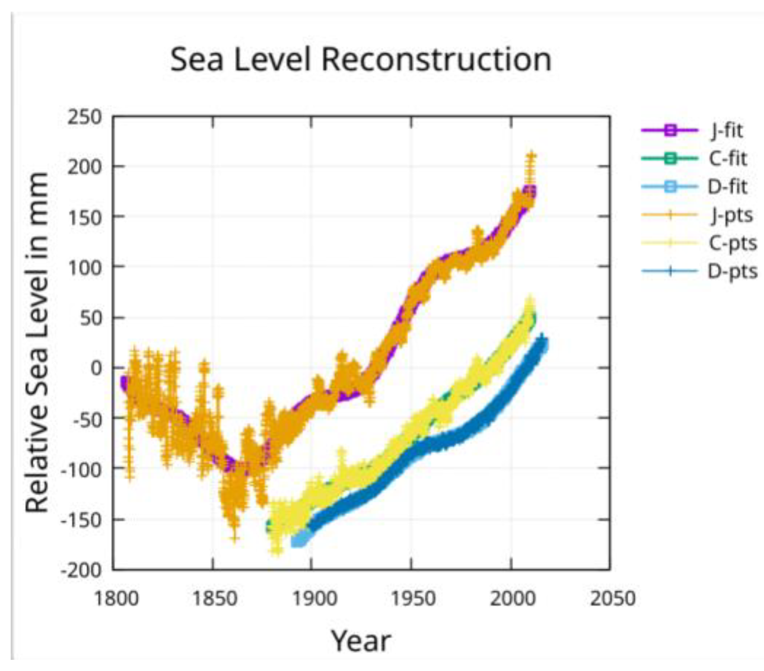
Figure 5.
First derivative (slope) of sea-level rise for the fits to the three reconstructions.
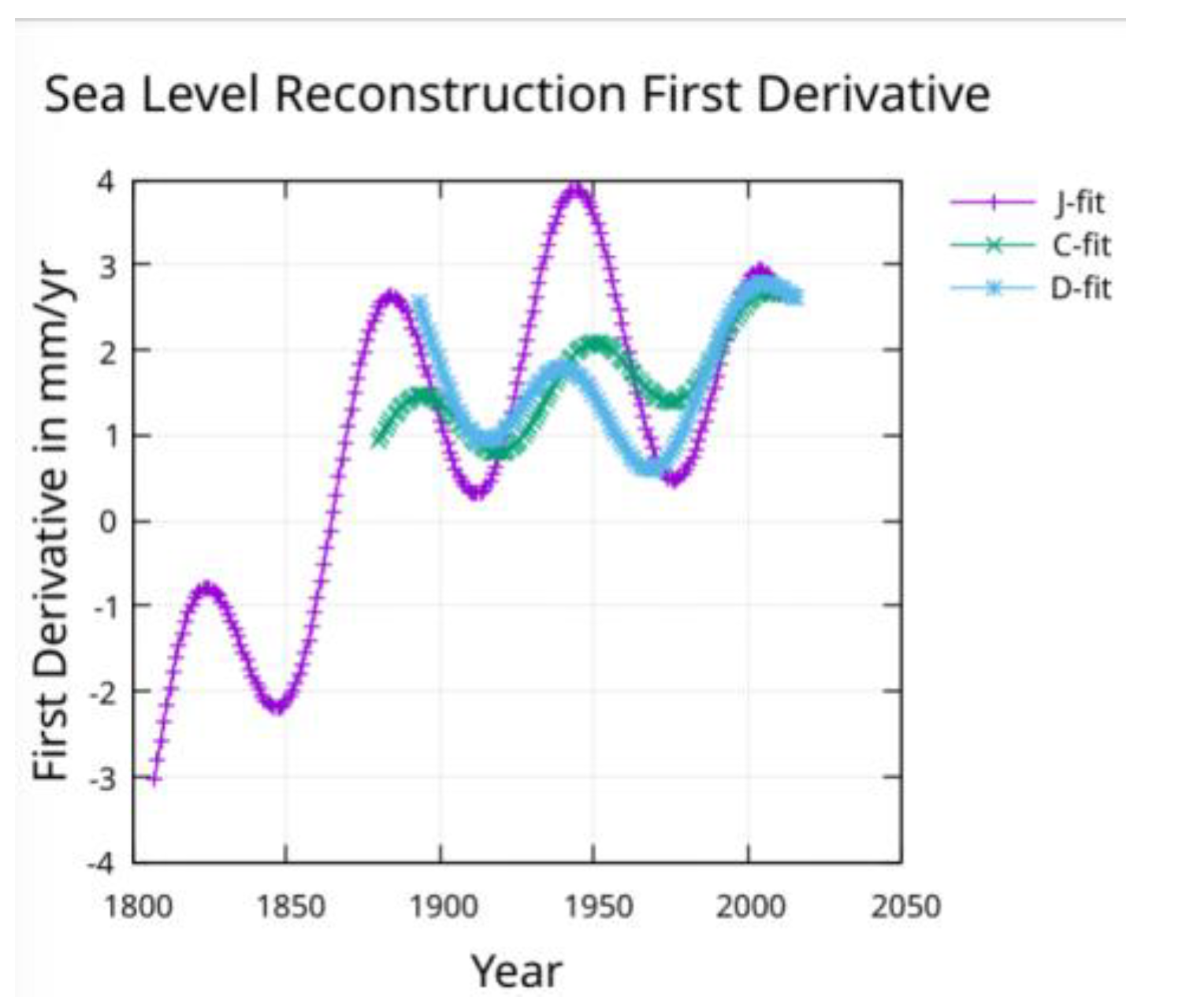
Figure 6.
Second derivative (acceleration) of the fits to the three reconstructions. The relative phase of the period for each reconstruction can be observed in the positions of the peaks in this plot.
Figure 6.
Second derivative (acceleration) of the fits to the three reconstructions. The relative phase of the period for each reconstruction can be observed in the positions of the peaks in this plot.
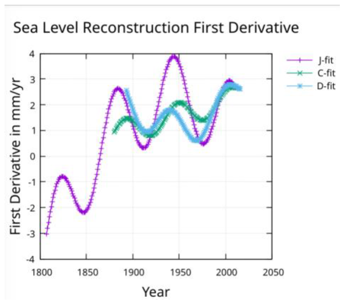
Figure 7.
The fits to the reconstructions are shown here with the 60-year period removed from the fit.
Figure 7.
The fits to the reconstructions are shown here with the 60-year period removed from the fit.
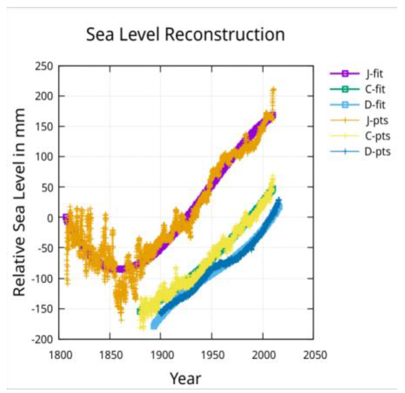
Figure 8.
The first derivative (slope) of the fit functions with the 60 year period removed.
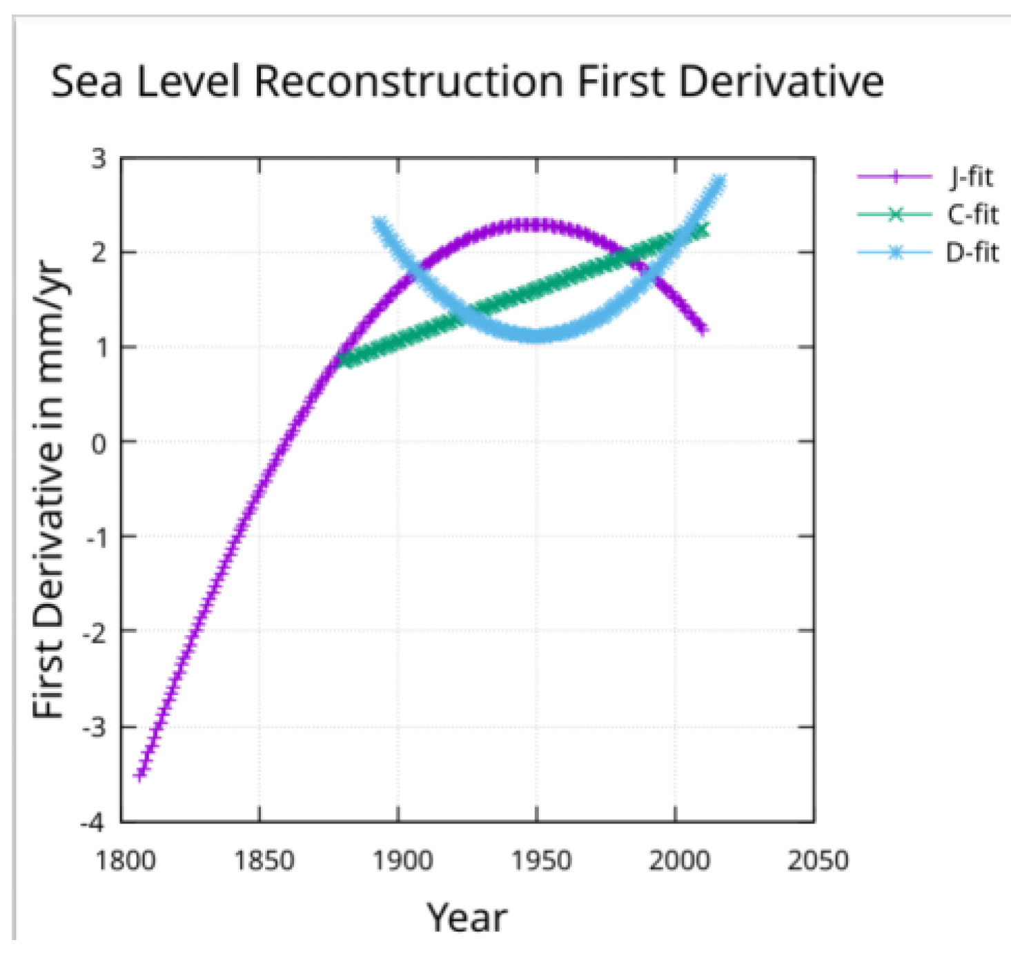
Figure 9.
The second derivative (acceleration) of the fits to the reconstructions with the 60-year period removed.
Figure 9.
The second derivative (acceleration) of the fits to the reconstructions with the 60-year period removed.
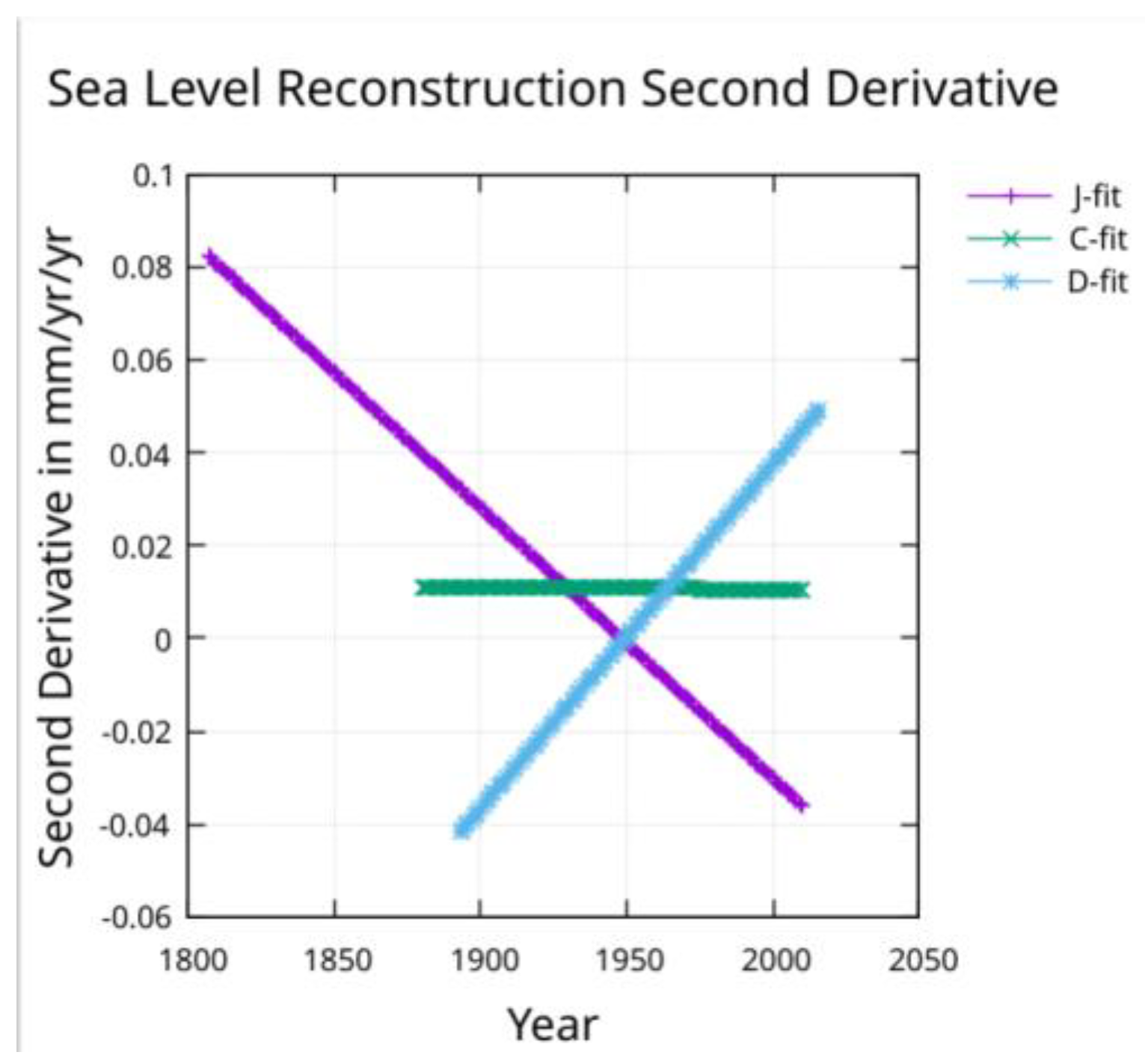
Figure 10.
The input data (orange squares, WJ-pts) represents 250,000 years of sea-level variation and includes the J-pts. Extrapolation a million years into the past and future (not shown) never exceed a sea-level rise of 40 meters above 1930’s relative level of zero – constraint (3). The P-G-pts are proxy sea-level points from Physical Geology and not input to the fit – see Appendix. The J-avg is a ten-year running average of the J-pts.
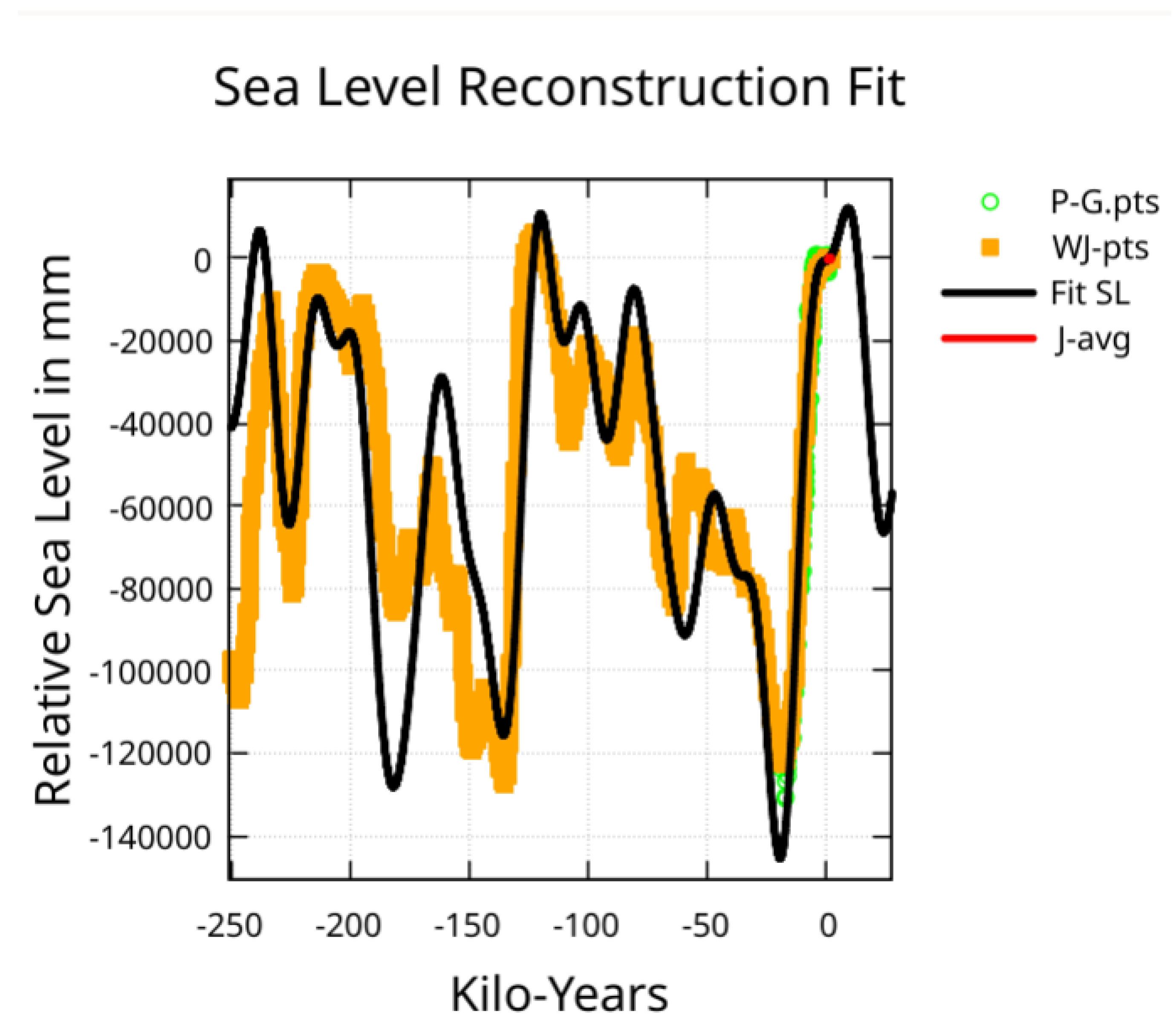
Figure 11.
Sea-level fit from -25ky to 5ky. The weight of the fit favors more recent time points strongly over old – see Appendix. Here the P-G data points (not input to the fit) are also plotted (PG-pts – see Appendix). The P-G data scatter indicates the level of uncertainty.
Figure 11.
Sea-level fit from -25ky to 5ky. The weight of the fit favors more recent time points strongly over old – see Appendix. Here the P-G data points (not input to the fit) are also plotted (PG-pts – see Appendix). The P-G data scatter indicates the level of uncertainty.
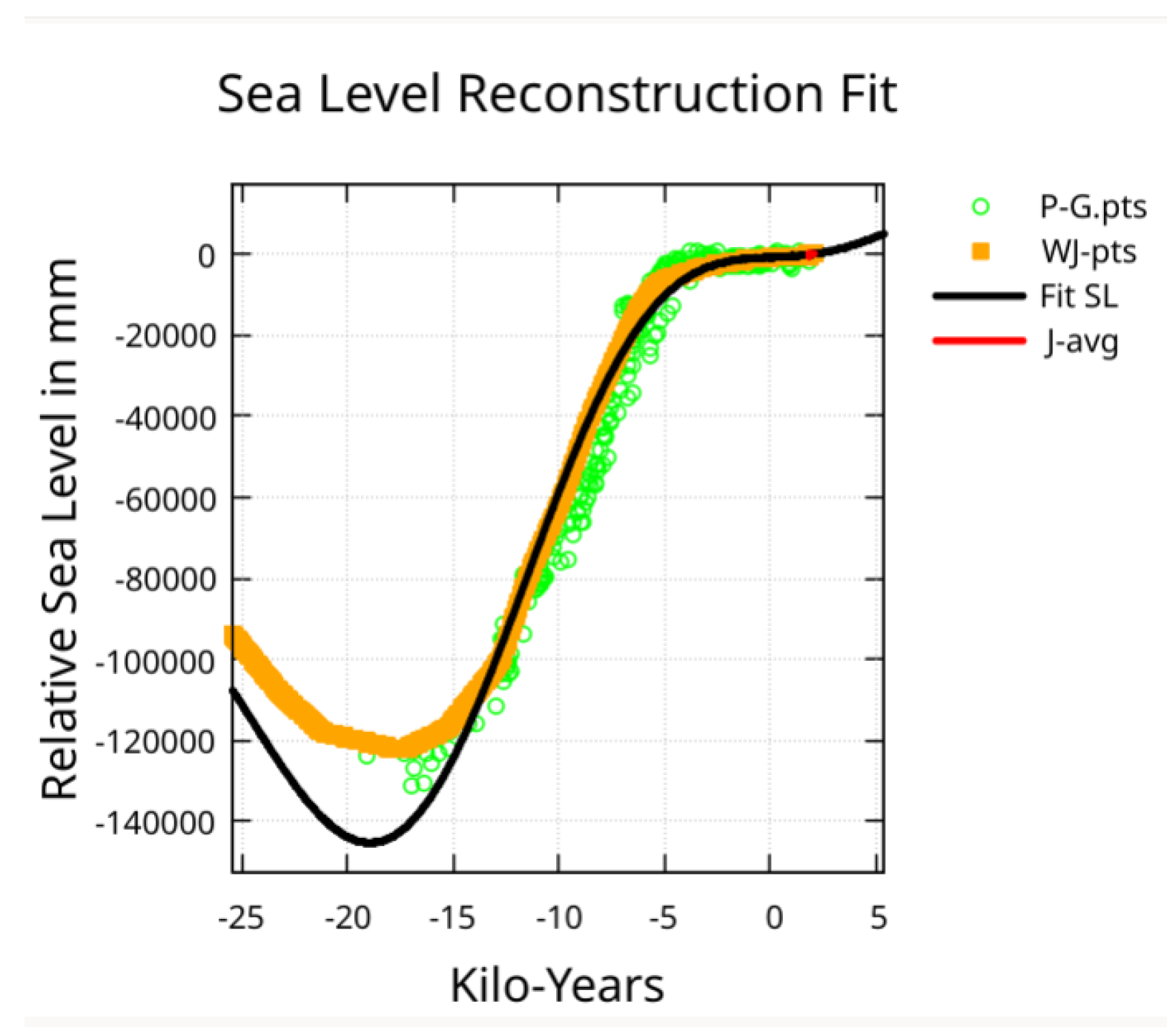
Figure 12.
Here is shown a zoom on the portion of the input data and fit that covers the time period prior to and after the Jevrejeva et al. sea-level reconstruction. Again, the PG-pts is plotted. The effect of the shorter period functions can be seen at this scaling.
Figure 12.
Here is shown a zoom on the portion of the input data and fit that covers the time period prior to and after the Jevrejeva et al. sea-level reconstruction. Again, the PG-pts is plotted. The effect of the shorter period functions can be seen at this scaling.
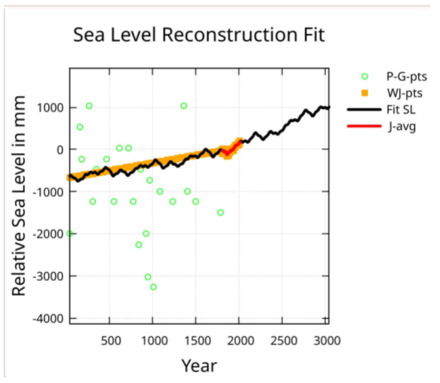

Table 1.
Summary of fit option characteristics.
| Options | Date of peak | Sea-level at date | Sea-level at -120 ky | R Sq. -120 ky |
R Sq. 20 ky |
R Sq. 1800 |
| A | 9,726 | 12 m | 11 m | 0.86 | 0.98 | 0.95 |
| B | 9,746 | 13 m | 11 m | 0.80 | 0.96 | … |
| C | 12,584 | 40 m | 8 m | 0.99 | 0.92 | 0.95 |
| D | 12,605 | 34 m | 12 m | 0.93 | 0.98 | 0.95 |
| E | 10,269 | 19 m | 9 m | 0.80 | 0.99 | 0.95 |
Table 2.
Periods used, and R squared for year 1800.
| R Sq. for year 1800 | Period | Period | Period | Period | Period |
| 0.362 | 58 yr | - | - | - | - |
| 0.490 | 58 yr | 89 yr | - | - | - |
| 0.598 | 58yr | 89 yr | 144 yr | - | - |
| 0.940 | 58 yr | 89 yr | 144 yr | 193 yr | - |
| 0.950 | 58 yr | 89 yr | 144 yr | 193 yr | 579 yr |
Disclaimer/Publisher’s Note: The statements, opinions and data contained in all publications are solely those of the individual author(s) and contributor(s) and not of MDPI and/or the editor(s). MDPI and/or the editor(s) disclaim responsibility for any injury to people or property resulting from any ideas, methods, instructions or products referred to in the content. |
© 2025 by the authors. Licensee MDPI, Basel, Switzerland. This article is an open access article distributed under the terms and conditions of the Creative Commons Attribution (CC BY) license (http://creativecommons.org/licenses/by/4.0/).
Copyright: This open access article is published under a Creative Commons CC BY 4.0 license, which permit the free download, distribution, and reuse, provided that the author and preprint are cited in any reuse.


