Submitted:
07 April 2025
Posted:
08 April 2025
You are already at the latest version
Abstract
In this study, a cantilever beam with a tip mass under base excitation was analyzed, with system damping modeled using a fractional derivative approach. By applying the Rayleigh-Ritz method, the governing equation was decomposed into spatial and temporal components. Analytical solutions for the temporal equation were derived; however, their complexity posed challenges for practical application. To address this, convergence acceleration techniques were employed to efficiently evaluate slowly converging series representations. Additionally, two methods for identifying the parameters of a classical model approximating the fractional system were investigated: a geometric approach based on waveform shape analysis and an optimization procedure utilizing a genetic algorithm.
Keywords:
fractional calculus
; fractional Kelvin-Voigt model
; piezoelectric energy harvester
; viscoelasticity
1. Introduction
A cantilever beam with piezoelectric layers and a tip mass under base excitation is a widely studied model in piezoelectric energy harvesting [1]. Damping in such beams has traditionally been modeled using classical derivative-based approaches [2]. Alternatively, fractional-order models have been employed to describe damping effects more accurately, capturing memory-dependent and nonlocal characteristics of viscoelastic materials [3,4,5].
The Galerkin and Rayleigh-Ritz methods are commonly employed to solve problems involving vibrating beams and other mechanical structures such as rods and plates [3,6]. These methods enable the decomposition of the solution of the governing equation into two components: spatial and temporal. Typically, the temporal solution is predetermined, as it often corresponds to the natural vibration modes of the mechanical structure under consideration or is represented by appropriately chosen, well-established functions.
In this study, the vibration of a beam with a tip mass under base excitation is analyzed. The damping in the system is modeled using a fractional Kelvin-Voigt constitutive equation for a viscoelastic material [7]. The application of the Rayleigh-Ritz method reduces the problem to a set of independent fractional differential equations, each corresponding to a distinct natural vibration mode of the beam. These equations take the following form:
where represents the temporal component of the solution associated with a specific natural vibration mode, and are fixed real parameters, is the order of the fractional derivative , and represents the excitation term corresponding to the given vibration mode.
In the literature, the model described by equation (1) is referred to as the fractional Kelvin-Voigt (FKV) oscillator [8]. It attracted the attention of many researchers [9,10,11,12,13]. Some studies employ the Riemann-Liouville definition of the fractional derivative [9], while others use the Caputo definition [12]. Although analytical solutions to Eq. (1) have been derived [11,14,15], numerical methods are often preferred for solving this equation due to the complexity of the analytical solutions and the computational challenges associated with their practical application. In contrast, classical models with integer-order derivatives do not exhibit such difficulties.
This naturally raises the question: under what conditions can fractional models be replaced by classical models, and how should the parameters of classical models be selected to best approximate the behavior of fractional models? A similar problem has been investigated in [16,17,18,19] using different approaches. The Fourier transform and the response of oscillators to a unit impulse were analyzed in [16]. In [17] the total mechanical energy of fractional operators was used to determine the damping coefficient of a classical model corresponding to a fractional model. The relationship between fractional and classical models was established in [18] by matching their dispersion relations. Finally, in [19] a measure of the incompatibility between fractional and classical models, referred to as the divergence coefficient, was introduced, and optimization methods were employed to refine the parameter selection.
This article presents a method for determining the solution of Eq. (1) using closed-form analytical formulas, complemented by a numerical approach to accelerate the convergence of slowly converging series, specifically the Wynn-epsilon method [20]. Typically, equations of this type are solved using purely numerical techniques [21,22] due to the complexity of their analytical solutions. However, obtaining solutions in a closed form is of significant importance, as they provide a benchmark for validating numerical methods and assessing their accuracy.
To determine the classical model—a damped harmonic oscillator, corresponding to a given FKV oscillator—two approaches are employed. In the first approach, the parameters of the classical model—namely, the undamped angular frequency and the damping ratio—are identified by analyzing the shape of the response graph. This includes examining the distribution of zeros and the positions of local maxima, with the logarithmic decrement method applied to the latter [23]. The second approach utilizes the divergence coefficient introduced in [19]. The parameters of the classical model are estimated by minimizing the divergence coefficient using a genetic algorithm. The results obtained from both approaches are compared and discussed.
The paper is structured as follows. The introduction outlines the current state of research and presents the scope of the study in relation to previous work. In the next section, the fractional Kelvin–Voigt (FKV) oscillator equation is obtained as the temporal part of the motion of a cantilever beam with a tip mass subjected to base excitation. The following section presents analytical solutions to both the homogeneous and nonhomogeneous forms of the FKV equation for Riemann–Liouville and Caputo derivatives, and discusses two methods for identifying the parameters of an equivalent harmonic oscillator. The results section includes validation of the numerical method based on analytical formulas, evaluation of the identified harmonic models, and their performance in the nonhomogeneous case. The final section presents the conclusions of the study.
2. Formulation, Solution, and Computational Methods
2.1. Governing Equation and Solution Using the Rayleigh-Ritz Method
Consider a cantilever beam, clamped at , with a tip mass at its free end , subjected to base excitation, as shown in Figure 1. Assume that the relationship between stress and strain in the beam’s material is governed by a constitutive equation known as the fractional Kelvin-Voigt model [7]:
where is a material constant, is retardation time, and is the order of the fractional derivative , with , which is taken with respect to only.
According to Euler-Bernoulli’s beam bending theory, the relationship between strain and the transverse displacement of the beam is given by:
The bnding moment in the beam cross section is determined as:
By substituting Eqs. (2)-(4) into the equilibrium equation:
one obtains the governing equation for the transverse displacement :
where is the moment of inertia of the cross-section with respect to the bending axis , is the cross-sectional area, is a density of beam’s material. The absolute transverse displacement can be expressed as:
where is the displacement relative to a moving coordinate system with its origin at the clamped end of the beam, and is the base displacement. It is assumed that:
where and are amplitude and angular frequency of the base excitation respectivelly. Substituting Eqs. (7) and (8) into Eq. (6) yields:
The boundary conditions for displacement and angle at clamped end are:
The boundary condition for the bending moment at the free end is:
The boundary condition for the transverse force at the free end is the following:
where is the mass of the body attached to the free end of the beam and is its moment of inertia about (for point mass it would be equal to ).
To obtain an approximate solution to Eq. (9), the Rayleigh-Ritz method is employed. In this approach, the transverse displacement is assumed to be a series expansion in terms of trial functions that satisfy the boundary conditions:
where are the trial functions representing the mode shapes of the beam, and are the generalized coordinates that describe the time-dependent motion of the system. The mode shapes of a cantilever beam are given by [1,24]:
where:
and dimensionless eigenvalues are determined from the characteristic equation:
Eigenfunctions defined in Eq. (14) are orthogonal, which means that for , the following conditions hold:
for , these integrals are nonzero.
Multiplying Eq. (9) by and integrating over the range , we obtain, based on the orthogonality conditions of the natural vibration modes (17), an equation of the form (1), as previously introduced, where the function is defined as:
For some associated with the -th vibration mode of the beam.
2.2. Solution of the Temporal Equation and Numerical Methods
In this section, we present closed-form solutions for Eq. (1) and discuss numerical methods for their efficient computation.
We begin with the homogeneous equation for :
We consider the above equation with initial conditions: , .
Based on Theorem 5.2 and Proposition 5.2 from [14], and after applying the necessary transformations, the solution of Eq. (19) for the Riemann–Liouville fractional derivative takes the form::
where:
Similarly, applying Theorem 5.13 and Proposition 5.8 from [14], the solution for Eq. (19) in the case of the Caputo fractional derivative takes the form:
where:
For the nonhomogeneous Eq. (1), solutions can be obtained for both Riemann-Liouville and Caputo fractional derivatives using Proposition 5.5 and Proposition 5.11, respectively, in the form:
where the function is defined as:
The function represents the solution of the homogeneous Eq. (19) for either the Riemann-Liouville or Caputo derivative, as given in Eqs. (20) and (23), respectively.
Direct computation of and by truncating the series in Eqs. (21), (22), (24), and (26) is only effective for small values of t. For larger , naive truncation leads to significant numerical errors due to cancellation and round-off in the summation of highly oscillatory terms. To overcome this limitation and extend the computation to a broader range of , we employed the Wynn- algorithm [20], as implemented in Mathematica’s built-in function SequenceLimit[]. The integral in Eq. (25) was evaluated using the trapezoidal rule. Our calculations were performed using Mathematica v. 12.1.
Applying the Wynn- method requires transforming the double series into a single series. Since the original series are absolutely convergent, their terms can be grouped and summed in an arbitrary order. Here, summation was performed over , varying from zero to infinity. The computations required high floating-point precision, and all model parameters were converted into symbolic fractions to facilitate exact symbolic calculations. While this approach eliminated rounding errors, it significantly increased computation time.
The computational domain was chosen to approximately span ten fundamental periods of the homogeneous solution . To determine , the fundamental frequency of the corresponding harmonic oscillator was estimated using the relation derived in [19]:
The final time was then set as , with .
The time step for evaluating the integral in Eq. (25) using the trapezoidal rule was chosen as .
2.3. Identification of Equivalent Harmonic Oscillator Parameters: Geometric and Optimization Approaches
The classical damped harmonic oscillator is well known to be governed by equation:
subject to the initial conditions , . Here, denotes the undamped natural angular frequency of the system, and is the damping ratio. The solution to Eq. (28) can be written in the form:
where the functions and are expressed in terms of exponential and trigonometric functions.
Our aim is to determine an equivalent harmonic oscillator represented by Eq. (28) that approximates the behavior of the FKV oscillator, defined by Eq. (19). Solutions of the Eq. (19) for the case of the Riemann-Liouville and Caputo fractional derivatives, given by formulas (20) and (23) respectively, share a common component corresponding to the initial condition . Consequently, if a harmonic oscillator can be identified for the case of the Caputo fractional derivative, it remains the same for the case of Riemann-Liouville fractional derivative. In this work, we choose to focus primarily on the Caputo fractional derivative. This is motivated by the fact that, unlike the Riemann–Liouville derivative, the Caputo formulation allows for the use of physically meaningful initial conditions expressed in terms of the function and its integer-order derivatives, such as position and velocity.
2.3.1. Geometric Approach to Parameter Identification
As a result of the numerical method of solving equation (19), we have the values of the components and defined in Eqs. (24) and (22), respectively, at discrete moments of time , for some , . Here we discuss how, based on these data, to obtain approximations of the parameters and of a harmonic oscillator that approximates a given FKV oscillator.
Let the sequences and represent, respectively, the approximate locations of the zeros and the arguments corresponding to local maxima of the function . Similarly, the sequences and are defined for the function . The approximate parameters of the harmonic oscillator corresponding to the given FKV oscillator are determined from the following formulas:
In the denominator of equation (30), we approximate half the fundamental period for the harmonic oscillator we are looking for, so dividing by half the period give an approximation of the circular frequency . In equation (31), we use the concept of logarithmic damping decrement to determine .
2.3.2. Genetic Algorithm Approach to Parameter Identification
To assess the quality of fit between a given FKV oscillator and a classical harmonic oscillator, we adopted a measure of model similarity defined in [19] called the divergence coefficient:
where is supremum norm on intervalfor some [25], and are defined in (23) and (28) respectively. Divergence coefficient has an interpretation as the maximum relative difference between components of the functions and . Function is fixed and we look for the function that minimizes the divergence coefficient (32). In this case we write .
Let the FKV oscillator with parameters be fixed. We use the genetic algorithm to find the minimum value of the divergence coefficient and the parameters and of harmonic oscillator, which correspond to the given FKV oscillator. The calculations were carried out using MATLAB's ‘Global Optimisation’ toolbox. The objective function, the divergence coefficient, was minimized using MATLAB's built-in function ga. Although the ga function allows adjusting many parameters, after experimenting with various settings, we decided to use its default options. Changes in the parameters typically did not significantly improve the result's quality, but often substantially increased computation time.
3. Results
3.1. Verification of the Wynn-Epsilon Method for Solving the FKV Oscillator Equation
To validate the numerical method used to evaluate the series solutions of Eq. (19), we consider the special case . In this case, Eq. (19) reduces to the classical damped harmonic oscillator equation (28), with parameters given by and . Accordingly, we substitute into Eqs. (21), (22), and (24), and compare the results obtained using the Wynn-epsilon method with the known analytical functions and appearing in Eq. (29). This comparison allows us to verify the correctness and numerical accuracy of the proposed approach.
Figure 2, Figure 3 and Figure 4 present a comparison between the analytical solution components of the classical harmonic oscillator, and (solid black lines), and the corresponding approximations obtained using the Wynn-epsilon method for the fractional model with Riemann–Liouville (red dashed lines) and Caputo (blue dashed lines) derivatives.
Subfigures labeled (a) show the components associated with the initial displacement condition , while subfigures labeled (b) correspond to the initial velocity condition . It should be noted that in the subfigures (b), only two curves are plotted, since the solution components related to the initial velocity are identical for both the Riemann–Liouville and Caputo cases.
A very good agreement can be observed between the Wynn- approximation of the and the function in Figure 2, Figure 3 and Figure 4(a), with the maximum relative absolute difference being on the order of . A similar observation holds for the Wynn- approximation and the function shown in Figure 2, Figure 3 and Figure 4(b).
In contrast, noticeable discrepancies occur between (red dashed lines in Figure 2, Figure 3 and Figure 4(a)) and , with maximum relative differences reaching approximately 0.36 in Figure 2(a), 0.55 in Figure 3(a), and 0.09 in Figure 4(a). These deviations are related to the incompatibility of initial conditions in the Riemann–Liouville formulation. However, it can be shown that the difference tends to zero as , indicating that the solutions converge asymptotically.
To validate the numerical solutions of the nonhomogeneous fractional Kelvin–Voigt oscillator equation with zero initial conditions, we once again consider the limiting case . In this case, the equation reduces to the classical nonhomogeneous damped harmonic oscillator:
where , , and the forcing function is defined in Eq. (18). We denote the solution of Eq. (33) under zero initial conditions by . This solution serves as a reference for assessing the accuracy of the numerical results obtained for the fractional model with .
Let denote the solution of Eq. (1) with zero initial conditions for . In this case, the homogeneous component vanishes, and the solution is given by the convolution integral appearing in Eq. (25).
To illustrate the accuracy of the proposed numerical approach, Figure 5 presents a comparison between the exact solution of the classical oscillator equation (33) and the approximation obtained using the Wynn-epsilon method. The comparison is carried out for two selected fractional Kelvin–Voigt oscillators subjected to the external excitation defined in Eq. (18), with parameters fixed as and .
The agreement between the exact solution and the Wynn-epsilon approximation is very good. The maximum relative difference between the two curves is on the order of .
3.2. Identification of Equivalent Harmonic Oscillator Parameters: Geometric and Optimization Approaches
In this section, we compare two methods for identifying the parameters of a classical harmonic oscillator that best approximates the response of a given fractional Kelvin–Voigt (FKV) oscillator. For each method, denoted by the superscript , we define the identified optimal parameters of the equivalent harmonic oscillator as and , corresponding to the undamped natural frequency and the damping ratio, respectively.
The resulting optimal approximation is denoted by , and its accuracy is evaluated using formula , where denotes the divergence coefficient defined in Eq. (32), which quantifies the discrepancy between the fractional and harmonic oscillator responses.
Table 1 presents a comparison of parameter identification results for several fractional Kelvin–Voigt (FKV) with parameters shown in the first column. For each case, the identified parameters of the equivalent harmonic oscillator obtained using the geometric method (second column) and the genetic algorithm (third column) are listed, along with the corresponding values of the divergence coefficient , which quantifies the discrepancy between the fractional and classical models.
Analysis of the results reveals that the genetic algorithm generally yields lower values of the divergence coefficient , indicating better agreement between the models. However, this is not always the case, as illustrated by rows 1 and 7 of Table 1, where the geometric method performs slightly better. In certain cases (rows 7 and 10), the divergence coefficient reaches relatively high values, suggesting that the classical harmonic model may not always provide a satisfactory approximation of the fractional dynamics.
Figure 6, Figure 7, Figure 8 and Figure 9 6–9 present a comparison between the solution components of selected FKV oscillators and those of classical harmonic oscillators identified using two different methods: a geometric approach and a genetic algorithm. Each figure is composed of two parts (a) and (b). Figures (a) show comparison of the displacement-related components and , while figures (b) comparison of the velocity-related components and . Here, and correspond to components of the harmonic oscillator solution computed using the optimal parameters obtained via the respective identification method.
The results illustrated in Figure 6, Figure 7, Figure 8 and Figure 9 provide additional insight into the effectiveness of both identification methods in approximating the behavior of various FKV oscillators. The observations are consistent with the divergence values reported in Table 1.
In Figure 6, corresponding to parameters , both methods yield harmonic oscillators with relatively high divergence values (around 0.08), despite the overall good visual agreement of the solution components. Deviations are mainly noticeable near the extrema of the curves, as seen in part (a) of the figure.
Figure 7 shows results for , where the divergence coefficients are somewhat different—0.037 for the geometric method and 0.026 for the genetic algorithm—yet in both cases the visual agreement between the fractional and classical components is excellent.
In Figure 8, with parameters , a more pronounced discrepancy is observed: the geometric approach produces a relatively large value of the , while the genetic algorithm yields a smaller value. This case corresponds to a system with strong damping, which may contribute to the increased difficulty in achieving an accurate harmonic approximation.
Finally, Figure 9, representing , shows that neither method succeeds in producing a good match. The divergence coefficient exceeds 0.1 in both cases, reaching as high as 0.25 for the geometric approach. This poor agreement, clearly visible in both components, suggests that for this configuration, a classical harmonic oscillator may not adequately capture the dynamics of the fractional system.
3.3. Testing Harmonic Models in the Nonhomogeneous Case
In this subsection, we investigate the performance of the identified harmonic oscillator models in the context of the nonhomogeneous fractional Kelvin–Voigt equation (Eq. (1)) with zero initial conditions. The solution of this equation, given by Eq. (25), reduces to a convolution integral, as the homogeneous part vanishes. For comparison, we consider the classical damped harmonic oscillator (Eq. (33)) with zero initial conditions and identical sinusoidal forcing, whose solution can be expressed in closed form using elementary functions such as sine, cosine, and exponential terms.
The harmonic oscillator parameters used in this comparison were obtained using the identification methods described in the previous subsection, for fixed values of the FKV model parameters . Two representative FKV oscillators were selected for this analysis: and . The corresponding harmonic oscillator parameters are listed in Table 1 (rows 1 and 5, respectively).
To quantitatively assess the agreement between the solutions of the fractional model and the classical harmonic oscillator , we use a modified version of the divergence coefficient (32) introduced earlier:
Specifically, when the indicator defined in Eq. (34) is evaluated using the solution obtained with parameters identified in the previous subsection (using either the geometric method or the genetic algorithm), we denote its value by .
Figure 10 and Figure 11 present a comparison between the time-domain responses of the fractional oscillator and the corresponding harmonic oscillator approximations , obtained using the geometric method (red dashed lines) and the genetic algorithm (blue dashed lines). The fractional response is plotted in black as a reference.
For each selected FKV oscillator, two scenarios are considered: one in which the forcing frequency is far from the resonance frequency of the harmonic model, and another in which is chosen to match the resonance frequency of the harmonic model (we set ). This setup allows us to examine how the accuracy of the harmonic approximation depends on the proximity to resonance.
The results shown in Figure 10 and Figure 11 highlight the influence of the forcing frequency on the accuracy of harmonic oscillator approximations in the nonhomogeneous case. Each figure compares the solution of the FKV equation with those of two harmonic oscillators identified using the geometric method and the genetic algorithm, respectively.
For the FKV oscillator with parameters , subfigure 10(a) illustrates the resonance case with , where substantial discrepancies are observed: the divergence coefficients reach for the geometric method and for the genetic algorithm. In contrast, subfigure 10(b), corresponding to the off-resonance case with , shows very good agreement, with dropping to and , respectively.
A similar trend is visible for the oscillator defined by . In this case, the off-resonance response (subfigure 11(a)), yields relatively low divergence values: for the geometric method and for the genetic algorithm. However, the resonance case shown in subfigure 11(b), with , leads to a complete breakdown of the harmonic approximation, with divergence values near to 1 for both methods.
These results demonstrate that while harmonic oscillator models can accurately reproduce the fractional response under off-resonance excitation, they may fail dramatically near resonance. This is due to the high sensitivity of the system’s steady-state behavior in the resonant regime, where subtle differences in the underlying dynamics—especially those introduced by the fractional-order operator—are strongly amplified and no longer well captured by classical models.
To further investigate the sensitivity of the harmonic approximation with respect to the forcing frequency, we compute the divergence coefficient for a range of excitation frequencies. Specifically, we vary the ratio from to in steps of , while keeping the parameters of the FKV oscillator fixed. This analysis is performed for both identification methods and for the two representative FKV oscillators considered earlier.
The plots in Figure 12 reveal that the divergence coefficient reaches a sharp peak in the vicinity of , confirming that the accuracy of the harmonic approximation deteriorates significantly near resonance.
For the first FKV oscillator (Figure 12(a)), the peak is less pronounced and slightly shifted away from . This shift reflects the fact that the actual resonance frequency of the corresponding harmonic oscillator does not exactly match the parameter of the FKV model.
In contrast, for the second oscillator (Figure 12(b)), the resonance frequency of the harmonic model is close to , resulting in a stronger and more centered peak. These observations highlight the limitations of harmonic approximations in capturing resonant behavior in fractional-order systems.
4. Conclusions
This paper considered the dynamic response of a cantilever beam with a tip mass subjected to base excitation. The beam material was assumed to obey a fractional Kelvin–Voigt constitutive law. By applying modal decomposition, a time-domain equation governing the selected mode shape was derived. It was shown that the resulting model corresponds to the FKV oscillator equation.
A method for computing accurate time-domain solutions based on analytical series expressions was presented. The series, evaluated using the Wynn-epsilon algorithm, provide high accuracy at the cost of significant computational effort. While purely numerical methods may be more efficient in practical applications, the ability to compute highly accurate reference solutions based on analytical formulas is of great importance, as it enables reliable validation and benchmarking of approximate numerical schemes. The method was validated against exact solutions for the case . It was also observed that, for the Riemann–Liouville derivative, the component associated with the initial displacement condition deviates from the exact solution. This discrepancy is not due to numerical inaccuracy but rather reflects the known issues related to initial conditions for this type of derivative.
For a given FKV oscillator, two methods were proposed for identifying the parameters of an equivalent classical harmonic oscillator: a geometric approach and a genetic algorithm. Both methods yielded comparable accuracy in most cases, although the genetic algorithm generally produced better results.
Finally, the identified harmonic oscillators were applied to the nonhomogeneous version of the problem with sinusoidal forcing. The harmonic approximation was shown to be accurate when the forcing frequency was far from resonance, but its performance degraded significantly near the resonance frequency of the harmonic model.
Author Contributions
Conceptualization, P.Ł.; methodology, P.Ł.; software, P.Ł.; validation, P.Ł.; formal analysis, P.Ł.; investigation, P.Ł.; resources, P.Ł. data curation, P.Ł.; writing—original draft preparation, P.Ł.; writing—review and editing, P.Ł.; visualization, P.Ł.; supervision, P.Ł.; All authors have read and agreed to the published version of the manuscript.
Funding
This research received no external funding.
Data Availability Statement
The data presented in this study are available in this article.
Conflicts of Interest
The authors declare no conflicts of interest.
Abbreviations
The following abbreviations are used in this manuscript:
| FKV | Fractional Kelvin-Voigt |
| HO | Harmonic oscillator |
References
- Erturk, A.; Inman, D.J. Piezoelectric Energy Harvesting; 2011; ISBN 9780470682548.
- Basson, M.; De Villiers, M.; Van Rensburg, N.F.J. Solvability of a Model for the Vibration of a Beam with a Damping Tip Body. J. Appl. Math. 2014, 2014. [Google Scholar] [CrossRef]
- Paunović, S.; Cajić, M.; Karličić, D.; Mijalković, M. A Novel Approach for Vibration Analysis of Fractional Viscoelastic Beams with Attached Masses and Base Excitation. J. Sound Vib. 2019, 463. [Google Scholar] [CrossRef]
- Freundlich, J. Transient Vibrations of a Fractional Kelvin-Voigt Viscoelastic Cantilever Beam with a Tip Mass and Subjected to a Base Excitation. J. Sound Vib. 2019, 438, 99–115. [Google Scholar] [CrossRef]
- Freundlich, J. Transient Vibrations of a Fractional Zener Viscoelastic Cantilever Beam with a Tip Mass. Meccanica 2021, 56, 1971–1988. [Google Scholar] [CrossRef]
- Fasana, A.; Marchesiello, S. Rayleigh-Ritz Analysis of Sandwich Beams. J. Sound Vib. 2001, 241, 643–652. [Google Scholar] [CrossRef]
- Mainardi, F. Fractional Calculus and Waves in Linear Viscoelasticity: An Introduction to Mathematical Models; World Scientific, 2010; ISBN 9781848163300.
- Rossikhin, Y.A.; Shitikova, M. V. Application of Fractional Calculus for Dynamic Problems of Solid Mechanics: Novel Trends and Recent Results. Appl. Mech. Rev. 2010, 63, 1–52. [Google Scholar] [CrossRef]
- Zhang, W.; Shimizu, N. Damping Properties of the Viscoelastic Material Described by Fractional Kelvin-Voigt Model. JSME Int. Journal, Ser. C Dyn. Control. Robot. Des. Manuf. 1999, 42, 1–9. [Google Scholar] [CrossRef]
- Rossikhin, Y.A.; Shitikova, M. V. Application of Fractional Derivatives to the Analysis of Damped Vibrations of Viscoelastic Single Mass Systems. Acta Mech. 1997, 120, 109–125. [Google Scholar] [CrossRef]
- Vaz, J.; de Oliveira, E.C. On the Fractional Kelvin-Voigt Oscillator. Math. Eng. 2022, 4, 1–23. [Google Scholar] [CrossRef]
- Cao, Q.; Hu, S.L.J.; Li, H. Frequency/Laplace Domain Methods for Computing Transient Responses of Fractional Oscillators. Nonlinear Dyn. 2022, 108, 1509–1523. [Google Scholar] [CrossRef]
- Kim, V.A.; Parovik, R.I. Application of the Explicit Euler Method for Numerical Analysis of a Nonlinear Fractional Oscillation Equation. Fractal Fract. 2022, 6, 1–19. [Google Scholar] [CrossRef]
- Kilbas, A.; Srivastava, H.; Trujillo, J. Theory and Applications of Fractional Differential Equations; 2006; Vol. 129; ISBN 978-0-444-51832-3.
- Podlubny, I. Fractional Differential Equations, Volume 198: An Introduction to Fractional Derivatives, Fractional Differential Equations, to Methods of Their; Elsevier, 1998; Vol. 198; ISBN 978-0125588409.
- Li, M. Three Classes of Fractional Oscillators. Symmetry (Basel). 2018, 10. [Google Scholar] [CrossRef]
- Yuan, J.; Zhang, Y.; Liu, J.; Shi, B.; Gai, M.; Yang, S. Mechanical Energy and Equivalent Differential Equations of Motion for Single-Degree-of-Freedom Fractional Oscillators. J. Sound Vib. 2017, 397, 192–203. [Google Scholar] [CrossRef]
- Ding, W.; Hollkamp, J.P.; Patnaik, S.; Semperlotti, F. On the Fractional Homogenization of One-Dimensional Elastic Metamaterials with Viscoelastic Foundation. Arch. Appl. Mech. 2022. [Google Scholar] [CrossRef]
- Łabędzki, P.; Pawlikowski, R. On the Equivalence between Fractional and Classical Oscillators. Commun. Nonlinear Sci. Numer. Simul. 2023, 116, 106871. [Google Scholar] [CrossRef]
- Wynn, P. On a Device for Computing the em(Sn) Transformation. Math. Tables Other Aids to Comput. 1956, 10, 91–96. [Google Scholar] [CrossRef]
- Li, C.; Zeng, F. Numerical Methods for Fractional Calculus; 2015; ISBN 9781482253818.
- Garrappa, R. Numerical Solution of Fractional Differential Equations: A Survey and a Software Tutorial. Mathematics 2018, 6. [Google Scholar] [CrossRef]
- Little, J.A.; Mann, B.P. Optimizing Logarithmic Decrement Damping Estimation through Uncertainty Propagation. J. Sound Vib. 2019, 457, 368–376. [Google Scholar] [CrossRef]
- Weaver Jr, W.; Timoshenko, S.P.; Young, D.H. Vibration Problems in Engineering; John Wiley \& Sons, 1991.
- Rudin, W. Principles of Mathematical Analysis; 3rd ed.; McGraw-Hill: New York, 1976; ISBN 9780070542358.
Figure 1.
Model of a cantilever beam with a tip mass subjected to base excitation.
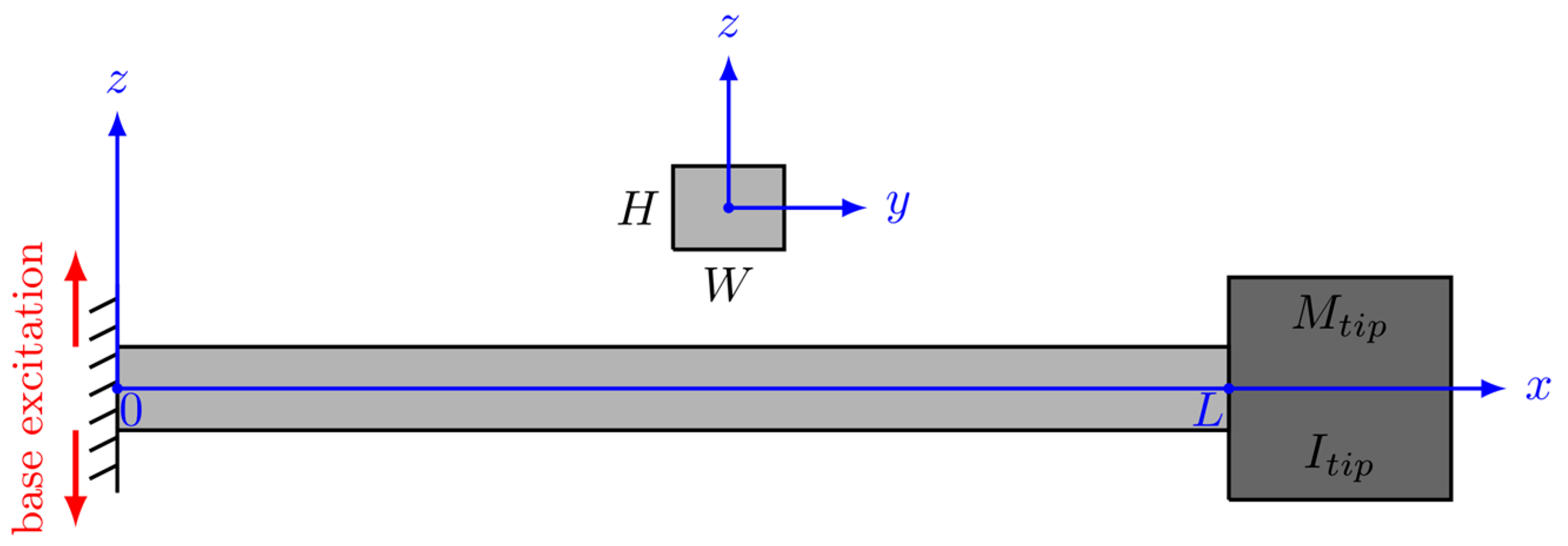
Figure 2.
Comparison between the analytical solution and the numerical approximation obtained using the Wynn-epsilon method for FVK oscillator with parameters : (a) Solution components corresponding to the initial condition ; (b) Solution components corresponding to the initial condition .
Figure 2.
Comparison between the analytical solution and the numerical approximation obtained using the Wynn-epsilon method for FVK oscillator with parameters : (a) Solution components corresponding to the initial condition ; (b) Solution components corresponding to the initial condition .
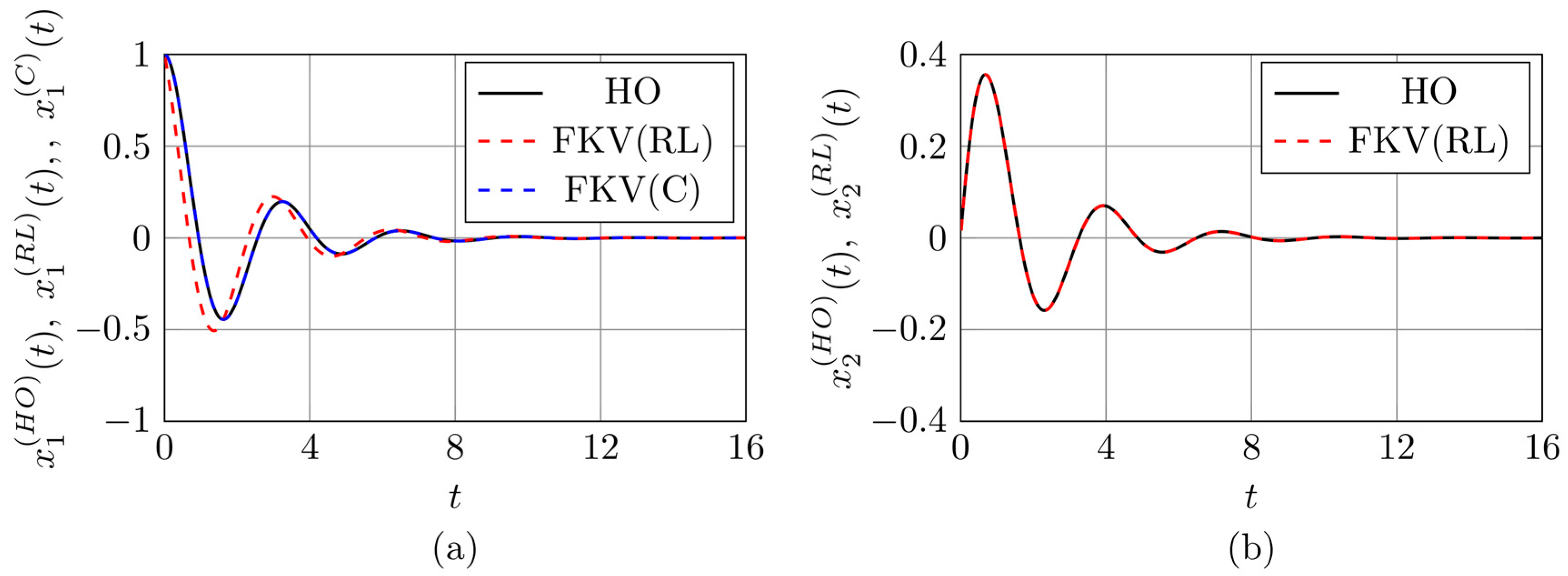
Figure 3.
Comparison between the analytical solution and the numerical approximation obtained using the Wynn-epsilon method for FVK oscillator with parameters : (a) Solution components corresponding to the initial condition ; (b) Solution components corresponding to the initial condition .
Figure 3.
Comparison between the analytical solution and the numerical approximation obtained using the Wynn-epsilon method for FVK oscillator with parameters : (a) Solution components corresponding to the initial condition ; (b) Solution components corresponding to the initial condition .
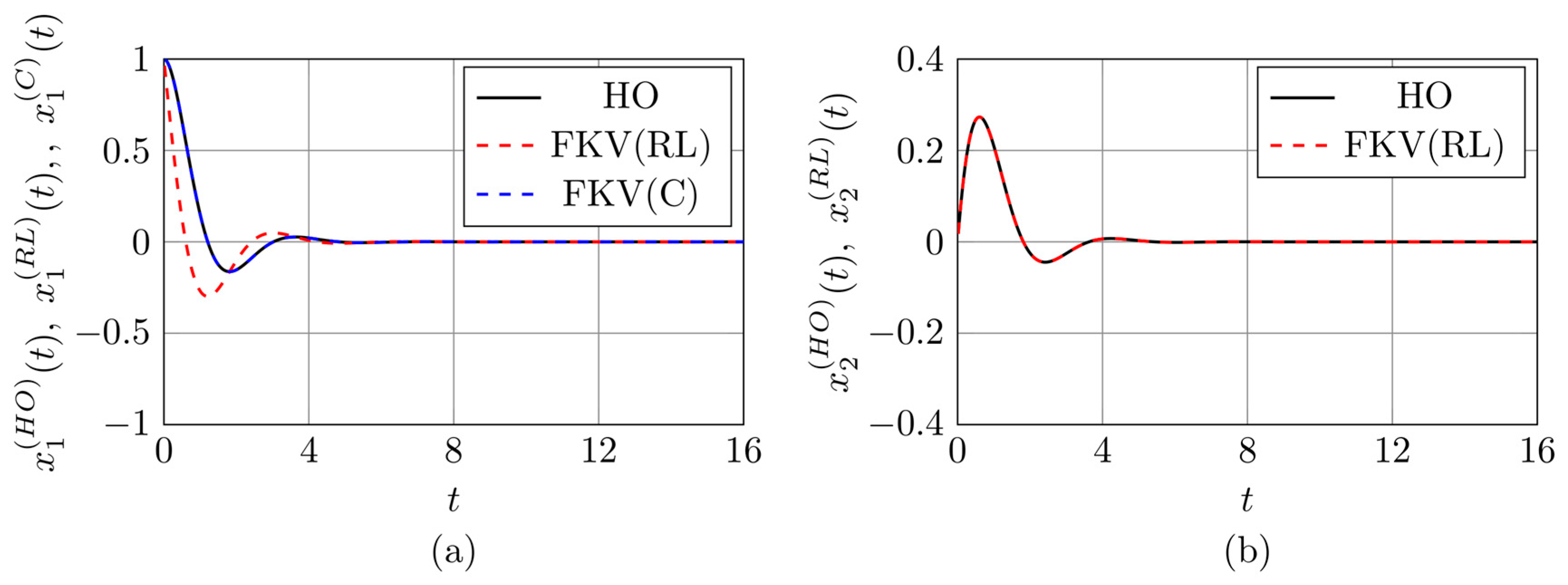
Figure 4.
Comparison between the analytical solution and the numerical approximation obtained using the Wynn-epsilon method for FVK oscillator with parameters : (a) Solution components corresponding to the initial condition ; (b) Solution components corresponding to the initial condition .
Figure 4.
Comparison between the analytical solution and the numerical approximation obtained using the Wynn-epsilon method for FVK oscillator with parameters : (a) Solution components corresponding to the initial condition ; (b) Solution components corresponding to the initial condition .
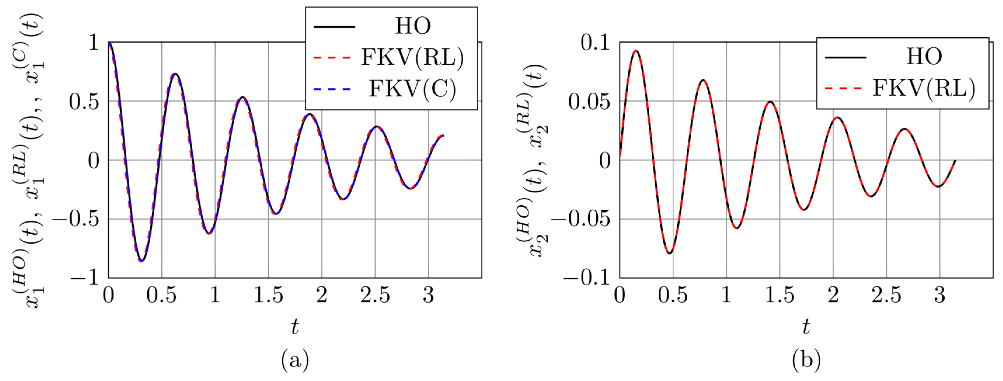
Figure 5.
Comparison between the exact solution and the Wynn-epsilon approximation of the fractional oscillator response for : (a): , , ; (b): , , . In both cases, the external forcing is defined by Eq. (18) with and .
Figure 5.
Comparison between the exact solution and the Wynn-epsilon approximation of the fractional oscillator response for : (a): , , ; (b): , , . In both cases, the external forcing is defined by Eq. (18) with and .
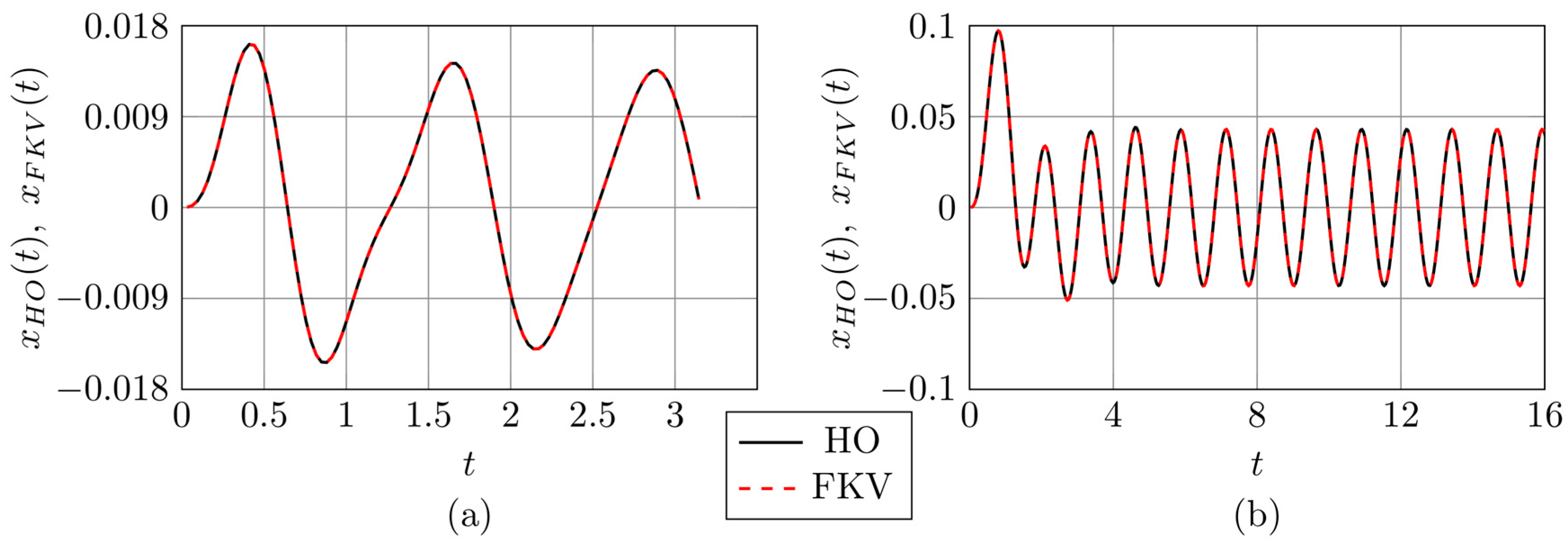
Figure 6.
Comparison between the components of the fractional and classical oscillator responses for the FKV oscillator with parameters : (a) displacement-related components; (b) velocity-related components.
Figure 6.
Comparison between the components of the fractional and classical oscillator responses for the FKV oscillator with parameters : (a) displacement-related components; (b) velocity-related components.
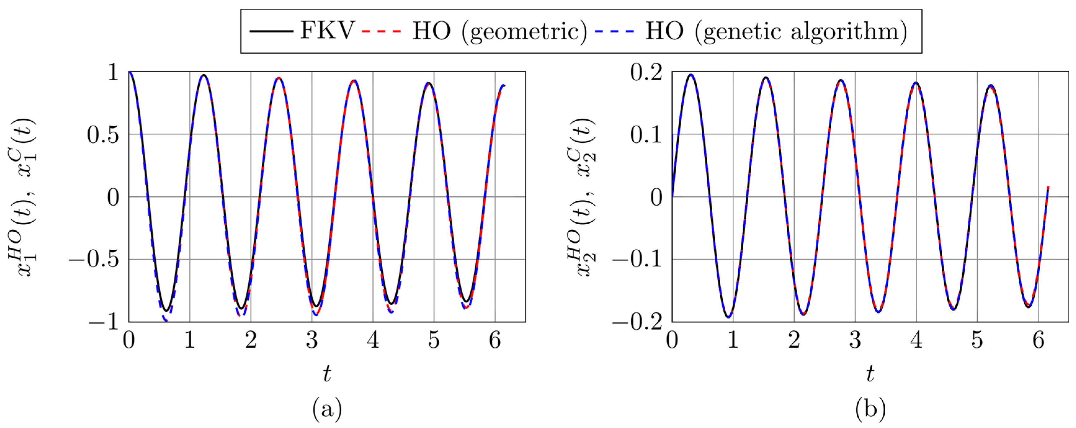
Figure 7.
Comparison between the components of the fractional and classical oscillator responses for the FKV oscillator with parameters : (a) displacement-related components; (b) velocity-related components.
Figure 7.
Comparison between the components of the fractional and classical oscillator responses for the FKV oscillator with parameters : (a) displacement-related components; (b) velocity-related components.
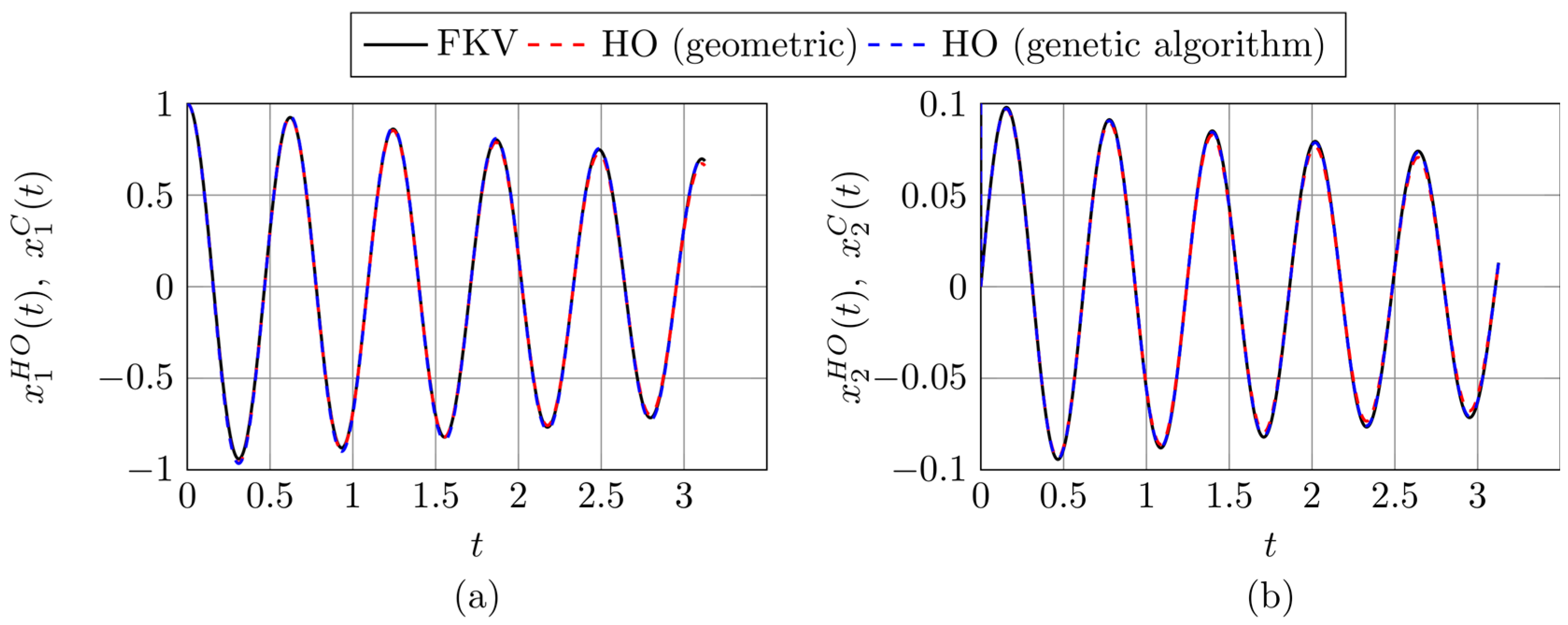
Figure 8.
Comparison between the components of the fractional and classical oscillator responses for the FKV oscillator with parameters : (a) displacement-related components; (b) velocity-related components.
Figure 8.
Comparison between the components of the fractional and classical oscillator responses for the FKV oscillator with parameters : (a) displacement-related components; (b) velocity-related components.
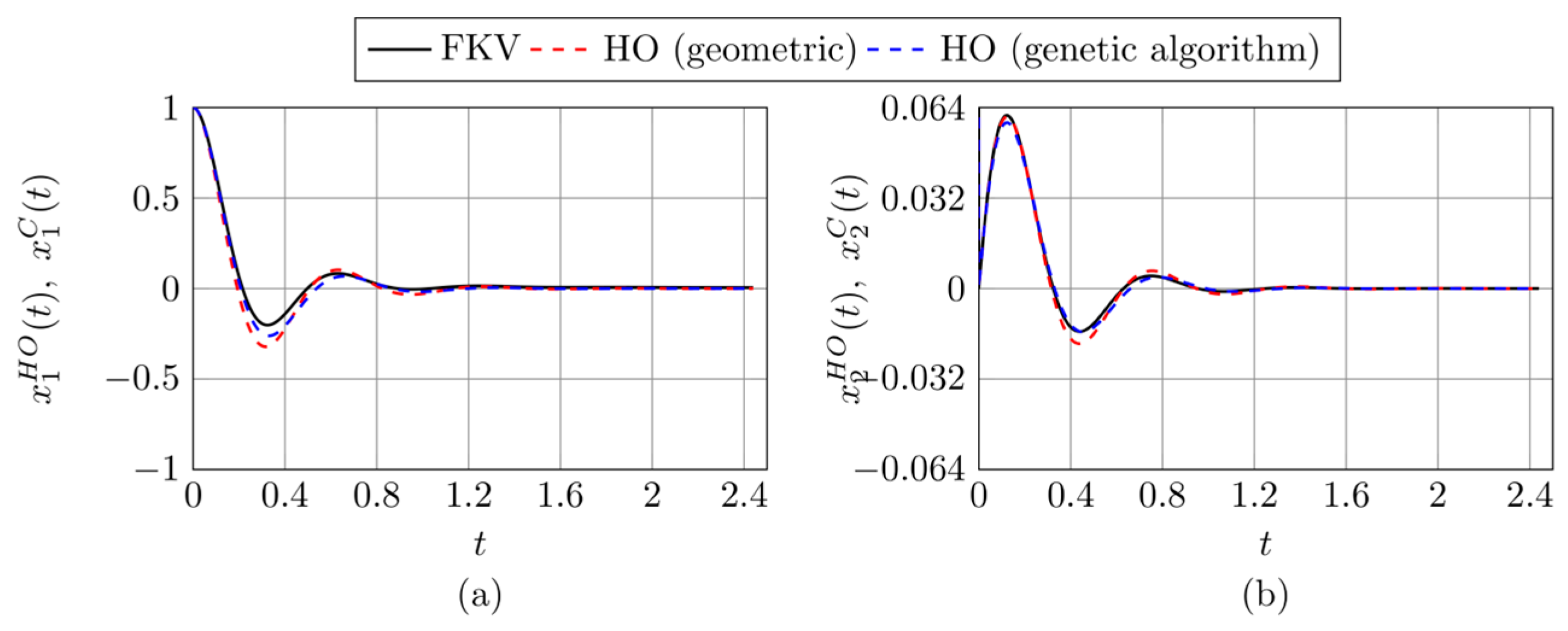
Figure 9.
Comparison between the components of the fractional and classical oscillator responses for the FKV oscillator with parameters : (a) displacement-related components; (b) velocity-related components.
Figure 9.
Comparison between the components of the fractional and classical oscillator responses for the FKV oscillator with parameters : (a) displacement-related components; (b) velocity-related components.
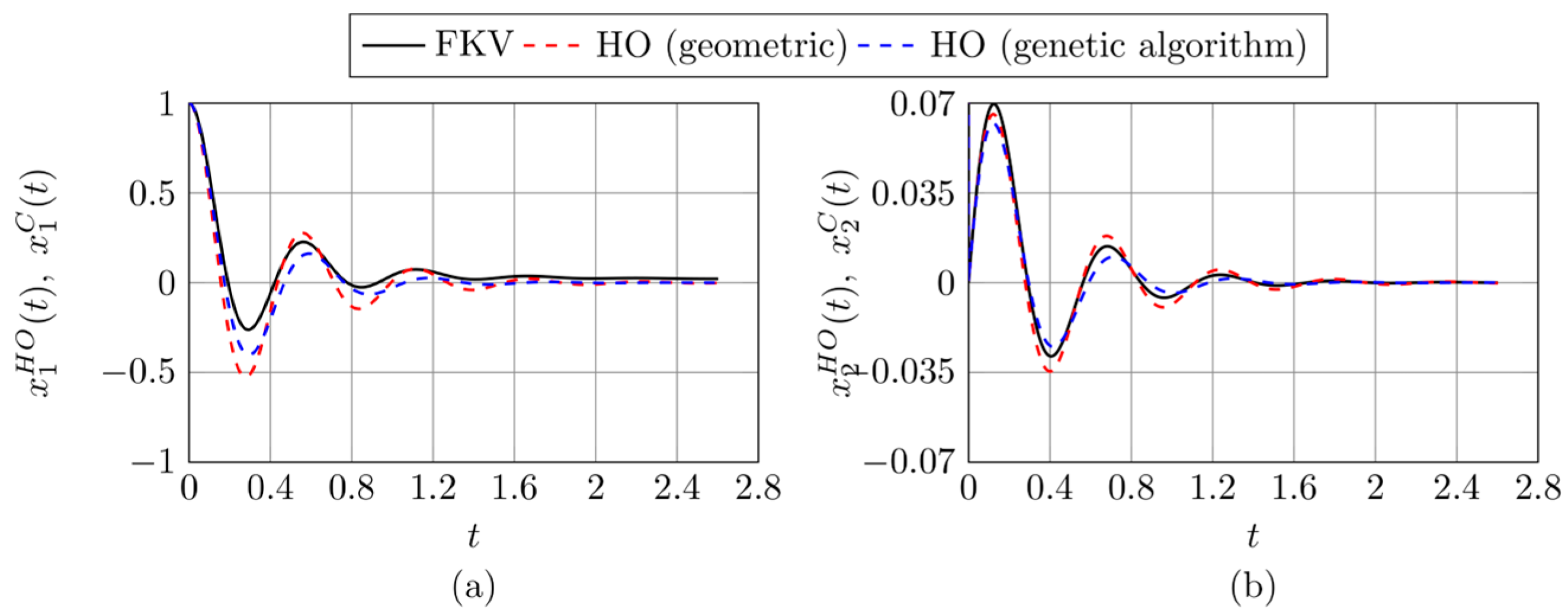
Figure 10.
Results for the FKV oscillator with parameters : (a) forcing frequency (resonance case); (b) forcing frequency (off-resonance case).
Figure 10.
Results for the FKV oscillator with parameters : (a) forcing frequency (resonance case); (b) forcing frequency (off-resonance case).
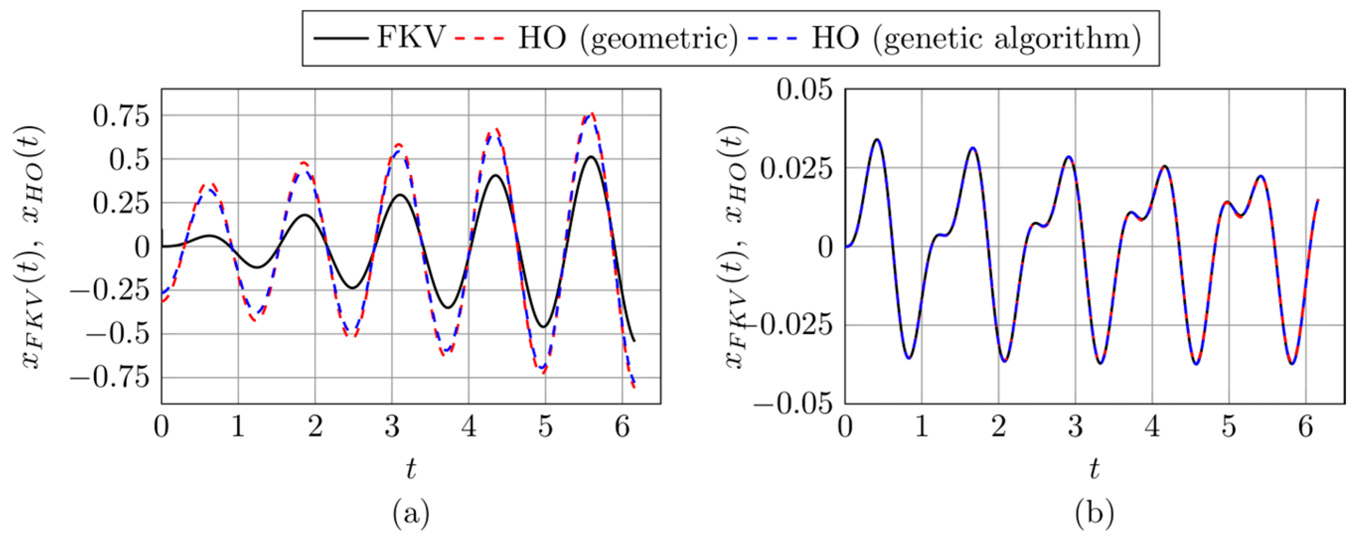
Figure 11.
Results for the FKV oscillator with parameters : (a) forcing frequency (off-resonance case); (b) forcing frequency (resonance case).
Figure 11.
Results for the FKV oscillator with parameters : (a) forcing frequency (off-resonance case); (b) forcing frequency (resonance case).
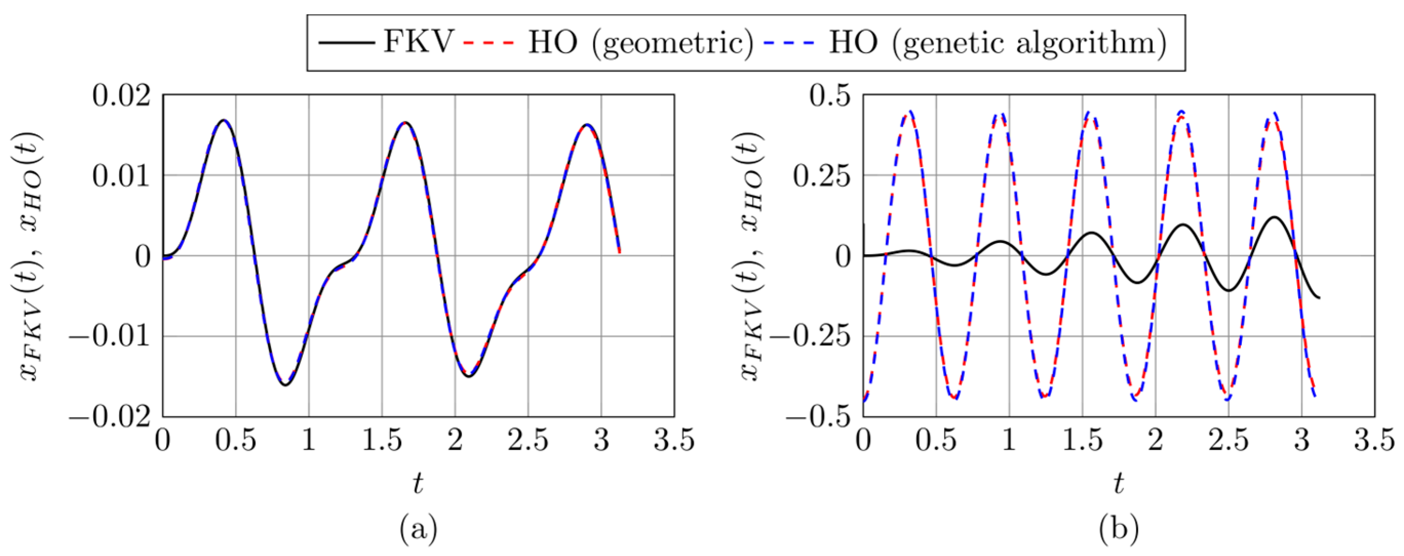
Figure 12.
Divergence coefficient as a function of the frequency ratio for two FKV oscillators: (a) ; (b) .
Figure 12.
Divergence coefficient as a function of the frequency ratio for two FKV oscillators: (a) ; (b) .
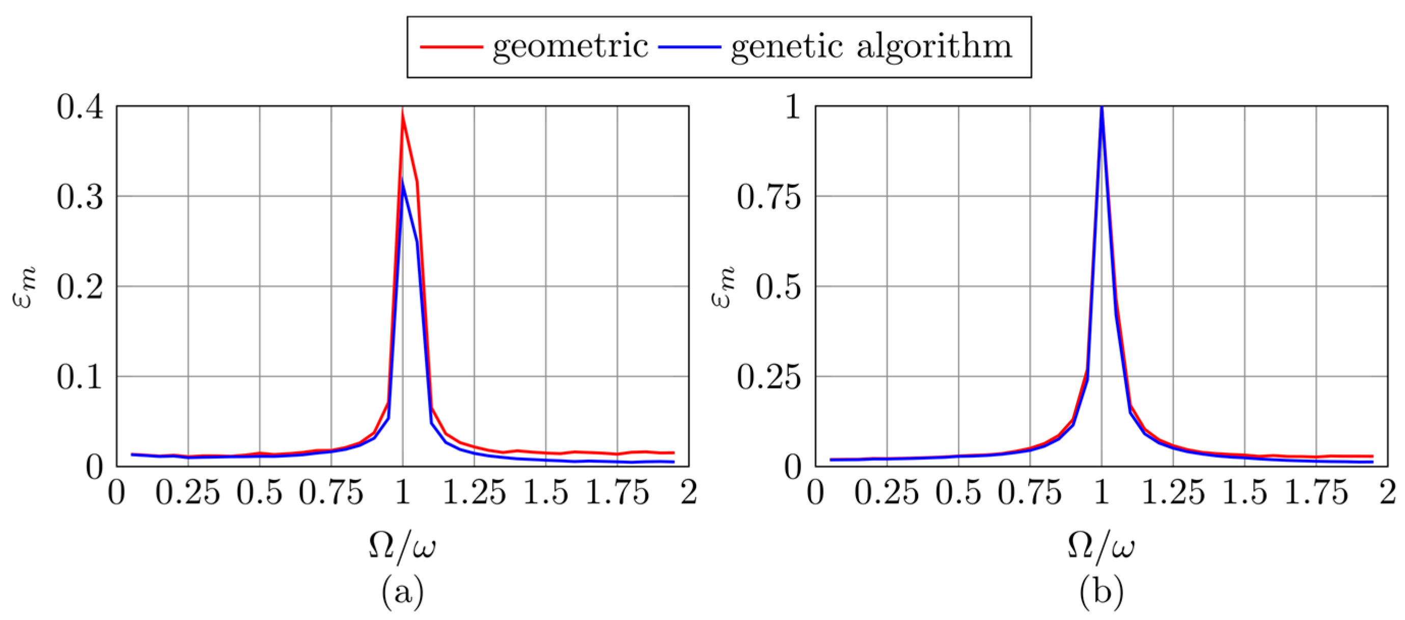

Table 1.
Comparison of harmonic oscillator parameters identified for various FKV oscillators using the geometric method and the genetic algorithm, along with the corresponding values of the divergence coefficient .
Table 1.
Comparison of harmonic oscillator parameters identified for various FKV oscillators using the geometric method and the genetic algorithm, along with the corresponding values of the divergence coefficient .
| FKV oscillator parameters | Geometric Approach | Genetic algorithm |
Disclaimer/Publisher’s Note: The statements, opinions and data contained in all publications are solely those of the individual author(s) and contributor(s) and not of MDPI and/or the editor(s). MDPI and/or the editor(s) disclaim responsibility for any injury to people or property resulting from any ideas, methods, instructions or products referred to in the content. |
© 2025 by the authors. Licensee MDPI, Basel, Switzerland. This article is an open access article distributed under the terms and conditions of the Creative Commons Attribution (CC BY) license (http://creativecommons.org/licenses/by/4.0/).
Copyright: This open access article is published under a Creative Commons CC BY 4.0 license, which permit the free download, distribution, and reuse, provided that the author and preprint are cited in any reuse.


