
Submitted:
11 April 2025
Posted:
14 April 2025
Read the latest preprint version here
Abstract
Traditional portfolio optimization techniques predominantly rely on the classical mean–variance framework introduced by Markowitz, which focuses on balancing expected returns against risk, typically measured by variance. However, in volatile and structur-ally unstable markets such as cryptocurrencies, this approach often fails to capture the full spectrum of uncertainty and diversification potential. This paper introduces an al-ternative methodology grounded in entropy, a fundamental concept in information theory that quantifies uncertainty and disorder. By incorporating entropy into the portfolio optimization process, we offer a more generalizable, distribution-free approach that enhances diversification and resilience.We develop and analyze three distinct en-tropy-based models: the maximum Shannon entropy model, the second-order entropy (Tsallis) model, and the maximum weighted Shannon entropy model. These formula-tions extend the traditional mean–variance approach by integrating nonlinear uncer-tainty measures, enabling a richer representation of investor preferences and asset in-terdependencies. Analytical solutions to the proposed models are derived using the method of Lagrange multipliers, ensuring mathematical rigor and interpretability.The proposed models are empirically validated using a portfolio composed of four leading cryptocurrencies—Bitcoin (BTC), Ethereum (ETH), Solana (SOL), and Binance Coin (BNB)—with market data from January to March 2025. The case studies demonstrate how entropy-based optimization leads to well-diversified portfolios, robust under market turbulence and heavy-tailed return distributions. Notably, the models facilitate dynamic adjustments in asset allocation in response to shifts in return–risk characteristics and entropy levels.
This study contributes to the ongoing generalization of portfolio theory by positioning entropy as both a diversification enhancer and a structural risk measure. It provides theoretical insight, practical tools for asset allocation in high-volatility environments, and paves the way for future research in entropy-driven financial optimization frameworks.
Keywords:
Shannon Entropy
; Second-Order Entropy
; Weighted Entropy
; Portfolio Optimization
; Cryptocurrency Market
; Mean–Variance–Entropy Model
; Risk Diversification
1. Introduction
Portfolio optimization represents a foundational problem in modern finance, concerned with determining the optimal allocation of an investor’s wealth across a selection of assets in order to achieve an appropriate balance between expected return and risk exposure. The classical approach to this challenge is encapsulated by the mean–variance model proposed by Markowitz (1952) [16], which utilizes historical return data, variances, and covariances between asset returns to construct efficient portfolios based on first- and second-order statistical measures. Within this framework, the primary objective is to either maximize expected return for a given level of risk or minimize risk for a targeted return.
In response to the limitations of the classical framework—particularly its reliance on normally distributed returns and sensitivity to estimation errors—numerous alternative models have emerged. These include refinements of the risk measure itself: Konno and Yamazaki [14] introduced the mean-absolute deviation model, while Speranza [23] proposed the semi-absolute deviation approach. Semivariance-based models, as developed by King and Jensen [13], King [12], and later refinements by Markowitz and collaborators, focus more accurately on downside risk. Meanwhile, Hamza and Janssen [7] extended the scope of large-scale optimization through asymmetric risk functions and separable programming formulations.
Additional developments have sought to account for real-world market conditions such as transaction costs, liquidity constraints, and market frictions. Notable contributions in this area include the works of Pogue [19], Rudd and Rosenberg [20], and Yoshimoto [26], who introduced V-shaped cost functions and nonlinear optimization techniques. Despite these innovations, many empirical studies—such as those conducted by DeMiguel et al. [3,4]—highlight that complex optimization models do not always outperform naive strategies like the equally-weighted portfolio, especially when facing estimation uncertainty and limited sample sizes.
Within this broader context, diversification remains a key determinant of portfolio performance. In recent years, entropy has emerged as a powerful tool for enhancing and measuring diversification within portfolio theory. As a measure of uncertainty or disorder, entropy provides a flexible and distribution-free alternative to variance. Shannon's pioneering work [21] laid the mathematical foundation for entropy as a quantifier of information content, which was later adapted for financial applications by researchers such as Yager [25], Wang and Parkan [24], and Philippatos and Wilson [17,18]. These studies emphasized entropy’s ability to capture more nuanced forms of risk and portfolio dispersion, especially when return distributions deviate from normality or when market data are incomplete or noisy.
Empirical applications have further supported entropy’s relevance in finance.
Simonelli [22] demonstrated that entropy-based models outperform traditional deviation-based measures in capturing portfolio uncertainty. Jiang et al. [10,27] and Ke and Zhang [11] extended these findings to large-scale optimization problems, incorporating entropy into robust decision-making frameworks. In parallel, Zhou [29] underscored the growing acceptance of entropy in financial modeling, highlighting its application across diverse domains—from energy procurement to digital asset management. Notably, recent studies have employed entropy-based methods in the cryptocurrency sector, where market volatility, nonlinear correlations, and non-normal return distributions are particularly pronounced [8].
Building on this extensive body of literature, the present paper introduces three entropy-enhanced models for portfolio optimization: the maximum Shannon entropy model, the second-order (Tsallis) entropy model, and the maximum weighted Shannon entropy model. These models enrich the traditional mean–variance paradigm by incorporating nonlinear and information-theoretic dimensions of uncertainty. Theoretical derivations based on the method of Lagrange multipliers are presented, followed by a series of empirical case studies using market data from January to March 2025. The findings demonstrate that entropy-based optimization improves diversification, mitigates concentration risk, and offers structurally robust allocations—particularly in the highly volatile environment of cryptocurrency markets.
The remainder of the paper is organized as follows: Section 2 introduces the entropy-based optimization models and their analytical formulations. Section 3 presents the numerical results derived from case studies involving cryptocurrency portfolios. Section 4 concludes the study by summarizing the key findings and suggesting avenues for future research
2. Materials and Methods
2.1. Fundamentals of portfolio entropy
2.1.1. Entropy Approach to a Portfolio
Entropy is a foundational concept designed to quantify the degree of randomness and uncertainty inherent in a system. Originally introduced in thermodynamics and later extended to information theory, entropy has become a central metric of disorder, with wide-ranging applications in fields such as econometrics, finance, and statistical mechanics. In the context of dynamic systems, entropy provides a rigorous framework for measuring unpredictability: a system with zero entropy reflects perfect determinism, whereas higher entropy values indicate increasing levels of uncertainty and structural complexity [6,21].
Over time, the theoretical grounding and interdisciplinary relevance of entropy have been expanded by numerous landmark contributions. Boltzmann’s formulation of statistical mechanics laid the foundation by conceptualizing entropy as a measure of physical disorder. Shannon subsequently formalized entropy in the context of information theory, defining it as the expected value of the information content of a message. Building on this idea, researchers such as Wiener, Khinchin, Faddeev, Rényi, Tsallis, Guiasu, and Onicescu [28] extended the concept both mathematically and conceptually, paving the way for applications far beyond the physical sciences—including finance and portfolio theory.
A major milestone in this evolution was Jaynes’s introduction of the principle of maximum entropy [9], which posits that, in the presence of incomplete or partial information, the probability distribution that maximizes entropy represents the most unbiased and objective estimate. This principle has since become a cornerstone of probabilistic inference and rational decision-making under uncertainty [5,15].
In contemporary financial theory and portfolio management, entropy is increasingly acknowledged as a robust and flexible tool for evaluating diversification and managing risk. Compared to traditional variance-based metrics, entropy provides a more general and nonlinear approach to quantifying portfolio uncertainty. Shannon’s original entropy model laid the groundwork for future refinements, including Yager’s application of the maximum entropy principle to decision-support systems [25]. Wang and Parkan [24] advanced this line of inquiry by developing a linear entropy model, while Philippatos and Wilson [17,18] emphasized entropy’s superiority over variance as a risk metric, particularly in cases involving non-normal or incomplete data.
More recently, Jiang et al. [2,11,27] proposed a maximum entropy-based portfolio optimization model that effectively integrates entropy into asset allocation strategies. These contributions collectively underscore the growing importance of entropy in financial modeling, offering a powerful and generalizable methodology for uncertainty quantification, strategic diversification, and portfolio construction [28].
2.1.2. Empirical Approach to the Entropy of a Portfolio
If we refer to the financial environment, in particular to portfolio theory, we can observe the following (We will denote the portfolio formed from n assets with
1. If a certain action "" has a high degree of investment security (low risk and high profit), then it is natural to invest a large proportion in this asset, i.e. , therefore , i.e. , and the portfolio has the structure
2. If the portfolio is formed from assets about which almost nothing is known, then it is natural (the diversification principle) to invest equal proportions in each of the assets. Therefore, the portfolio has the structure , and
Remark 1: As a measure of portfoliouncertainty, we should consider a weighted average of the perception of uncertainty of each asset, whererepresents the perception of uncertainty of the investment in the i-th asset.
Remark 2: If the proportionincreases creases, the uncertainty decreases, signal magnitude(respectively of the uncertainty in the investment) decreases. Therefore, we have that.
Remark 3: From an empirical point of view, the perception of a signal is found to be proportional to log(signal). In our case, we will have
Combining the above observations, we can consider as a measure of uncertainty of a portfolio the function
Remark 4: The function is concave. Therefore, according to Jensen's inequality, has the maximum value when
2.1.3. Axiomatic Approach to Portfolio Entropy
The empirical approach to entropy already suggests two essential conditions that it must satisfy, namely:
maximum, where represents the entropy of portfolio x.
On the other hand, it is clear that depends only on the investments actually made, , and the order of the investments is also not important, i.e., . In conclusion, if we define as the maximum of all portfolio entropies with effective investments, then satisfies the following conditions:
Axiom I. 1) (reformulation of condition C₂)
2) f is strictly increasing
3) f(1) = 0 (reformulation of condition C₁)
Axiom II. (the function is of logarithmic type)
Axiom III. The function is continuous
Axiom IV. where
As a result of the existing studies in this direction in the specialized literature, we can present the following result:
Theorem: If the function H satisfies Axioms I-IV, then , for a certain value of the constant C, where
2.2. Maximum Entropy Models to Portfolio Optimization
2.2.1. Maximum Shannon entropy portfolio model
Shannon entropy, originally developed within the field of information theory to address communication system challenges, has since evolved into a powerful and versatile tool across multiple disciplines, including finance and portfolio management. As a fundamental measure of uncertainty, Shannon entropy offers a rigorous mathematical framework for quantifying disorder and randomness in complex systems. In financial contexts, it is increasingly recognized as a robust alternative to traditional risk measures such as variance and standard deviation. Among the early proponents of this perspective, Simonelli [22] emphasized the enhanced ability of entropy-based models to capture the multifaceted nature of portfolio uncertainty and diversification, outperforming conventional deviation-based metrics. This view was further supported by Philippatos and Wilson [17,18], who formally established the theoretical link between Shannon entropy and financial risk. By incorporating entropy as a diversification metric, investors gain the ability to systematically evaluate the uncertainty embedded in different asset allocations, contributing to more resilient and structurally balanced portfolios [22].
The integration of Shannon entropy into portfolio theory has led to the development of advanced optimization frameworks that transcend the inherent limitations of mean-variance models. Unlike classical approaches that rely on distributional assumptions and linear measures of dispersion, entropy-based methods are non-parametric and distribution-free. This flexibility is particularly advantageous in volatile and nonlinear market environments, where asset returns frequently deviate from normality. As a result, entropy-driven strategies have garnered increasing attention from both researchers and practitioners seeking robust, adaptive, and theoretically sound tools for financial decision-making. In this context, portfolio optimization is reframed as the problem of maximizing Shannon entropy—striking an optimal balance between diversification and risk mitigation. By constructing portfolios that maximize entropy, investors can reduce concentration risk and promote allocation uniformity, thereby enhancing structural stability. This probabilistic approach to uncertainty enables the design of investment strategies that are inherently more resilient to turbulent and unpredictable market conditions.
The following section presents the formal mathematical formulation of this entropy-based portfolio optimization model.
Shannon defined entropy as the amount of information available to a system of states with the probability vector ,. Explicitly, Shannon entropy has the form is defined by , where is the weight of asset in the portfolio.
Shannon entropy is used to optimize a portfolio by replacing variance with entropy in the known optimization model (mean-variance). Thus, we obtain the model:
where is the expected average return of the portfolio and the level is assumed by the investor.
Using the Lagrange multipliers method, we obtain:
The first-order conditions become:
Because we have that , we obtain , we rewrite in (#) and obtain
, i = where the two multipliers verify the relationships, given the constraints of the optimization problem, where we replaced with the value obtained above
2.2.2. Maximum second order entropy portfolio model
In this section, we develop a portfolio optimization model that incorporates return, second-order entropy, and variance as core components. The model seeks to maximize a weighted combination of expected return and entropy, subject to a risk constraint expressed via variance. This approach enhancesdiversification and liquidity, while ensuring that the overall risk remains within an acceptable level, as defined by the investor.
Tsallis Entropy : where
(For in Tsallis entropy we obtain the informational entropy introduced by O.0nicescu, given by )
Second order entropoy (Tsallis with ):Remarks:
1. For a given portfolio, this kind of entropy measures the correlation degree of the assets from the portfolio ()
2. A lower entropy implies greater concentration (lower diversification), whereas a higher entropy reflects greater diversification, which may contribute positively to portfolio liquidity
Optimization Problem Formulation
where
is the expected average return of the portfolio and the level,
is assumed by the investor
Solving the portfolio optimization problem
Using the Lagrange multipliers method, we obtain:
The first-order conditions become:
Because we have that , we
Replacement relationship (*) we get
+ )+ where the two multipliers verify the relationships, given the constraints of the optimization problem, where we replaced with the value obtained above
2.2.3. The Maximum Weighted Shannon Entropy Portfolio Model
We begin by introducing the concept of weighted entropy, as originally proposed by Guiasu, which extends the classical Shannon entropy by incorporating a vector of strictly positive weights. The weighted entropy is defined as follows:
Guiasu defined entropy as the amount of information available to a system of states with the probability vector ,. Explicitly, Guiasu entropy has the form , where > 0 represent the weights associated with each probability component nd. This formulation allows for a more flexible representation of uncertainty by accounting for the relative importance or influence of each asset in the portfolio.
The proposed optimization framework builds upon the principle of maximum entropy, incorporating both mean and variance constraints to ensure consistency with classical portfolio theory. The portfolio optimization problem can thus be reformulated as the maximization of the weighted Shannon entropy subject to constraints on the expected return and variance. Formally, we define the problem as follows:
where
is the weight of asset i in portfolio,
E is the desired expected return of the portfolio,
the desired portfolio variance,
reflects the importance of asset i
This approach represents an alternative to the classical Markowitz framework, offering a richer modeling of uncertainty and potential for enhanced portfolio diversification through entropy maximization.
Using the Lagrange multipliers method, we obtain:
The first-order conditions become:
+ + (#)
Because , we obtain , we rewrite in (#) and obtain
, i=, where the two multipliers verify the relationships, given the constraints of the optimization problem, where we replaced with the value obtained above
2.3 Case studies
In this section, we apply the maximum second-order entropy model to a portfolio composed of major cryptocurrencies. The data used in the analysis reflects market activity from January to March 2025, with weekly returns collected from publicly available cryptocurrency trading platforms. Our goal is to test the practical applicability of the entropy-based optimization model and to demonstrate its ability to generate well-diversified portfolios under real market conditions.
The results presented below are derived using the second-order entropy function and reflect optimal weight allocations and associated entropy values under different portfolio compositions.
Case n=2:Portfolio Optimization with Two Cryptocurrencies
We first consider a simplified portfolio comprising two major cryptocurrencies: Bitcoin (BTC) andEthereum (ETH). Using the second-order entropy model and the data collected from Q1 2025, we computed the optimal allocation that maximizes the entropy function under standard return and variance constraints.
Using historical price data, we calculate statistics:
E₁ = 0.0565, σ₁² = 0.46; E₂ = 0.0133, σ₂² = 1; σ₁₂ = 0.203. Based on these inputs, we have model:
max (-x₁²-x₂²)
Using the formulas presented in the section 2.2 obtain
) + x₁ =γ₁/2(0.0565-0.0349) + γ₂/2(0.033-0.8)/2) + 0.5 = 0.01γ₁ - 0.18γ₂ + 0.5
x₂ = γ₁/2(0.0133-0.0349)+γ₂/2)(0.775-0.8)/2)) + 0.5 = -0.01γ₁+0.18γ₂+0.5
where the two multipliers γ₁and γ₂ verify relations :
x₁⋅ 0.0565 + x₂⋅ 0.0133 = 0.05
x₁⋅ 0.033 + x₂⋅ 0.0775 = 0.1,
or
(0.01γ₁ - 0.18γ₂+ 0.5)⋅0.0565 + (-0.01γ₁+ 0.18γ₂ + 0.5)⋅0.0133 = 0.05
(0.01γ₁ - 0.18γ₂+ 0.5)⋅0.033 + (-0.01γ₁+ 0.18γ₂ + 0.5)⋅0.775 = 0.1,
┊ or
0.0055γ₁ - 0.0077γ₂ + 0.03 = 0.05
- 0.0074γ₁ + 0.1335γ₂ + 0.4 = 0.1
We will solve the sistem and we have γ₁ = 0.53155 and γ₂ = -2. 2177
We obtain x₁ = 0.905 and x₂ = 0.095
This result indicates that, under the given preferences and market conditions, the optimal portfolio heavily favors Bitcoin (BTC), allocating approximately 90.5% of the capital to BTC and only 9.5% to ETH.
Case n=3Portfolio Optimization with Three Cryptocurrencies
In this section, we consider a portfolio composed of three major cryptocurrencies: Bitcoin (BTC), Ethereum (ETH), and Solana (SOL), observed over the period 18 January 2025 – 21 March 2025. The optimization system was solved numerically using MATLAB, We have our inputs and we are going to use maximum second order entropy portfolio model. We obtain :
max (- x₁² - x₂² - x₃²)
x₁⋅0.0565 + x₂⋅0.0133 + x₃⋅0.0755 = 0.05
x₁⋅0.033 + x₂⋅0.775 + x₃⋅0.105 = 0.1,
x₁ + x₂ + x₃ = 1
Using the formulas presented in the section 2 obtain
x₁ = γ₁/2 (0.0565 - 0.048) +γ₂/2(0.033 - 0.3) + 0.33 = 0.004γ₁ - 0.134γ₂ + 0.33
x₂ = γ₁/2(0.0133-0.048) + γ₂/2(0.775-0.3) + 0.33 = -0.017γ₁ + 0.232γ₂ + 0.33
x₃ = γ₁/2(0.0755-0.048) + γ₂/2(0.105-0.3) + 0.33 = 0.013γ₁ - 0.098γ₂ + 0.33
where the two multipliers γ₁ and γ₂ verify relations :
(0.004γ₁-0.134γ₂+0.33)⋅0.0565+(-0.017γ₁+0.232γ₂+0.33)⋅0.0133+(0.013γ₁-.098γ₂+0.33)⋅0.0755 = 0.05
(0.004γ₁-0.134γ₂+0.33)⋅0.033+(-0.017γ₁+0.232γ₂+0.33)⋅0.775+(0.013γ₁-0.098γ₂+0.33)⋅0.105
= 0.1,or
0.003γ₁ - 0.012γ₂ + 0.048 = 0.05
-0.036γ₁ + 0.072γ₂ + 0.3 = 0.1,
we have γ₁ = 10. 444,γ₂ = 2. 444 and we obtain x₁ = 0.05 , x₂ = 0.72, x₃ = 0.23
Compared to the two-asset case, the three-asset configuration produced a more balanced and diversified portfolio. The entropy value increased significantly, indicating an improvement in diversification. The numerical solution favors Ethereum (72%) over Bitcoin (5%) and Solana (23%), suggesting that, under the given statistical assumptions, ETH offers the most efficient return-risk combination. This shift highlights the sensitivity of entropy-based optimization to the underlying input data and the ability of the model to capture subtle structural differences across assets. Moreover, the enhanced entropy level suggests greater portfolio resilience under dynamic market conditions
Case n = 4Portfolio Optimization with For Cryptocurrencies
In this section, we consider a portfolio composed of four major cryptocurrencies—Bitcoin (BTC), Ethereum (ETH), Solana (SOL), and Binance Coin (BNB)—traded actively during the period January–March 2025. These digital assets represent a wide range of use cases and exhibit significant market capitalization, liquidity, and volatility, making them relevant for a realistic portfolio optimization scenario in the current crypto landscape.
We apply the maximum weighted Shannon entropy portfolio model for portfolio selection. This approach emphasizes diversification by minimizing portfolio concentration, i.e., maximizing entropy, while simultaneously imposing constraints related to expected return and overall risk exposure.
The model we use is defined as follows:
where
is the weight of asset i in portfolio,
E is the desired expected return of the portfolio.We choose E = 0,4
the desired portfolio variance. We choose = 170
reflects the importance of asset i. We choose = = 1
These constraints simulate a scenario where the expected return of the portfolio must reach a minimum target (e.g., 0.4), while a weighted measure of asset riskinterpreted here as a proxy for volatility, market exposure, or price confidence—is bounded by 170 units.
This structure is consistent with historical performance patterns observed during Q1 2025 across the selected crypto assets. The optimization system was solved numerically using MATLAB, which all owed for accurate handling of symbolic constraints and nonlinear systems.
We obtained the optimal asset allocation within the entropy-based
framework. The resolution process involved simultaneously satisfying the conditions of expected return, variance threshold, and total portfolio allocation. The solution yields the following asset weights:
x1 = 0.21(BTC),
x2 = 0.22(ETH),
x3 = 0.29(SOL),
x4 = 0.28(BNB)
These results reflect a relatively balanced distribution of capital across the
four assets, with a slightly higher allocation toward Solana and Binance Coin. This may indicate a superior return-to-volatility ratio for these tokens during Q1 2025, or a better informational weight under the entropy framework. Notably, the allocation is not dominated by a single asset, which confirms that the entropy model naturally leads to diversification, even under strong constraints.
Furthermore, this outcome underlines the core strength of the entropy-
based approach: its ability to integrate multiple dimensions of portfolio quality—namely, return, risk, and diversification—into a unified and mathematically consistent optimization scheme. While traditional models may struggle under high volatility and non-normal return distributions (characteristic of crypto markets), the entropy model adapts well due to its distribution-independent structure and flexible treatment of uncertainty.
In summary, the entropy-based allocation obtained herein demonstrates
not only mathematical feasibility but also practical relevance for crypto investors seeking resilient portfolio structures in volatile market contexts. The result confirms that entropy can serve as both a theoretical and operational pillar in modern portfolio construction, particularly in digital asset environments.
3. Results and Discussions
The numerical results for both portfolio configurations—two assets (BTC and ETH) and three assets (BTC, ETH, and SOL)—are summarized in Table 1. The corresponding asset allocations, shown in Figure 1, highlight the structural transformation induced by the entropy-based optimization process. Specifically, the shift from a highly concentrated allocation (90.5% BTC) in the two-asset case to a more distributed configuration in the three-asset portfolio (72% ETH, 23% SOL, and 5% BTC) illustrates how entropy promotes diversification as more viable assets are introduced.
The observed increase in entropy from Case 1 to Case 2 is not merely a numerical side effect, but rather a reflection of entropy’s role as a structural force within the optimization process. Entropy acts as more than a passive term in the objective function—it actively regulates the portfolio’s composition by discouraging excessive concentration in any single asset. In this sense, entropy introduces a "soft constraint" that balances the optimizer’s tendency to overweight high-return assets with the need for robustness and adaptability. From a practical standpoint, this mechanism is particularly valuable in the cryptocurrency domain, where asset correlations are volatile, return distributions are non-normal, and structural shifts occur frequently. Entropy serves not only as a statistical indicator of uncertainty, but also as a strategic hedge against systemic risk and overexposure to single-asset dominance.. Moreover, its integration into the optimization process enables a more adaptive response to evolving market dynamics, making it particularly valuable in volatile and information-sparse environments such as the cryptocurrency sector .Given the volatile and structurally unstable nature of the cryptocurrency market, entropy-based models provide a more realistic framework for portfolio optimization than classical variance-based approaches.
This approach also presents potential use cases in institutional settings. For example, entropy-based allocation mechanisms could inform the construction of crypto indexes, stablecoin baskets, or managed digital asset funds. The model’s ability to integrate return optimization with diversification logic makes it especially relevant for portfolio managers navigating the high-volatility landscape of digital finance. Furthermore, the analytical tractability of second-order entropy facilitates its application in rule-based, automated investment systems. Ultimately, the results confirm that entropy is not merely a measure of diversification but a foundational element in shaping resilient, data-driven portfolios.
The entropy-driven allocations reflect a strategic compromise between return concentration and structural stability—providing a flexible framework that can adapt to evolving market dynamics
Table 1 summarizes the portfolio weights and entropy contributions for both configurations. As expected, the n = 2 portfolio displays strong concentration in BTC, while the n = 3 case reveals a more diversified structure with greater entropy.
Figure 1 provides a visual comparison of asset allocations in both cases, clearly illustrating how the inclusion of an additional asset reshapes the portfolio and enhances its diversification profile.
The application of the maximum weighted Shannon entropy model to a cryptocurrency portfolio consisting of BTC, ETH, SOL, and BNB over the period January–March 2025 yielded a diversified and balanced allocation. The model was solved under constraints of expected return E = 0.4, total variance 170, and uniform informational weights ui=1.The computed asset weights were as follows: = 0.21(BTC),= 0.22(ETH), = 0.29(SOL), = 0.28(BNB).These allocations satisfy the imposed constraints and reflect realistic investment decisions aligned with market behavior during the selected period. The model’s outcome suggests a mild preference for SOL and BNB, possibly due to their stronger return-risk tradeoff or favorable entropy-driven characteristics. Importantly, the portfolio avoids concentration in a single asset, fulfilling the principle of diversification embedded in the entropy criterion.
Figure 2 provides a visual comparison of asset allocations in case n = 4
The results validate the effectiveness of the entropy-based optimization approach in volatile environments such as crypto markets. In contrast to classical mean-variance portfolios, the entropy-based solution demonstrates robustness against overfitting and sensitivity to distributional assumptions. The analytical tractability of the model, combined with its flexibility, supports its applicability in real-world investment strategies, particularly when information asymmetry or market uncertainty is high
4. Conclusions
This paper has introduced a comprehensive entropy-based approach to portfolio optimization, addressing the limitations of traditional variance-centered models. By leveraging entropy as a core criterion, the models developed in this study provide a more general, flexible, and robust framework for asset allocation—particularly within high-volatility environments such as the cryptocurrency market. Three distinct entropy formulations were explored: the maximum Shannon entropy model, the second-order (Tsallis) entropy model, and the maximum weighted Shannon entropy model. Each model demonstrated its ability to enhance diversification, balance return-risk tradeoffs, and generate allocations that are less prone to concentration.
Through a series of empirical case studies involving portfolios with two, three, and four cryptocurrencies, the models were validated on real-world data from Q1 2025. The findings reveal key structural advantages of entropy-based optimization. Notably, the second-order entropy model efficiently captures inter-asset relationships and promotes risk-balanced distributions, while the weighted Shannon entropy model allows the integration of informational relevance into allocation decisions. These mechanisms collectively contribute to portfolio resilience under unstable market conditions and information asymmetry. The entropy-driven allocations reflected a strategic compromise between expected return, diversification, and robustness, producing solutions that align with theoretical insights and practical constraints. Moreover, the mathematical tractability of the models, ensured through Lagrangian optimization, offers implementation potential in algorithmic, rule-based, or automated investment settings.
This study contributes to the evolving literature on portfolio theory by demonstrating that entropy not only serves as a theoretical proxy for diversification, but also functions as a structural guide for portfolio construction. Entropy’s distribution-free nature, coupled with its capacity to measure uncertainty holistically, makes it particularly suitable for environments where return distributions deviate from normality and data quality is inconsistent.
Future research directions include the incorporation of dynamic entropy formulations, multi-period optimization horizons, and extensions to account for real-world factors such as transaction costs, liquidity constraints, and regulatory limits. Additional empirical testing across asset classes and emerging markets may further validate the generalizability and operational value of entropy-based portfolio models in diverse investment context
References
- Alexander, G. J., & Baptista, A. M. (2002). Economic implications of using a mean-VaR model for portfolio selection: A comparison with mean-variance and mean-conditional value-at-risk. Journal of Economic Dynamics and Control, 26(7–8), 1159–1193. https://experts.umn.edu/en/publications/economic-implications-of-using-a-mean-var-model-for-portfolio-sel.
- Chang, C., Chen, Y., & Liu, P. (2022). Robust cryptocurrency portfolio optimization using entropy measures under extreme volatility. Financial Innovation, 8, 34.
- DeMiguel, V., Garlappi, L., & Uppal, R. (2009). Optimal versus naive diversification: How inefficient is the 1/N portfolio strategy? Review of Financial Studies, 22(5), 1915–1953.
- DeMiguel, V., Garlappi, L., Nogales, F. J., & Uppal, R. (2009). A generalized approach to portfolio optimization: Improving performance by constraining portfolio norms. Management Science, 55(5), 798–812.
- Elsheikh, A., & Egret, J. (2021). Portfolio selection under entropy and higher-order moments: A new hybrid optimization model. Annals of Operations Research, 303, 511–532.
- Guiasu, S. (1971). Information Theory with Applications. McGraw-Hill.
- Hamza, K., & Janssen, J. (1998). A separable programming approach to portfolio selection with transaction costs and constraints. Annals of Operations Research, 85, 281–297.
- Hassan, M. K., Bouri, E., & Saeed, T. (2022). Cryptocurrencies and portfolio diversification: A risk-based entropy approach. Research in International Business and Finance, 60, 101627.
- Jaynes, E. T. (1957). Information theory and statistical mechanics. Physical Review, 106(4), 620–630.
- Jiang, R., Nie, X., & Zhang, B. (2021). Entropy-based portfolio optimization in large-scale settings. Expert Systems with Applications, 181, 115149.
- Ke, Y., & Zhang, L. (2023). A mean–variance–entropy portfolio model with Shannon entropy constraints. Applied Mathematics and Computation, 450, 128127.
- King, B. F. (1993). Semivariance and stochastic dominance: Implications for utility theory and portfolio selection. Journal of Finance, 48(2), 871–883.
- King, B. F., & Jensen, G. R. (1992). A comparison of mean–semivariance and mean–variance portfolio selection models. Journal of Portfolio Management, 18(4), 27–31.
- Konno, H., & Yamazaki, H. (1991). Mean-absolute deviation portfolio optimization model and its applications to Tokyo stock market. Management Science, 37(5), 519–531.
- Li, X., Zhang, W., & Xu, Y. (2023). Entropy-based multi-objective portfolio optimization with higher moment constraints. Quantitative Finance, 23(2), 243–261.
- Markowitz, H. (1952). Portfolio Selection. Journal of Finance, 7(1), 77–91.
- Philippatos, G. C., & Wilson, C. J. (1972). Entropy, market risk, and the selection of efficient portfolios. Applied Economics, 4(3), 209–220, https://www.tandfonline.com/doi/abs/10.1080/00036847200000017.
- Philippatos, G. C., & Wilson, C. J. (1974). The use of entropy measures in finance: A note. Journal of Finance, 29(1), 195–196.
- Pogue, G. A. (1970). An extension of the Markowitz portfolio selection model to include variable transactions' costs, shorts sales, leverage policies and taxes. Journal of Finance, 25(5), 1005–1027, https://onlinelibrary.wiley.com/doi/10.1111/j.1540-6261.1970.tb00865.x.
- Rudd, A., & Rosenberg, B. (1979). Risk and Return in the Capital Asset Pricing Model: Evidence Using Linear Programming. Journal of Finance, 34(2), 415–434.
- Shannon, C. E. (1948). A mathematical theory of communication. Bell System Technical Journal, 27(3), 379–423, https://people.math.harvard.edu/~ctm/home/text/others/shannon/entropy/entropy.pdf.
- Simonelli, R. (2002). Portfolio selection using Shannon entropy. Physica A: Statistical Mechanics and its Applications, 314(1–4), 762–768.
- Speranza, M. G. (1993). Linear programming models for portfolio optimization. Finance, 14(2), 107–123, https://www.econbiz.de/Record/linear-programming-models-for-portfolio-optimization-speranza-maria-grazia/10009103504.
- Wang, Y. M., & Parkan, C. (2006). A minimax disparity approach for fuzzy multi-criteria decision making with entropy weights. Computers & Operations Research, 33(5), 1289–1307.
- Yager, R. R. (1982). A new methodology for ordinal multiobjective decisions based on fuzzy sets. Decision Sciences, 13(4), 589–600, https://scispace.com/papers/a-new-methodology-for-ordinal-multiobjective-decisions-based-21d0boh0bf.
- Yoshimoto, A. (1996). The mean–variance approach to portfolio optimization subject to transaction costs. Journal of the Operations Research Society of Japan, 39(1), 99–117. https://orsj.org/wp-content/or-archives50/pdf/e_mag/Vol.39_01_099.pdf.
- Zheng, W., Wang, Y., & Li, J. (2024),An entropy-based framework for optimal electricity procurement. Energy Economics, 127, 106887.
- Zhou, R. (2020). Entropy-based financial risk measures: A review. Entropy, 22(9), 1025.
- Zhou, R., Wang, J., & Liu, K. (2020). Comparative analysis of entropy-based and variance-based portfolio optimization. Entropy, 22(12), 1357.
Figure 1.
Asset Allocation Comparison: n = 2 vs. n =3.
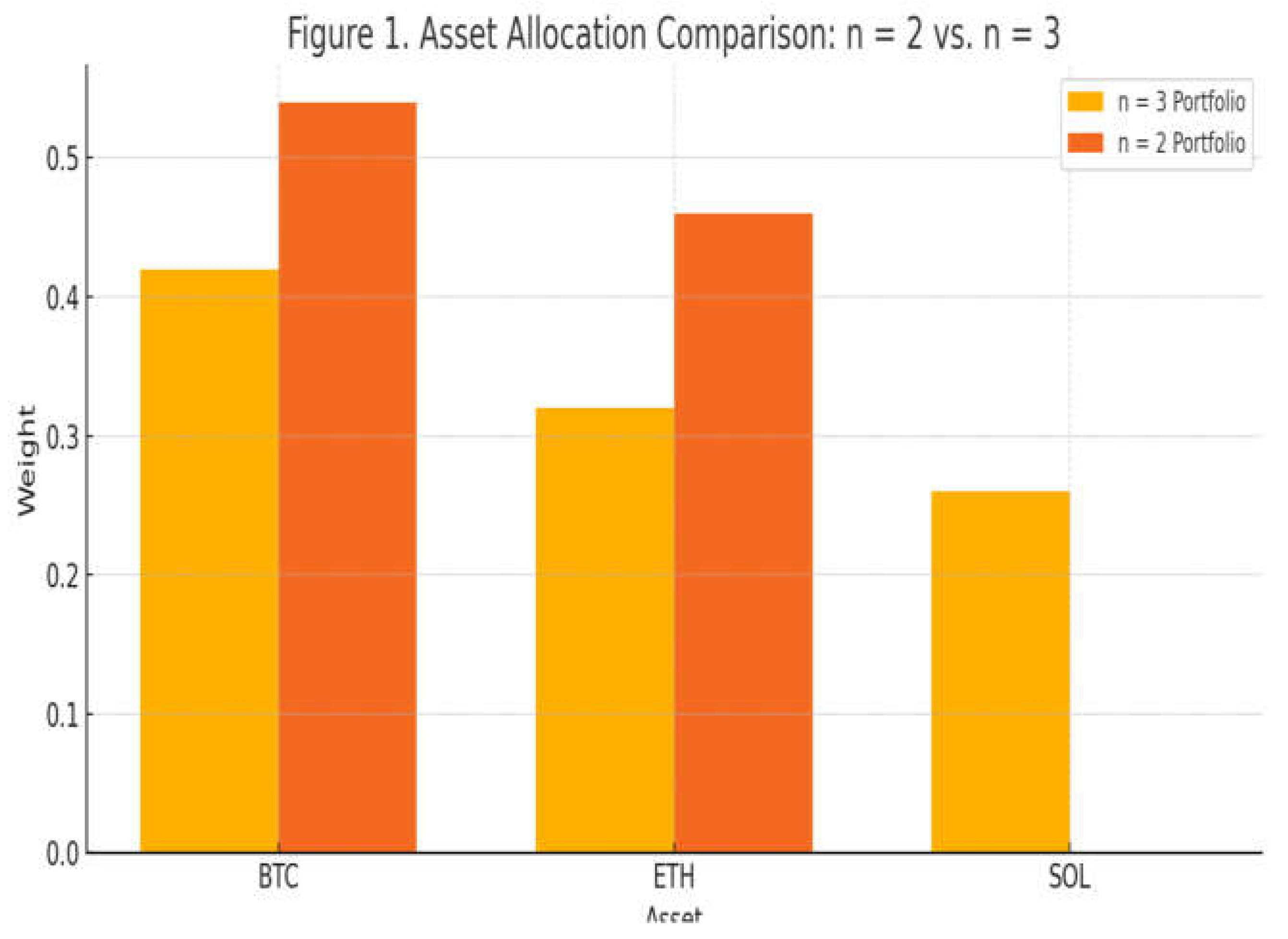
Figure 2.
Asset Allocation Based on Maximum Weighted Shannon Entropy Model.
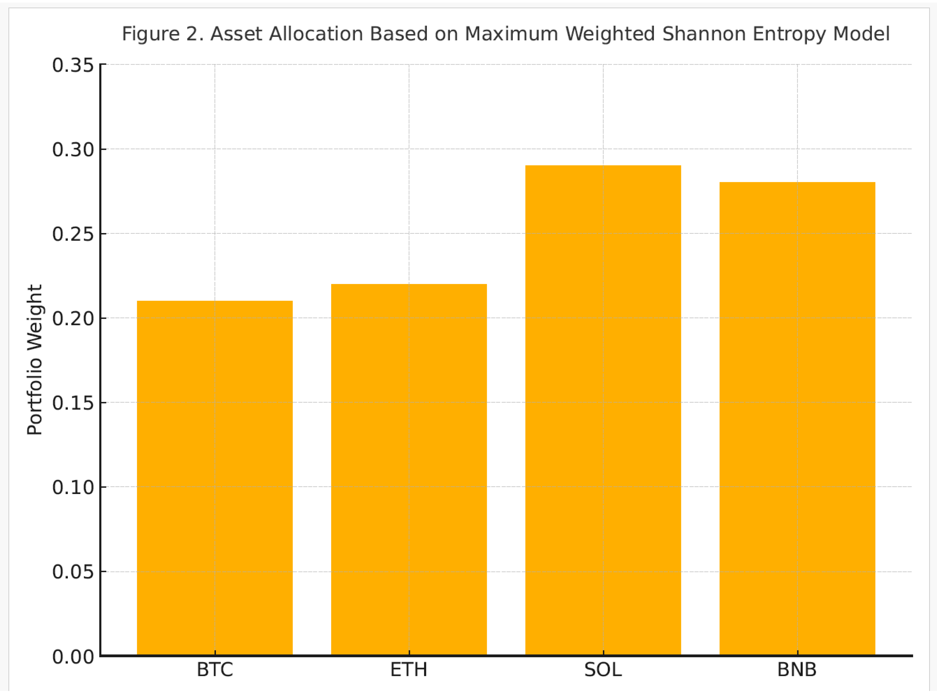

Table 1.
Portfolio Weights and Variance.
| Portfolio | Asset | Weight | Variance |
|---|---|---|---|
| n=2 | Bitcoin (BTC | 0.540 | 0.2916 |
| n=2 | Ethereum (ETH) | 0.460 | 0.2116 |
| n=3 | Bitcoin (BTC) | 0.420 | 0.1764 |
| n=3 | Ethereum (ETH) | 0.320 | 0.1024 |
| n=3 | Solana (SOL) | 0.260 | 0.0676 |
Disclaimer/Publisher’s Note: The statements, opinions and data contained in all publications are solely those of the individual author(s) and contributor(s) and not of MDPI and/or the editor(s). MDPI and/or the editor(s) disclaim responsibility for any injury to people or property resulting from any ideas, methods, instructions or products referred to in the content. |
© 2025 by the authors. Licensee MDPI, Basel, Switzerland. This article is an open access article distributed under the terms and conditions of the Creative Commons Attribution (CC BY) license (http://creativecommons.org/licenses/by/4.0/).
Copyright: This open access article is published under a Creative Commons CC BY 4.0 license, which permit the free download, distribution, and reuse, provided that the author and preprint are cited in any reuse.


