
Submitted:
14 April 2025
Posted:
14 April 2025
You are already at the latest version
Abstract
This research addresses the challenge of bias in Remotely Sensed Rainfall (RSR) datasets used for hydrological planning in Uganda’s data-scarce, ungauged catchments. Four bias correction methods; Quantile Mapping (QM), Linear Transformation (LT), Delta Multiplicative (DM), and Polynomial Regression (PR), were evaluated using daily rainfall data from four gauged stations (Gulu, Soroti, Jinja, Mbarara). QM consistently outperformed other methods across statistical metrics (e.g., for National Oceanic and Atmospheric Administration Climate Prediction Center (NOAA_CPC) RSR data at Gulu, Root Mean Square Error (RMSE) was reduced from 29.20 mm to 19.00 mm, Mean Absolute Error (MAE) reduced from 22.44 mm to 12.84 mm, and Percent Bias (PBIAS) reduced from -19.23% to 1.05%, and goodness-of-fit tests (KS = 0.03, p = 1.00), while PR, though statistically strong, failed due to overfitting. A bias correction framework was developed for ungauged catchments, using predetermined bias factors derived from observed station data. Validation at Arua (tropical savannah) and Fort Portal (tropical monsoon) demonstrated significant improvements in RSR data when the bias correction framework was applied. At Arua, bias correction of Climate Hazards Group InfraRed Precipitation with Station data (CHIRPS) data reduced RMSE from 49.14 mm to 21.41 mm, MAE reduced from 45.74 mm to 17.38 mm, and PBIAS reduced from -59.83% to -8.18%, while at Fort Portal, bias correction of CHIRPS dataset reduced RMSE from 28.35 mm to 15.02 mm, MAE from 25.28 mm to 11.35 mm, and PBIAS from -46.2% to 4.74%. The research concludes that QM is the most effective method and that the framework is a tool for improving RSR data in ungauged catchments. Recommendations for future work includes machine learning integration and broader regional validation.
Keywords:
Quantile Mapping
; Linear Transformation
; Delta Multiplicative
; Polynomial Regression
; Remote Sensing Rainfall
; Climate Zone
; and Annual Maximum Series.
1. Introduction
Rainfall plays a critical role in water resource modeling, management, agricultural planning, and the design of hydrological infrastructure such as culverts, road side channels, drainage systems, and irrigation networks as noted by Kimani et al., [1] and other authors [2,3,4]. Reliable rainfall data are globally of critical importance for assessing water availability, predicting flood risks, and addressing the challenges posed by climate variability and change according to Katiraie [4] and Maheswaran [5]. In regions with robust observational networks, ground-based rain gauges provide accurate and reliable rainfall measurements. However, according to Nkunzimana et al., [6] and other authors [7,8], in some African regions with sparse and unevenly distributed gauge networks such as Uganda, there are often significant uncertainties in rainfall estimates.
Remotely sensed rainfall (RSR) products offer a promising alternative, providing spatially continuous and near-real-time precipitation estimates as noted by Kimani et al., [1] and Mekonnen et al., [9]. Despite their potential, RSR products are not without flaws. Mekonnen et at., note that biases stemming from sensor calibration, retrieval algorithms, and the complexities of converting satellite signals into accurate rainfall rates limit their reliability [9]. Correcting these biases is essential before RSR data can be confidently applied to hydrological infrastructure design, especially in ungauged catchments where traditional gauge data are scarce or absent.
In recent years, flood-related disasters have caused widespread economic damage, infrastructure destruction, population displacement, and, in extreme cases, loss of life. In Uganda, Onyutha [10] and Ngoma et al., [11] in their research have reported the severe impacts of such flood events, while other researchers like Li et al., [12] predict that flood frequency and intensity will continue to rise. The approaches to design and build resilient hydrological infrastructure such as culverts, drainage channels, and bridges, particularly in ungauged catchments need to be explored more. At least it is among those strategies to minimize disruptions to economic development as floods grow more frequent and severe due to climate change and other factors. A key parameter in the design process is the design discharge, often derived from Intensity-Duration-Frequency (IDF) curves according to Andre et al., [13]. These curves relate rainfall duration and intensity to specific return periods, enabling engineers to design infrastructure capable of withstanding floods of a given magnitude as suggested by Galiatsatou [13] and others [14,15,16]. Subramanya [17] notes that constructing IDF curves requires an Annual Maximum Series (AMS), a record of the highest daily rainfall values for each year over an extended period, ideally spanning at least 25 years for hydrological purposes. AMS is a key component of extreme value analysis and plays a critical role in hydrological infrastructure design, including flood control structures, bridges, and drainage systems according to Gupta [18]. In data-scarce regions like Uganda, where rainfall monitoring stations are sparse or nonexistent, analyzing the applicability of the AMS of RSR data becomes essential. Therefore, the inherent biases in RSR products must be assessed and corrected according to Gumindoga et al., [19] and Mekonnen et al., [9] to ensure their suitability for estimation of design discharge.
Previous studies have explored the performance of RSR products in Uganda. For instance, Okirya and Du Plessis [3] evaluated the AMS of seven RSR products across different climate zones. They identified top performers like Global Precipitation Climatology Center (GPCC) (at Gulu, Jinja, and Soroti stations) and National Oceanic and Atmospheric Administration Climate Prediction Center (NOAA_CPC) (at Mbarara station) based on statistical metrics and goodness-of-fit performance tests. While their work highlighted variations in RSR performance tied to product type and location, it did not address the correction of inherent biases. Similarly, Onyutha [20] used AMS from observed data to evaluate Coordinated Regional Climate Downscaling Experiment (CORDEX) Regional Climate Models (RCM) simulations of extreme rainfall in East Africa, constructing IDF curves using data for the period 1961–1990 for the Lake Victoria Basin. However, the focus of his study was to evaluate the performance of CORDEX Africa RCM, driven by Coupled Model Inter-comparison Project Phase 5 (CMIP5) General Circulation Models (GCMs), in reproducing Extreme Rainfall Indices (ERIs), and not bias correction. Other studies in Uganda and East Africa by Macharia [7], and others [21,22], have evaluated RSR products, with Climate Hazards Group InfraRed Precipitation with Station data (CHIRPS) being the most extensively studied. Further research is still needed to explore and correct the biases in the AMS of RSR products. The biases need to be systematically evaluated and corrected to ensure the accuracy and reliability of RSR products for hydrological applications in ungauged or sparsely gauged catchments.
Previous studies have investigated various Bias Correction Techniques (BCTs) to address the challenge of inherent biases in RSR products. For instance, Ajaaj et al., [23] evaluated five bias BCTs to adjust GPCC rainfall data in Iraq, finding that Quantile Mapping and mean bias removal methods outperformed others, with performance varying by season and climate zone. Similarly, Ouatiki et al., [24] evaluated five bias correction techniques (BCTs) across eight satellite-based rainfall datasets in Morocco. The study revealed improvements in bias correction for the RSR dataset using methods such as Random Forest, with effectiveness varying based on local climatology.
In Uganda, Nakkazi et al., [8] used Local Intensity Scaling (LOCI) and Linear Scaling (LS) to correct precipitation data for the Soil and Water Assessment Tool (SWAT) model in the Manafwa catchment. They found the LS method failing to capture extreme events, while LOCI only partially addressed heavy rainfall. Their study, highlighted the need for further research into extreme value correction. These studies demonstrate that while bias correction is effective in regions with dense gauge networks, its application in ungauged or poorly gauged areas remains challenging. Uganda’s diverse climate, from western highlands to eastern lowlands, further complicates matters, as correction parameters may not be transferable across regions with different climatology.
Emerging research has turned to machine learning (ML) approaches for bias correction, with studies like those by Nguyen et al., [25] and others [26,27,28,29,30] showing improved RSR accuracy. However, ML methods often rely on historical gauge rainfall data, incur high computational costs, and lack transferability, posing obstacles for data-scarce regions like Uganda. Addressing these challenges requires a flexible, locally tailored bias correction framework that can enhance RSR data for hydrological infrastructure design in ungauged catchments. Several studies, including those by Dao et al., [26] and others [27,28,29], have applied ML-based bias correction frameworks to RSR datasets and registered promising results. For example, Chen et al., [28], developed a deep Convolutional Neural Network (CNN) framework and successfully reduced biases in the NOAA Climate Prediction Center Morphing Technique (CMORPH) rainfall product. While ML approaches yield promising results, they also introduce uncertainties related to assumptions of regional homogeneity and transferability of bias correction parameters across different climate zones. In Uganda, Nakkazi et al., [8] applied a bias correction framework based on the Soil and Water Assessment Tool (SWAT) model to validate bias-corrected RSR datasets in Manafwa catchment. The SWAT model was calibrated using the bias corrected RSR datasets (Climate Forecasting System Reanalysis (CFSR), MERRA-2, and TRMM3B42) as input rainfall data. The effectiveness of RSR data bias correction was assessed by how well SWAT-simulated streamflow matched observed streamflow, using performance metrics such as Nash-Sutcliffe Efficiency (NSE), PBIAS, and RMSE. The bias correction framework by Nakkazi et al., [8] was applied in a small catchment and considered a monthly temporal scale and not daily scale, which is relevant to hydrological infrastructure designs and planning.
Reliable rainfall data underpin effective hydrological infrastructure design, flood risk management, water supply, and agricultural planning. In Uganda, where many catchments lack sufficient ground-based observations, refining RSR data through bias correction offers viable alternatives to observed measurements. This research aims to bridge existing gaps by evaluating conventional bias correction methods in gauged catchments, adapting the best-performing approaches for ungauged areas, and providing actionable insights for policymakers and engineers in Uganda and similar regions.
The research evaluates four conventional bias correction methods; Linear Transformation (LT), Quantile Mapping (QM), Delta Multiplicative (DM), and Polynomial Regression (PR), in gauged catchments using data from four stations. Performance is assessed through metrics Root Mean Square Error (RMSE), Mean Absolute Error (MAE), Percent Bias (PBIAS), and Nash-Sutcliffe Efficiency (NSE)), visual comparisons from rainfall time series plots, and goodness-of-fit tests (Kolmogorov-Smirnov (KS) test statistics and p-values). Based on these results, a flexible framework is developed to correct RSR data in ungauged catchments by estimating observed rainfall parameters using predetermined correction factors. The framework’s reliability is then validated with independent data from two additional gauged stations, ensuring its robustness for supporting estimation of design discharge for hydrological infrastructure design.
1.1. Objectives
The research’s main and specific objectives are outlined below.
1.1.1. Main Objective
The primary goal is to evaluate and compare bias correction methods, then develop and validate a framework for correcting remotely sensed rainfall data in ungauged catchments in Uganda.
1.1.2. Specific Objectives
The specific objectives are:
- To evaluate and compare the performance of four bias correction methods; Linear Transformation, Quantile Mapping, Delta Multiplicative, and Polynomial Regression, in gauged catchments.
- To develop a bias correction framework for ungauged catchments by adapting the best-performing methods from gauged catchments.
- To validate the framework using an independent dataset from selected gauged stations.
1.2. Research Questions
The research addresses the following questions:
- How do bias correction methods compare in their ability to adjust RSR data in gauged catchments in Uganda?
- How can the optimal bias correction methods from gauged catchments be adapted for use in ungauged catchments?
- How effective is the bias correction framework in ungauged catchments in Uganda?
2. Materials and Methods
2.1. Description of the Study Area
The study area is Uganda which is located in the East African region (Figure 1). The country is distinguished by its diverse climatic zones and varied topography. According to the Köppen–Geiger global climate classification raster data file by Beck et al. [31] for 1991–2020 period, Uganda features nine distinct climatic zones. The country predominantly experiences a bimodal rainfall regime, characterized by two rainy seasons—March to May and September to November—though regional variations exist, as noted by Ngoma et al., [11] and Jury [32]. According to Ngoma et al., [11], the annual rainfall across Uganda ranges widely from 750 to 2,500 mm, with mean annual precipitation typically falling between 800 and 1,500 mm. Higher rainfall is observed in the highland areas, while semi-arid regions in the east receive lower amounts. Temperatures in Uganda remain relatively moderate, with average annual values ranging from 20°C to 27°C, shaped by altitude and local weather patterns [3,8]. The country’s terrain is equally diverse, encompassing towering mountains, and low-lying plains. Notable peaks include the Rwenzori Mountains in the southwest, rising to about 5,109 meters, and Mount Elgon in the east, reaching about 4,321 meters as noted by Ngoma et al., [2,11]. These climatic and topographical variations make Uganda an ideal region for studying RSR bias correction in both gauged and ungauged catchments.
2.2. Research Data
This research utilized AMS of observed rainfall and RSR datasets covering the period of 1991–2020. The observed rainfall data was obtained from 6 gauging stations across Uganda (Figure 1) and seven different RSR datasets. The AMS comprises the highest observed daily rainfall total (recorded from 0900 hours to 0859 hours) for each year over a 30-year period, as described by Subramanya [17] and Maity [33].
2.2.1. Observed Rainfall Data
The observed daily rainfall data from six stations; Gulu, Soroti, Jinja, Mbarara, Arua, and Fort Portal, was obtained from the Uganda National Meteorological Authority (UNMA). The dataset spans a 30-year period, from January 1, 1991, to December 31, 2020. Before being used in the analysis, the data underwent standard quality checks, as detailed in subsequent sections.
2.2.2. Remotely Sensed Rainfall (RSR) Data
In this research, RSR data products, widely recognized in the literature as gridded precipitation products, refers to three categories of remotely sensed rainfall data: (a) gauge-only derived products, (b) products combining satellite and gauge data, and (c) numerical weather prediction products. The gauge-only derived product comprised the Global Precipitation Climatology Centre (GPCC), operated by the Deutscher Wetterdienst (DWD) under the World Meteorological Organization (WMO), offers gridded precipitation datasets from quality-controlled station data as noted by S. E. Nicholson and D. A. Klotter [34]. The Satellite-gauge products which integrate gauge and satellite data through various bias corrections comprised: (a) the Precipitation Estimation from Remotely Sensed Information using Artificial Neural Networks-Climate Data Record (PERSIANN_CDR) from the University of California, Irvine, which uses neural networks for global daily rainfall estimates since 1983 according to Omonge et al., [9] and others [22,35]; (b) the Climate Hazards Group InfraRed Precipitation with Station data (CHIRPS) from the University of California, Santa Barbara, and the United States Geological Survey (USGS), integrating satellite and in-situ data for high-resolution rainfall monitoring [7,9,35,36]; and (c) the Climate Prediction Center (CPC) Unified Gauge-Based Analysis of Global Daily Precipitation from the National Oceanic and Atmospheric Administration (NOAA_CPC), which provides gauge-based global rainfall estimates supporting climate studies [3]. The numerical weather prediction products derived from atmospheric models (the Reanalysis products) included; (a) the Modern-Era Retrospective Analysis for Research and Applications, Version 2 (MERRA-2) from the National Aeronautics and Space Administration (NASA), a reanalysis dataset incorporating advanced assimilation techniques since 1980 [8,34]; (b) the European Centre for Medium-Range Weather Forecasts (ECMWF) Reanalysis v5 (ERA5) and (c) ECMWF Reanalysis v5 for Agriculture (ERA5_AG) datasets, providing daily and hourly global climate estimates from 1940 onward with a focus on land surface applications [9].
2.3. Data Preprocessing
Okirya and Du Plessis [3] provide a detailed description of data preprocessing for rainfall data from four stations; Gulu, Soroti, Jinja, and Mbarara. This research utilizes the same data from the same stations, along with additional data from the Arua and Fort Portal stations. The preprocessing steps outlined in the study by Okirya and Du Plessis [3] have been applied to rainfall datasets obtained for the Arua and Fort Portal stations. The preprocessing steps among other included outlier detection using box plots and time series plots, followed by rainfall gap-filling techniques for missing values.
2.3.1. Data Quality Checks
Two key rainfall data quality issues were addressed in this research: (a) data completeness (gaps in raw rainfall data), and (b) the presence of outliers.
To assess data completeness, the rainfall dataset was organized in an Excel worksheet, where dates and corresponding daily rainfall values were arranged in separate columns; one column for the date and another for rainfall measurements. A separate reference date column was introduced, containing continuous dates from January 1, 1991, to December 31, 2020 for purposes of comparison or matching dates. This approach allowed for a straightforward comparison between the expected date sequence and the dates accompanying the actual rainfall measurements, thereby revealing any mismatches that indicated data gaps. Once gaps were detected, appropriate gap-filling techniques were applied to maintain continuity in the time series.
The outlier detection was conducted using both visual and statistical methods. Time series plots were used to visualize extreme values that deviated significantly from the general trend. Graphical tools such as box plots were also employed to identify isolated rainfall values that occurred out of line with the majority of observations. Following the Interquartile Range (IQR) approach, rainfall values that fell outside the range Q1 - 1.5 IQR and (Q3 + 1.5 IQR) were classified as outliers. The IQR method, defined as the difference between the first (25th percentile) and third (75th percentile) quartiles, is widely used for detecting extreme values as suggested by Maity [33] and others [37,38]. However, as demonstrated by Okirya and Du Plessis [3], the IQR method tends to identify high extreme values as outliers. Consequently, it was applied with additional verification of extreme values using time series plots.
2.3.2. Gap Filling of Rainfall Data and Treatment of Outliers
For the observed rainfall data, gaps with missing rainfall values lasting between one to four days were filled using the linear interpolation method. For longer gaps, extending up to 30 days, the long-term mean approach was applied. The long-term mean method is simple, quick, and preserves historical trends. The method is mostly applicable for datasets with less than 10% of the missing values over the period under consideration as noted by Chinasho et al., [39]. Unlike Chinasho et al., ., [39] and Phan et al., [39,40] who used neighboring station averages to fill gaps in rainfall data at the station of interest, this research applied the long-term mean of historical rainfall values from the same station. Although the long-term mean method preserves historical trends, it may not account for climate-induced variability in rainfall data which deviates from historical trends. Consequently, any extreme weather patterns occurring within the missing period may not be accurately represented by a long-term mean value. Nevertheless, this approach remains an effective strategy for ensuring data completeness in rainfall time series analysis. The long-term mean is estimated using Equation 1:
where: d is the long-term mean rainfall estimate, Xd represents the observed rainfall on the same calendar day (d) in different years, and n is the number of rainfall data available.
For the RSR data (specifically NOAA_CPC), rainfall data gaps of one to four days were similarly addressed using linear interpolation. However, for longer gaps of up to 31 days, particularly in the PERSIANN_CDR dataset, missing rainfall values were filled using station regression coefficients. These coefficients were derived from Double Mass Curve plots, comparing the cumulative rainfall of PERSIANN_CDR with NOAA_CPC datasets (both satellite-gauge derived products). The remaining RSR datasets (CHIRPS, GPCC, MERRA2, ERA5, and ERA5-AG) showed no gaps in their rainfall time series after undergoing data quality checks. The relationship used for estimating missing values is expressed shown in Equation 2.
where: y represents the missing PERSIANN_CDR rainfall value, m the station regression coefficient, and x the corresponding NOAA_CPC RSR dataset values.
Applying this regression equation (2) to the PERSIANN RSR data at Arua and Fort Portal stations individually yielded the specific equations shown in Table 1.
The outliers were replaced with the corresponding 95th percentile rainfall value for the respective years.
2.4. Evaluating and Comparing Bias Correction Methods in Gauged Catchments
The evaluation process involved applying each bias correction method to the RSR data and assessing the bias-corrected outputs against observed rainfall records using both statistical metrics, goodness-of-fit test, and graphical visualizations.
2.4.1. Bias Correction Methods
Each bias correction method was applied to all seven RSR dataset products from four gauged stations, with validation extended to two additional stations. Below, the methods are described, highlighting their applicability.
The LT method corrects biases by aligning the mean and variance of the RSR dataset with those of the observed rainfall data, as described by Gado et al., [41]. and Ajaaj et al., [23]. The adjustment follows Equation 3.
where: Radj is the bias corrected RSR data, RRSR is the original (uncorrected) RSR data, σobs and μobs are the standard deviations and the mean of the observed data, while μRSR and σRSR are the mean and standard deviation of the original (uncorrected) RSR data.
The LT method is simple and computationally efficient, making it a widely used method in bias correction. However, it only adjusts the first two statistical moments (mean and variance), without addressing higher-order moments such as skewness or kurtosis. This means that if the bias between observed and RSR data is non-linear, particularly at the extremes, the method may not adequately capture these differences as noted by Ajaaj et al., [23] and Ehret et al.,[42].
The QM method is one of the most popular and widely used bias correction techniques, as noted by several authors including Enayati et al., and others [4,12,43]. The QM approach corrects biases by matching the Cumulative Distribution Functions (CDFs) of the observed rainfall and RSR datasets. The approach follows Equation 4, as described by Xiaomeng et al., and others., [12,44,45].
where FRSR (RRSR) is the Cumulative Distribution Function (CDF) of the RSR data evaluated at the RSR value, and is the inverse CDF (or the quantile function) of the observed data [24].
The QM method is generally effective because it adjusts the entire distribution, preserving extreme rainfall values and improving accuracy across different rainfall intensities as noted by Ehret et al., [42]. However, QM requires a sufficiently long time series to estimate quantiles accurately, and its effectiveness may be limited in datasets with short records or missing values as noted in a study by Koutsouris et al., [46].
The DM method as defined in Equation 5, scales the RSR dataset using the ratio of the observed mean to the uncorrected RSR mean as suggested by Nakkazi [8] and others [24,41,47]
where Radj is the adjusted (bias corrected) RSR data and RRSR is the original (uncorrected) RSR data; while and denote the means of observed and RSR data, respectively.
The DM approach, like LT, is simple and computationally efficient [23]. The method preserves the original shape of the RSR distribution by applying a uniform scaling factor across all values. However, DM only corrects the mean and does not adjust the variance or other statistical properties of the dataset [41,42]. As a result, if biases vary across different rainfall magnitudes, this method may be insufficient in capturing variability and extreme events as noted by Ehret et al., [42].
The PR method extends linear correction techniques by introducing a non-linear relationship between the RSR and observed datasets. A commonly used form is the quadratic (second-degree) polynomial model, as presented in Bluman and other publications [33,48,49]. The method follows Equation 6.
where Radj is the adjusted (bias corrected) RSR data and RRSR is the original (uncorrected) RSR data; while a, b, and c are coefficients determined through regression analysis.
The PR is particularly beneficial when the bias between observed and RSR data is non-linear, as it can capture curved relationships that linear methods fail to model. However, the approach comes with several limitations. According to Ajaaj et al. [23], polynomial models are prone to overfitting, especially when higher-degree polynomials are used with limited data. Additionally, polynomial regression models can behave erratically when extrapolating beyond the calibration range and are sensitive to outliers, which may distort the fitted curve.
2.4.2. Statistical Performance Metrics
The performance of each of the bias correction methods were quantitatively assessed using several statistical metrics including RMSE, MAE, PBIAS, NSE, and goodness-of-fit tests (KS statistic and p-value). The methods are very popular and have been widely used in a number of studies by several authors including Kimani et at., and others [1,36,44,50,51], to assess the performance of bias correction methods. The equations for these statistical metrics are presented in Table 2 shown.
In hydrological applications, PBIAS values of less than ±10% are considered very good performance, ±10% to ±15% indicate good performance, while ±15% to ±25% indicate fair performance [8,50]. For the NSE metric, a value of 1 indicates a perfect match between the bias-corrected data and the observed values while negative values imply poor performance as noted by Diem et al., [52]. The NSE method is usually used for models that simulates the hydrological variables by measuring the model efficiency in terms of relative variance in simulation error compared to variance of observed variable [33].
2.4.3. Goodness-of-Fit Tests
Among the most widely used goodness-of-fit tests for comparing Probability Density Functions (PDFs) and CDFs are: (i) the Chi-Squared Test and (ii) the Kolmogorov–Smirnov (KS) Test. As noted by Karamouz et al., [53], the Chi-Squared Test is more effective when the sample size is large, as it relies on frequency distributions that require a sufficient number of observations for accurate assessment. However, in cases where the sample size is small, such as in this research (30 data entries), the KS Test is more appropriate. The KS test is a non-parametric test, meaning it does not assume any specific distribution for the dataset. It measures the maximum difference between the empirical cumulative distribution functions (CDFs) of the observed data and the bias-corrected data, providing an indication of how well the corrected data aligns with the original observations [33]. The test statistic (KS) is mathematically defined in Equation 7.
where Fobs,n(x) and Fadj,n(x) are the empirical CDFs of the observed and the RSR bias-corrected data, respectively, and Max indicates the maximum absolute difference across all values. A smaller Dn value (KS statistics) and higher p-value greater than 5% significance level indicates a closer match between the two empirical CDFs [33].
2.4.4. Visual Assessment
The visual assessment of bias correction methods uses the time series plots and PDF/CDF curves to compare observed rainfall, uncorrected RSR data, and bias-corrected RSR datasets. These plots enable visual assessments on how well the bias corrected data reflects temporal patterns, yearly changes, and extreme events relative to actual observations, revealing any major deviations. The PDF comparison evaluates bias correction performance by showing how RSR data are distributed and how different the distribution is from that of observed rainfall data. A good method aligns the RSR corrected PDF’s shape, spread, and peak with the observed PDF, while deviations, shifted peaks or distorted spread, indicate under- or over-correction, potentially skewing variability or extremes. The CDF comparison examines the cumulative probability of rainfall amounts, assessing how well the corrected data matches the observed frequency distribution. An effective method keeps the corrected CDF close to the observed one, whereas shifts or slope differences suggest issues like missing extremes or misrepresented frequencies.
2.5. Development of RSR Bias Correction Framework for Ungauged Catchments
This research proposes a flexible regionalized framework to bias-correct RSR data in ungauged catchments, using bias correction factors derived from gauged catchments, as well as predetermined bias correction factors. The predetermined bias correction factors represent the highest or lowest systematic biases (consistent overestimation or underestimation of rainfall values compared to observed data) identified across the four stations. The regionalization approach involves transferring bias correction parameters (such as mean and standard deviation) from the nearest gauged station within the same climatic zone as the ungauged catchment. This approach assumes that catchments within the same climatic zone exhibit similar bias characteristics as suggested by Yang et al., [54,55,56].
For cases where an ungauged catchment is located in a climatic zone with no nearby station or lacks historical observed data, the proposed framework will apply predetermined bias correction factors to adjust the original RSR data. These correction factors are based on the assumption that RSR biases can be systematic [1,4], or random, yet consistent within a given climatic zone. While the magnitude of biases may vary, the direction (either overestimation or underestimation) is expected to remain consistent across locations and climate zones. If the RSR data lacks consistent biases or displays mixed errors (both overestimation and underestimation across stations), it is rejected, and the process is terminated. For datasets that pass this screening by exhibiting consistent errors, the framework standardizes the RSR data into Z-scores to normalize it, enabling the continuation of the bias correction process.
The RSR bias correction framework adapts the best-performing bias correction methods tested in gauged catchments considering two scenarios:
- In ungauged catchments located near a gauged station within the same climatic zone, LT, QM, DM, and PR methods are applied using regionalized parameters (mean and standard deviation) derived from the closest gauged station. The predetermined bias correction factors could also be applied using the LT and DM methods.
- If the ungauged catchment is in a climate zone with no observed data, the framework relies on predetermined bias correction factors (mean and standard deviation) de-rived from the four gauging stations to bias correct the RSR datasets.
Each RSR product’s bias is examined across the four reference gauged stations of Gulu, Soroti, Jinja, and Mbarara. If systematic errors (consistently overestimated or underestimated rainfall values) are identified across the four stations, the highest or lowest biases (predetermined bias correction factors) from these stations will be applied to the ungauged catchments. The RSR datasets with inconsistent bias patterns (overestimated and underestimated for the same product across gauging stations) will be excluded from further analysis.
The bias correction framework is then implemented following the bias correction expressions shown in Equations 3 to 6. To validate the framework, the optimal bias correction methods identified in the four gauged catchments are adopted for implementation at the two additional catchments for further assessment. The performance of the bias correction methods are then assessed on how well the corrected RSR datasets using metrics like RMSE, MAE, PBIAS, NSE, and the K-S test. In addition to these metrics, the visual assessments including the use of time series plots, the PDF and CDF plots are deployed to compare how the bias corrected RSR datasets align with observed rainfall data.
2.5.1. Biases in RSR Data Products
Biases in each RSR dataset are estimated as the difference between observed rainfall and RSR data at each station, following the formula in Equation 8 [23,24].
The over- or under-estimation in biases of the RSR datasets across the four gauged stations are identified by comparing the bias values at each of the stations. If a RSR dataset consistently overestimates or underestimates rainfall across multiple stations, it indicates a systematic bias that can be corrected using the proposed framework.
2.5.2. Regionalized Parameters for Bias Correction
The regionalized parameters apply when an ungauged catchment lies in a climatic zone with a nearby gauged station with observed rainfall data. Here, observed data from similar zones provide means and standard deviations, which are transferred to the ungauged site. In climate zones lacking gauging stations, these parameters (mean and standard deviations) are estimated from predetermined bias correction factors using Equations 9 and 10, for mean and standard deviation, respectively. The predetermined bias correction factors are applied to parameters which are used in the LT and DM bias correction methods.
where μobs is estimated mean of what would have been observed data at the ungauged catchment, μRSR is the mean of RSR data at the ungauged catchment, and Δμ is the predetermined bias correction factor for the mean value.
For the standard deviation:
where σobs is estimated standard deviation of what would have been observed data at the ungauged catchment, σRSR is the standard deviation of RSR data at the ungauged catchment, and Δσ is the predetermined bias correction factor.
3. Results
3.1. Data Quality Control and Preprocessing Results
The data quality issues and preprocessing results for the observed and RSR rainfall datasets at Gulu, Soroti, Jinja, and Mbarara stations are presented in the publication by Okirya and Du Plessis for reference [3].
3.1.1. Identified Gaps in Rainfall Data
At Arua station, visual inspection and checking mismatches in dates revealed some gaps in the observed rainfall data. Particularly, the entire month of November 1993 and the entire month of October 1998 had missing data, along with a missing value on February 29, 2020. Overall, the percentage of missing rainfall data at the Arua station was approximately 0.557% for observed station data. For the RSR datasets at the Arua station, the NOAA_CPC dataset exhibited isolated one-day gaps on several dates, amounting to a missing rainfall data percentage of about 0.046%. In contrast, the PERSIANN_CDR product showed a larger gap, with the entire month of February 1992 (29 days) missing, along with other gaps ranging from 1 to 15 days, resulting in an overall missing percentage of 0.949%. The rest of the RSR products at this station did not have missing rainfall data values.
At the Fort Portal station, the observed rainfall data exhibited relatively small gaps, with one-day missing entries recorded on four separate dates, resulting in a missing rainfall data percentage of 0.037%. The NOAA_CPC RSR product at Fort Portal had a slightly higher missing rainfall data percentage of 0.046%, while the PERSIANN-CDR product displayed even a larger gap, with a missing rainfall data percentage of 0.949%.
Figure 2 shows the identified gaps in both the observed and RSR datasets at the Fort Portal and Arua stations.
3.1.2. Outlier Detection and Removal
The Interquartile Range (IQR) box plots (Figure 3) identified numerous rainfall values as potential outliers. However, time series plots were used to distinguish genuine extreme rainfall events from outlier data points. Figure 3 and Figure 4 show the outliers identified at the Fort Portal and Arua rainfall stations, respectively. At the Fort Portal station, outliers were detected only in the observed data, with extreme values of 337 mm on September 28, 2006, and 183.3 mm on November 12, 1994. These were replaced by the 95th percentile values of 20.34 mm and 25.01 mm, respectively, computed specifically for the respective years.
At the Arua station, for the GPCC product, extreme outliers of 264.74 mm on October 17, 1992, and 209.39 mm on August 08, 2013, were identified. For each of these years, the 95th percentile of the rainfall data were computed as 34.36 mm and 34.56 mm, respectively, and these values were used to replace the outliers. Similarly, in the MERRA2 dataset at the Arua station, outliers of 209.13 mm on August 22, 2017, 226.84 mm on March 10, 2018, and 205.74 mm on December 09, 2020, were replaced with the corresponding 95th percentile values of 29.38 mm, 30.34 mm, and 24.33 mm, respectively.
3.2. Evaluation and Comparison of Bias Correction Methods in Gauged Catchments
3.2.1. Visual Comparison of Time Series Plot Results
The time series plots presented in Figure 5, Figure 6, Figure 7 and Figure 8 (Gulu (Figure 5), Soroti (Figure 6), Jinja (Figure 7), and Mbarara (Figure 8)) provide a visual comparison of the performance of four bias correction methods, alongside the original (uncorrected) RSR data. The observed rainfall, represented by a black line, serves as the benchmark for assessing each method’s ability to align RSR data patterns, capture inter-annual variability, and accurately reflect extreme rainfall events. From the time series plots two main observations are drawn. First, among the evaluated methods, Quantile Mapping (depicted in green) consistently emerges as the top performer across all stations and RSR datasets. It closely mirrors the observed rainfall peaks and troughs, demonstrating better alignment. Following the Quantile Mapping method, both Linear Transformation (orange) and Delta Multiplicative (red) methods show moderate improvements over the uncorrected data. They align better with observed trends and successfully adjust the RSR data to preserve inter-annual variability and capture extreme rainfall peaks to some extent. However, they occasionally underestimate peaks, as seen with the CHIRPS dataset at the Gulu station, where these methods fail to reach the observed maximum rainfall values. Second, the Polynomial Regression method (purple) performs poorly across all four stations, exhibiting significant limitations. At Gulu, it fails to capture inter-annual variabilities in CHIRPS, GPCC, PERSIANN, and ERA5 datasets, producing overly smoothed trends. Similarly, at Jinja, it misaligns with NOAA_CPC and ERA5 data; at Mbarara, it underperforms with ERA5_AG and ERA5; and at Soroti, it is misaligned with MERRA2 and PERSIANN. This method consistently fails to track extreme rainfall events and shows a clear misalignment with observed patterns, rendering it unsuitable for effective bias correction applications.
Across all stations and datasets, the original (uncorrected) RSR data, represented by a blue line, consistently underestimates observed rainfall. This underestimation is particularly pronounced in certain cases, such as with CHIRPS, ERA5, PERSIANN, MERRA2, and ERA5_AG datasets at Jinja and Soroti stations, where the gap between observed and uncorrected data is substantial. Similarly, at Gulu and Mbarara stations, the underestimation is evident with CHIRPS, ERA5, PERSIANN, and ERA5_AG.
3.2.2. Results of Statistical Performance Metrics
The statistical performance test results for the RSR datasets across the four stations are presented in Table 3 (Gulu and Soroti stations) and Table 4 (Jinja and Mbarara stations).
The statistical performance results reveal that the original (uncorrected) Remote Sensing Rainfall (RSR) datasets consistently exhibit high RMSE, MAE, and PBIAS values, coupled with higher negative NSE values, signifying severe underestimation of observed rainfall. All the bias correction methods, Linear Transformation, Quantile Mapping, Delta Multiplicative, and Polynomial Regression, generally reduce RMSE, MAE, and absolute PBIAS compared to the original datasets, though their success varies.
Among the four bias correction methods evaluated, Quantile Mapping (QM) emerged as the most effective, particularly at the Gulu and Jinja stations. At Gulu, applying QM to the NOAA_CPC dataset significantly improved performance, reducing the RMSE from 29.20 mm to 19.00 mm (a 35% improvement), MAE from 22.44 mm to 12.84 mm (a 43% improvement), and PBIAS from -19.23% to 1.05% (a 95% improvement). Similarly, at Jinja, QM applied to the GPCC dataset achieved an RMSE of 17.96 mm, down from 22.22 mm (a 19% improvement), MAE of 14.36 mm from 17.56 mm (an 18% improvement), and PBIAS of 1.25% from -14.64% (a 91% improvement).
The Linear Transformation (LT) method also delivered strong performance, particularly at the Mbarara station where it was applied to the GPCC dataset. The method reduced the RMSE from 22.62 mm to 20.66 mm (a 9% improvement), the MAE from 16.60 mm to 14.98 mm (a 10% improvement), and achieved a PBIAS of 0.00% from -5.93% (100% improvement). The Delta Multiplicative (DM) method, though generally exhibiting higher errors than QM and LT at most stations, proved particularly most effective at Soroti. Applied to the CHIRPS dataset, it significantly reduced the RMSE from 37.67 mm to 20.89 mm (a 45% improvement) and the MAE from 33.07 mm to 15.68 mm (a 53% improvement), while correcting the PBIAS from -45% to 0.00% (a 100% correction).
The Polynomial Regression (PR) method consistently recorded the lowest RMSE (ranging from 15.34 mm for NOAA_CPC at Mbarara to 16.75 mm for CHIRPS at Gulu) and MAE values (from 10.94 mm at Soroti to 13.06 mm at Gulu). It also yielded a PBIAS of 0.00% across all RSR datasets and achieved the highest Nash-Sutcliffe Efficiency (NSE) values, including 0.19 for NOAA_CPC and GPCC at Jinja and Mbarara, and 0.01 at Gulu. While these metrics initially suggest superior performance, further inspection reveals limitations. The analysis of time series plots (Figure 5, Figure 6, Figure 7 and Figure 8) and goodness-of-fit tests (KS statistics and p-values) indicates that PR tends to over fit the data, producing overly smoothed trends that fail to represent inter-annual variability and extreme rainfall events. This overfitting, despite strong statistical performance, compromises the method’s practical utility, rendering it less reliable for real-world hydrological applications.
3.2.3. Results Based on the Visualization of PDF and CDF Plots
Figure 9, Figure 10, Figure 11 and Figure 12 present Probability Density Functions (PDFs) and CDFs for observed rainfall, original (uncorrected) RSR data, and bias-corrected RSR datasets across four gauged stations: Gulu (Figure 9), Soroti (Figure 10), Jinja (Figure 11), and Mbarara (Figure 12).
Based on the shapes of the PDFs and CDFs, Quantile Mapping (green line) emerges as the standout bias correction method, outperforming others by closely mirroring the distribution of observed rainfall data (black dashed line). This near-perfect alignment is evident across multiple RSR datasets at all stations. For instance, at Gulu, the Quantile Mapping PDF and CDF align seamlessly with the observed data across the full range of rainfall values, accurately capturing the distribution’s peaks, spreads, and tails. Similarly, at Soroti and Jinja, this method consistently reflects the observed rainfall characteristics.
The Linear Transformation and Delta Multiplicative methods also demonstrate improvement over the original (uncorrected) RSR data, nonetheless, they fall short of Quantile Mapping’s performance. This is most apparent in their inability to accurately represent higher rainfall amounts, as seen in the flattened tails of their PDFs and the noticeable divergence of their CDFs from the observed data. For example, for NOAA_CPC, GPCC, and MERRA2 RSR data at Gulu station (Figure 9), both methods show a reduced capacity to match the observed distribution at higher rainfall thresholds compared to Quantile Mapping.
The PDF of all RSR data adjusted with the Polynomial bias correction method markedly deviates from the observed data’s distributional shape at all stations. The Polynomial method produces overly sharp peaks, a sign of overfitting, and poorly captures the spread or variance of the observed rainfall. Despite this, across all RSR datasets and stations, the Polynomial method aligns the central tendency (mean and median) of the adjusted data more closely with the observed data than the original, uncorrected RSR does. Furthermore, the Polynomial CDF diverges at the tails, either underestimating or overestimating extreme values (very low or very high rainfall), as indicated by its nearly vertical slopes across all adjusted RSR datasets and stations, highlighting its failure to represent the full range of rainfall variability.
Overall, the bias-corrected RSR data significantly outperforms nearly all original (uncorrected) RSR datasets. This improvement is particularly pronounced for the CHIRPS, ERA5, PERSIANN, ERA5_AG, and MERRA2 datasets across all stations as seen from Figures 9 – 12. However, an exception occurs with the GPCC data at the Gulu station, where the uncorrected data demonstrates relatively better performance.
3.2.4. Results Based on the Goodness-of-Fit Test (KS and p-Values)
Table 5 presents the goodness-of-fit test results, detailing the KS statistics and corresponding p-values for four bias correction methods, alongside the original (uncorrected) RSR data.
Among the bias correction methods, Quantile Mapping consistently delivered the best goodness-of-fit results, achieving KS statistics as low as 0.03 and p-values of 1.00 across all stations and datasets. This indicates an excellent distributional match between the RSR products and observed rainfall data. Linear Transformation also improves the fit over the original RSR data, with KS statistics typically ranging from 0.10 to 0.30 and p-values often between 0.39 and 1.00. For example, at Mbarara, the Linear Transformation method for the CHIRPS dataset achieves a KS statistic of 0.10 with a p-value of 1.00, indicating a near-perfect fit. The Delta Multiplicative method exhibits mixed results, with KS statistics varying widely from 0.10 (for ERA5_AG at Gulu) to 0.33 (for MERRA2 at Mbarara) and p-values ranging from 0.03 (for ERA5_AG at Jinja and Soroti) to 1.00 (for CHIRPS at Mbarara).
In contrast, Polynomial Regression performs poorly, characterized by high KS statistics, ranging from 0.27 (for NOAA_CPC at Gulu) to 0.60 (for GPCC at Gulu), and p-values frequently at 0.00. These results highlight significant overfitting issues and a notable distributional mismatch, confirming its inadequacy for effective bias correction. The original RSR data also performs poorly, with high KS statistics, such as 0.97 for CHIRPS at Gulu, and p-values often at 0.00, further confirming a substantial distributional mismatch with observed rainfall.
3.3. Bias Correction Framework for Ungauged Catchments
3.3.1. Description of the Developed Bias Correction Framework
As illustrated in the flowchart (Figure 13), this framework offers a flexible approach to bias correction, leveraging both observed rainfall data from gauged stations and predetermined bias correction factors.
The process begins with the acquisition, quality control, and preprocessing of rainfall data, including generation of AMS of rainfall datasets. During preprocessing, the framework also prepares the observed rainfall data for Quantile Mapping by estimating key statistical parameters, such as the mean and standard deviation, which serve as a reference for subsequent adjustments. Following preprocessing, the framework conducts an initial screening to analyze the RSR data for consistent errors, such as systematic overestimation or underestimation across stations. If the RSR data lacks consistent biases or exhibits mixed errors (over and under estimations across stations), it is rejected, and the process terminates. For datasets that pass this screening, the framework standardizes the RSR data into Z-scores (Z-values) to normalize the data, facilitating bias correction process. Additionally, the framework estimates the RSR data’s statistical parameters (mean and standard deviation) and determines predetermined bias correction factors by comparing RSR data with observed data across the four stations. These factors provide a baseline for adjusting RSR data in ungauged catchments where observed data may not be directly available. The framework then adjusts the RSR data to align with observed rainfall patterns, considering two scenarios based on the availability of observed data in the ungauged catchment’s climate zone:
- Climate zone with observed data: If the ungauged catchment lies within a climate zone with observed data from nearby gauged stations, the framework utilizes the observed rainfall data and its parameters (mean and standard deviation) to adjust the RSR data. The bias correction methods applied are: QM, LT, and DM. Additionally, predetermined bias correction factors can also be used with LT and DM methods as an alternative approach.
- Climate zone without observed data: If the ungauged catchment is in a climate zone with no observed data, the framework relies on predetermined bias correction factors (mean and standard deviation) derived from the four gauging stations of Gulu, Soroti, Jinja, and Mbarara. The RSR data is adjusted using LT and DM methods, ensuring the framework remains adaptable to regions lacking direct observational data.
The final stage involved validating the framework by comparing the bias-corrected RSR datasets with observed rainfall data, where available. This validation assesses the performance of the selected bias correction method and RSR product through a combination of statistical metrics, goodness of fit tests (KS and p-values), and distributional analyses (PDFs and CDFs). Based on these validation results, the framework identifies the most effective bias correction method and RSR product, producing bias-corrected RSR data tailored for ungauged catchments.
3.3.2. Predetermined Bias Correction Factors
The results of this analysis are presented in Table 6, Table 7, Table 8 and Table 9, and Figure 14 and Figure 15. Table 6 displays the calculated standard deviations of the dataset, and Table 7 provides the estimated biases (the maximum and minimum predetermined bias correction factors) in the standard deviations of RSR products based on Equation 8.
For the standard deviation (Table 7), the CHIRPS, PERSIANN, and ERA5 datasets consistently underestimate observed rainfall variability, while NOAA_CPC and GPCC overestimate it, showing systematic bias patterns suitable for uniform correction. However, the ERA5_AG and MERRA2 datasets display inconsistent biases (both over- and underestimation), leading to their exclusion from bias correction and validation for ungauged areas.
Table 8 lists the computed mean values and Table 9 shows the estimated biases (the maximum and minimum predetermined bias correction factors) in the mean values of RSR datasets. For the mean rainfall, all five selected RSR datasets (CHIRPS, PERSIANN, NOAA_CPC, GPCC, and ERA5) consistently underestimate observed rainfall with positive biases, varying only in magnitude but uniform in direction, making them amenable to scaled bias corrections. The mean rainfall biases, being uniform, can be systematically corrected across stations, whereas standard deviation biases, varying by RSR datasets and stations, require more localized, dataset-specific adjustments due to greater inconsistency.
3.4. Application and Validation of the Bias Correction Framework.
3.4.1. Validation Results Based on Comparison of Time Series Plots
The time series plots presented in Figure 16 and Figure 17 validate the performance of a bias correction framework by comparing observed rainfall data with both original (uncorrected) and bias-corrected rainfall data at two gauged stations: Arua (Figure 16) and Fort Portal (Figure 17). A visual assessment of the time series plots reveals the following with regard to the performance of the bias correction framework across the two evaluated stations:
- The original (uncorrected) RSR data, represented by blue lines, consistently underestimates the observed rainfall (depicted by black lines) across both stations. This underestimation is particularly evident in the ERA5, PERSIANN, and CHIRPS RSR datasets, where the uncorrected data clears shows the underestimation and fails to capture the full range of rainfall variability patterns.
- The Quantile Mapping bias correction approach, shown in green lines, outperforms the other two methods by providing the closest alignment with observed rainfall. It effectively captures peaks, and the overall variability, demonstrating its robustness across diverse rainfall patterns at both stations.
- The Linear Transformation (red lines) and Delta Multiplicative (purple lines) methods show significant improvements over the original RSR data (especially ERA5, PERSIANN, and CHIRPS). However, they fall short of Quantile Mapping’s performance, often underestimating peak rainfall values and failing to fully replicate the observed variability across the stations.
For the Arua station (Figure 16), located in a tropical savannah climate zone, the nearest gauged station with observed data is Gulu. The predetermined bias correction factors considered were the maximum biases of RSR data across the four gauged stations (Gulu, Soroti, Jinja, and Mbarara) for each RSR product. Unlike the Arua station, the Fort Portal station did not share its climate zone with a gauged station. The research therefore utilized observed rainfall data from the Mbarara station, which, while geographically close, lies in a different climate zone (tropical savannah). This adaptation allowed the research to assess the performance of RSR data at Fort Portal by applying bias correction methods using Mbarara’s observed data, in addition to the application of the predetermined bias correction factors. The application of Linear Transformation (LT), Quantile Mapping (QM), and Delta Multiplicative (DM) methods, leveraging observed data from Mbarara, enhanced the performance of RSR data at Fort Portal the same way the use of predetermined bias correction factors did. When relying on predetermined bias correction factors, the methods performed best when minimum bias values were applied at the Fort Portal station, markedly outperforming results obtained with maximum bias values. It was evident at the Fort Portal station that four out of the five top performing methods were based on the predetermined bias correction factors for the CHIRPS, PERSIANN, and NOAA_CPC data sets.
3.4.2. Validation Results Based on Statistical Performance Metrics
Table 10 presents the statistical performance validation results for the bias correction framework, evaluating the performance of three bias correction methods.
The statistical performance metrics presented in Table 10 provide valuable insights into the effectiveness of the bias correction framework across the Arua and the Fort Portal stations. The following observations highlight the performance of bias correction methods and the framework’s applicability.
The original (uncorrected) RSR data, particularly for the ERA5, CHIRPS, and PERSIANN datasets, consistently underestimates observed rainfall at both stations. This is reflected in the high RMSE, MAE, and PBIAS values, alongside negative NSE values. For instance, at Arua, the PERSIANN original data exhibits a RMSE of 50.16mm, MAE of 47.19mm, PBIAS of -61.74%, and NSE of -7.13, indicating severe underperformance compared to the observed data. Similarly, at Fort Portal, the PERSIANN original data records a RMSE of 31.73mm, MAE of 28.62mm, PBIAS of -52.51%, and NSE of -4.16. After bias corrections, the metrics significantly reduce, with RMSE to 23.13m, MAE to 18.09mm, and PBIAS to -2.74% for PERSIANN data at Arua station considering LT method. Similarly, at the Jinja station, RMSE reduces to 16.10mm, MAE to 12.94mm, and PBIAS to 14.16% for PERSIANN data considering LT method using the bias correction factors.
The effectiveness of the bias correction methods varied depending on the specific RSR dataset being adjusted at the station locations. At Arua, for instance, Quantile Mapping outperforms other methods with the GPCC dataset, by delivering the lowest errors: RMSE reduced from 31.48 mm to 19.94 mm (37% improvement), MAE from 22.57 mm to 15.44 mm (32% better), and PBIAS from 11.63% to -4.32% (63% gain). For the CHIRPS dataset at Arua, Delta2 (using predetermined bias correction factors) emerges among the top performers. CHIRPS-Delta2 method reduces RMSE from 49.14 mm to 21.41 mm (56% improvement), MAE from 45.74 mm to 17.38 mm (62% better), and PBIAS from -59.83% to -8.18% (86% improvement). At Fort Portal, CHIRPS-Delta2 method based on predetermined bias correction factors was the most effective, reducing RMSE from 28.35 mm to 15.02 mm (47% improvement), MAE from 25.28 mm to 11.35 mm (55% better), and PBIAS from -46.2% to 4.74% (90% improvement).
3.4.3. Validation Results Based on PDF and CDF Shapes
Figure 18 and Figure 19 display the PDFs and CDFs plots for observed rainfall and bias-corrected rainfall at two gauged stations: Arua (Figure 18) and Fort Portal (Figure 19). The PDFs and CDFs of the original (uncorrected) RSR data, represented by blue lines, consistently exhibit narrower peaks and lower cumulative probabilities compared to the observed rainfall, shown as black dashed lines. This indicates a significant underestimation across both stations. For instance, at Arua and Fort Portal, the PDFs and CDFs of the original ERA5, CHIRPS, and PERSIANN RSR datasets display markedly different distributional shapes compared to the observed rainfall data. Among the bias correction methods, Quantile Mapping, depicted by green lines, generally produces PDFs and CDFs that most closely align with the observed distributions, affirming its effectiveness across Arua and Fort Portal. However, based solely on the shapes of the PDF and CDF distributions, it is not possible to definitively conclude that Quantile Mapping is the top-performing method, as other factors and metrics may also influence the overall assessment.
3.4.4. Validation Results Based on the Goodness-Of-Fit Tests (KS and p-values)
Table 11 presents goodness-of-fit test validation results for the bias correction framework, specifically the Kolmogorov-Smirnov (KS) statistics and corresponding p-values, for three bias correction methods.
From the results presented in Table 11, it can be observed that:
The original (uncorrected) RSR data consistently exhibit high KS statistics (0.40–1.00) and low p-values (0.00–0.07), indicating significant distributional differences between RSR and observed rainfall. For example, at Arua, the CHIRPS original data has a KS statistic of 1.00 with a p-value of 0.00, and at Fort Portal, the PERSIANN original data has a KS statistic of 0.87 with a p-value of 0.00, confirming poor fit and the need for bias correction.
At the Arua station, Quantile Mapping generally emerges as the top-performing method, achieving the lowest KS statistics for most RSR products. For instance, across the CHIRPS, ERA5, GPCC, and PERSIANN datasets, Quantile Mapping consistently records a KS statistic of 0.17 with a p-value of 0.81, indicating an excellent distributional fit with observed rainfall data. This suggests that Quantile Mapping effectively aligns the corrected RSR data with the observed distribution at this tropical savannah station. In contrast, at the Fort Portal station, located in a tropical monsoon climate zone, the Linear Transformation method takes the lead, delivering the lowest KS values and the highest p-values. For example, the GPCC, ERA5, and CHIRPS datasets (used predetermined bias correction factors) adjusted with the Linear Transformation method, achieved a KS statistic of 0.17 and a p-value of 0.81. These results demonstrate an outstanding alignment with the observed rainfall distributions, highlighting the method’s effectiveness in this distinct climatic context.
4. Discussion
4.1. Discussion on the Performance of Bias-Correction Methods
All bias correction methods significantly improve the original RSR datasets by reducing the RMSE, MAE, and absolute PBIAS compared to the original data, though NSE remains mostly negative. Aside from the negative NSE values, bias correction significantly improves the original RSR data as demonstrated in previous research by several authors [1,4,8,24]. All seven RSR products evaluated registered improvement in terms of the statistical performance metrics after application of bias correction methods. For example, at the Gulu station and for CHIRPS data, the DM bias correction method improved the RMSE by 43% (23.75mm vs 41.64mm), the MAE improved by 50% (18.2mm vs 36.61mm), and the PBIAS improved by nearly 100% (-0.01% vs -50.59%). The poor performance of the original RSR data products is also observed from the goodness-of-fit test results, clearly illustrated in the time series plots (Figure 5, Figure 6, Figure 7 and Figure 8), as well as the PDF and CDF plots (Figure 9-15).
The Quantile Mapping method emerged as the most effective bias correction method in gauged catchments, achieving the lowest RMSE and MAE values at Gulu and Jinja stations. At Gulu, the QM method applied to NOAA_CPC data improved RMSE by 35% (19mm from 29.2mm), improved MAE by 43% (12.84mm from 22.44mm), and improved PBIAS by 95% (1.05% from -19.23%), significantly improving upon the original NOAA_CPC dataset. Similarly, at Jinja, QM produced an RMSE of 17.96mm (improvement by 35%), MAE of 14.36mm (improvement by 39%), and PBIAS of 1.25% (improvement by 90%). The good performance of the Quantile Mapping method is further supported by goodness-of-fit test results and the graphical plots (time series and the PDF/CDF). The QM outperformed other methods in aligning the bias corrected RSR data closely with observed rainfall patterns, as illustrated in time series, and PDF/CDF plots, and demonstrating near-perfect distributional fits (with a KS statistic of 0.03 and a p-value of 1.00) across all stations. The good performance of the QM is consistent which previous research such as that [23] who noted its effectiveness in reducing biases in GPCC RSR datasets in gauged catchments. Many other researchers including Xiaomeng Li, [12,19,57], also reported promising results after testing the effectiveness of QM in reducing biases in RSR. However, the good performance as reported from those previous research works is mostly based on the evaluation of RSR products at monthly and seasonal temporal scales.
The LT bias correction method ranks as a strong secondary option overall, outperforming other methods at Mbarara station in terms of statistical metrics (RMSE, MAE, and PBIAS). The DM follows as the third-best method overall, offering moderate effectiveness. The DM method shows higher errors than QM and LT at most stations but outperformed other methods at Soroti station, suggesting situational strengths. The good performance of LT and DM, outperforming QM at Mbarara, and Soroti stations respectively, could be attributed to local climate conditions. On the basis of PBIAS statistical metrics, the LT and DM outperform the QM at all stations and for all RSR datasets as the methods improve the metric nearly by 100%. As Ajaaj [23] noted, the performance of these bias correction methods vary in space and temporal resolution, and therefore recommended testing multiple methods to determine the best product. Although the research by Ouatiki et al., [24] was based on the monthly and seasonal resolutions, they noted instances where LT and DT methods outperformed QM method when correcting CHIRPS, PERSIANN, and other RSR datasets. Gado et al, [41] also in evaluating the CHIRPS, PERSIANN, and other RSR datasets in the upper Blue Nile basin, noted that DT outperformed LT bias correction method. Meanwhile, although the Polynomial Regression (PR) approach consistently recorded the lowest RMSE (ranging from 15.34 for NOAA_CPC at Mbarara to 16.75 for CHIRPS at Gulu) and MAE (ranging from 10.94 for CHIRPS at Soroti to 13.06 at Gulu), alongside a PBIAS of 0.00% across all RSR datasets, the graphical plots and goodness-of-fit KS and p-values showed that it is the least effective bias correction method. The time series analysis reveals that PR approach over-fits the data, producing overly smoothed trends that fail to capture inter-annual variability and extreme rainfall events. This over-fitting and poor performance of PR method has also be noted by previous researchers such as [23,58], to undermine its practical accuracy, making it less reliable despite its favorable statistical metrics.
4.2. Discussions on the Developed Bias Correction Framework
Frameworks using similar bias correction methods have been widely used in previous research, including works by Koutsouris et al. and others [19,23,24,41,46], to correct RSR data in gauged catchments. However, these studies were limited to gauged catchments and did not explore testing of their frameworks in ungauged catchments. This research explores possibilities of bias correcting RSR data in ungauged catchments by using predefined bias correction factors. Several authors, including [42,58,59], have expressed reservations on applying bias correction using parameters derived from other regions. Their primary concern being the assumption of spatial stationarity of biases, which they rightly argue may not hold under changing climatic conditions or across different physiographic environments. They caution that transferring regionalized parameters without local observations can introduce significant uncertainty, potentially distorting key hydrological signals or feedbacks. However, in data-scarce environments or ungauged catchments, especially those within the same climatic zones with observed data, there remains a practical and arguably justifiable case for using regional climatological parameters, from nearby gauged stations, as proxies. When bias patterns are shown to be systematic and consistent across stations within the same climate zone, these parameters can serve as correction tool for RSR data. While not without limitations, this approach provides a flexible and scalable framework to enhance the utility of RSR datasets in ungauged catchments, offering a viable interim solution where ground observations are lacking and hydrological infrastructure planning or climate adaptation decisions must proceed.
4.3. Discussion on Framework Validation Findings and Results
The validation results based on statistical performance metrics, goodness-of-fit tests and graphical plots at the Arua and the Fort Portal stations demonstrates the effectiveness and flexibility of the developed framework in adjusting the RSR datasets. The results align with previous research, indicating that bias correction significantly improves RSR data accuracy [1,4,8]. A key contribution of this research is the use of predetermined bias correction factors to adjust RSR datasets in ungauged catchments. The findings indicate that this approach was highly effective, particularly for CHIRPS, PERSIANN, and NOAA_CPC datasets. The statistical improvements seen at Arua (56% RMSE reduction, 86% PBIAS improvement) and Fort Portal (47% RMSE reduction, 90% PBIAS improvement) demonstrate the potential of this approach to provide reliable corrections without local observed data. This concept of utilizing regionalized parameters aligns with studies on regional parameter transferability in hydrology by Xue Yang and others [54,55,56], suggesting that systematic bias patterns can be used to estimate correction factors for ungauged regions. However, the effectiveness of predetermined bias correction factors varied depending on the station locations and climate zones. At Arua (tropical savannah), maximum bias values produced the best results, whereas at Fort Portal (tropical monsoon), minimum bias values were more effective. This finding emphasizes the role of regional climatic differences in shaping RSR biases, as previously noted by [23], where dataset performance varied across climate zones.
5. Conclusions
5.1. Conclusion
This research aimed at evaluating and comparing the performance of four bias correction methods; QM, LT, DM, and PR, on seven RSR datasets (CHIRPS, ERA5, ERA5_AG, MERRA2, PERSIANN_CDR, NOAA_CPC, and GPCC), with the goal of developing and validating a bias correction framework for ungauged catchments in Uganda.
The first objective, to evaluate and compare the bias correction methods in gauged catchments, was successfully achieved. Among all methods assessed, QM consistently emerged as the most effective, delivering strong statistical improvements across all stations and RSR datasets. For instance, at Gulu, applying QM to the NOAA_CPC dataset reduced the RMSE from 29.20 mm to 19.00 mm (a 35% improvement), MAE from 22.44 mm to 12.84 mm (a 43% improvement), and PBIAS from -19.23% to 1.05% (a 95% improvement). At Jinja, QM applied to the GPCC dataset achieved an RMSE of 17.96 mm, down from 22.22 mm (a 19% improvement), MAE of 14.36 mm from 17.56 mm (an 18% improvement), and PBIAS of 1.25% from -14.64% (a 91% improvement). In contrast, Polynomial Regression, despite favorable statistical performance, showed poor time series alignment and overfitting, misrepresenting inter-annual variability and extremes. The strong performance of QM method demonstrated its ability to adjust not only mean biases but also the entire distribution of rainfall, preserving variability and capturing extremes more effectively than the other techniques. This is in agreement with findings from previous studies such as those by [24,43] which highlight the robustness of QM in bias correction. The LT demonstrated strong performance, particularly at Mbarara, where it effectively corrected bias in the GPCC dataset, achieving improvements of 9% in RMSE, 10% in MAE, and eliminating systematic bias with a PBIAS of 0.00%. The DM method, although less consistent overall, was most effectiveness at Soroti for the CHIRPS dataset, where it reduced RMSE and MAE by 45% and 53% respectively, and corrected PBIAS from -45% to 0.00%. Polynomial Regression (PR) yielded the best statistical performance across all stations, with the lowest RMSE and MAE and the highest NSE values. However, as revealed from the time series plots and goodness-of-fit test results, it over fits the data, producing smoothed outputs that failed to capture rainfall variability and extremes, as also noted by [23].
For the second objective, the research successfully developed a flexible bias correction framework that adapts the better-performing methods in gauged catchments to ungauged catchments. This was achieved through the use of predetermined bias correction factors (mean and standard deviation biases) derived from four gauged stations. These factors are particularly valuable in regions with no observed data, supporting flexible bias correction across different climate zones. Validation at the Arua station, located in a tropical savannah climate zone, showed that applying the maximum observed biases yielded the best performance. In contrast, at Fort Portal station, situated in a tropical monsoon climate zone, minimum bias values led to better results. These contrasting outcomes reveal the importance of considering regional climate variability in bias correction, an insight supported by previous research such as by [54,55], who noted similar regional effects in hydrological modeling.
The third objective focused on validating the framework using independent stations, Arua (in tropical savannah climate zones) and Fort Portal (in tropical monsoon climate zone). The results confirmed the framework’s adaptability and effectiveness. For example, at Arua, validation using CHIRPS data, Delta2 method (using predetermined factors) performs strongly, reducing RMSE from 49.14 mm to 21.41 mm (56% improvement), MAE from 45.74 mm to 17.38 mm (62% better), and PBIAS from -59.83% to -8.18% (86% improvement). At Fort Portal, CHIRPS-Delta2 proves most effective, lowering RMSE from 28.35 mm to 15.02 mm (47% improvement), MAE from 25.28 mm to 11.35 mm (55% better), and PBIAS from -46.2% to 4.74% (90% improvement), indicating substantial improvement. Furthermore, goodness-of-fit tests confirmed distributional alignment. At Arua, Quantile Mapping recorded KS statistics as low as 0.17 with p-values of 0.81, while Linear Transformation outperformed others at Fort Portal using minimum predetermined bias values. These results demonstrate the importance of climate zone-specific corrections, with maximum bias values performing better in savannah zones and minimum values in monsoon zones.
5.2. Recommendations
Based on the research's findings and results, the following recommendations are proposed:
- Quantile Mapping should be the primary bias correction method where sufficient historical data is available or can be inferred from nearby stations. It consistently delivered the lowest RMSE and best distributional fits across all datasets and gauging stations (e.g., KS = 0.03, p = 1.00 across multiple locations).
- Where QM is not feasible due to data limitations, LT and DM methods offer a viable alternative, especially in ungauged areas where predetermined bias correction factors can be used. LT and DM methods offer useful alternatives in ungauged catchments, particularly when combined with predetermined bias correction factors. Their performance was notable in the absence of local observed data, such as at Arua station.
- The Polynomial Regression should be avoided despite its statistically favorable metrics in most cases. It demonstrated poor visual fit, over-smoothed time series, and failed to capture rainfall extremes.
- The developed bias correction framework can be implemented in ungauged catchments across Uganda, particularly in remote areas where observed data is sparse. Option 1, which uses the closest station’s observed data in the same climatic zone, should be prioritized where feasible, as it provides more accurate results. Option 2, which relies on predefined bias correction factors, remains a valuable alternative in the absence of nearby stations.
- For ungauged catchments, it is recommended to use predetermined bias correction factors tailored to specific climate zones. The research showed that maximum bias factors worked best in the tropical savannah (e.g., Arua), while minimum bias values were more effective in the tropical monsoon (e.g., Fort Portal). Practitioners should therefore adjust correction strategies based on regional climatic conditions.
- From a policy and infrastructure planning perspective, institutions such as Ministry of Water and Environment; and the Ministry of Works and Transport of the Republic of Uganda, should explore the use of bias-corrected RSR datasets into flood risk assessment and infrastructure design frameworks in data scarce or ungauged catchments. These corrected RSR datasets are viable alternatives to observed rainfall data as inputs for models used in designing culverts, bridges, and drainage systems. Additionally, policymakers and research institutions should consider prioritizing investments in expanding ground-based rainfall monitoring networks, as improved observational data will strengthen the calibration and validation of bias correction models and support better water resource planning under changing climatic conditions.
5.3. Research Assumptions and Limitations
Despite the promising results reported earlier, the research has certain limitations. In terms of scope, the research focused on bias correction for Annual Maximum Series (AMS) of daily RSR datasets (CHIRPS, GPCC, NOAA_CPC, ERA5, PERSIANN, MERRA2, and ERA5_AG) across the four gauged stations (Gulu, Soroti, Jinja, and Mbarara), with validations at Arua and Fort Portal station, in Uganda. It analyzed RSR data from 1991 to 2020, evaluating bias correction methods for their ability to align with AMS of observed rainfall patterns. Some of the key assumptions and limitations of the research are:
- The research focused on Annual Maximum Series (AMS) rainfall data, which may not adequately capture short-duration extreme rainfall events that are critical for flood modeling.
- The predetermined bias correction factors were developed based on four gauged stations for evaluations, and while they proved effective at the validation sites, their generalizability to other ungauged locations remains uncertain without further testing. The reliance on four stations may not fully capture spatial variability across Uganda.
- Stationarity of RSR bias in time and space. It is assumed that the nature and magnitude of biases in RSR data remain stable over time and across stations. This assumption may not hold in the context of climate change or evolving land-use patterns as also noted by Maraun [59]. In addition, while the framework was validated at two additional stations, further testing across more ungauged catchments in various climate zones is necessary to generalize its application.
5.4. Areas for Future Research
While this research has made contributions to the evaluation, development, and validation of RSR bias correction framework, there are several areas that warrant further investigation, and these include:
- Future research could explore other RSR products not tested in this study to evaluate the applicability and effectiveness of the developed framework across a broader range of RSR datasets.
- Future research could build on this research by examining short-duration RSR products or exploring methods to disaggregate daily rainfall data. Such disaggregation would facilitate the generation of sub-daily rainfall estimates, enhancing flood risk modeling, hydrological infrastructure design, and water resource management.
- Application of the developed bias correction framework to larger scale hydrological models. Future studies should test the application of the bias correction framework on large-scale hydrological models to assess its impact on water resource management and planning.
- Further research could also explore the integration of machine learning models to enhance the adaptability and precision of bias correction, especially in complex terrains or data-sparse regions. In addition, the development of multivariate bias correction frameworks, which account for interactions between rainfall and other climatic variables like temperature or humidity, could significantly improve the physical realism of corrected datasets.
- Finally, validating this framework in more gauged and ungauged catchments across climate zones in Uganda to help determine its scalability and reliability in other regions.
5.5. Principal Conclusions
This research concludes that bias correction of RSR datasets is essential for improving rainfall estimation in ungauged catchments, particularly in regions like Uganda where observational data are limited. The proposed framework, anchored on the use of predetermined bias correction factors, including regionalized parameters, was validated through independent gauged stations. The framework proved effective in reducing systematic errors and aligning RSR data more closely with observed rainfall. Quantile Mapping emerged as the most effective method, while the Delta Multiplicative and Linear Transformation approaches also offered substantial improvements to RSR datasets at some stations and climatic zones. However, dataset-specific and climate zone-specific adjustments remain necessary, pointing to the need for tailored bias correction strategies. The research contributes practical tools for hydrological applications in data-scarce environments and lays the groundwork for more adaptive, data-driven approaches to bias correction of AMS of daily RSR datasets in East Africa and beyond.
Author Contributions
Conceptualization, M.O.; methodology, M.O; software, M.O; validation, M.O. and JA.D.; formal analysis, M.O. and JA.D.; investigation, M.O. and JA.D.; resources, M.O. and JA.D; data curation, M.O.; writing—original draft preparation, M.O.; writing—review and editing, M.O. and JA.D.; visualization, M.O. and JA.D.; supervision, JA.D.; project administration, JA.D.; funding acquisition, M.O. and JA.D. All authors have read and agreed to the published version of the manuscript.
Funding
This research received no external funding.
Data Availability Statement
The Uganda National Meteorological Authority (UNMA) provided the observed daily rainfall data of the four rain gauge stations. The observed daily rainfall raw data supporting the conclusions of this article will be made available by the authors on request. The Remote Sensing Rainfall data presented in this research is freely available at https://app.climateengine.com/climateEngine, accessed on 16 December 2022.
Acknowledgments
The authors thank the Uganda National Metrological Authority (UNMA) for providing observed rainfall data.
Conflicts of Interest
The authors declare no conflicts of interest.
Abbreviations
The following abbreviations are used in this manuscript:
| AMS | Annual Maximum Series |
| CDF | Cumulative Distribution Function |
| CHIRPS | Climate Hazards Group InfraRed Precipitation with Station data |
| DM | Delta Multiplicative |
| ECMWF | European Centre for Medium-Range Weather Forecasts |
| ERA5 | ECMWF Reanalysis v5 |
| ERA5_AG | ECMWF Reanalysis v5 for Agriculture |
| GPCC | Global Precipitation Climatology Center |
| IDF | Intensity Duration Frequency |
| KS | Kolmogorov-Smirnov |
| LT | Linear Transformation |
| MAE | Mean Absolute Error |
| MERRA-2 | Modern-Era Retrospective Analysis for Research and Applications, Version 2 |
| NOAA_CPC | National Oceanic and Atmospheric Administration Climate Prediction Center |
| NSE | Nash-Sutcliffe Efficiency |
| PBIAS | Percent Bias |
| Probability Density Functions | |
| PERSIANN-CDR | Precipitation Estimation from Remotely Sensed Information using Artificial Neural Networks-Climate Data Record |
| PR | Polynomial Regression |
| QM | Quantile Mapping |
| RMSE | Root Mean Square Error |
| RSR | Remote Sensing Rainfall |
References
- M. W. Kimani, J. C. B. Hoedjes, and Z. Su, “Bayesian Bias correction of satellite rainfall estimates for climate studies,” Remote Sens., vol. 10, no. 7, pp. 1–18, 2018. [CrossRef]
- H. Ngoma, W. Wen, M. Ojara, and B. Ayugi, “Assessing current and future spatiotemporal precipitation variability and trends over Uganda, East Africa, based on CHIRPS and regional climate model datasets,” Meteorol. Atmos. Phys., vol. 133, no. 3, pp. 823–843, 2021. [CrossRef]
- M. Okirya and J. A. Du Plessis, “Trend and Variability Analysis of Annual Maximum Rainfall Using Observed and Remotely Sensed Data in the Tropical Climate Zones of Uganda,” Sustain., vol. 16, no. 14, 2024. [CrossRef]
- P. S. Katiraie-Boroujerdy, M. R. Naeini, A. A. Asanjan, A. Chavoshian, K. lin Hsu, and S. Sorooshian, “Bias correction of satellite-based precipitation estimations using quantile mapping approach in different climate regions of Iran,” Remote Sens., vol. 12, no. 13, 2020. [CrossRef]
- K. Venkatesh, R. Maheswaran, and J. Devacharan, “Framework for developing IDF curves using satellite precipitation: a case study using GPM-IMERG V6 data,” Earth Sci. Informatics, vol. 15, no. 1, pp. 671–687, 2022. [CrossRef]
- A. Nkunzimana, S. Bi, M. A. A. Alriah, T. Zhi, and N. A. D. Kur, “Earth and Space Science - 2020 - Nkunzimana - Comparative Analysis of the Performance of Satellite-Based Rainfall Products.pdf,” 2020.
- S. Ageet et al., “Validation of Satellite Rainfall Estimates over Equatorial East Africa,” J. Hydrometeorol., vol. 23, no. 2, pp. 129–151, 2022. [CrossRef]
- M. T. Nakkazi, J. I. Sempewo, M. D. Tumutungire, and J. Byakatonda, “Performance evaluation of CFSR, MERRA-2 and TRMM3B42 data sets in simulating river discharge of data-scarce tropical catchments: a case study of Manafwa, Uganda,” J. Water Clim. Chang., vol. 13, no. 2, pp. 522–541, 2022. [CrossRef]
- K. Mekonnen et al., “Journal of Hydrology : Regional Studies Accuracy of satellite and reanalysis rainfall estimates over Africa : A multi-scale assessment of eight products for continental applications,” J. Hydrol. Reg. Stud., vol. 49, no. August, p. 101514, 2023. [CrossRef]
- C. Onyutha, “Geospatial trends and decadal anomalies in extreme rainfall over Uganda, East Africa,” Adv. Meteorol., vol. 2016, 2016. [CrossRef]
- H. Ngoma et al., “Projected changes in rainfall over Uganda based on CMIP6 models,” Theor. Appl. Climatol., vol. 149, no. 3–4, pp. 1117–1134, 2022. [CrossRef]
- X. Li, H. Wu, N. Nanding, S. Chen, Y. Hu, and L. Li, “Statistical Bias Correction of Precipitation Forecasts Based on Quantile Mapping on the Sub-Seasonal to Seasonal Scale,” Remote Sens., vol. 15, no. 7, pp. 1–21, 2023. [CrossRef]
- S. Andre, G. Abhishek, P. S. Slobodan, and D. Sandink, Computerized Tool for the Development of Intensity-Duration- Frequency Curves Under a Changing Climate, Computerized Tool for the Development of Intensity-Duration- Frequency Curves Under a Changing Climate, Technical Manual, Version 3. London, Ontario, Canada: The University of Western Ontario, Department of Civil and Environmental Engineering and Institute for Catastrophic Loss Reduction, 2018. [Online]. Available: www.idf-cc-uwo.ca.
- P. Galiatsatou, “Intensity-Duration-Frequency Curves at Ungauged Sites in a Changing Climate for Sustainable Stormwater Networks,” pp. 1–24, 2022.
- D. Raes, “Frequency analysis of rainfall data,” Coll. Soil Phys. 30th Anniv. (1983 - 2013), p. 42, 2013, [Online]. Available: http://indico.ictp.it/event/a12165/session/21/contribution/16/material/0/0.pdf.
- A. Van Wageningen and J. Du Plessis, “Are rainfall intensities changing, could climate change be blamed and what could be the impact for hydrologists?,” Water SA, vol. 33, no. 4, pp. 571–574, 2007.
- K. Subramanya, Engineering hydrology. New Delhi, India: Tata McGraw-Hill, 2008.
- S. R. Gupta, Hydrology And Hydraulic Systems, 4th ed. Long Grove, Illinois, United States of America: Waveland Press, Inc., 2017.
- W. Gumindoga, T. H. M. Rientjes, A. Tamiru Haile, H. Makurira, and P. Reggiani, “Performance of bias-correction schemes for CMORPH rainfall estimates in the Zambezi River basin,” Hydrol. Earth Syst. Sci., vol. 23, no. 7, pp. 2915–2938, 2019. [CrossRef]
- C. Onyutha, “Analyses of rainfall extremes in East Africa based on observations from rain gauges and climate change simulations by CORDEX RCMs,” Clim. Dyn., vol. 54, no. 11–12, pp. 4841–4864, 2020. [CrossRef]
- J. M. Macharia, F. K. Ngetich, and C. A. Shisanya, “Comparison of satellite remote sensing derived precipitation estimates and observed data in Kenya,” Agric. For. Meteorol., vol. 284, no. December 2019, p. 107875, 2020. [CrossRef]
- P. Omonge, M. Feigl, L. Olang, K. Schulz, and M. Herrnegger, “Evaluation of satellite precipitation products for water allocation studies in the Sio-Malaba-Malakisi river basin of East Africa,” J. Hydrol. Reg. Stud., vol. 39, no. December 2021, p. 100983, 2022. [CrossRef]
- A. A. Ajaaj, A. K. Mishra, and A. A. Khan, “Comparison of BIAS correction techniques for GPCC rainfall data in semi-arid climate,” Stoch. Environ. Res. Risk Assess., vol. 30, no. 6, pp. 1659–1675, 2016. [CrossRef]
- H. Ouatiki, A. Boudhar, and A. Chehbouni, “Accuracy assessment and bias correction of remote sensing–based rainfall products over semiarid watersheds,” Theor. Appl. Climatol., vol. 154, no. 3–4, pp. 763–780, 2023. [CrossRef]
- G. Lee, D. H. Nguyen, and X. H. Le, “A Novel Framework for Correcting Satellite-Based Precipitation Products for Watersheds with Discontinuous Observed Data, Case Study in Mekong River Basin,” Remote Sens., vol. 15, no. 3, 2023. [CrossRef]
- V. Dao, C. J. Arellano, P. Nguyen, F. Almutlaq, K. Hsu, and S. Sorooshian, “Bias Correction of Satellite Precipitation Estimation Using Deep Neural Networks and Topographic Information Over the Western U.S.,” J. Geophys. Res. Atmos., vol. 130, no. 4, 2025. [CrossRef]
- F. Wang, D. Tian, and M. Carroll, “Customized deep learning for precipitation bias correction and downscaling,” Geosci. Model Dev., vol. 16, no. 2, pp. 535–556, 2023. [CrossRef]
- H. Chen, L. Sun, R. Cifelli, and P. Xie, “Deep Learning for Bias Correction of Satellite Retrievals of Orographic Precipitation,” IEEE Trans. Geosci. Remote Sens., vol. 60, pp. 1–11, 2022. [CrossRef]
- Y. Tao, X. Gao, K. Hsu, S. Sorooshian, and A. Ihler, “A deep neural network modeling framework to reduce bias in satellite precipitation products,” J. Hydrometeorol., vol. 17, no. 3, pp. 931–945, 2016. [CrossRef]
- X. H. Le, Y. Kim, D. Van Binh, S. Jung, D. Hai Nguyen, and G. Lee, “Improving rainfall-runoff modeling in the Mekong river basin using bias-corrected satellite precipitation products by convolutional neural networks,” J. Hydrol., vol. 630, no. January, p. 130762, 2024. [CrossRef]
- H. E. Beck et al., “High-resolution (1 km) Köppen-Geiger maps for 1901–2099 based on constrained CMIP6 projections,” Sci. Data, vol. 10, no. 1, pp. 1–16, 2023. [CrossRef]
- M. R. Jury, “Uganda rainfall variability and prediction,” Theor. Appl. Climatol., vol. 132, no. 3–4, pp. 905–919, 2018. [CrossRef]
- R. Maity, Statistical methods in hydrology, Second. Kharagpur, India: Springer Nature Singapore Pte Ltd, 2022. [CrossRef]
- S. E. Nicholson and D. A. Klotter, “Assessing the reliability of satellite and reanalysis estimates of rainfall in equatorial Africa,” Remote Sens., vol. 13, no. 18, 2021. [CrossRef]
- S. Rachidi, E. L. Houssine, E. Mazoudi, J. El Alami, M. Jadoud, and S. Er-raki, “Assessment and Comparison of Satellite-Based Rainfall Products : Validation by Hydrological Modeling Using ANN in a Semi-Arid Zone,” 2023.
- J. Du Plessis and J. Kibii, “Applicability of CHIRPS-based satellite rainfall estimates for South Africa,” J. South African Inst. Civ. Eng., vol. 63, no. 3, pp. 43–54, 2021. [CrossRef]
- R. Maity, Springer Transactions in Civil and Environmental Engineering Statistical Methods in Hydrology and Hydroclimatology. 2018. [Online]. Available: http://www.springer.com/series/13593.
- C. Zhao and J. Yang, “A Robust Skewed Boxplot for Detecting Outliers in Rainfall Observations in Real-Time Flood Forecasting,” Adv. Meteorol., vol. 2019, pp. 1–7, 2019. [CrossRef]
- A. Chinasho, B. Bedadi, T. Lemma, T. Tana, T. Hordofa, and B. Elias, “Evaluation of Seven Gap-Filling Techniques for Daily Station-Based Rainfall Datasets in South Ethiopia,” Adv. Meteorol., vol. 2021, 2021. [CrossRef]
- Q. T. Phan, Y. K. Wu, Q. D. Phan, and H. Y. Lo, “A Study on Missing Data Imputation Methods for Improving Hourly Solar Dataset,” Proc. 2022 8th Int. Conf. Appl. Syst. Innov. ICASI 2022, pp. 21–24, 2022. [CrossRef]
- T. Gado A, D. Zamzam H, Y. Guo, and B. Zeidan A, “Evaluation of satellite-based rainfall estimates in the upper Blue Nile basin,” Indian Acad. Sci., no. 133 27, 2024. [CrossRef]
- U. Ehret, E. Zehe, V. Wulfmeyer, and J. Liebert, “HESS Opinions ‘ Should we apply bias correction to global and regional climate model data ?,’” Hydrol. Earth Syst. Sci., pp. 3391–3404, 2012. [CrossRef]
- M. Enayati, O. Bozorg-Haddad, J. Bazrafshan, S. Hejabi, and X. Chu, “Bias correction capabilities of quantile mapping methods for rainfall and temperature variables,” J. Water Clim. Chang., vol. 12, no. 2, pp. 401–419, 2021. [CrossRef]
- B. Ayugi et al., “Quantile mapping bias correction on rossby centre regional climate models for precipitation analysis over Kenya, East Africa,” Water (Switzerland), vol. 12, no. 3, 2020. [CrossRef]
- J. Ringard, F. Seyler, and L. Linguet, “A quantile mapping bias correction method based on hydroclimatic classification of the Guiana shield,” Sensors (Switzerland), vol. 17, no. 6, pp. 1–17, 2017. [CrossRef]
- A. J. Koutsouris, J. Seibert, and S. W. Lyon, “Utilization of global precipitation datasets in data limited regions: A case study of Kilombero Valley, Tanzania,” Atmosphere (Basel)., vol. 8, no. 12, 2017. [CrossRef]
- Ó. Mirones, J. Bedia, S. Herrera, M. Iturbide, and J. Baño Medina, “Refining remote sensing precipitation datasets in the South Pacific with an adaptive multi-method calibration approach,” Hydrol. Earth Syst. Sci., vol. 29, no. 3, pp. 799–822, 2025. [CrossRef]
- G. Bluman Allan, Elementary Statistics, A step by step approach, 9th ed. New York, NY 10121.: McGraw-Hill Education, 2014.
- M. F. Triola, Elementary Statistics, 12th ed. Edinburgh Gate, Harlow, England: Pearson Education Limited, 2014.
- Bamweyana, M. Musinguzi, and L. M. Kayondo, “Evaluation of CHIRPS Satellite Gridded Dataset as an Alternative Rainfall Estimate for Localized Modelling over Uganda,” Atmos. Clim. Sci., vol. 11, no. 04, pp. 797–811, 2021. [CrossRef]
- M. Saber and K. K. Yilmaz, “Evaluation and bias correction of satellite-based rainfall estimates for modelling flash floods over the Mediterranean region: Application to Karpuz River Basin, Turkey,” Water (Switzerland), vol. 10, no. 5, 2018. [CrossRef]
- E. Diem, J. Hartter, S. J. Ryan, and M. W. Palace, “Validation of satellite rainfall products for Western Uganda,” J. Hydrometeorol., vol. 15, no. 5, pp. 2030–2038, 2014. [CrossRef]
- M. Karamouz, S. Nazif, and M. Falahi, Hydrology and hydroclimatology: Principles and applications. 2012. [CrossRef]
- X. Yang, F. Li, W. Qi, M. Zhang, C. Yu, and C. Y. Xu, “Regionalization methods for PUB: a comprehensive review of progress after the PUB decade,” Hydrol. Res., vol. 54, no. 7, pp. 885–900, 2023. [CrossRef]
- H. E. Beck et al., “Global-scale regionalization of hydrologic model parameters,” Water Resour. Res., vol. 52, pp. 3599–3622, 2016. [CrossRef]
- S. K. Singh, A. Bárdossy, J. Götzinger, and K. P. Sudheer, “Effect of spatial resolution on regionalization of hydrological model parameters,” Hydrol. Process., vol. 26, no. 23, pp. 3499–3509, 2012. [CrossRef]
- Vigna, V. Bigi, A. Pezzoli, and A. Besana, “Comparison and bias-correction of satellite-derived precipitation datasets at local level in northern Kenya,” Sustain., vol. 12, no. 7, 2020. [CrossRef]
- Gudmundsson, J. B. Bremnes, and J. E. Haugen, “Technical Note : Downscaling RCM precipitation to the station scale using statistical transformations – a comparison of methods,” Hydrol. Earth Syst. Sci., no. 1, pp. 3383–3390, 2012. [CrossRef]
- D. Maraun, “Bias Correcting Climate Change Simulations - a Critical Review,” Springer Books, pp. 211–220, 2016. [CrossRef]
Figure 1.
Map of Uganda showing the 6 rainfall gauging stations
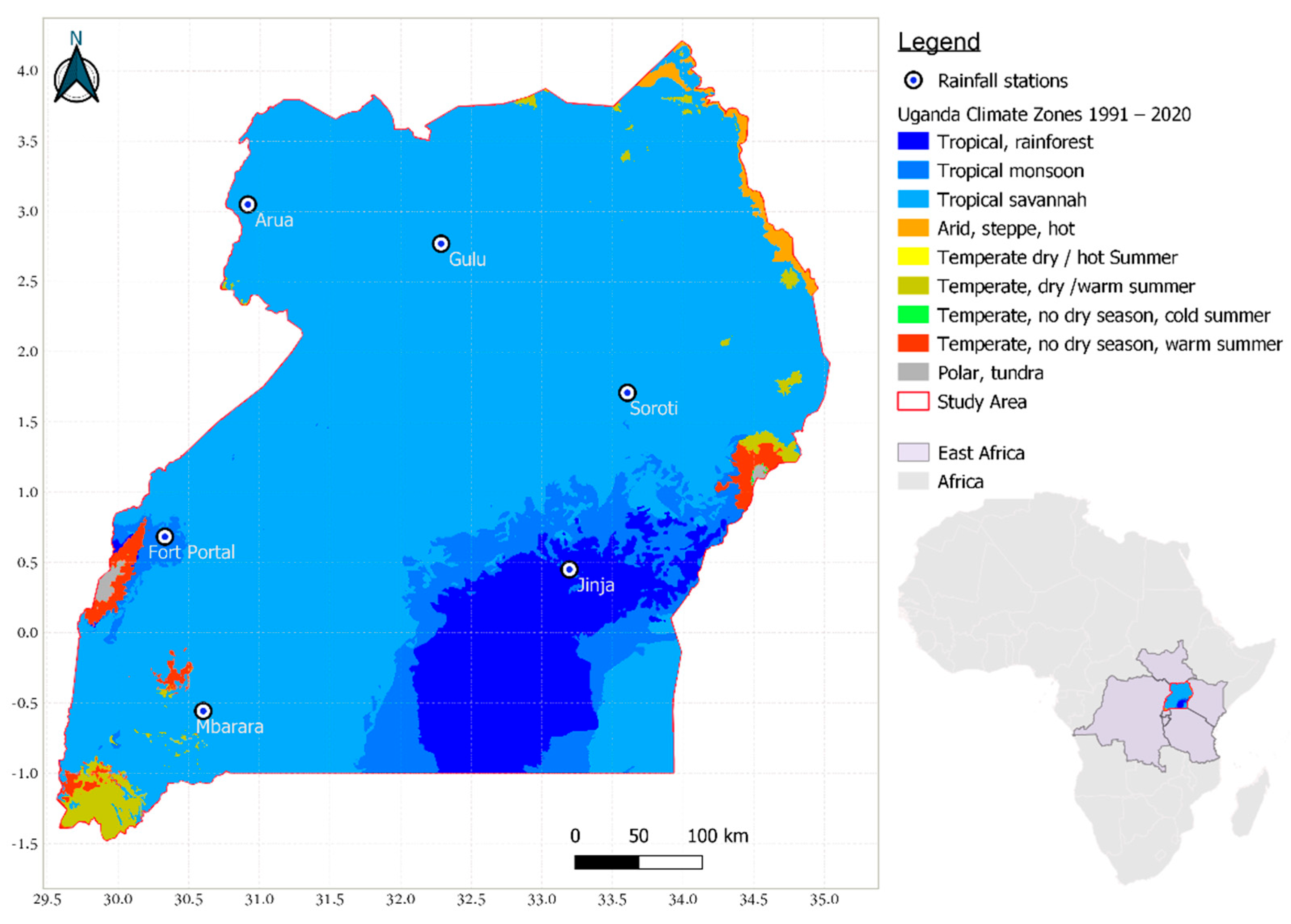
Figure 2.
Gaps in rainfall data at the Arua and the Fort Portal rainfall stations.
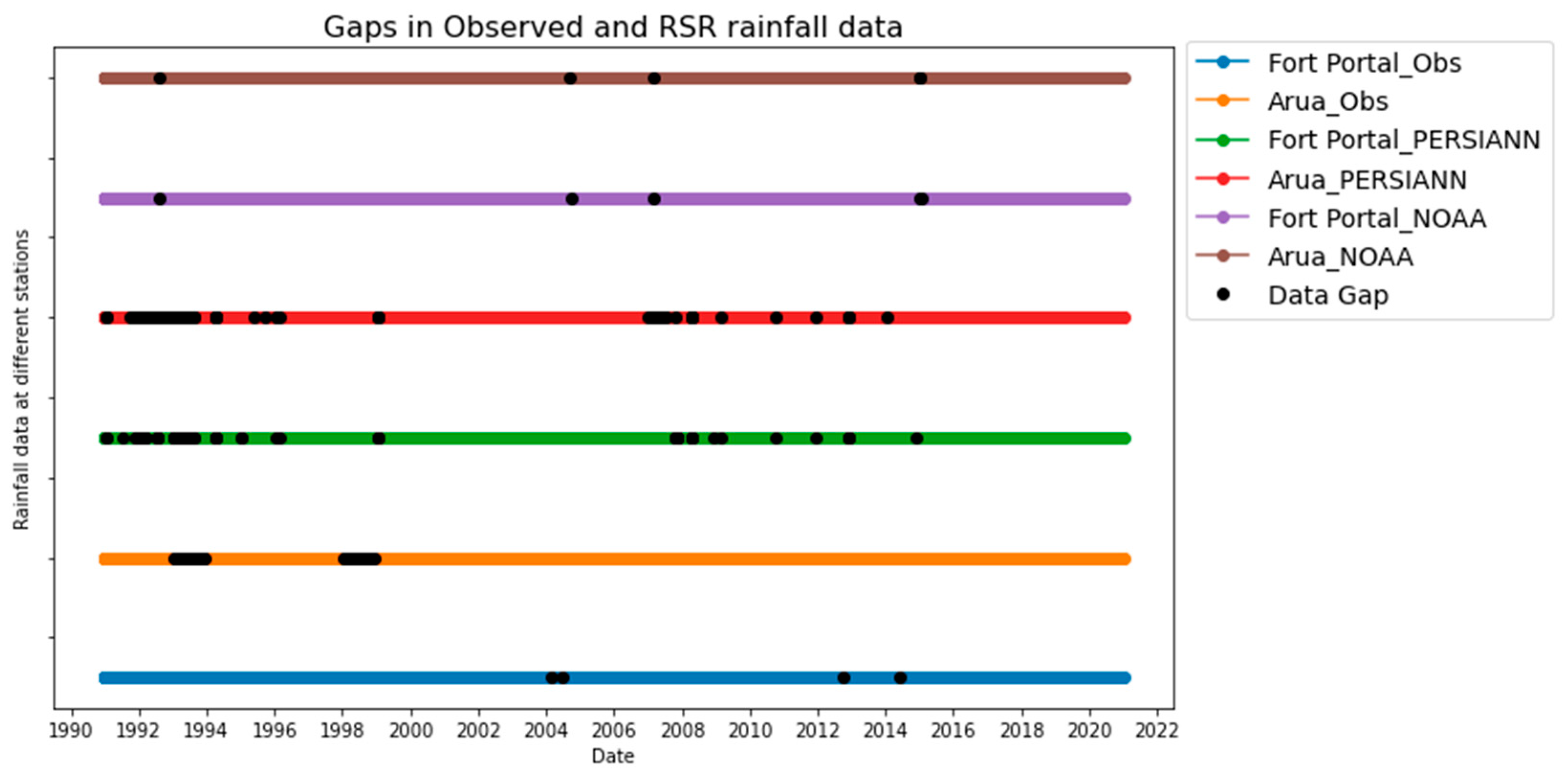
Figure 3.
Outlier detection at the Fort Portal station: (a) Time series plot and (b) IQR boxplot.
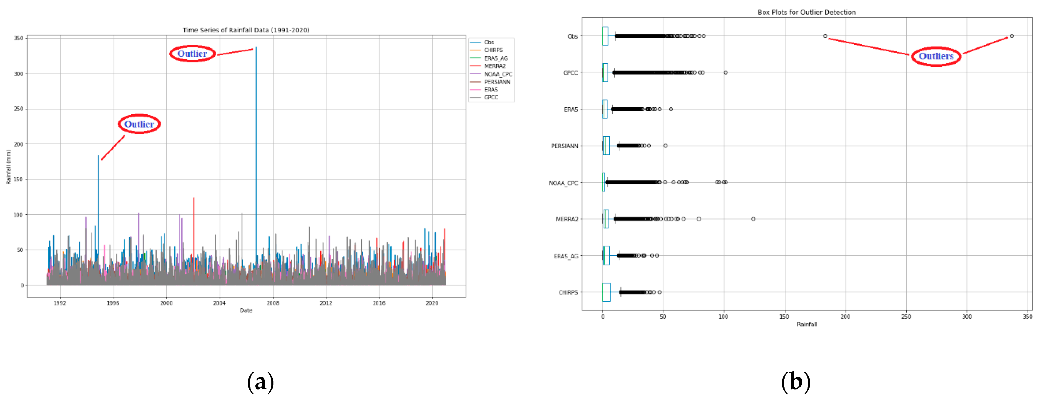
Figure 4.
Outlier detection at the Arua station: (a) From time series plot and (b) from IQR boxplot.
Figure 4.
Outlier detection at the Arua station: (a) From time series plot and (b) from IQR boxplot.
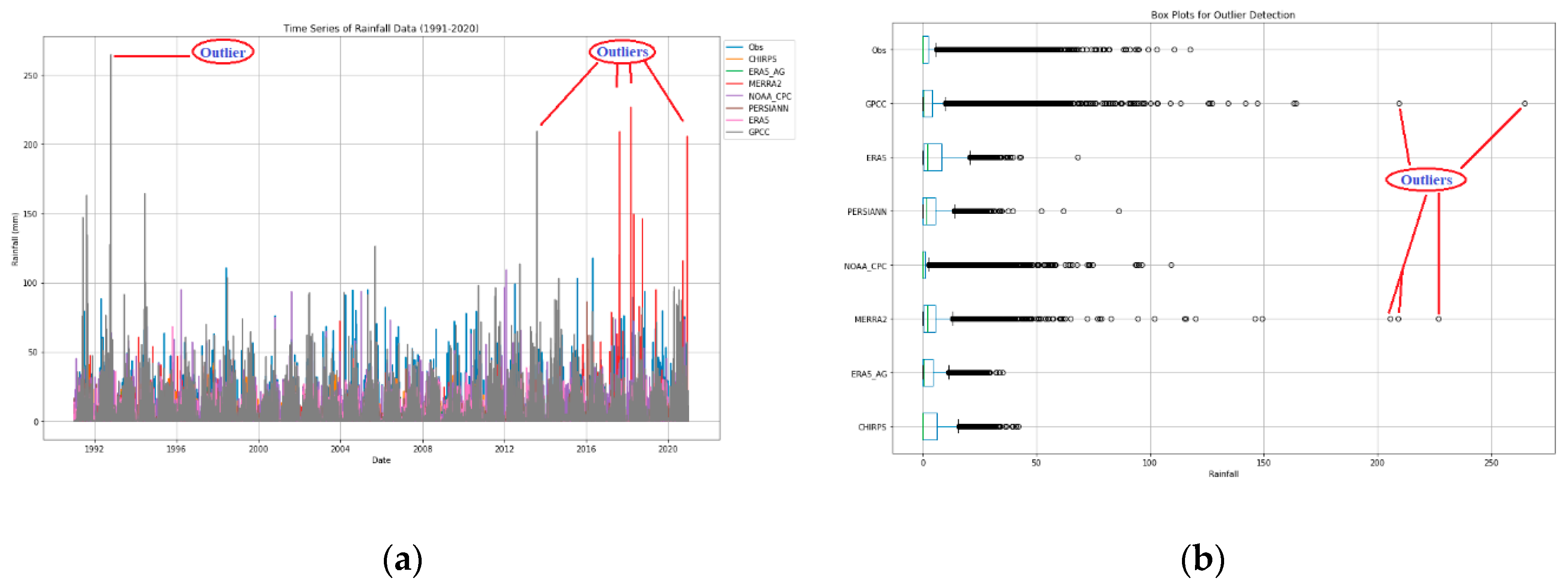
Figure 5.
Observed, original, and bias-corrected Rainfall at the Gulu Station.
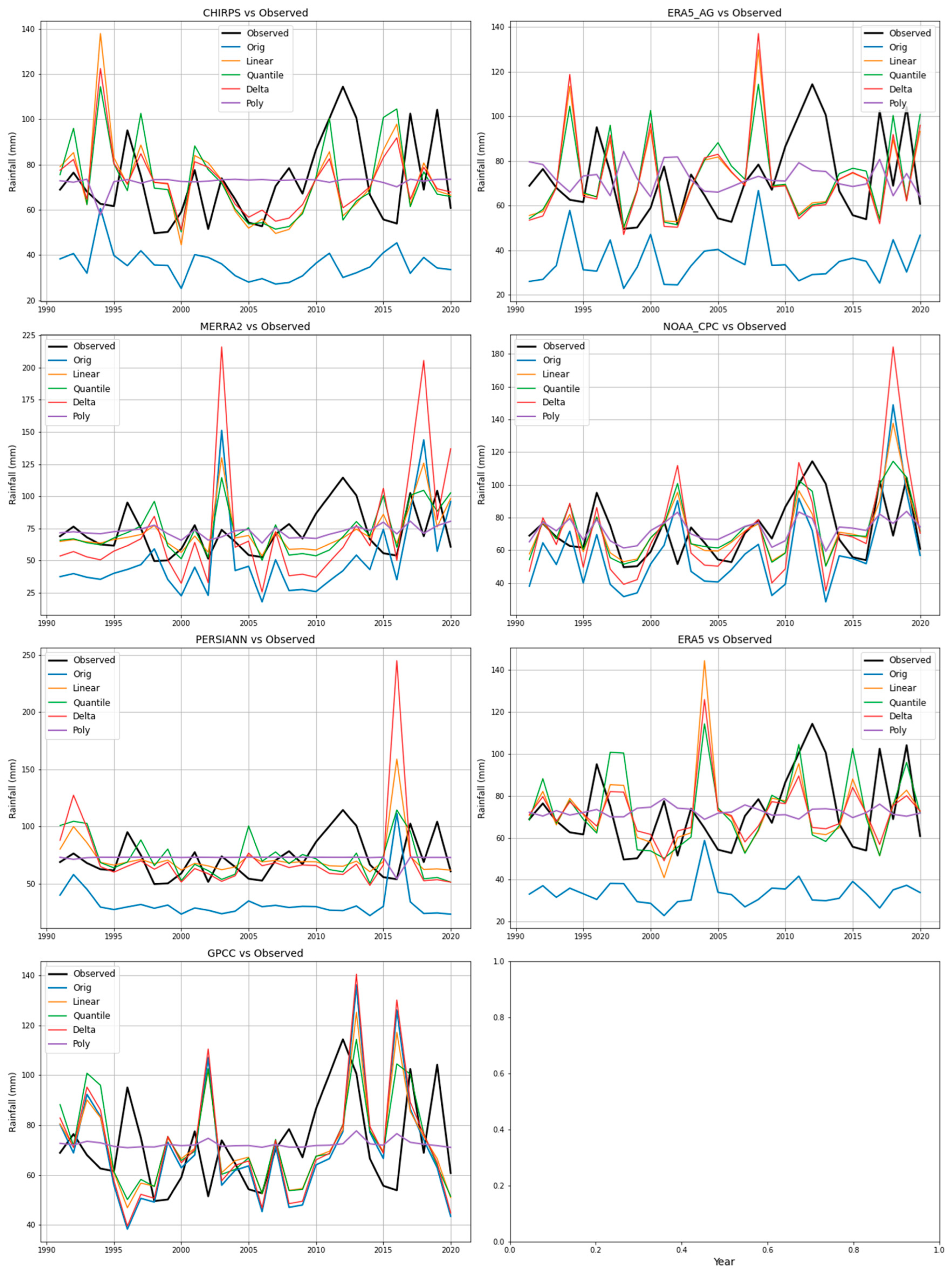
Figure 6.
Observed, original, and bias-corrected Rainfall at the Soroti Station.
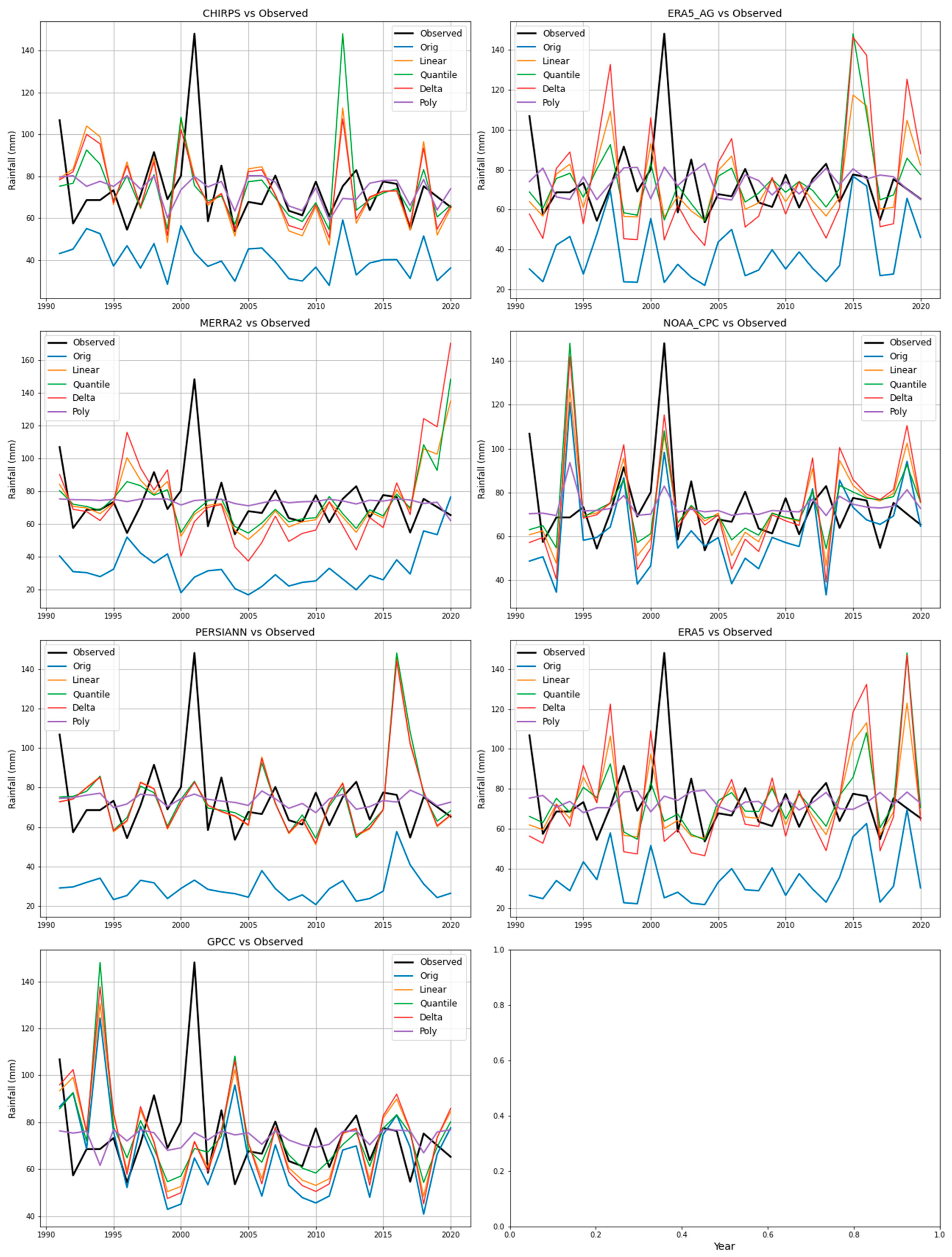
Figure 7.
Observed, original, and bias-corrected Rainfall at the Jinja Station.
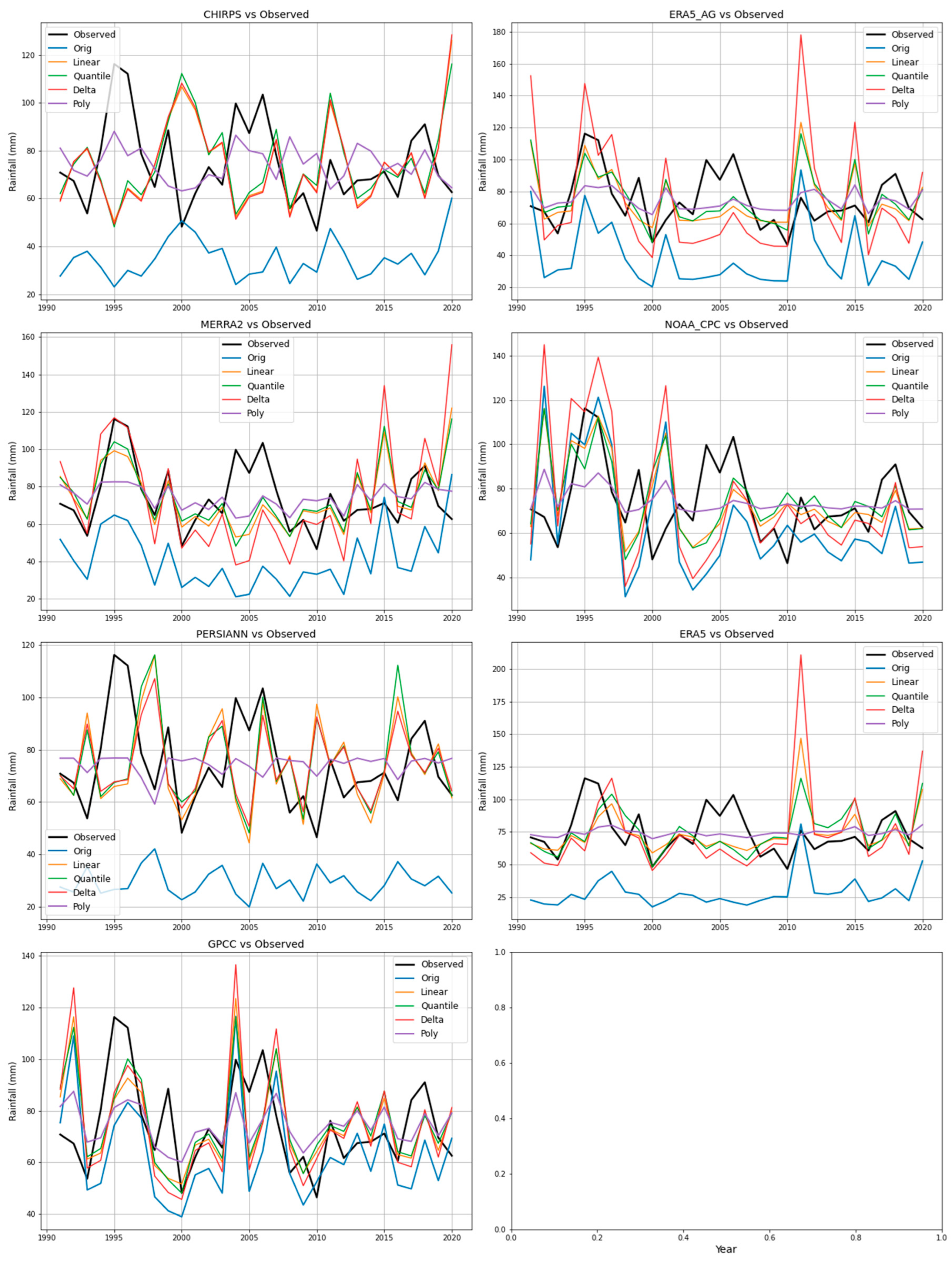
Figure 8.
Observed, original, and bias-corrected Rainfall at the Mbarara Station.
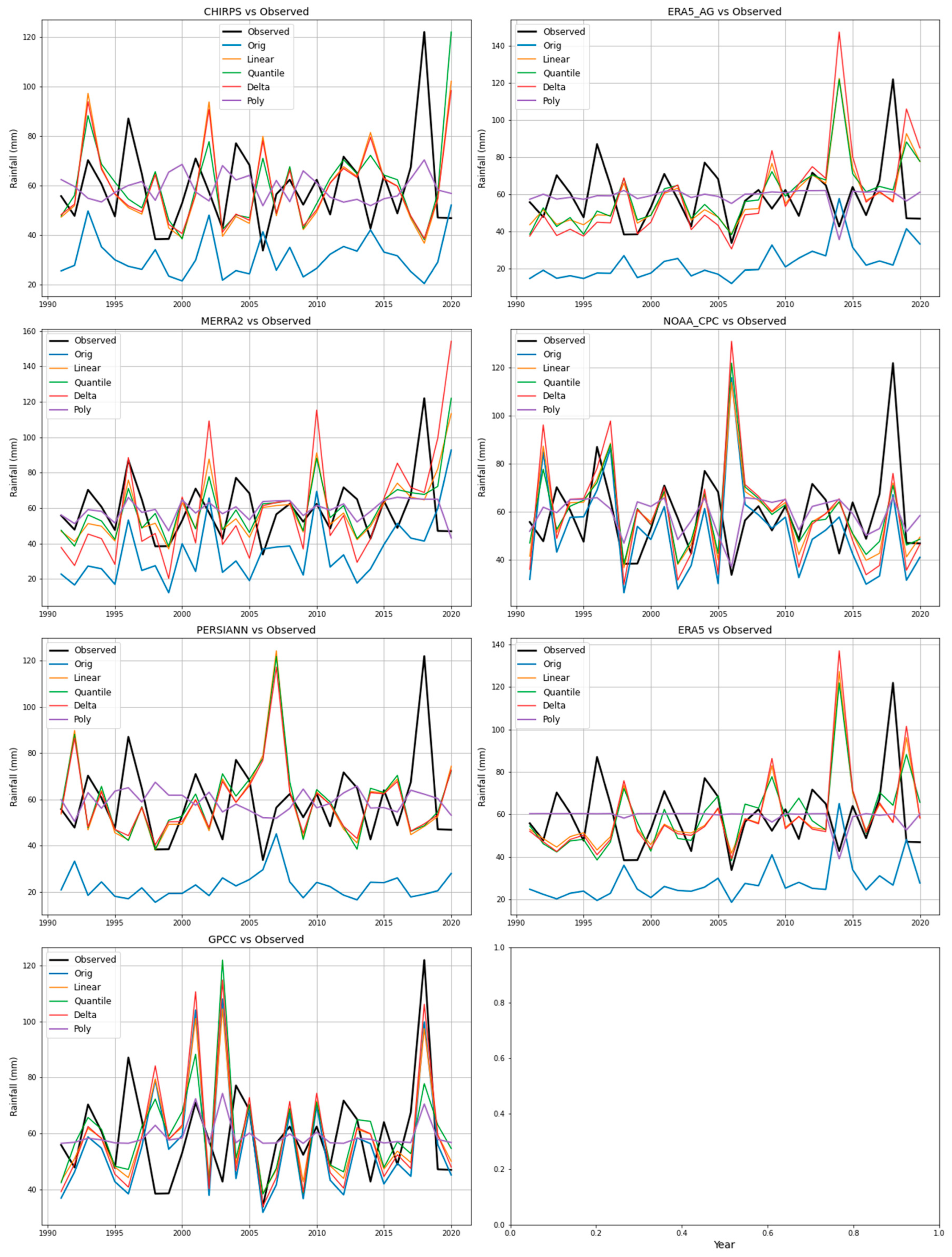
Figure 9.
PDF and CDF of observed and bias-corrected data for the Gulu station.
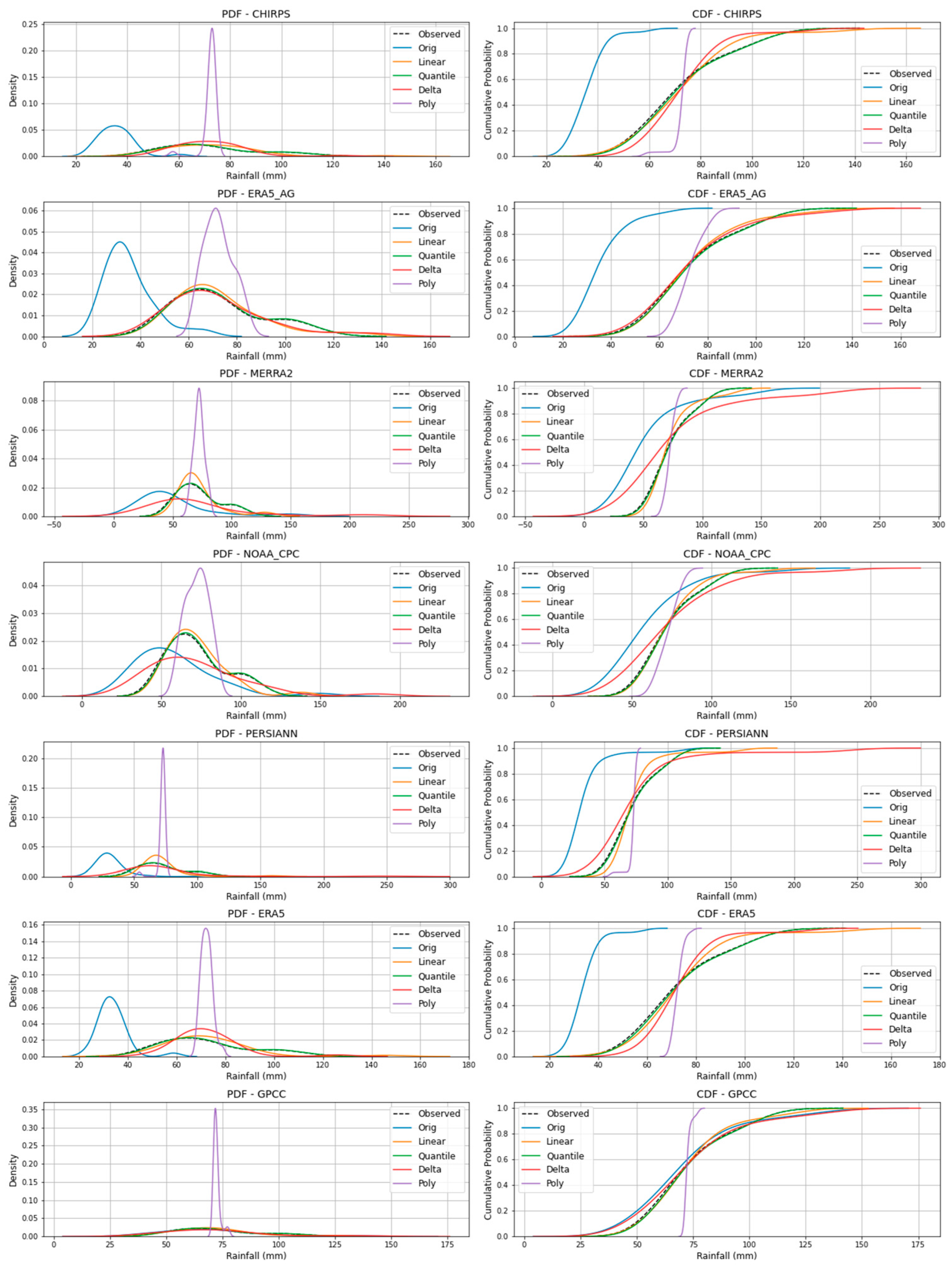
Figure 10.
PDF and CDF of observed and bias-corrected data for the Soroti station.
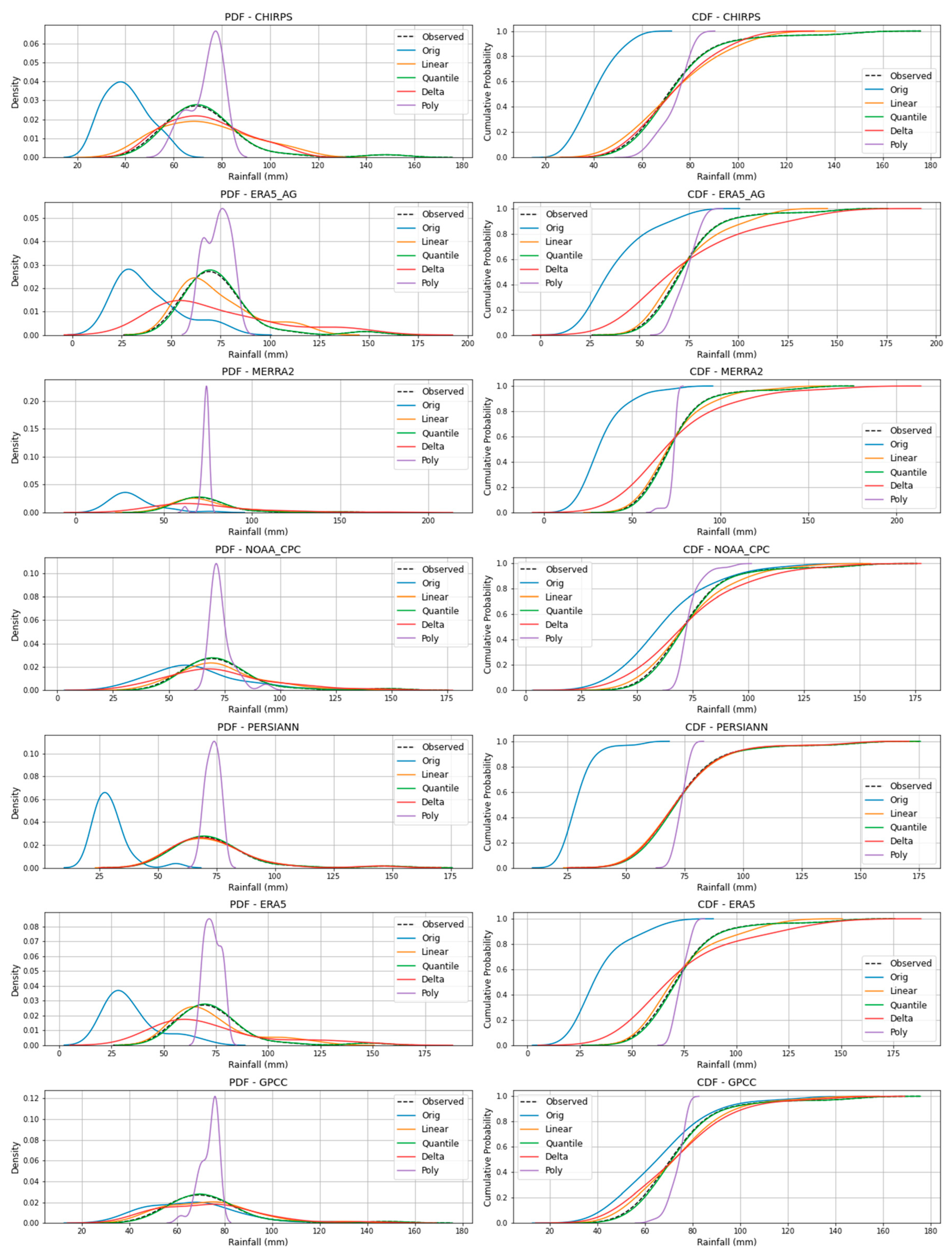
Figure 11.
PDF and CDF of observed and bias-corrected data for the Jinja station.
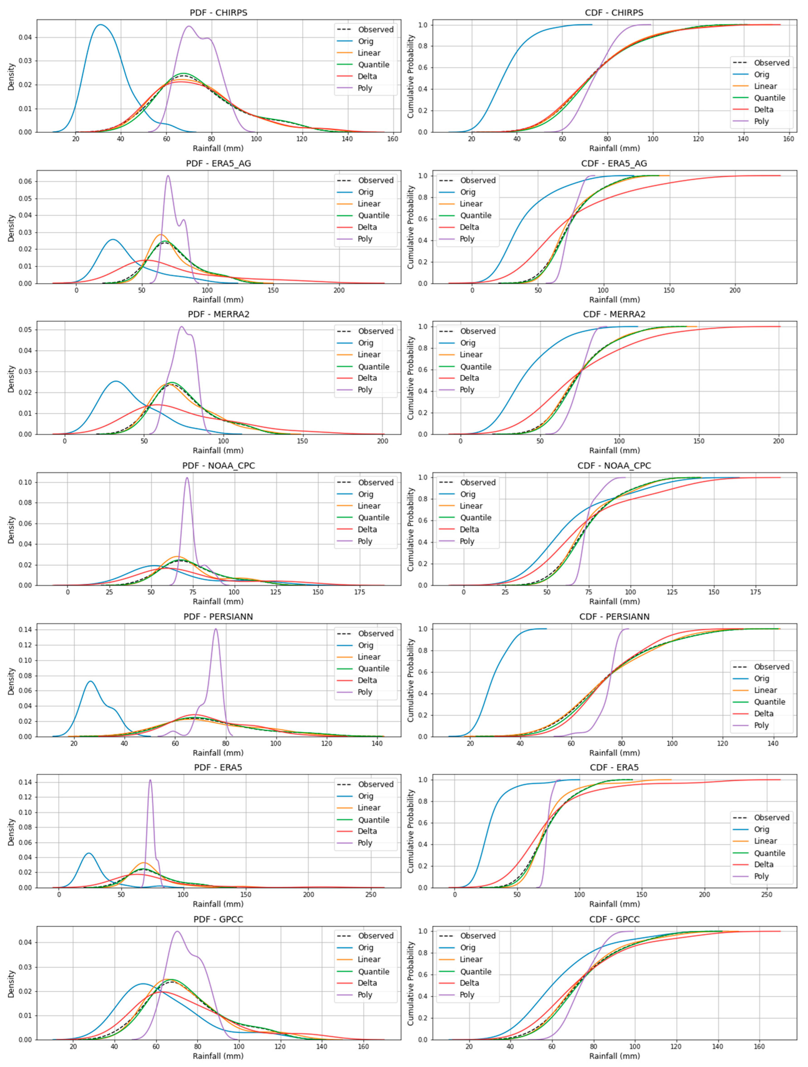
Figure 12.
PDF and CDF of observed and bias-corrected data for the Mbarara station.
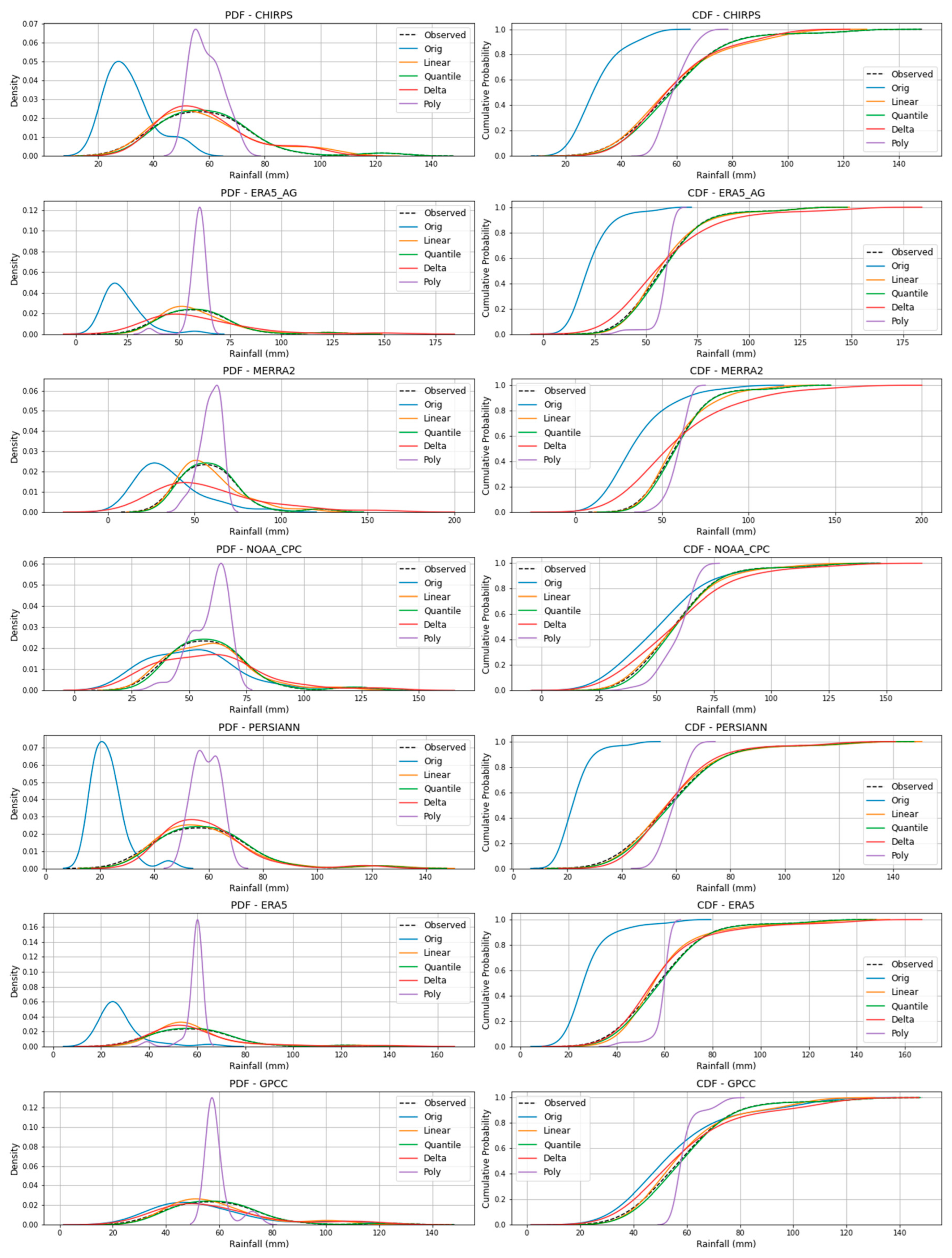
Figure 13.
A flow chart of the proposed RSR data bias correction framework.
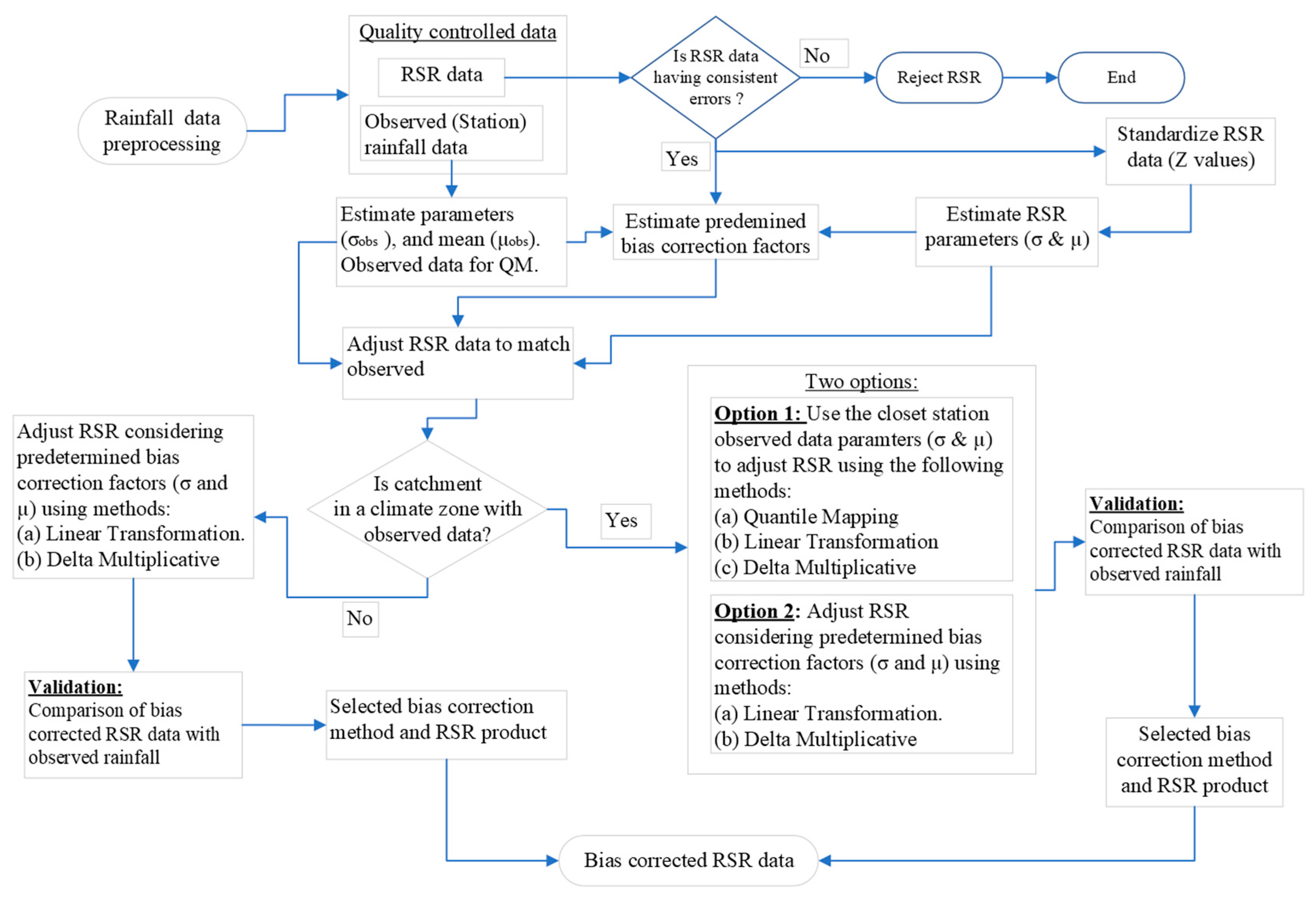
Figure 14.
Variation of biases in standard deviation of the rainfall datasets.
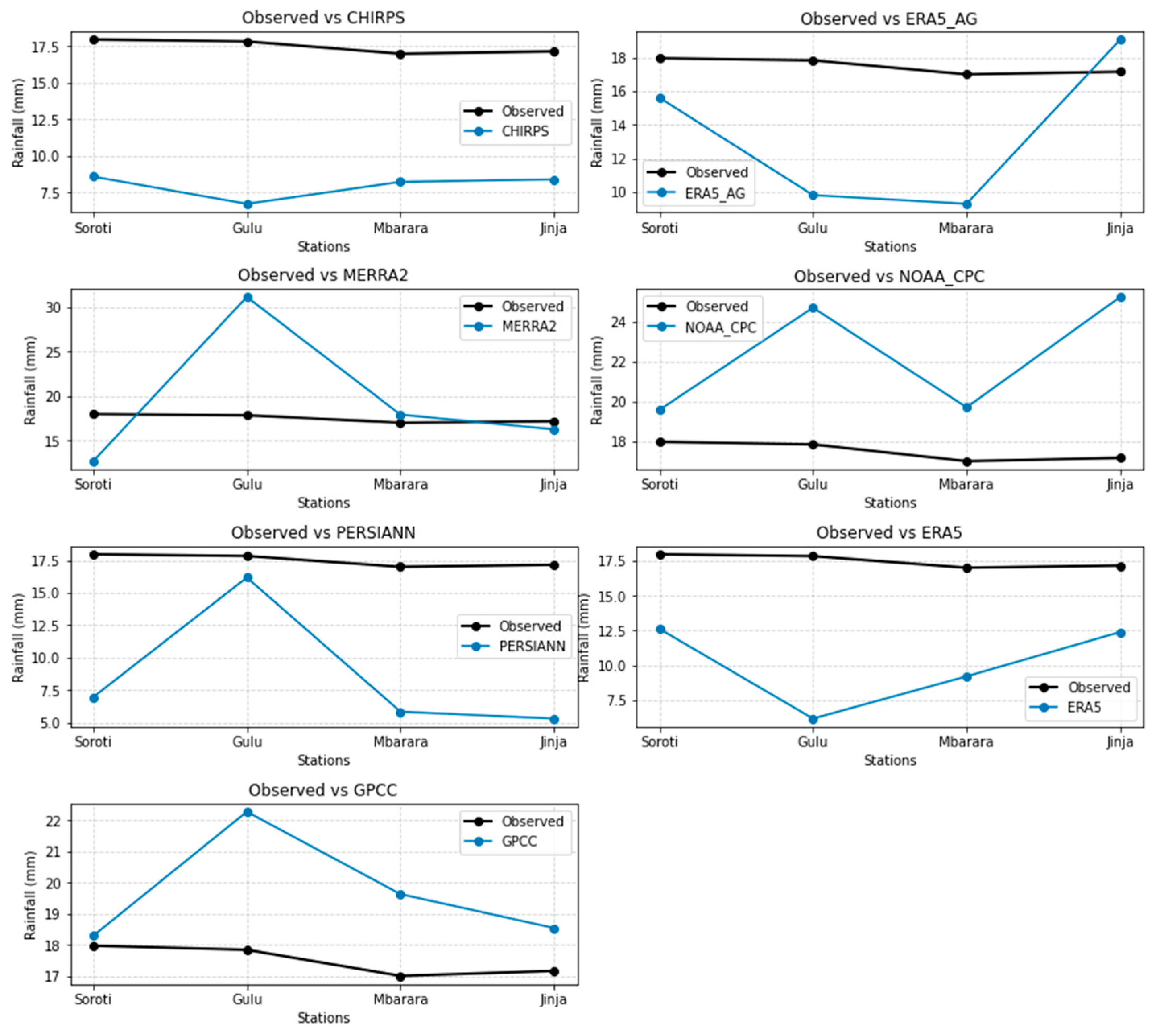
Figure 15.
Variation of biases in the means of the rainfall datasets.
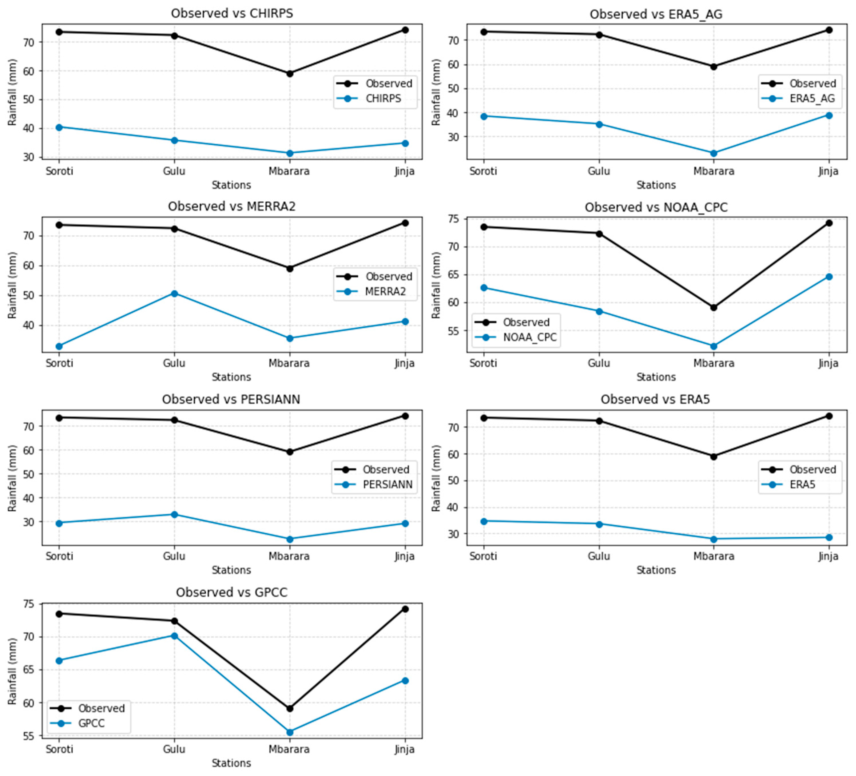
Figure 16.
Observed, original and bias-corrected rainfall at the Arua station.
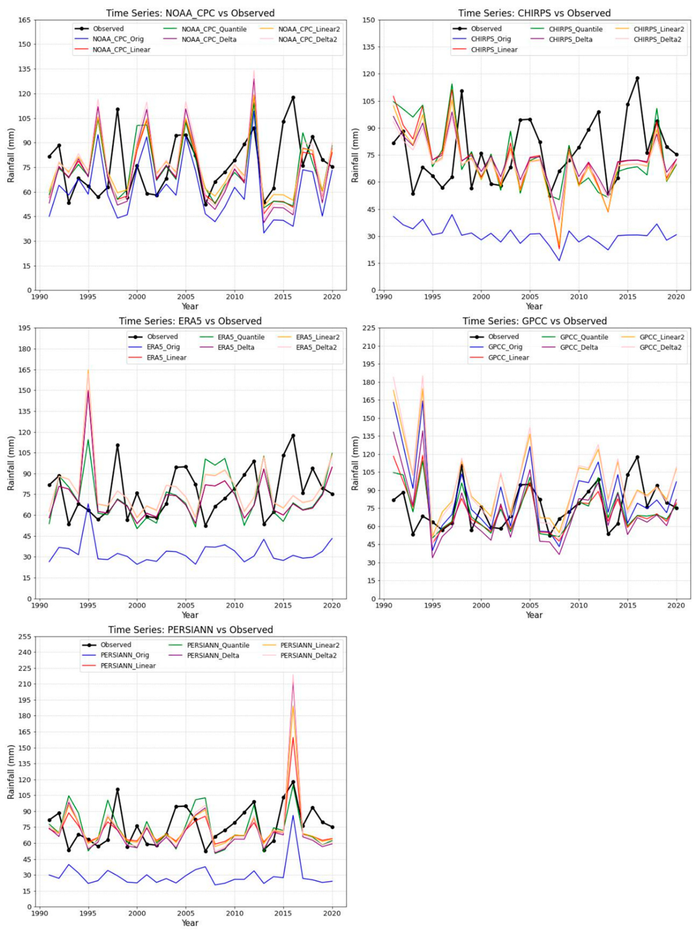
Figure 17.
Observed, original and bias-corrected rainfall at the Fort Portal station.
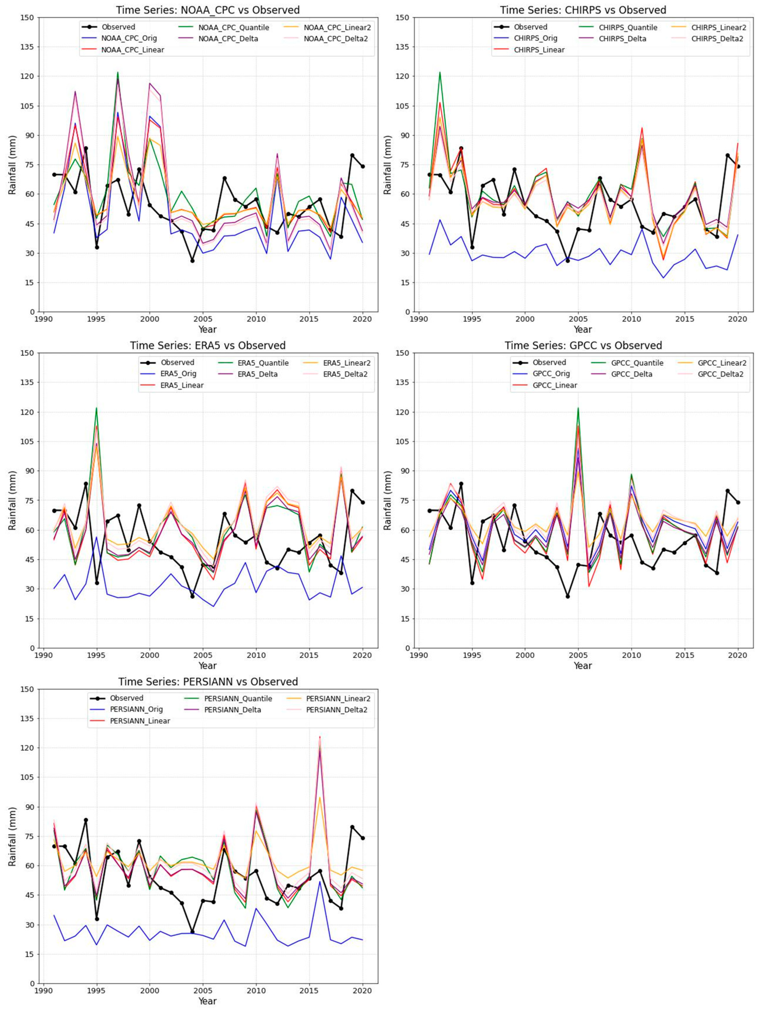
Figure 18.
PDF and CDF of observed and bias-corrected data for the Arua station.
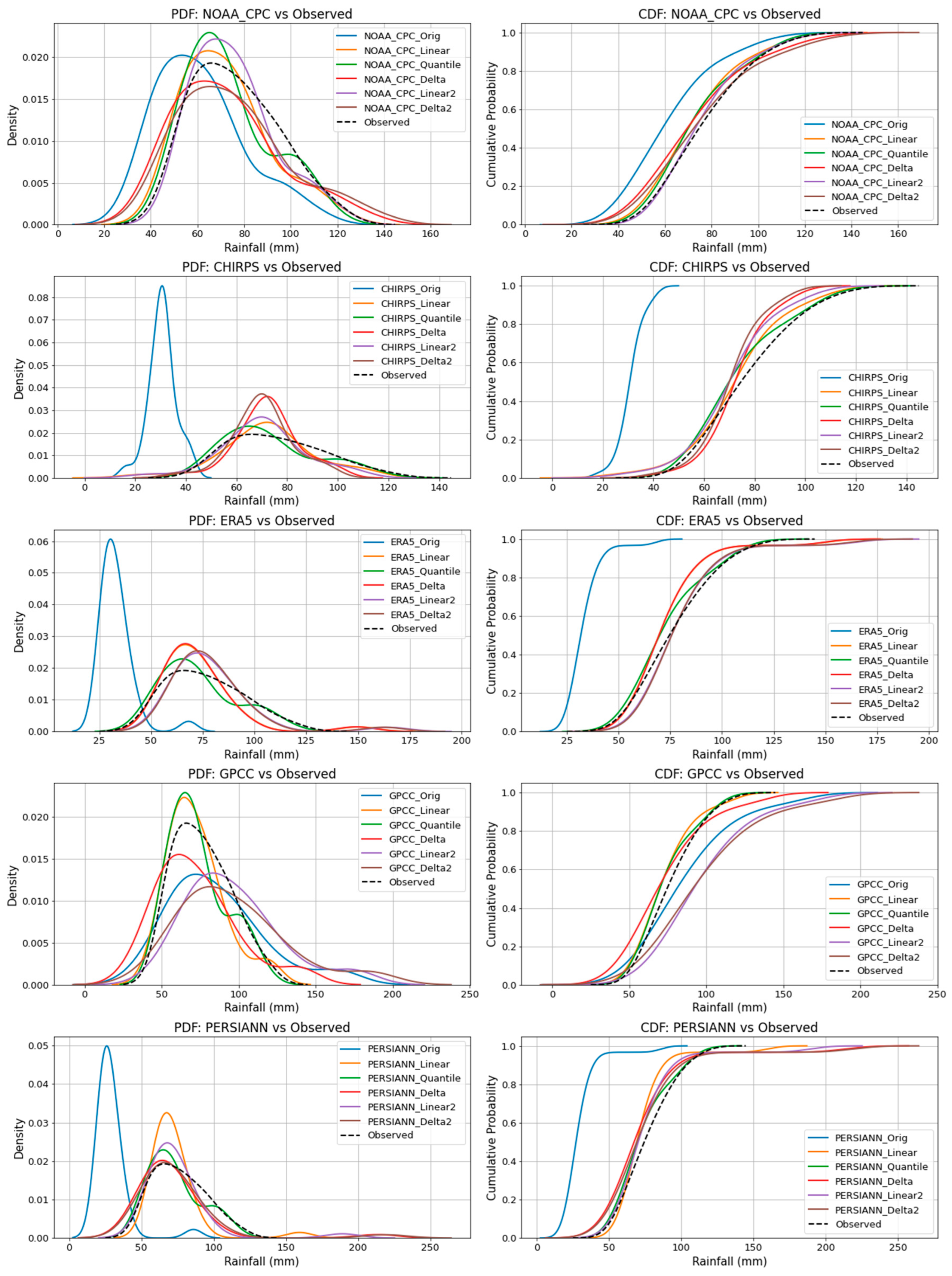
Figure 19.
PDF and CDF of observed and bias-corrected data for the Fort Portal station.
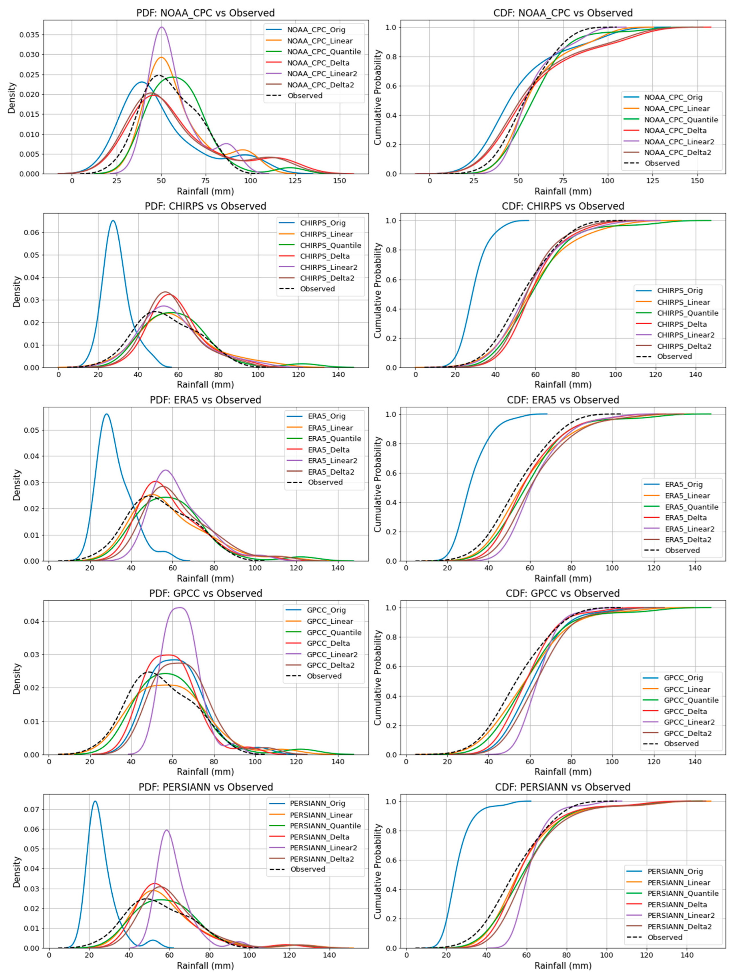

Table 1.
Equation for estimating PERSIANN RSR data missing rainfall values.
| Station | Regression Equation | R2 value |
|---|---|---|
| Arua | y = 1.3804x | 0.9962 |
| Fort Portal | y = 1.5565x | 0.9976 |
Table 2.
Equations for statistical performance metrics.
| Equation | Range (remarks) | Optimum value (units) |
|---|---|---|
| 0 to ∞ (smaller is better) | 0 (mm) | |
| 0 to ∞ (smaller is better) | 0 (mm) | |
| -∞ to ∞ (closer to 0 is better) | 0 (%) | |
| -∞ to 1 (closer to 1 is better) | 1 ( ) |
Where: Robs,i is the observed rainfall values, Radj,i is the bias corrected RSR values, and is the mean of the observed rainfall data.
Table 3.
Statistical performance test results at the Gulu and the Soroti stations.
| Dataset / Bias correction Method | Gulu station | Soroti Station | ||||||
|---|---|---|---|---|---|---|---|---|
| RMSE | MAE | PBIAS | NSE | RMSE | MAE | PBIAS | NSE | |
| NOAA_CPC_Orig | 29.20 | 22.44 | -19.23 | -1.68 | 25.24 | 19.03 | -14.79 | -0.97 |
| NOAA_CPC_Linear | 21.03 | 13.98 | 0.00 | -0.39 | 21.78 | 16.60 | 0.00 | -0.47 |
| NOAA_CPC_Quantile | 19.00 | 12.84 | 1.05 | -0.14 | 21.79 | 14.99 | 0.90 | -0.47 |
| NOAA_CPC_Delta | 30.33 | 18.80 | 0.00 | -1.89 | 25.12 | 18.99 | 0.00 | -0.95 |
| NOAA_CPC_Poly | 16.43 | 13.06 | 0.00 | 0.15 | 17.25 | 11.73 | 0.00 | 0.08 |
| CHIRPS_Orig | 41.64 | 36.61 | -50.59 | -4.45 | 37.67 | 33.07 | -45.00 | -3.39 |
| CHIRPS_Linear | 26.74 | 20.45 | 0.00 | -1.25 | 22.27 | 17.09 | 0.00 | -0.54 |
| CHIRPS_Quantile | 26.12 | 19.97 | 1.05 | -1.14 | 23.18 | 15.58 | 0.90 | -0.66 |
| CHIRPS_Delta | 23.75 | 18.20 | -0.01 | -0.77 | 20.89 | 15.68 | 0.00 | -0.35 |
| CHIRPS_Poly | 17.62 | 14.33 | 0.00 | 0.02 | 16.75 | 10.94 | 0.00 | 0.13 |
| ERA5_Orig | 43.29 | 38.66 | -53.41 | -4.89 | 45.03 | 38.76 | -52.74 | -5.28 |
| ERA5_Linear | 26.52 | 19.66 | 0.00 | -1.21 | 26.59 | 18.97 | 0.00 | -1.19 |
| ERA5_Quantile | 25.53 | 19.31 | 1.05 | -1.05 | 26.46 | 17.69 | 0.90 | -1.17 |
| ERA5_Delta | 23.32 | 17.95 | 0.00 | -0.71 | 33.57 | 24.68 | 0.00 | -2.49 |
| ERA5_Poly | 17.70 | 14.18 | 0.00 | 0.02 | 17.61 | 11.35 | 0.00 | 0.04 |
| GPCC_Orig | 27.46 | 21.15 | -3.05 | -1.37 | 26.08 | 18.90 | -9.66 | -1.10 |
| GPCC_Linear | 24.16 | 18.64 | 0.00 | -0.84 | 24.88 | 17.11 | 0.00 | -0.92 |
| GPCC_Quantile | 23.66 | 18.41 | 1.05 | -0.76 | 26.19 | 16.32 | 0.90 | -1.12 |
| GPCC_Delta | 27.91 | 21.36 | 0.00 | -1.45 | 26.50 | 18.36 | -0.01 | -1.17 |
| GPCC_Poly | 17.77 | 14.46 | 0.00 | 0.01 | 17.58 | 11.61 | 0.00 | 0.04 |
| PERSIANN_Orig | 47.30 | 43.28 | -54.50 | -6.03 | 47.80 | 44.02 | -59.89 | -6.07 |
| PERSIANN_Linear | 27.35 | 18.46 | 0.00 | -1.35 | 24.18 | 17.43 | 0.00 | -0.81 |
| PERSIANN_Quantile | 26.20 | 21.24 | 1.05 | -1.16 | 24.27 | 17.00 | 0.90 | -0.82 |
| PERSIANN_Delta | 42.49 | 25.29 | 0.00 | -4.68 | 23.77 | 17.14 | 0.00 | -0.75 |
| PERSIANN_Poly | 17.51 | 13.97 | 0.00 | 0.04 | 17.74 | 11.86 | 0.00 | 0.03 |
| ERA5_AG_Orig | 43.28 | 37.14 | -51.32 | -4.89 | 43.30 | 35.02 | -47.65 | -4.80 |
| ERA5_AG_Linear | 27.94 | 22.49 | 0.00 | -1.45 | 27.21 | 20.42 | 0.00 | -1.29 |
| ERA5_AG_Quantile | 28.50 | 23.51 | 1.05 | -1.55 | 26.80 | 18.41 | 0.90 | -1.22 |
| ERA5_AG_Delta | 29.74 | 23.88 | 0.00 | -1.78 | 37.00 | 29.34 | 0.00 | -3.24 |
| ERA5_AG_Poly | 16.90 | 13.09 | 0.00 | 0.10 | 16.98 | 10.23 | 0.00 | 0.11 |
| MERRA2_Orig | 40.75 | 36.07 | -30.01 | -4.22 | 46.41 | 41.27 | -55.16 | -5.67 |
| MERRA2_Linear | 24.07 | 17.62 | 0.00 | -0.82 | 26.13 | 18.29 | 0.00 | -1.11 |
| MERRA2_Quantile | 23.55 | 17.32 | 1.05 | -0.74 | 26.03 | 17.43 | 0.90 | -1.10 |
| MERRA2_Delta | 46.43 | 31.70 | 0.00 | -5.78 | 34.37 | 24.41 | 0.00 | -2.66 |
| MERRA2_Poly | 17.32 | 13.99 | 0.00 | 0.06 | 17.81 | 11.55 | 0.00 | 0.02 |
Table 4.
Statistical performance test results at the Jinja and the Mbarara stations.
| Dataset / Bias correction Method | Jinja station | Mbarara Station | ||||||
|---|---|---|---|---|---|---|---|---|
| RMSE | MAE | PBIAS | NSE | RMSE | MAE | PBIAS | NSE | |
| NOAA_CPC_Orig | 27.63 | 23.42 | -12.93 | -1.59 | 25.77 | 19.51 | -11.63 | -1.30 |
| NOAA_CPC_Linear | 20.30 | 15.79 | 0.00 | -0.40 | 22.93 | 15.97 | 0.00 | -0.82 |
| NOAA_CPC_Quantile | 21.13 | 16.33 | 1.25 | -0.52 | 23.11 | 15.05 | 1.43 | -0.85 |
| NOAA_CPC_Delta | 28.91 | 22.04 | 0.00 | -1.84 | 26.79 | 18.59 | 0.00 | -1.48 |
| NOAA_CPC_Poly | 16.35 | 12.82 | 0.00 | 0.09 | 15.34 | 11.20 | 0.00 | 0.19 |
| CHIRPS_Orig | 45.09 | 39.64 | -53.18 | -5.90 | 34.56 | 28.61 | -46.99 | -3.13 |
| CHIRPS_Linear | 28.52 | 21.79 | 0.00 | -1.76 | 26.77 | 19.33 | -0.01 | -1.48 |
| CHIRPS_Quantile | 28.24 | 21.38 | 1.25 | -1.71 | 26.41 | 18.43 | 1.43 | -1.41 |
| CHIRPS_Delta | 29.17 | 22.33 | 0.00 | -1.89 | 25.63 | 18.44 | -0.01 | -1.27 |
| CHIRPS_Poly | 15.63 | 12.40 | 0.00 | 0.17 | 16.18 | 12.90 | 0.01 | 0.09 |
| ERA5_Orig | 50.04 | 46.03 | -61.57 | -7.50 | 37.48 | 32.59 | -52.53 | -3.86 |
| ERA5_Linear | 23.32 | 16.98 | 0.00 | -0.85 | 26.54 | 17.90 | 0.00 | -1.44 |
| ERA5_Quantile | 22.45 | 17.23 | 1.25 | -0.71 | 25.07 | 16.97 | 1.43 | -1.17 |
| ERA5_Delta | 35.35 | 22.34 | 0.00 | -3.24 | 28.45 | 18.86 | 0.00 | -1.80 |
| ERA5_Poly | 16.95 | 13.61 | 0.00 | 0.02 | 16.52 | 11.74 | 0.00 | 0.06 |
| GPCC_Orig | 22.22 | 17.56 | -14.64 | -0.68 | 22.62 | 16.60 | -5.93 | -0.77 |
| GPCC_Linear | 18.60 | 14.80 | 0.00 | -0.17 | 20.66 | 14.98 | 0.00 | -0.48 |
| GPCC_Quantile | 17.96 | 14.36 | 1.25 | -0.10 | 22.72 | 15.85 | 1.43 | -0.79 |
| GPCC_Delta | 21.42 | 16.65 | 0.00 | -0.56 | 23.21 | 16.50 | 0.00 | -0.86 |
| GPCC_Poly | 15.42 | 12.53 | 0.00 | 0.19 | 16.34 | 11.94 | 0.00 | 0.08 |
| PERSIANN_Orig | 48.88 | 45.10 | -60.76 | -7.11 | 41.10 | 36.33 | -61.51 | -4.84 |
| PERSIANN_Linear | 26.36 | 20.30 | 0.00 | -1.36 | 26.66 | 18.71 | 0.00 | -1.46 |
| PERSIANN_Quantile | 25.68 | 19.59 | 1.25 | -1.24 | 26.35 | 18.55 | 1.43 | -1.40 |
| PERSIANN_Delta | 23.68 | 18.24 | 0.00 | -0.90 | 25.26 | 17.76 | 0.00 | -1.21 |
| PERSIANN_Poly | 16.73 | 13.33 | 0.00 | 0.05 | 16.39 | 12.13 | 0.00 | 0.07 |
| ERA5_AG_Orig | 41.30 | 37.04 | -47.51 | -4.79 | 41.36 | 36.94 | -60.85 | -4.92 |
| ERA5_AG_Linear | 20.32 | 16.57 | 0.00 | -0.40 | 25.65 | 17.79 | 0.00 | -1.28 |
| ERA5_AG_Quantile | 18.87 | 15.36 | 1.25 | -0.21 | 24.80 | 17.29 | 1.21 | -1.13 |
| ERA5_AG_Delta | 35.24 | 27.79 | 0.00 | -3.22 | 31.01 | 21.32 | 0.00 | -2.33 |
| ERA5_AG_Poly | 16.11 | 13.30 | 0.00 | 0.12 | 16.32 | 11.77 | 0.00 | 0.08 |
| MERRA2_Orig | 38.52 | 34.87 | -44.57 | -4.04 | 33.35 | 28.83 | -39.85 | -2.85 |
| MERRA2_Linear | 20.25 | 14.77 | 0.00 | -0.39 | 23.00 | 16.99 | 0.00 | -0.83 |
| MERRA2_Quantile | 19.63 | 14.21 | 1.25 | -0.31 | 22.51 | 16.35 | 1.43 | -0.75 |
| MERRA2_Delta | 29.12 | 19.69 | 0.00 | -1.88 | 33.02 | 24.28 | 0.00 | -2.77 |
| MERRA2_Poly | 16.03 | 12.90 | 0.00 | 0.13 | 15.98 | 11.53 | 0.00 | 0.12 |
Table 5.
Goodness-of-Fit test results for the four gauged stations.
| Dataset / Bias correction Method | Gulu station | Soroti station | Jinja station | Mbarara station | ||||
|---|---|---|---|---|---|---|---|---|
| KS | p-value | KS | p-value | KS | p-value | KS | p-value | |
| NOAA_CPC_Orig | 0.40 | 0.02 | 0.40 | 0.02 | 0.50 | 0.00 | 0.27 | 0.24 |
| NOAA_CPC_Linear | 0.13 | 0.96 | 0.13 | 0.96 | 0.13 | 0.96 | 0.13 | 0.96 |
| NOAA_CPC_Quantile | 0.03 | 1.00 | 0.03 | 1.00 | 0.03 | 1.00 | 0.03 | 1.00 |
| NOAA_CPC_Delta | 0.27 | 0.24 | 0.17 | 0.81 | 0.30 | 0.14 | 0.23 | 0.39 |
| NOAA_CPC_Poly | 0.27 | 0.24 | 0.50 | 0.00 | 0.47 | 0.00 | 0.27 | 0.24 |
| CHIRPS_Orig | 0.97 | 0.00 | 0.90 | 0.00 | 0.90 | 0.00 | 0.80 | 0.00 |
| CHIRPS_Linear | 0.13 | 0.96 | 0.20 | 0.59 | 0.13 | 0.96 | 0.10 | 1.00 |
| CHIRPS_Quantile | 0.03 | 1.00 | 0.03 | 1.00 | 0.03 | 1.00 | 0.03 | 1.00 |
| CHIRPS_Delta | 0.17 | 0.81 | 0.17 | 0.81 | 0.13 | 0.96 | 0.10 | 1.00 |
| CHIRPS_Poly | 0.53 | 0.00 | 0.30 | 0.14 | 0.30 | 0.14 | 0.37 | 0.03 |
| ERA5_Orig | 0.97 | 0.00 | 0.87 | 0.00 | 0.93 | 0.00 | 0.87 | 0.00 |
| ERA5_Linear | 0.13 | 0.96 | 0.17 | 0.81 | 0.20 | 0.59 | 0.23 | 0.39 |
| ERA5_Quantile | 0.03 | 1.00 | 0.03 | 1.00 | 0.03 | 1.00 | 0.03 | 1.00 |
| ERA5_Delta | 0.23 | 0.39 | 0.27 | 0.24 | 0.27 | 0.24 | 0.23 | 0.39 |
| ERA5_Poly | 0.53 | 0.00 | 0.40 | 0.02 | 0.50 | 0.00 | 0.47 | 0.00 |
| GPCC_Orig | 0.20 | 0.59 | 0.37 | 0.03 | 0.43 | 0.01 | 0.30 | 0.14 |
| GPCC_Linear | 0.10 | 1.00 | 0.20 | 0.59 | 0.10 | 1.00 | 0.20 | 0.59 |
| GPCC_Quantile | 0.03 | 1.00 | 0.03 | 1.00 | 0.03 | 1.00 | 0.03 | 1.00 |
| GPCC_Delta | 0.17 | 0.81 | 0.23 | 0.39 | 0.20 | 0.59 | 0.20 | 0.59 |
| GPCC_Poly | 0.60 | 0.00 | 0.40 | 0.02 | 0.27 | 0.24 | 0.47 | 0.00 |
| PERSIANN_Orig | 0.93 | 0.00 | 0.97 | 0.00 | 1.00 | 0.00 | 0.97 | 0.00 |
| PERSIANN_Linear | 0.30 | 0.14 | 0.10 | 1.00 | 0.10 | 1.00 | 0.13 | 0.96 |
| PERSIANN_Quantile | 0.03 | 1.00 | 0.03 | 1.00 | 0.03 | 1.00 | 0.03 | 1.00 |
| PERSIANN_Delta | 0.27 | 0.24 | 0.10 | 1.00 | 0.17 | 0.81 | 0.13 | 0.96 |
| PERSIANN_Poly | 0.57 | 0.00 | 0.47 | 0.00 | 0.43 | 0.01 | 0.37 | 0.03 |
| ERA5_AG_Orig | 0.93 | 0.00 | 0.83 | 0.00 | 0.73 | 0.00 | 0.93 | 0.00 |
| ERA5_AG_Linear | 0.13 | 0.96 | 0.20 | 0.59 | 0.17 | 0.81 | 0.13 | 0.96 |
| ERA5_AG_Quantile | 0.03 | 1.00 | 0.03 | 1.00 | 0.03 | 1.00 | 0.03 | 1.00 |
| ERA5_AG_Delta | 0.10 | 1.00 | 0.37 | 0.03 | 0.37 | 0.03 | 0.20 | 0.59 |
| ERA5_AG_Poly | 0.37 | 0.03 | 0.30 | 0.14 | 0.40 | 0.02 | 0.43 | 0.01 |
| MERRA2_Orig | 0.70 | 0.00 | 0.93 | 0.00 | 0.73 | 0.00 | 0.67 | 0.00 |
| MERRA2_Linear | 0.20 | 0.59 | 0.10 | 1.00 | 0.10 | 1.00 | 0.13 | 0.96 |
| MERRA2_Quantile | 0.03 | 1.00 | 0.03 | 1.00 | 0.03 | 1.00 | 0.03 | 1.00 |
| MERRA2_Delta | 0.30 | 0.14 | 0.20 | 0.59 | 0.27 | 0.24 | 0.33 | 0.07 |
| MERRA2_Poly | 0.37 | 0.03 | 0.53 | 0.00 | 0.30 | 0.14 | 0.30 | 0.14 |
Table 6.
Standard deviations of rainfall data at the four stations.
| Stations | Observed | CHIRPS | ERA5_AG | MERRA2 | NOAA | PERSIANN | ERA5 | GPCC |
|---|---|---|---|---|---|---|---|---|
| Soroti | 17.97 | 8.59 | 15.61 | 12.68 | 19.57 | 6.96 | 12.62 | 18.29 |
| Gulu | 17.84 | 6.73 | 9.79 | 31.14 | 24.69 | 16.18 | 6.18 | 22.28 |
| Mbarara | 17.00 | 8.23 | 9.27 | 17.91 | 19.70 | 5.84 | 9.21 | 19.63 |
| Jinja | 17.16 | 8.40 | 19.08 | 16.25 | 25.23 | 5.31 | 12.39 | 18.54 |
Table 7.
Predetermined bias correction factors in standard deviation data values.
| Stations | CHIRPS | ERA5_AG | MERRA2 | NOAA | PERSIANN | ERA5 | GPCC |
|---|---|---|---|---|---|---|---|
| Soroti | 9.39 | 2.36 | 5.29 | -1.60 | 11.01 | 5.35 | -0.32 |
| Gulu | 11.11 | 8.05 | -13.31 | -6.85 | 1.65 | 11.66 | -4.44 |
| Mbarara | 8.77 | 7.73 | -0.91 | -2.70 | 11.16 | 7.79 | -2.63 |
| Jinja | 8.76 | -1.92 | 0.91 | -8.07 | 11.85 | 4.77 | -1.38 |
| Maximum bias | 11.11 | -1.60 | 11.85 | 11.66 | -0.32 | ||
| Minimum bias | 8.76 | -8.07 | 1.65 | 4.77 | -4.44 |
Table 8.
Mean values of rainfalls at the four stations.
| Station | Observed | CHIRPS | ERA5_AG | MERRA2 | NOAA | PERSIANN | ERA5 | GPCC |
|---|---|---|---|---|---|---|---|---|
| Soroti | 73.49 | 40.42 | 38.47 | 32.95 | 62.62 | 29.48 | 34.74 | 66.39 |
| Gulu | 72.38 | 35.76 | 35.23 | 50.66 | 58.46 | 32.93 | 33.72 | 70.17 |
| Mbarara | 59.07 | 31.31 | 23.13 | 35.53 | 52.20 | 22.73 | 28.04 | 55.56 |
| Jinja | 74.23 | 34.75 | 38.97 | 41.15 | 64.63 | 29.13 | 28.53 | 63.36 |
Table 9.
Predetermined bias correction factors in mean rainfall values.
| Station | CHIRPS | ERA5_AG | MERRA2 | NOAA | PERSIANN | ERA5 | GPCC |
|---|---|---|---|---|---|---|---|
| Soroti | 33.07 | 35.02 | 40.54 | 10.87 | 44.02 | 38.76 | 7.10 |
| Gulu | 36.62 | 37.14 | 21.72 | 13.92 | 39.44 | 38.66 | 2.21 |
| Mbarara | 27.76 | 35.94 | 23.54 | 6.87 | 36.33 | 31.03 | 3.50 |
| Jinja | 39.48 | 35.26 | 33.08 | 9.60 | 45.10 | 45.70 | 10.87 |
| Maximum bias | 39.48 | 37.14 | 40.54 | 13.92 | 45.10 | 45.70 | 10.87 |
| Minimum bias | 27.76 | 35.02 | 21.72 | 6.87 | 36.33 | 31.03 | 2.21 |
Table 10.
Statistical performance validation results at the Arua and the Fort Portal stations.
| Dataset / Bias correction Method | Arua station | Fort Portal Station | ||||||
|---|---|---|---|---|---|---|---|---|
| RMSE | MAE | PBIAS | NSE | RMSE | MAE | PBIAS | NSE | |
| NOAA_CPC_Orig | 29.12 | 20.92 | -19.74 | -1.74 | 23.49 | 20.40 | -7.25 | -1.83 |
| NOAA_CPC_Linear | 24.90 | 18.23 | -5.32 | -1.00 | 20.18 | 15.40 | 8.39 | -1.09 |
| NOAA_CPC_Quantile | 25.16 | 19.07 | -4.32 | -1.04 | 18.91 | 14.64 | 9.94 | -0.83 |
| NOAA_CPC_Delta | 27.63 | 20.58 | -5.32 | -1.47 | 26.58 | 20.07 | 8.39 | -2.62 |
| NOAA_CPC_Linear2 | 23.82 | 17.76 | -1.53 | -0.83 | 17.56 | 14.08 | 5.36 | -0.58 |
| NOAA_CPC_Delta2 | 28.02 | 21.14 | -1.53 | -1.54 | 25.75 | 20.04 | 5.36 | -2.40 |
| CHIRPS_Orig | 49.14 | 45.74 | -59.83 | -6.80 | 28.35 | 25.28 | -46.20 | -3.12 |
| CHIRPS_Linear | 24.48 | 19.73 | -5.32 | -0.94 | 18.17 | 13.11 | 8.39 | -0.69 |
| CHIRPS_Quantile | 25.83 | 21.00 | -4.34 | -1.15 | 18.24 | 12.64 | 9.94 | -0.71 |
| CHIRPS_Delta | 21.07 | 17.23 | -5.31 | -0.43 | 15.68 | 11.89 | 8.39 | -0.26 |
| CHIRPS_Linear2 | 23.94 | 19.26 | -8.18 | -0.85 | 16.53 | 12.24 | 4.73 | -0.40 |
| CHIRPS_Delta2 | 21.41 | 17.38 | -8.18 | -0.48 | 15.02 | 11.35 | 4.74 | -0.16 |
| ERA5_Orig | 48.14 | 43.67 | -56.72 | -6.49 | 28.75 | 24.84 | -41.17 | -3.24 |
| ERA5_Linear | 27.99 | 21.07 | -5.32 | -1.53 | 25.64 | 19.75 | 8.39 | -2.37 |
| ERA5_Quantile | 28.12 | 22.47 | -4.32 | -1.55 | 25.37 | 18.84 | 9.94 | -2.30 |
| ERA5_Delta | 27.83 | 20.99 | -5.32 | -1.50 | 23.33 | 18.06 | 8.39 | -1.79 |
| ERA5_Linear2 | 29.29 | 21.93 | 3.06 | -1.77 | 23.15 | 17.36 | 15.77 | -1.75 |
| ERA5_Delta2 | 28.87 | 21.73 | 3.06 | -1.69 | 25.19 | 18.65 | 15.77 | -2.25 |
| GPCC_Orig | 31.48 | 22.57 | 11.63 | -2.20 | 20.05 | 16.10 | 13.95 | -1.06 |
| GPCC_Linear | 21.46 | 16.56 | -5.32 | -0.49 | 22.27 | 17.29 | 8.39 | -1.54 |
| GPCC_Quantile | 19.94 | 15.44 | -4.32 | -0.28 | 22.51 | 16.83 | 9.94 | -1.60 |
| GPCC_Delta | 26.82 | 20.94 | -5.32 | -1.32 | 18.72 | 15.25 | 8.39 | -0.80 |
| GPCC_Linear2 | 35.87 | 26.22 | 25.85 | -3.16 | 18.75 | 15.85 | 18.00 | -0.80 |
| GPCC_Delta2 | 38.87 | 27.75 | 25.85 | -3.88 | 21.24 | 17.15 | 18.00 | -1.31 |
| PERSIANN_Orig | 50.16 | 47.19 | -61.74 | -7.13 | 31.73 | 28.62 | -52.51 | -4.16 |
| PERSIANN_Linear | 20.13 | 16.43 | -5.32 | -0.31 | 19.33 | 14.03 | 8.39 | -0.92 |
| PERSIANN_Quantile | 22.90 | 18.34 | -4.32 | -0.69 | 19.80 | 14.69 | 9.84 | -1.01 |
| PERSIANN_Delta | 27.73 | 20.49 | -5.32 | -1.48 | 18.13 | 13.49 | 8.39 | -0.68 |
| PERSIANN_Linear2 | 23.47 | 18.09 | -2.74 | -0.78 | 16.10 | 12.94 | 14.16 | -0.33 |
| PERSIANN_Delta2 | 28.14 | 20.29 | -2.74 | -1.56 | 19.65 | 14.54 | 14.15 | -0.98 |
Table 11.
Goodness-of-fit test validation results at Arua and Fort Portal.
| Dataset / Bias correction Method | Arua | Fort Portal | ||
|---|---|---|---|---|
| KS | p-value | KS | p-value | |
| NOAA_CPC_Orig | 0.40 | 0.02 | 0.40 | 0.02 |
| NOAA_CPC_Linear | 0.17 | 0.81 | 0.23 | 0.39 |
| NOAA_CPC_Quantile | 0.17 | 0.81 | 0.20 | 0.59 |
| NOAA_CPC_Delta | 0.23 | 0.39 | 0.20 | 0.59 |
| NOAA_CPC_Linear2 | 0.17 | 0.81 | 0.27 | 0.24 |
| NOAA_CPC_Delta2 | 0.20 | 0.59 | 0.27 | 0.24 |
| CHIRPS_Orig | 1.00 | 0.00 | 0.83 | 0.00 |
| CHIRPS_Linear | 0.23 | 0.39 | 0.20 | 0.59 |
| CHIRPS_Quantile | 0.17 | 0.81 | 0.20 | 0.59 |
| CHIRPS_Delta | 0.27 | 0.24 | 0.23 | 0.39 |
| CHIRPS_Linear2 | 0.27 | 0.24 | 0.17 | 0.81 |
| CHIRPS_Delta2 | 0.30 | 0.14 | 0.20 | 0.59 |
| ERA5_Orig | 0.97 | 0.00 | 0.77 | 0.00 |
| ERA5_Linear | 0.27 | 0.24 | 0.17 | 0.81 |
| ERA5_Quantile | 0.17 | 0.81 | 0.20 | 0.59 |
| ERA5_Delta | 0.27 | 0.24 | 0.27 | 0.24 |
| ERA5_Linear2 | 0.20 | 0.59 | 0.43 | 0.01 |
| ERA5_Delta2 | 0.23 | 0.39 | 0.33 | 0.07 |
| GPCC_Orig | 0.20 | 0.59 | 0.33 | 0.07 |
| GPCC_Linear | 0.17 | 0.81 | 0.17 | 0.81 |
| GPCC_Quantile | 0.17 | 0.81 | 0.20 | 0.59 |
| GPCC_Delta | 0.23 | 0.39 | 0.23 | 0.39 |
| GPCC_Linear2 | 0.33 | 0.07 | 0.50 | 0.00 |
| GPCC_Delta2 | 0.37 | 0.03 | 0.37 | 0.03 |
| PERSIANN_Orig | 0.97 | 0.00 | 0.87 | 0.00 |
| PERSIANN_Linear | 0.30 | 0.14 | 0.20 | 0.59 |
| PERSIANN_Quantile | 0.17 | 0.81 | 0.20 | 0.59 |
| PERSIANN_Delta | 0.30 | 0.14 | 0.27 | 0.24 |
| PERSIANN_Linear2 | 0.23 | 0.39 | 0.50 | 0.00 |
| PERSIANN_Delta2 | 0.23 | 0.39 | 0.33 | 0.07 |
Disclaimer/Publisher’s Note: The statements, opinions and data contained in all publications are solely those of the individual author(s) and contributor(s) and not of MDPI and/or the editor(s). MDPI and/or the editor(s) disclaim responsibility for any injury to people or property resulting from any ideas, methods, instructions or products referred to in the content. |
© 2025 by the authors. Licensee MDPI, Basel, Switzerland. This article is an open access article distributed under the terms and conditions of the Creative Commons Attribution (CC BY) license (http://creativecommons.org/licenses/by/4.0/).
Copyright: This open access article is published under a Creative Commons CC BY 4.0 license, which permit the free download, distribution, and reuse, provided that the author and preprint are cited in any reuse.


