
Submitted:
14 April 2025
Posted:
15 April 2025
You are already at the latest version
Abstract
Since the Covid-19 pandemic and its aftermath, the public's need for healthy food has been very high. One of them is vegetables and fruits. We get healthy vegetables from organic vegetables. The problem of demand and supply of organic vegetables is still large and there are obstacles in marketing and needed strategic management. The existence of online marketing platforms that also developed during the Covid pandemic, but not a few immediately stopped after the pandemic passed. The public's need to sell or buy necessities is still high with an online system, including several vegetable and organic product platforms. known as Business to Customer (B2C) Marketing strategies that use a shared value creation approach (Value co-creation or VCC) are still rarely carried out. The purpose of this study is to see the large demand and supply, sustainable vegetable business models by implementing a value co-creation model on the platform The research method is a mix of quantitative methods with Confirmatory Factor Analysis (CFA) and qualitative with Structural Equation Modeling (SEM) Lisrel analysis test tools), In 200 consumer respondents with random sampling , and organic vegetable supporting actors in eight regions where there are organic vegetable producers with purposive sampling , in March 2022 to March 2023. The results of the study are that the demand and supply of organic vegetables in West Java need to pay attention to the right price and quantity to achieve market balance. The sustainable organic vegetable VCC B2C model is the DSRT model that refines the DART model.
Keywords:
B2C
; organic vegetables
; model
; sustainability
; value co-creation
1. Introduction
National Economic Development and Environmental Challenges. Currently, national development, particularly in the economic sector, tends to clash most strongly with . environmental concerns (ecology). Economic development and ecological preservation are like two opposing sides that are deeply interconnected—on one hand, economic development is necessary for societal welfare, but on the other, it inevitably impacts ecological sustainability. This is because economic terminology has largely failed to reconcile environmental concerns with improving societal well-being.
Despite the many achievements contributed by technology and the industrial sector from upstream to downstream in Indonesia, there has been a significant decline in natural resources and environmental quality. Industrial activities aim to process and utilize natural wealth, but in reality, excessive exploitation of natural resources has resulted in overproduction without considering responsible production practices. This, in turn, diminishes environmental sustainability and negatively affects human survival due to the absence of responsible consumption practices (Responsible Consumption) (Ibcsd, 2019).
The optimal implementation of Responsible Consumption and Production (SDG 12) has yet to be realized. There is a genuine need to change the current resource management and utilization patterns, which often have negative impacts on both environmental conditions and societal welfare. Conflicts in natural resource management remain evident due to strong sectoral egos, weak coordination and law enforcement, low human resource sensitivity, and the recurring issue of insufficient funding for managing responsible production and consumption. Ideally, economic actors—both producers and consumers—should recognize themselves as eco-centric human beings, acknowledging that humans are part of the environment rather than separate from it. Economic activities should consider environmental sustainability because they are not just about short-term gains but long-term sustainability. Economic growth and environmental preservation are interconnected to achieve SDG 12: Responsible Consumption and Production (Teodore, 2006).
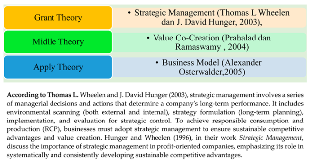
Efforts to achieve Responsible Consumption and Production (RCP) require strategic management within companies to ensure sustainable competitive advantage and value realization. Hunger and Wheelen (1996) discuss strategic management in their work "Strategic Management", explaining that applying strategic management in profit-oriented companies is essential for understanding competitive forces and systematically developing a sustainable competitive advantage.
Organic Agriculture and Sustainable Development. One of the agricultural systems that aligns with SDG 12: Responsible Consumption and Production is organic farming, which promotes sustainability. In Indonesia, organic farming has been expanding annually. The organic farming land area increased from 69,605.9 hectares in 2007 to 251,630.8 hectares in 2019, according to Organic Farming Statistics (SPOI, 2020). The global organic farming industry is also growing, with Indonesia ranking 21st worldwide. Based on demand data for organic products since 2019:
Jakarta leads with 32% of total consumption demand. West Java ranks second with 21% demand.Since the COVID-19 pandemic, demand for organic products has surged. Organic vegetables had the highest demand (20%) Organic fruits accounted for 11.59% There was also a growing demand for processed organic products (SPOI, 2020). The pandemic further influenced consumer habits: 27% consumed organic products daily, 10% consumed twice a day, 9.41% consumed every three days, 5.29% consumed weekly (AOI, 2020)., In terms of supply, organic products experiencing growth include:Organic coffee, tea, and rice (3.1%), Organic palm sugar (8–17 million tons) (Directorate of National Export Development, Ministry of Trade, 2020).Horticultural commodities such as bananas, oranges, and lettuce (SPOI, 2020).
Government Support for Organic Horticulture. Horticulture is a priority sector in Indonesian agriculture aimed at increasing national revenue. Government initiatives include: Expanding dryland horticulture outside Java. Constructing post-harvest storage facilities in production centers
Developing organic horticultural villages. Between 2012 and 2015, Indonesia's vegetable production area expanded from 1,033,817 hectares to 6,370,751 hectares (BPS, 2017), increasing national vegetable production and consumption opportunities (Apriyani et al., 2018). Supply chain efficiency is crucial for maintaining a steady supply, with continuity of supply being a key factor (Hadiguna & Marimin, 2007). However, data on comprehensive organic product supply, including processed and horticultural commodities, is still lacking (AOI).
Challenges in Organic Agriculture Development. According to Yosini Deliana et al. (2019), organic agriculture faces challenges related to: Market limitations – While global demand has risen, domestic demand remains weak. Consumers are primarily eco-conscious individuals willing to pay premium prices. Mislabeling – Some supermarkets label conventional products as organic without proper certification. Farmer participation – Many farmers lack knowledge or interest in organic farming. High certification costs – Organic certification is expensive. Weak farmer organizations – Small farmers struggle to establish agribusinesses without strong support. Weak partnerships – Collaboration between farmers and businesses remains ineffective. Marketing & promotion – Organic vegetable producers still struggle with digital marketing strategies. A key success factor in organic agriculture development is the farmer-business partnership, especially for export markets. Research on Value Co-Creation (VCC) with a Value Co-Design approach remains limited, particularly for organic vegetable products in domestic and export markets.
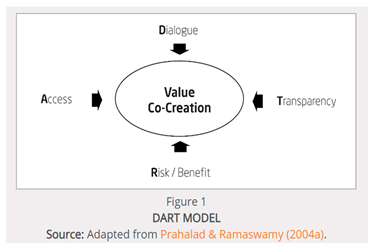
Value Co-Creation and Digital Marketing in Organic Agriculture. Service-Dominant Logic (SDL) in marketing suggests that customers play an active role in value creation through interactions with products and services (Vargo & Lusch, 2004). However, research has often overlooked individual consumer impact on Value Co-Creation (VCC) (Hoyer et al., 2010; Sugathan & Ranjan, 2019). Prahalad & Ramaswamy (2004) introduced the DART Model of Value Co-Creation, emphasizing: Dialogue, Access, Risk/Benefit Analysis,Transparency. Further research is needed to apply the DART model in social networks and sustainable community engagement. Digital platforms, including mobile applications, have been identified as effective tools for organic product marketing (Arogundade et al., 2020). With the rise of social media marketing, platforms like Facebook, Instagram, WhatsApp, Twitter, and websites have become crucial for B2C (Business-to-Customer) interactions in the Industry 4.0 and post-pandemic era (Fagerström & Ghinea, 2020).
The Shift Toward Healthy and Eco-Friendly Lifestyles. The COVID-19 pandemic accelerated a shift towards eco-friendly, chemical-free lifestyles. Consumers now prioritize safe, nutritious, and environmentally friendly food, increasing demand for organic vegetables globally (Mayrowani, 2012). However, organic vegetable consumption in Indonesia remains low, both domestically and for exports. Research suggests that digital platforms can enhance value creation, ultimately benefiting businesses (Feng Zhu, 2024).
The Role of Organic Farming Communities in Indonesia Indonesia’s organic farming sector consists of individuals, farmer groups, and private sector companies, many of which are members of AOI (Aliansi Organik Indonesia). Since 2002, AOI has had 147 members across 18 provinces, including: 43 NGOs, 26 Companies, 16 Farmer Organizations, 37 Individuals. Given the low awareness among consumers and producers regarding organic food, research is needed on Value Co-Creation (B2C) models for organic vegetables, effective digital platforms, and sustainable business models.
2. Baground
2.1. Novelty and Literature Review of VCC in Organic Vegetables
The indexed journal sources used for identification included Scopus, ScienceDirect, and Google Scholar. The initial identification of articles from these three sources, using the specified keywords, resulted in 52,395 articles. The screening process was then conducted based on relevant articles/topics and further refined using keyword C, narrowing the selection to 210 articles. Subsequently, an eligibility assessment was performed, including backward and forward review analysis, leading to a final total of 55 articles for review.

Table 1.
Keywords in Database Search and Number of Articles Found.
| Kode | Kata kunci | Scopus | ScienceDirect | G.Scholar | Jumlah |
|---|---|---|---|---|---|
| A | “value cocreation” | 5.795 | 700 | 44.900 | 52.395 |
| B | awareness* OR experience* OR knowledge* OR preference* | 521 | 53.024 | 397.000 | 450.545 |
| C | “colearning*” AND “coservice*” | 210 | 71 | 266 | 547 |
| D | “Consumption green product*” OR “organic product*” | 216 | 1.154 | 468 | 1.838 |
The review analysis method used is the PRISMA method (four-phase, flow-diagram) (Moher, Liberati et al., and Prisma Group, 2009; Vrabel, 2015), as explained in Figure 1. Based on the keyword search used in codes A, B, C, and D, the specific keywords were: A: ("value co-creation"), B: (knowledge* OR preference* OR awareness* OR experience*), C: ("co-learning" AND "co-service"), D: ("green product" OR "organic product").
Figure 2.
Value Co-Creation Publications Per Year in 2022 (Since 2014).
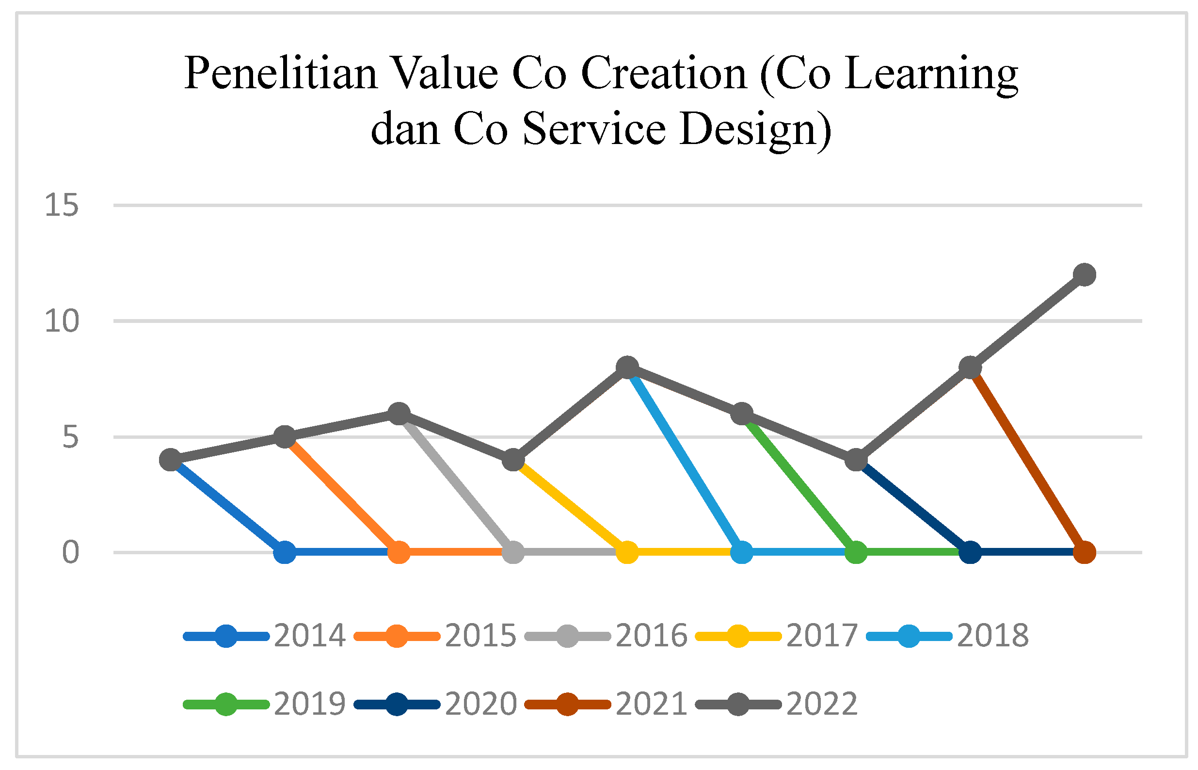
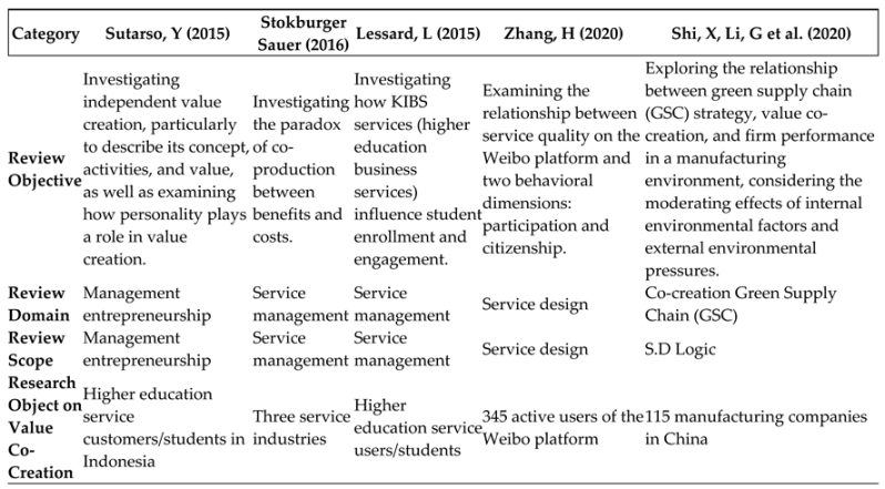
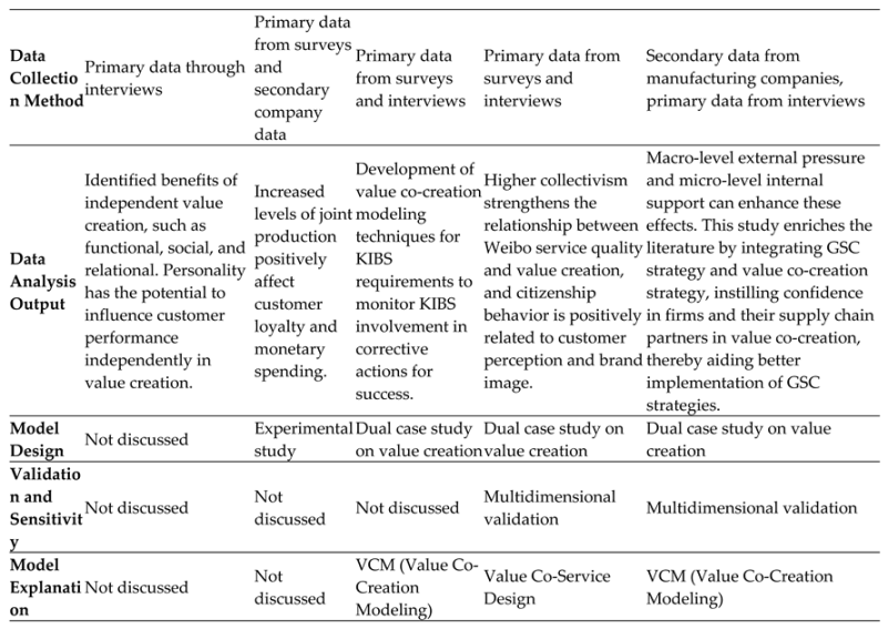
Table 2.
Summary of Discussions from Several Literature Reviews.
2.2. Research Novelty in Marketing Strategy with Value Co-Creation (Co-Learning and Co-Service Design)
The state of the art of this literature review lies in the application of value co-creation using the co-learning and co-service design approaches. These two approaches have been previously applied in KIBS (Knowledge-Intensive Business Services) and Miobi companies in China, where value co-creation was utilized for higher education service management and Miobi’s specialized online marketing applications. However, there has been no prior research on enhancing value to increase the consumption of local organic vegetables and exports to improve supply availability (MAK Siddike et al., 2014; K Komulainen, 2014; K Kimla, K Muto et al., 2015; GA Tangalah, R Jenal, Thahaya, 2021; LA Donovan et al., 2018; J Pocek et al., 2022; M Guseppe et al., 2022).
2.3. The Gap Between Marketing Strategy and the Research Topic of Value Co-Creation.
Figure 3.
Mapping of Bibliographic Value Co-Creation – Identified 8 Clusters.
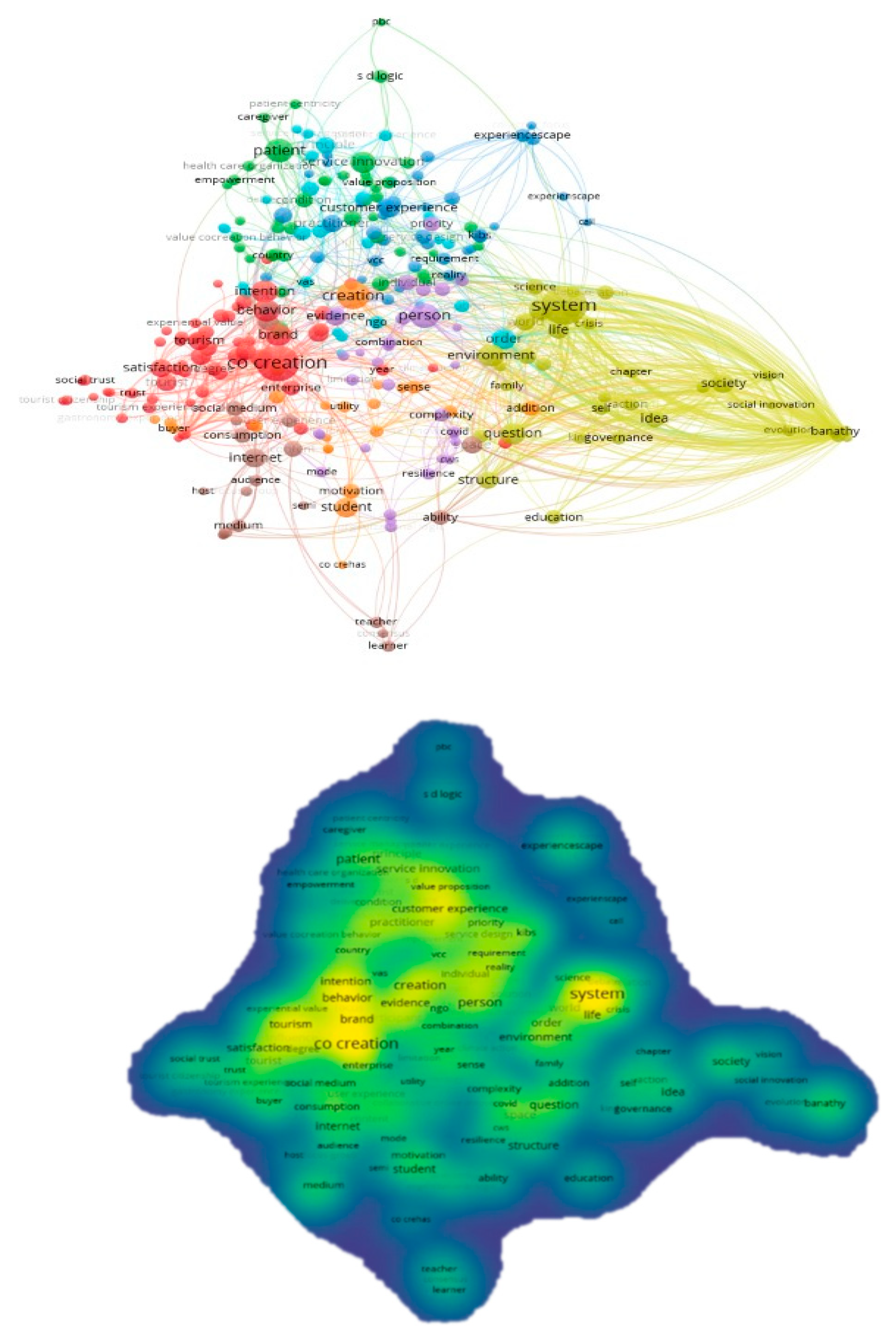
Table 3.
Top 10 Populer Keyword pada 8 Cluster Penelitian Value Co Creation.
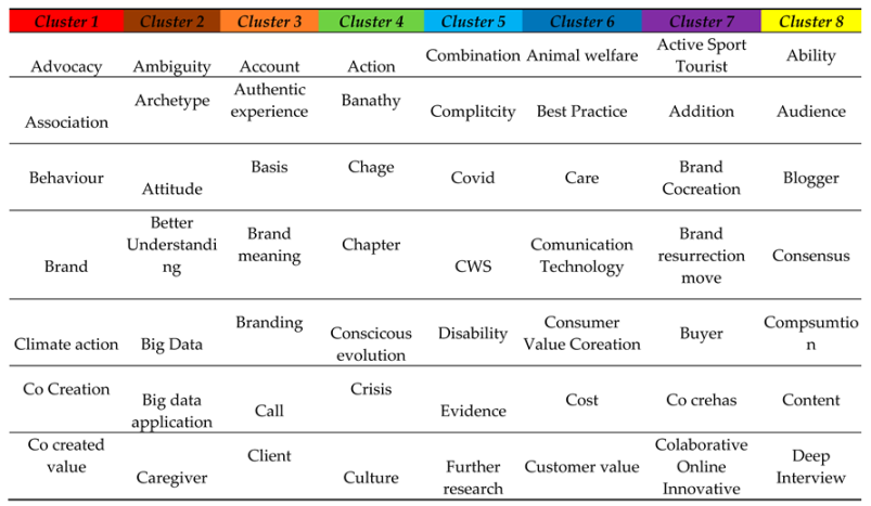
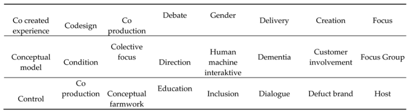
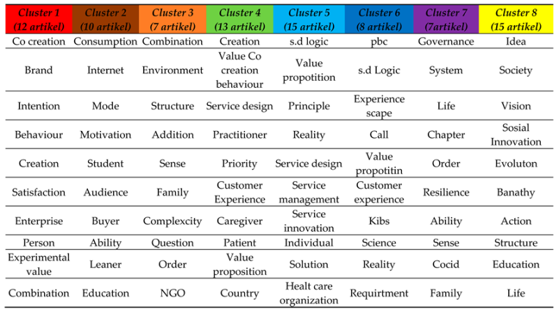
Table 4.
Top 10 Populer Keyword pada 8 Cluster Penelitian Value Co creation (Co learning dan Co service design).
Table 4.
Top 10 Populer Keyword pada 8 Cluster Penelitian Value Co creation (Co learning dan Co service design).
3. Methodology
Our Role as Academics and Members of Society in Managing Natural Resources for Sustainable Welfare
As academics and members of society, we must prioritize the responsible management of natural resources to ensure the welfare and prosperity of communities. Natural resource management should align with the mandate of the Creator—to utilize resources responsibly while maintaining the sustainability of humanity, preserving nature and the environment, and avoiding destruction or over-exploitation. Our role as both producers and consumers must uphold the objectives of the Sustainable Development Goals (SDGs). One of the key SDGs related to production and consumption is SDG 12: Responsible Consumption and Production (RCP). This goal emphasizes sustainable consumption and production practices. One commodity that has seen increasing demand, particularly after COVID-19, is vegetables, which are essential for boosting immunity. Given Indonesia’s tropical climate, various types of vegetables can be cultivated effectively. Most farmers in Indonesia use conventional, semi-organic, and organic farming systems. Organic vegetable farming aligns with SDG 12’s RCP objectives, as it ensures health safety and environmental sustainability by avoiding synthetic chemical fertilizers, pesticides, and artificial growth hormones. These natural farming practices enhance agricultural productivity while ensuring organic produce benefits consumers by supporting immune health.
- Challenges in the Organic Vegetable Market
The demand for organic vegetables is high, both locally and internationally, yet the supply from agricultural businesses remains low. Organic vegetable consumers primarily belong to communities that already understand the importance of consuming healthy food and contributing to environmental preservation. However, both internal and external business factors continue to present challenges in increasing public adoption of organic vegetable consumption. Consumers play a central role in providing valuable business data regarding their needs, preferences, and expectations. Businesses must analyze consumer data to improve services and enhance mutual value creation. By understanding factors affecting demand, supply, and preferred vegetable varieties (both locally and for export), businesses can enhance Value Co-Creation (VCC) to drive profitability. The information collected from the market can be categorized based on co-creation strategies to develop a robust business model for Business-to-Consumer (B2C) VCC in the organic vegetable sector.
Bridging the Gaps in Organic Vegetable Consumption Through Value Co-Creation (VCC)
Analysis of previous studies reveals certain limitations in their implications, particularly regarding psychological factors influencing the acceptance and consumption of organic vegetables. Besides product quality, promotion, and distribution, online marketing systems have also evolved significantly during the COVID-19 pandemic. Digital platforms and internet-based applications have become essential for consumers in obtaining healthy vegetables, presenting an opportunity for businesses to sustain their operations. However, many existing websites and e-commerce platforms still face challenges in their implementation, possibly due to inadequate marketing campaigns, lack of socialization, or insufficient consumer education. Many platforms fail to meet consumer expectations in terms of service and engagement. By leveraging an effective Value Co-Creation (VCC) model, this research aims to develop a B2C-based digital platform for organic vegetables, ensuring better understanding, acceptance, consumption levels, frequency, and consumer awareness. Furthermore, it aspires to cultivate influencers who actively promote responsible consumption and production (RCP) in the organic vegetable sector.
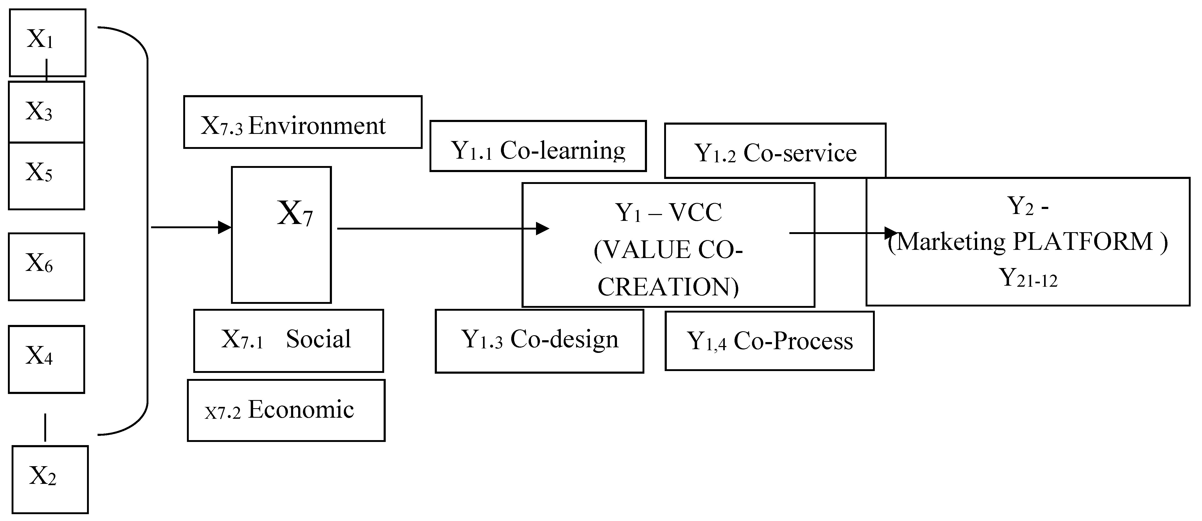
Figure 4.
Framework Diagram of VCC B2C Analysis for Organic Vegetables Using SEM LISREL.
-
Description:
- X1 = Demand and its indicators
- X2 = Supply and its indicators
- X3 = Dialogue
- X4 = Access
- X5 = Risk/Benefit
- X6 = Transparency
- X7 = Sustainability (economic, social, environmental)
- Y1 = Value Co-Creation (co-learning, co-design, co-process, co-service)
- Y2 = Online marketing platform (14 indicators)
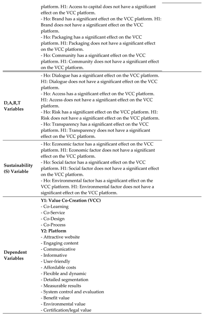
- Hypothesis Development
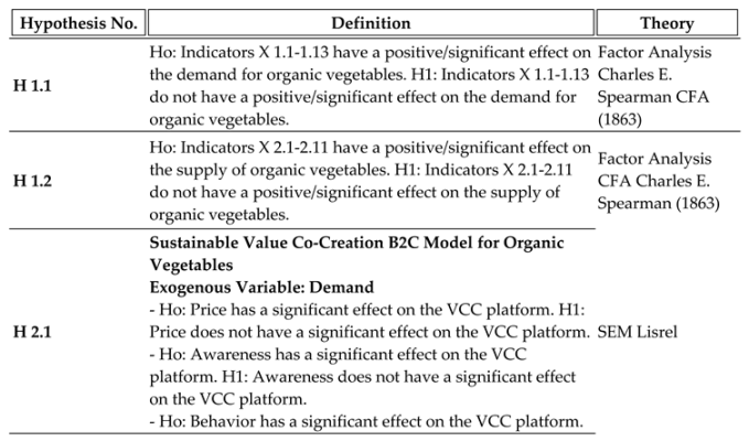
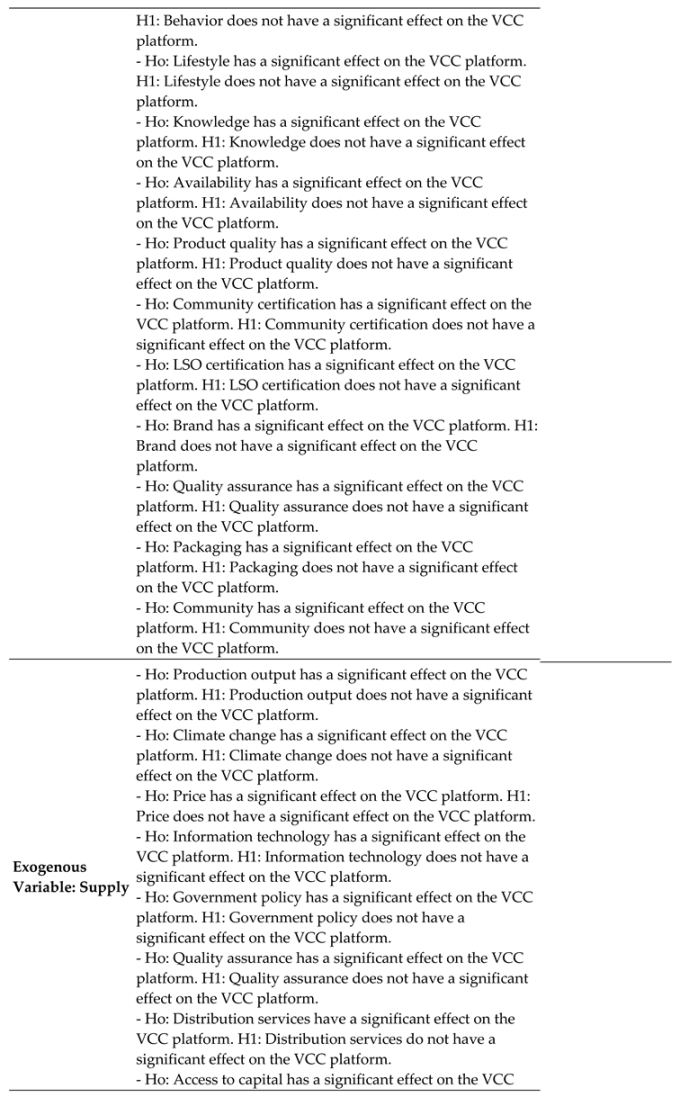
Table 5.
Research Hypotheses.
3.1. Research Method
The research was conducted in Indonesia, a location that serves as both a producer and consumer of organic and conventional vegetables, for the initial identification of organic vegetable business actors, business mentors, and a focus on West Java. The study specifically covered eight organic vegetable-producing regions: Sukabumi Regency, Cianjur Regency, Bogor, Depok, Bandung Regency, Garut Regency, Tasikmalaya Regency, and Ciamis Regency. The research was carried out from January 2023 to January 2024. The data collection technique used was purposive sampling, by selecting all business actors (organic vegetable producers) and mentors in West Java and 10 provinces (AOI data) as well as data from the Food and Horticulture Office. Additionally, random sampling was used to select 200 respondents consisting of organic and conventional vegetable consumers. The data sources consist of primary and secondary data. Primary data was obtained from questionnaires and direct interviews, product surveys, and focus group discussions (FGDs) involving and interview with google form for producers and consumers/communities of local and export organic vegetables, as well as non-organic consumers. Secondary data was sourced from organic horticulture businesses, AOI (Aliansi Organik Indonesia), relevant LSOs, IFOAM (International Federation of Organic Agriculture Movements), PAMOR (Organic Quality Assurance), export organic vegetable producers, stakeholders in export organic vegetable production, the West Java Food and Horticulture Office, the West Bandung Regency Agriculture Office, and the local Agricultural Extension Center (BPP).
3.2. Analyst Method
- A. Phase 1 Research:
The process of qualitative data collection is divided into two main categories: (1) Data collected by researchers through interviews, focus groups, or ethnographic field observations. (2) Pre-existing data in the form of documents before the study, such as public records, statistics, emails, etc.
For the second category, the data is already recorded, minimizing challenges in collection and management. Qualitative non-numeric data is obtained not only from primary data (interviews, focus group discussions (FGDs), and field observations) but also from secondary data, including: Written documentation and photographs, Researcher-recorded videos and YouTube videos, Content from various websites and WhatsApp, Discussions on social media platforms such as Twitter, LinkedIn, and Facebook, Non-numeric data from SPSS, Excel, and SurveyMonkey spreadsheets NVivo 11 Plus is used for visualizing data analysis results, including mind mapping, project mapping, and concept mapping. This tool is effective for content analysis, thematic analysis, and discourse analysis, The first phase of the research applies conditional analysis and participatory analysis (NVivo 11) and is validated using factor analysis.
- B. Factor Analysis Stages: (CFA Factor Analysis)
SPSS factor analysis is a method used to form factors in factor analysis using the SPSS application. Through this analysis, the following outcomes can be obtained:
- Identifying underlying dimensions or factors that explain the correlation among a set of variables.
- Identifying new, smaller variables to replace uncorrelated variables from a set of original variables that are correlated in multivariate analysis (such as regression analysis or discriminant analysis).
- Identifying key smaller variables that stand out from a larger set in a multivariate analysis.
- Steps:
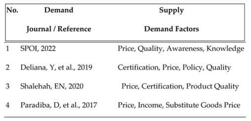
- Rate/rank the most frequently mentioned demand and supply factors from the research results, based on references and FGD (Focus Group Discussion) findings.
4. Result
4.1. Research Area Conditions
West Java, also known as Tatar Sunda, is a province in Indonesia. The capital of this province is Bandung City. In 2021, the population of West Java reached 48,782,408 people, with a density of 1,379 people/km². Based on the 2010 BPS census, West Java is the most populous province in Indonesia, with the indigenous population being the Sundanese ethnic group. West Java is located in the western part of Java Island. The province is bordered by Banten Province, DKI Jakarta Province, and the Java Sea to the north, Central Java Province to the east, the Indian Ocean to the south, and Banten Province and DKI Jakarta Province to the west. The northern coastal area consists of lowlands, while the central region is mountainous, forming part of the mountain range that extends from west to east across Java Island. The highest point in the province is Mount Ciremay, located southwest of Cirebon City. Several major rivers, such as the Citarum River and Cimanuk River, flow into the Java Sea.
West Java has a tropical climate, with the lowest recorded temperature reaching 9°C at the summit of Mount Pangrango, while the highest recorded temperature reaches 34°C in the northern coastal areas. The average annual rainfall across the province is approximately 2,000 mm, with some mountainous areas receiving 3,000 mm to 5,000 mm of rainfall per year. West Java consists of 18 regencies and 9 cities. The cities that have been newly established since 1996 are: West Java Province consists of 18 regencies, 9 municipalities, 627 districts, 645 sub-districts, and 5,312 villages. In 2017, the estimated population reached 44,039,313 people, with a total land area of 35,377.76 km².
West Java Province's Economic and Industrial Potential. West Java Province has a high concentration of manufacturing industries, including electronics, leather, food processing, textiles, furniture, and aircraft industries. Additionally, geothermal energy, oil and gas, and the petrochemical industry are among the province's key economic drivers. The largest contributor to West Java’s Gross Regional Domestic Product (GRDP) is the manufacturing sector (36.72%), followed by hospitality, trade, and agriculture (14.45%), bringing the total contribution to 51.17%. Despite economic crises, West Java remains the center of modern textile and garment industries in Indonesia, whereas other regions are more focused on traditional textile production. The province contributes nearly a quarter of Indonesia’s total non-oil and gas production value. Its main export commodity is textiles, accounting for 55.45% of West Java’s total exports. Additionally, West Java is one of the few provinces in Indonesia that exports iron ore, albeit in small quantities. The province is also home to industries such as steel production, footwear, furniture, rattan, electronics, and aircraft components.
Known as one of Indonesia’s "national rice barns", nearly 23% of its total area of 29,300 km² is dedicated to rice production. As Indonesia’s "Production Hub", West Java contributes 15% of Indonesia’s total agricultural output. The province produces rice, sweet potatoes, corn, fruits, and vegetables, as well as commodities like tea, coconut, palm oil, natural rubber, sugar, cocoa, and coffee. The livestock sector is also significant, with 120,000 cattle, representing 34% of the national total. West Java has two major coastal fronts: the Java Sea to the north and the Indian Ocean to the south, with a coastline spanning around 1,000 km. This geographical advantage provides immense potential for the fishing industry. The estimated fish catch potential in the southern coastal waters is 1.2 million tons per year, but the actual catch has only reached 11,000 tons per year. The total fish production in West Java is 1.6 million tons annually, with 280,000 to 300,000 tons (17.5% to 18.75%) coming from capture fisheries. This means that fish catches from the southern coast account for only 3.67% of West Java’s total capture fisheries production. A report from the West Java Marine and Fisheries Department (DKP) states that there are at least 120,000 fishermen in the province, along with an estimated millions of people engaged in aquaculture. West Java’s inland water resources are not only derived from its many rivers but also from water reservoirs such as Saguling Dam, Cirata Dam, and Jatiluhur Dam, which not only generate hydroelectric power but also support agricultural irrigation and freshwater fisheries.
As of 2003, West Java had a population of approximately 37 million people, accounting for 16% of Indonesia’s total population. Urbanization has been growing rapidly, particularly in the Greater Jakarta area (Jabodetabek). In 2001, West Java had 15.7 million educated workers, making up 18% of Indonesia’s total educated workforce. The majority of them were employed in agriculture, forestry, and fisheries (31%), followed by manufacturing (17%), trade, hospitality, and restaurants (22.5%), and services (29%).
Table 6.
Land Area and Organic Vegetable Production in Indonesia. West Java Ranks 3rd After Central Java and East Java.
Table 6.
Land Area and Organic Vegetable Production in Indonesia. West Java Ranks 3rd After Central Java and East Java.
| No | Province | 2019 | 2020 | 2021 | 2022 | ||||
| Land Area (ha) | Production (Ton) | Producers | Land Area (ha) | Production (Ton) | Producers | Land Area (ha) | Production (Ton) | ||
| 1 | DKI Jakarta | 8.4 | 4.2 | 0 | 20.15 | 10.075 | 0 | 20.15 | 10.075 |
| 2 | West Java | 147.53 | 865,257 | 117 | 138.8 | 928,397 | 131 | 140.87 | 1,091,040 |
| 3 | Central Java | 53.073 | 955,765 | 513 | 257.688 | 507,390 | 1,077 | 254.527 | 203,636 |
| 4 | Special Region of Yogyakarta | 2.305 | 94.48 | 17 | 2.105 | 166.1 | 12 | 1.78 | 140,942 |
| 5 | East Java | 80.588 | 1,828,439 | 237 | 75.087 | 639,362 | 306 | 42.357 | 1,188,106 |
Scheme 2022. Table 4.2 Respondent Characteristics 1.A. Mentors (2), Internal Data.
Table 7.
Respondent Mentors Characteristics.
| City/Regency | Number | Province | Number | Age (years) | Number | Education Level | Number |
| Sukabumi Regency | 4 | West Java | 4 | 25-35 | - | Elementary School | - |
| 36-46 | 3 | Junior High School | - | ||||
| 47-57 | 1 | Senior High School | - | ||||
| 58-70 | - | Higher Education | 4 | ||||
| Total | 4 | 4 | 4 | 4 | 4 | 4 | 4 |
| Cianjur Regency | 3 | West Java | 3 | 25-35 | - | Elementary School | - |
| 36-46 | 2 | Junior High School | - | ||||
| 47-57 | - | Senior High School | 1 | ||||
| 58-70 | - | Higher Education | 1 | ||||
| Total | 3 | 3 | 3 | 3 | 3 | 3 | 3 |
| Tasikmalaya Regency | 2 | West Java | 3 | 25-35 | 1 | Elementary School | - |
| 36-46 | 2 | Junior High School | - | ||||
| 47-57 | - | Senior High School | 2 | ||||
| 58-70 | - | Higher Education | 1 | ||||
| Total | 3 | 3 | 3 | 3 | 3 | 3 | 3 |
| Garut Regency | 3 | West Java | 3 | 25-35 | - | Elementary School | - |
| 36-46 | 3 | Junior High School | - | ||||
| 47-57 | - | Senior High School | 2 | ||||
| 58-70 | - | Higher Education | 1 | ||||
| Total | 3 | 3 | 3 | 3 | 3 | 3 | 3 |
| Bogor Regency | 2 | West Java | 2 | 25-35 | - | Elementary School | - |
| 36-46 | 1 | Junior High School | - | ||||
| 47-57 | 1 | Senior High School | - | ||||
| 58-70 | - | Higher Education | 2 | ||||
| Total | 2 | 2 | 2 | 2 | 2 | 2 | 2 |
| Depok | 2 | West Java | 2 | 25-35 | 1 | Elementary School | - |
| 36-46 | 1 | Junior High School | - | ||||
| 47-57 | - | Senior High School | - | ||||
| 58-70 | - | Higher Education | - | ||||
| Total | 2 | 2 | 2 | 2 | 2 | 2 | 2 |
| Bandung Barat Regency | 3 | West Java | 3 | 25-35 | 1 | Elementary School | - |
| 36-46 | 2 | Junior High School | - | ||||
| 47-57 | - | Senior High School | - | ||||
| 58-70 | - | Higher Education | 3 | ||||
| Total | 3 | 3 | 3 | 3 | 3 | 3 | 3 |
| Ciamis Regency | 4 | West Java | 4 | 25-35 | 3 | Elementary School | - |
| 36-46 | - | Junior High School | - | ||||
| 47-57 | 1 | Senior High School | 1 | ||||
| 58-70 | - | Higher Education | 3 | ||||
| Total | 4 | 4 | 4 | 4 | 4 | 4 | 4 |
| Total (West Java) | 23 | 23 | 23 | 23 | 23 | 23 | 23 |
| Outside West Java | 21 | 21 | 21 | 21 | 21 | 21 | 21 |
1.B. Mentors (20), Assisted Data.
Table 8.
Responden Mentor Characteristik.
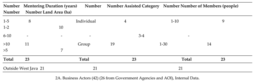
2A. Business Actors (42) (26 from Government Agencies and AOI), Internal Data.
Table 9.
Responden Business Actors Characteristic.
| City/Regency | Number | Province | Number | Age (years) | Number | Education Level | Number |
|---|---|---|---|---|---|---|---|
| Sukabumi Regency | 3 | West Java | 4 | 25-35 | - | Elementary School (SD) | - |
| - | - | - | 36-46 | 2 | Junior High School (SMP) | - | |
| - | - | - | 47-57 | 1 | Senior High School (SMA) | - | |
| - | - | - | 58-70 | - | Higher Education (PT) | 3 | |
| Total | 3 | 3 | 3 | 3 | 3 | 3 | 3 |
| Cianjur Regency | 6 | West Java | 6 | 25-35 | 2 | Elementary School (SD) | - |
| - | - | - | 36-46 | 2 | Junior High School (SMP) | - | |
| - | - | - | 47-57 | 2 | Senior High School (SMA) | 3 | |
| - | - | - | 58-70 | - | Higher Education (PT) | 3 | |
| Total | 6 | 6 | 6 | 6 | 6 | 6 | 6 |
| Tasikmalaya Regency | 5 | West Java | 5 | 25-35 | 1 | Elementary School (SD) | - |
| - | - | - | 36-46 | 2 | Junior High School (SMP) | - | |
| - | - | - | 47-57 | 2 | Senior High School (SMA) | 3 | |
| - | - | - | 58-70 | - | Higher Education (PT) | 2 | |
| Total | 5 | 5 | 5 | 5 | 5 | 5 | 5 |
| Bogor Regency | 6 | West Java | 6 | 25-35 | 2 | Elementary School (SD) | - |
| - | - | - | 36-46 | 2 | Junior High School (SMP) | - | |
| - | - | - | 47-57 | 1 | Senior High School (SMA) | 3 | |
| - | - | - | 58-70 | 1 | Higher Education (PT) | 3 | |
| Total | 6 | 6 | 6 | 6 | 6 | 6 | 6 |
| Depok | 5 | West Java | 5 | 25-35 | 2 | Elementary School (SD) | - |
| - | - | - | 36-46 | 1 | Junior High School (SMP) | - | |
| - | - | - | 47-57 | 2 | Senior High School (SMA) | 3 | |
| - | - | - | 58-70 | - | Higher Education (PT) | 2 | |
| Total | 5 | 5 | 5 | 5 | 5 | 5 | 5 |
| Garut Regency | 5 | West Java | 5 | 25-35 | 1 | Elementary School (SD) | - |
| - | - | - | 36-46 | 3 | Junior High School (SMP) | 1 | |
| - | - | - | 47-57 | - | Senior High School (SMA) | 2 | |
| - | - | - | 58-70 | 1 | Higher Education (PT) | 2 | |
| Total | 5 | 5 | 5 | 5 | 5 | 5 | 5 |
| West Bandung Regency | 6 | West Java | 6 | 25-35 | 2 | Elementary School (SD) | - |
| - | - | - | 36-46 | 3 | Junior High School (SMP) | - | |
| - | - | - | 47-57 | 1 | Senior High School (SMA) | 3 | |
| - | - | - | 58-70 | - | Higher Education (PT) | 3 | |
| Total | 6 | 6 | 6 | 6 | 6 | 6 | 6 |
| Ciamis Regency | 5 | West Java | 5 | 25-35 | 1 | Elementary School (SD) | - |
| - | - | - | 36-46 | 3 | Junior High School (SMP) | - | |
| - | - | - | 47-57 | 1 | Senior High School (SMA) | 2 | |
| - | - | - | 58-70 | - | Higher Education (PT) | 3 | |
| Total | 5 | 5 | 5 | 5 | 5 | 5 | 5 |
| Grand Total | 42 | 42 | 42 | 42 | 42 | 42 | 42 |
| Outside West Java | 21 | 21 | 21 | 21 | 21 | 21 | 21 |
2.B Business Actors, Business Capability Data.
Table 10.
Responden Business Actors Characteristic.
| Business Duration (years) | Number | Business Category | Number | Number of Members (people) | Number | Land Area (ha) | Number | Vegetable Production (tons) | Number | Revenue (Rp/month) | Number |
| 1-5 | 12 | Individual | 7 | 1-10 | 5 | 1-2 | 14 | 0.25-0.5 | 25 | <5,000,000 | 15 |
| 6-10 | |||||||||||
| >10 | 15 | Group | 35 | 1-30 | 37 | 3-4 | >0.5 | 20 | >5,000,000 | 27 | |
| Total | 42 | 42 | 42 | 42 | 42 | 42 |
Table 11.
Open-Ended Question Data.
| Region | Local Vegetable Types | Export Vegetable Types | Largest Demand Areas | Domestic VCC Needs | Export VCC Needs | Marketing Channels | Value of Collaboration in Community |
| West Java | Pakcoy, mustard greens, spinach | Horenzo, pakcoy, lettuce | Bogor, Cipanas, Bandung, Jakarta | Marketing innovation, services, pricing, products | Quality, policies, distribution system | Online, organic circle, modern market | Price standards, sustainability, standardization |
| Outside West Java | Broccoli, spinach, water spinach | Lettuce | Prigen, Batu Malang, Central Java | Product innovation, marketing | Policies, quality |
3.Consumers of Organic and Conventional Vegetables (135 People).
Table 12.
Responden Consumers Characteristic.
| City/Regency | Number | Province | Number | Age (years) | Number | Education Level | Number |
| Sukabumi Regency | 10 | West Java | 10 | 25-35 | 7 | Elementary School (SD) | - |
| - | - | - | 36-46 | 3 | Junior High School (SMP) | - | |
| - | - | - | 47-57 | - | Senior High School (SMA) | - | |
| - | - | - | 58-70 | - | Higher Education (PT) | 10 | |
| Total | 10 | 10 | 10 | 10 | 10 | 10 | 10 |
| Cianjur Regency | 15 | West Java | 15 | 25-35 | 5 | Elementary School (SD) | - |
| - | - | - | 36-46 | 8 | Junior High School (SMP) | - | |
| - | - | - | 47-57 | 2 | Senior High School (SMA) | 10 | |
| - | - | - | 58-70 | - | Higher Education (PT) | 5 | |
| Total | 15 | 15 | 15 | 15 | 15 | 15 | 15 |
| Tasikmalaya Regency | 15 | West Java | 15 | 25-35 | 8 | Elementary School (SD) | - |
| - | - | - | 36-46 | 5 | Junior High School (SMP) | - | |
| - | - | - | 47-57 | 2 | Senior High School (SMA) | 8 | |
| - | - | - | 58-70 | - | Higher Education (PT) | 7 | |
| Total | 15 | 15 | 15 | 15 | 15 | 15 | 15 |
| Bogor Regency | 20 | West Java | 20 | 25-35 | 5 | Elementary School (SD) | - |
| - | - | - | 36-46 | 7 | Junior High School (SMP) | - | |
| - | - | - | 47-57 | 5 | Senior High School (SMA) | 10 | |
| - | - | - | 58-70 | 3 | Higher Education (PT) | 10 | |
| Total | 20 | 20 | 20 | 20 | 20 | 20 | 20 |
| Depok | 25 | West Java | 25 | 25-35 | 5 | Elementary School (SD) | - |
| - | - | - | 36-46 | 8 | Junior High School (SMP) | - | |
| - | - | - | 47-57 | 7 | Senior High School (SMA) | 12 | |
| - | - | - | 58-70 | 5 | Higher Education (PT) | 13 | |
| Total | 25 | 25 | 25 | 25 | 25 | 25 | 25 |
| Garut Regency | 15 | West Java | 15 | 25-35 | 4 | Elementary School (SD) | - |
| - | - | - | 36-46 | 6 | Junior High School (SMP) | 2 | |
| - | - | - | 47-57 | 1 | Senior High School (SMA) | 8 | |
| - | - | - | 58-70 | 4 | Higher Education (PT) | 5 | |
| Total | 15 | 15 | 15 | 15 | 15 | 15 | 15 |
| West Bandung Regency | 25 | West Java | 25 | 25-35 | 5 | Elementary School (SD) | - |
| - | - | - | 36-46 | 8 | Junior High School (SMP) | - | |
| - | - | - | 47-57 | 7 | Senior High School (SMA) | 3 | |
| - | - | - | 58-70 | 5 | Higher Education (PT) | 3 | |
| Total | 25 | 25 | 25 | 25 | 25 | 25 | 25 |
| Ciamis Regency | 10 | West Java | 10 | 25-35 | 4 | Elementary School (SD) | - |
| - | - | - | 36-46 | 3 | Junior High School (SMP) | - | |
| - | - | - | 47-57 | 3 | Senior High School (SMA) | 4 | |
| - | - | - | 58-70 | - | Higher Education (PT) | 6 | |
| Total | 10 | 10 | 10 | 10 | 10 | 10 | 10 |
| Total | 135 | 135 | 135 | 135 | 135 | 135 | 135 |
| Outside West Java | 33 | 33 | 33 | 33 | 33 | 33 | 33 |
Table 13.
Respondent Characteristics of Organic and Conventional Vegetables (200 respondents, internal data).
Table 13.
Respondent Characteristics of Organic and Conventional Vegetables (200 respondents, internal data).
| Region | Income (IDR) | Number | % | Age (years) | Number | % | Education Level | Number | % |
| West Java | < 2,000,000 | 30 | 15 | 25-35 | 66 | 33 | Elementary School (SD) | - | - |
| 2.5 – 4,000,000 | 57 | 28.5 | 36-46 | 75 | 37.5 | Junior High School (SMP) | 3 | 1.5 | |
| 4.0 – 7,000,000 | 78 | 39 | 47-57 | 40 | 20 | Senior High School (SMA) | 106 | 53 | |
| > 7,500,000 | 35 | 17.5 | 58-70 | 19 | 9.5 | Higher Education (PT) | 91 | 45.4 | |
| Total | 200 | 100 | 200 | 100 | 200 | 100 |
Table 14.
Organic Vegetable Consumption and Online Purchase Behavior.
| Region | Consumes/Purchases Organic Vegetables | Number | % | Aware of Organic Vegetable Platforms | Number | % | Buys Organic Vegetables Online | Number | % |
| West Java | Yes | 179 | 89.5 | Lingkar Organik | 63 | 31.5 | Sometimes | 71 | 35.5 |
| No | 18 | 9 | Kecipir | 49 | 24.5 | Ever | 45 | 22.5 | |
| Sometimes | 3 | 1.5 | edas | 57 | 28.5 | Never | 84 | 42 | |
| Sesa.id | 33 | 16.5 | |||||||
| Total | 200 | 100 | 200 | 100 | 200 | 100 |
4.2. Factor Analysis Results (Identification of Problem 1) - CFA
4.2.1. Demand Factor Analysis
Analysis of the Most Determining Factors for Organic Vegetable Demand
Goodness of Fit Test for the Factor Analysis Model Affecting Organic Vegetable Demand
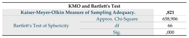
Kaiser-Meyer-Olkin (KMO) and Bartlett’s Test
The Kaiser-Meyer-Olkin (KMO) test is used as an initial test to determine whether the available data can be broken down into a set of factors (Santoso, 2015). The KMO test is also utilized to assess the model fit or goodness of fit of the factor analysis model for the demand of organic vegetables, using the chi-square statistical test. Factor analysis model criteria:
- If the p-value or significance level (sig) is < 0.05, then the factor analysis model is fit or good.
- If the p-value or significance level (sig) is > 0.05, then the factor analysis model is not fit or not good, and data transformation is required.
The results of the KMO and Bartlett’s Test in Table 1 indicate that the KMO value for the factor analysis model affecting the demand for local and export organic vegetables is 0.821. The Bartlett’s Test produced a Chi-Square value of 658.91, with a significance value (sig) of 0.000, which is well below 0.05 (0.00 < 0.05). This means that the available variables and samples are suitable for factor analysis.Therefore, the factor analysis model for the demand for local and export organic vegetables is appropriate, allowing further analysis, including Factor Extraction and Rotation.
Table 15.
KMO Measurement Results and Bartlett’s Test.
Analysis of Eigenvalues, Factor Extraction, and Rotation
After conducting the goodness of fit test and confirming that the factor analysis model influencing the demand for local and export organic vegetables is valid, the next step is to perform an analysis of eigenvalues, factor extraction, and rotation.
Eigenvalues indicate the relative importance of each factor in explaining the variance of all analyzed variables. This study examines 12 variables suspected to influence the demand for local and export organic vegetables: Awareness (X1), Behavior (X2), Lifestyle (X3), Knowledge (X4), Availability (X5), Price (X6), Trust in Product (X7), Quality Assurance (X8), Community Certification (X9), LSO Certification (X10), Innovation Value (X11), and Product Quality (X12). The eigenvalues show the relative importance of each factor in explaining the variance among these 12 variables.
Based on Table 2, only three factors are formed. With one factor, the eigenvalue is above 1. With two factors, the eigenvalue remains above 1. With three factors, the eigenvalue is still above 1 (1.102). However, for four factors, the eigenvalue falls below 1 (0.980), meaning the factoring process must stop at three factors.
Thus, based on the eigenvalue analysis, it can be concluded that from the 12 analyzed variables, the demand for local and export organic vegetables can be summarized into only three main influencing factors.
Table 16.
Results of Eigenvalues, Factor Extraction, and Rotation.
Factor Loading and Validity Test of the Factor Analysis Model Influencing the Demand for Local and Export Organic Vegetables
The Component Matrix from the rotation process (Rotated Component Matrix) is presented in Table 3. This table clearly shows the final distribution of variables in the factor analysis. Each variable is assigned to a factor where it has the highest factor loading value, which must be at least 0.5 or less than -0.5. If a variable does not reach a factor loading of ±0.5 for any of the three factors, it is considered invalid.
Table 17.
Rotated Component Matrix: Factor Loading Values of 12 Variables for the Three Formed Components.
Table 17.
Rotated Component Matrix: Factor Loading Values of 12 Variables for the Three Formed Components.
Based on Table 3, out of the 12 variables, one variable was found to be invalid, namely X11 (Innovation Value). The remaining 11 variables have been successfully reduced into three factors, as follows:
- Factor 1 consists of Awareness (X1), Behavior (X2), Lifestyle (X3), Knowledge (X4), and Trust in Product (X7).
- Factor 2 consists of Price (X6), Quality Assurance (X8), Community Certification (X9), and LSO Certification (X10).
- Factor 3 consists of Availability (X5) and Product Quality (X12).
Naming the Factors
-
Factor 1: Consumer Internal FactorsSince all five variables in Factor 1 have positive factor loading values, this factor can be named Consumer Internal Factors. This means that the increasing demand for local and export organic vegetables is influenced by consumer awareness of the importance of organic vegetable consumption, healthier consumer behavior, a healthier lifestyle, greater consumer knowledge of healthy living, and higher trust in organic vegetable products.
-
Factor 2: Product Exclusivity FactorsSince all four variables in Factor 2 also have positive factor loading values, this factor can be named Product Exclusivity Factors. This indicates that the higher demand for local and export organic vegetables is driven by higher product prices, clearer quality assurance, the presence of local and international organic community certifications, and LSO certification.
-
Factor 3: Strength FactorsSince Availability (X5) has a positive factor loading value, this suggests that the increased availability of organic vegetables in the market contributes to higher demand. However, Product Quality (X12) has a negative factor loading value, indicating that as demand for organic vegetables increases, product quality tends to decrease. This may be due to consumer perception that if vegetables appear too perfect, they might have been treated with chemical pesticides, making them less desirable compared to conventional vegetables.
4.2.2. Factor Analysis of Supply
Analysis of the Key Factors Determining the Supply of Organic Vegetables
1. Goodness of Fit Test for the Factor Analysis Model Affecting the Supply of Local and Export Organic Vegetables
1.1 Kaiser-Meyer-Olkin (KMO) and Bartlett’s Test
The Kaiser-Meyer-Olkin (KMO) test is used as a preliminary test to determine whether the available data can be broken down into a number of factors (Santoso, 2015). The KMO test is also used to assess the goodness of fit of the factor analysis model for formal and informal sector rice seed using chi-square statistical testing.
The criteria for factor analysis modeling are as follows:
- If the p-value (significance level) is less than 0.05, the factor analysis model is considered fit or good.
- If the p-value (significance level) is greater than 0.05, the factor analysis model is considered not fit or not good, and data transformation is required.
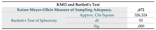
The KMO and Bartlett’s Test results in Table 1 show that the KMO value for the factor analysis model affecting the supply of local and export organic vegetables is 0.672. Additionally, the Bartlett’s Test result shows a Chi-Square value of 326.32 with a significance level (sig) of 0.000, which is well below 0.05 (0.00 < 0.05). This indicates that the variables and sample used are suitable for factor analysis.
Therefore, the factor analysis model for the supply of local and export organic vegetables is valid, allowing for further analysis, including Factor Extraction and Rotation.
Table 18.
KMO and Bartlett’s Test Results.
Eigenvalues Analysis, Factor Extraction, and Rotation
After conducting the goodness of fit test and confirming that the factor analysis model influencing the supply of local organic vegetables is valid, the next step involves Eigenvalues analysis, factor extraction, and factor rotation.
Eigenvalues represent the relative importance of each factor in explaining the variance of all analyzed variables. In this study, 11 variables were examined for their potential impact on the supply organic vegetables, including:Production output (X1), Climate change (X2), Government policy for the domestic market (X3), Government policy for the export market (X4), Quality assurance (X5), Information technology (X6), Capital access (X8), Brand (X9), Packaging (X10), Community (X11). Eigenvalues indicate the relative importance of each factor in calculating the variance of these 11 analyzed variables.
Based on Table 2, only three factors were identified:
- With one factor, the eigenvalue remains above 1.
- With two factors, the eigenvalues are still above 1.
- With three factors, the eigenvalue remains above 1, specifically 1.296.
- However, with four factors, the eigenvalue drops below 1 (0.977), meaning that the factoring process must stop at three factors.
Thus, based on the Eigenvalues analysis, it can be concluded that the 11 analyzed variables can be summarized into three main factors that influence the supply organic vegetables.
Table 19.
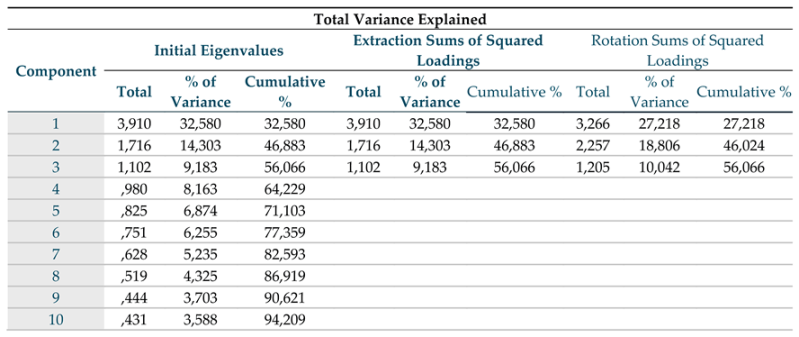
Eigenvalues, Factor Extraction, and Rotation Results.
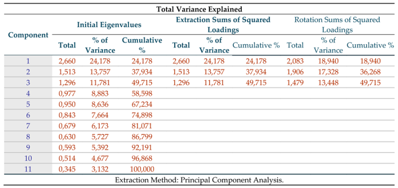
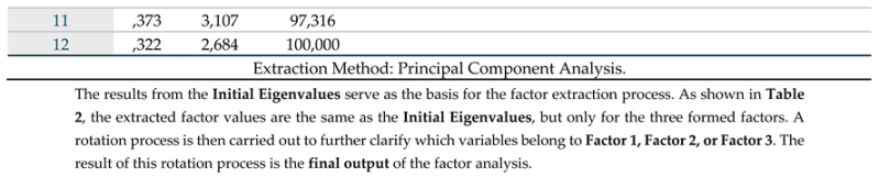
Factor Extraction and Rotation Process
The results from the Initial Eigenvalues serve as the foundation for the factor extraction process. The extracted factors, as shown in Table 2, retain the same values as the Initial Eigenvalues but only for the three identified factors. Next, the rotation process is applied to enhance clarity in categorizing variables into Factor 1, Factor 2, or Factor 3. The final output of this rotation process represents the conclusive results of the factor analysis.
2. Factor Loading and Validity Test of the Factor Analysis Model for Organic Vegetable Supply
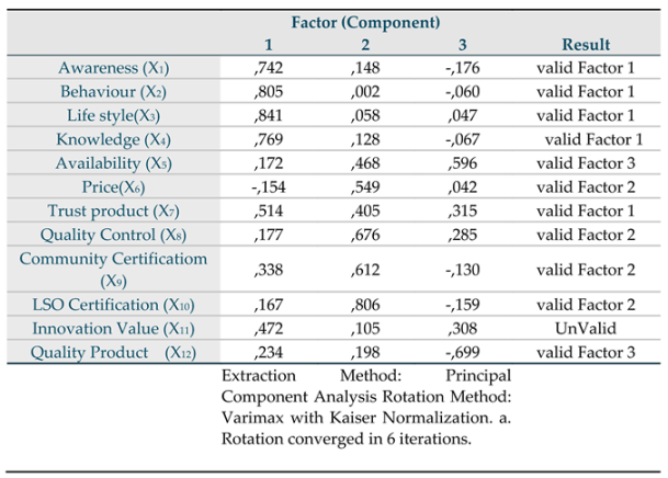
The Component Matrix obtained after the rotation process (Rotated Component Matrix), presented in Table 3, provides a clearer and more structured distribution of variables in the factor analysis. Each variable is assigned to the factor where it has the highest factor loading value, with a minimum threshold of 0.5 or a negative value lower than -0.5. If a variable fails to reach a factor loading value of ±0.5 for any of the three factors, it is considered invalid.
Table 20.
Rotated Component Matrix: Factor Loading Values of 11 Variables in the Three Identified Factors.
Table 20.
Rotated Component Matrix: Factor Loading Values of 11 Variables in the Three Identified Factors.
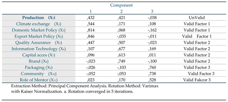
Based on Table 3, out of the 11 variables, one variable is invalid, namely variable X1 (production output). Meanwhile, the remaining 10 variables have been successfully reduced into three factors:
- Factor 1 consists of Climate Change (X2), Government Policy – Domestic Market (X3), and Government Policy – Export Market (X4).
- Factor 2 consists of Quality Assurance (X5), Information Technology (X6), Capital Access (X7), and Brand (X8).
- Factor 3 consists of Packaging (X9), Community (X10), and Role of Mentors (X11).
Factor 1: Key Supporting Factor
Factor 1 includes Climate Change (X2), Government Policy – Domestic Market (X3), and Government Policy – Export Market (X4). If named, this factor can be called the Key Supporting Factor. Since the factor loadings of these three variables are positive, this means that the increasing supply of local and export organic vegetables is influenced by the Key Supporting Factor, characterized by more stable climate conditions, government policies that support the growth of the domestic market, and policies that promote export market expansion. (Further discussion can be added here.)
Factor 2: Exclusive Factor
Factor 2 includes Quality Assurance (X5), Information Technology (X6), Capital Access (X7), and Brand (X8). If named, this factor can be called the Exclusive Factor. The positive factor loadings of these four variables indicate that the increasing supply of local and export organic vegetables is influenced by the Exclusive Factor, marked by better quality assurance, easier access to capital for farmers, improved farmer skills in utilizing information technology, and greater brand recognition of organic vegetable products. (Further discussion can be added here.)
Factor 3: Strengthening Support Factor
Factor 3 includes Packaging (X9), Community (X10), and Role of Mentors (X11). If named, this factor can be called the Strengthening Support Factor. The positive factor loadings of these three variables indicate that the increasing supply of local and export organic vegetables is influenced by the Strengthening Support Factor, characterized by improved product packaging, a supportive organic farming community, and a better role of mentors in enhancing organic vegetable production. (Further discussion can be added here.)
VCC B2C Model for Organic Vegetables (Development of the DART Model)
Multivariate Outlier Test
The multivariate outlier examination was conducted using the Mahalanobis Distance (d²) statistic by testing the following hypotheses:
- H₀: The data does not contain multivariate outliers.
- H₁: The data contains multivariate outliers.
The decision criterion is to reject H₀ for any row of data if the Mahalanobis Distance (d²) exceeds the chi-square value χ²(p<0.001; k), where k is the number of manifest variables (indicators).
The test results indicate that in this Structural Equation Modeling (SEM) model, k = 47 indicators or manifest variables, yielding a chi-square value of χ²(p<0.001;47) = 82.72. Among the total 200 data points, 5 data points have Mahalanobis Distance (d²) values greater than the chi-square threshold of 82.72 (Table 1). As a result, H₀ is rejected for these data points, meaning that they contain multivariate outliers and must be removed from the analysis.
Meanwhile, the remaining data points have Mahalanobis Distance values below the chi-square threshold, indicating that they do not contain multivariate outliers. Consequently, the final dataset for further analysis consists of 195 respondent data points. A complete report of this test is provided in Appendix 1.
Table 21.
List of Data Containing Multivariate Outliers.
| No. | Mahalanobis Distance (d²) | Chi-square Value χ²(p<0.001;47) | Status |
| 134 | 86.60316 | 82.72042 | Outlier |
| 136 | 198.005 | 82.72042 | Outlier |
| 137 | 198.005 | 82.72042 | Outlier |
| 138 | 198.005 | 82.72042 | Outlier |
| 161 | 82.85639 | 82.72042 | Outlier |
Multivariate Normality Test
The results of the normality test are shown in the following table (the complete results can be found in Appendix 2).
Table 22.
Results of Univariate and Multivariate Normality Test.
| Variabel Manifest | Univariate Normality | Multivariate Normality | ||
| Skewness and Kurtosis | Skewness and Kurtosis | |||
| Chi-Square | P-Value | Chi-Square | P-Value | |
| X5 | 0.210 | 0.900 | 335.377 | 0.000 |
| X3 | 1.613 | 0.446 | ||
| X1-1 | 1.044 | 0.593 | ||
| X1-2 | 0.119 | 0.942 | ||
| X1-3 | 1.553 | 0.460 | ||
| X1-4 | 3.044 | 0.218 | ||
| X1-5 | 5.485 | 0.064 | ||
| X1-6 | 1.255 | 0.534 | ||
| X1-7 | 1.098 | 0.578 | ||
| X1-8 | 0.701 | 0.704 | ||
| X1-9 | 3.755 | 0.153 | ||
| X1-10 | 0.738 | 0.691 | ||
| X1-11 | 1.719 | 0.423 | ||
| X1-12 | 2.569 | 0.277 | ||
| X2-1 | 1.985 | 0.371 | ||
| X2-2 | 4.192 | 0.123 | ||
| X2-3 | 4.739 | 0.094 | ||
| X2-4 | 4.646 | 0.098 | ||
| X2-5 | 0.680 | 0.712 | ||
| X2-6 | 0.931 | 0.628 | ||
| X2-7 | 7.225 | 0.054 | ||
| X2-8 | 0.754 | 0.686 | ||
| X2-9 | 2.405 | 0.300 | ||
| X2-10 | 3.973 | 0.137 | ||
| X2-11 | 0.754 | 0.686 | ||
| X4 | 2.404 | 0.301 | ||
| X6 | 1.274 | 0.529 | ||
| Y1-1 | 0.627 | 0.731 | ||
| Y1-2 | 0.444 | 0.801 | ||
| Y1-3 | 0.005 | 0.997 | ||
| Y1-4 | 0.675 | 0.714 | ||
| X7-1 | 5.572 | 0.062 | ||
| X7-2 | 0.058 | 0.971 | ||
| X7-3 | 0.043 | 0.979 | ||
| Y2-1 | 3.044 | 0.218 | ||
| Y2-2 | 2.458 | 0.293 | ||
| Y2-3 | 1.104 | 0.576 | ||
| Y2-4 | 0.743 | 0.690 | ||
| Y2-5 | 1.862 | 0.394 | ||
| Y2-6 | 0.650 | 0.723 | ||
| Y2-7 | 2.705 | 0.259 | ||
| Y2-8 | 5.699 | 0.058 | ||
| Y2-9 | 0.062 | 0.970 | ||
| Y2-10 | 1.568 | 0.457 | ||
| Y2-11 | 1.230 | 0.541 | ||
| Y2-12 | 0.889 | 0.641 | ||
| Y2-13 | 0.682 | 0.711 | ||
Based on the table above, the results of the normality test for each variable (univariate normality) show that all manifest variables have p-values for Skewness and Kurtosis greater than 0.05. This indicates that none of the manifest variables have issues with univariate normality, meaning they can all be included in the next stage of analysis since the normality assumption, which is a fundamental requirement for SEM analysis, has been met. Meanwhile, the normality test results for all variables combined (multivariate normality) indicate that the multivariate normality assumption has not been met, as the p-value for Skewness and Kurtosis is 0.000, which is still less than 0.05. This means the data still faces normality issues at the multivariate level.
In principle, if the univariate normality assumption is fulfilled, the indicators can be considered normal. However, to address the issue of multivariate normality violations, adjustments will be made in the model estimation process by applying the Satorra-Bentler Scaled χ² method. This involves incorporating the asymptotic covariance matrix input in addition to the data covariance matrix input, which will generate a Goodness of Fit value to correct for data non-normality (Yamin, 2014). Therefore, the analysis will proceed with the manifest variables that have met the univariate normality assumption.
Multicollinearity Test
The results of the multicollinearity test are shown in the table below (the complete results can be found in Appendix 3).
Table 23.
Multicollinearity Test Results.
| Variabel Manifest | Collinearity Statistics | Result | |
| Tolerance | VIF | ||
| X5 | ,425 | 2,354 | Unmultikolinieritas |
| X3 | ,325 | 3,073 | Unmultikolinieritas |
| X1-1 | ,471 | 2,124 | Unmultikolinieritas |
| X1-2 | ,446 | 2,242 | Unmultikolinieritas |
| X1-3 | ,369 | 2,711 | Unmultikolinieritas |
| X1-4 | ,416 | 2,405 | Unmultikolinieritas |
| X1-5 | ,632 | 1,582 | Unmultikolinieritas |
| X1-6 | ,673 | 1,485 | Unmultikolinieritas |
| X1-7 | ,556 | 1,799 | Unmultikolinieritas |
| X1-8 | ,553 | 1,809 | Unmultikolinieritas |
| X1-9 | ,558 | 1,791 | Unmultikolinieritas |
| X1-10 | ,490 | 2,043 | Unmultikolinieritas |
| X1-11 | ,662 | 1,510 | Unmultikolinieritas |
| X1-12 | ,804 | 1,244 | Unmultikolinieritas |
| X2-1 | ,681 | 1,469 | Unmultikolinieritas |
| X2-2 | ,680 | 1,470 | Unmultikolinieritas |
| X2-3 | ,515 | 1,943 | Unmultikolinieritas |
| X2-4 | ,492 | 2,033 | Unmultikolinieritas |
| X2-5 | ,604 | 1,655 | Unmultikolinieritas |
| X2-6 | ,605 | 1,653 | Unmultikolinieritas |
| X2-7 | ,699 | 1,431 | Unmultikolinieritas |
| X2-8 | ,670 | 1,493 | Unmultikolinieritas |
| X2-9 | ,747 | 1,339 | Unmultikolinieritas |
| X2-10 | ,729 | 1,373 | Unmultikolinieritas |
| X2-11 | ,776 | 1,289 | Unmultikolinieritas |
| X4 | ,369 | 2,710 | Unmultikolinieritas |
| X6 | ,517 | 1,934 | Unmultikolinieritas |
| Y1-1 | ,617 | 1,621 | Unmultikolinieritas |
| Y1-2 | ,223 | 4,494 | Unmultikolinieritas |
| Y1-3 | ,423 | 2,367 | Unmultikolinieritas |
| Y1-4 | ,422 | 2,372 | Unmultikolinieritas |
| X7-1 | ,223 | 4,475 | Unmultikolinieritas |
| X7-2 | ,323 | 3,092 | Unmultikolinieritas |
| X7-3 | ,523 | 1,910 | Unmultikolinieritas |
| Y2-1 | ,380 | 2,633 | Unmultikolinieritas |
| Y2-2 | ,480 | 2,084 | Unmultikolinieritas |
| Y2-3 | ,216 | 4,637 | Unmultikolinieritas |
| Y2-4 | ,520 | 1,922 | Unmultikolinieritas |
| Y2-5 | ,148 | 6,764 | Unmultikolinieritas |
| Y2-6 | ,383 | 2,613 | Unmultikolinieritas |
| Y2-7 | ,648 | 1,544 | Unmultikolinieritas |
| Y2-8 | ,283 | 3,537 | Unmultikolinieritas |
| Y2-9 | ,434 | 2,303 | Unmultikolinieritas |
| Y2-10 | ,198 | 5,045 | Unmultikolinieritas |
| Y2-11 | ,598 | 1,672 | Unmultikolinieritas |
| Y2-12 | ,423 | 2,363 | Unmultikolinieritas |
| Y2-13 | ,524 | 1,908 | Unmultikolinieritas |
The results of the multicollinearity test indicate that the tolerance values for all manifest variables are within an acceptable range. This is evidenced by the VIF values for all manifest variables, none of which exceed 5. Therefore, it can be concluded that there is no excessively high correlation between any manifest variable/indicator and another. As a result, all manifest variables/indicators are free from multicollinearity, allowing them to proceed to the next stage of testing
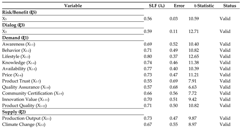
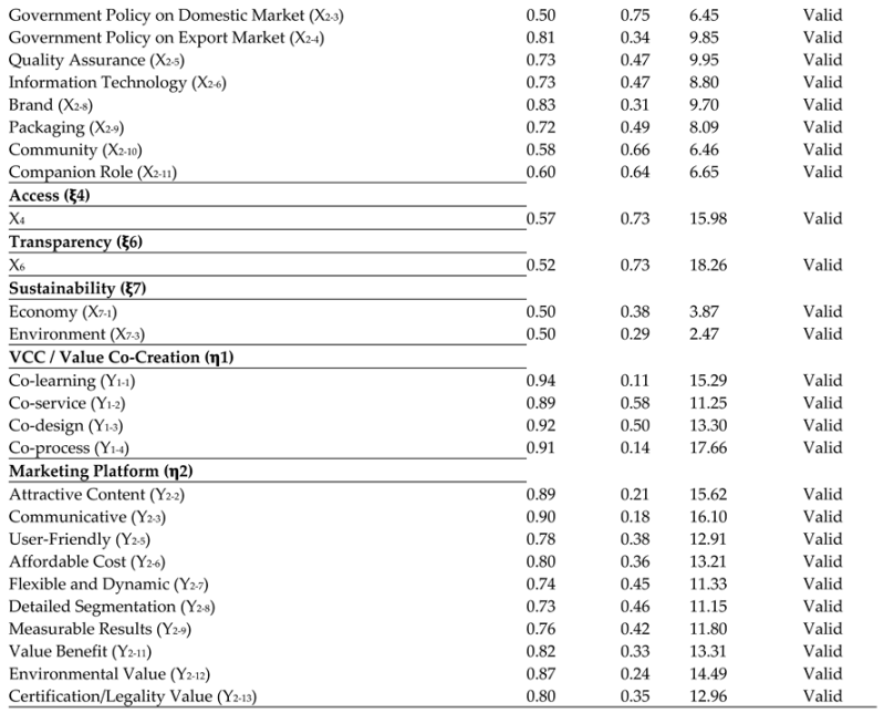
After all the initial assumption tests have been completed, the next step is to perform the SEM model estimation. The initial estimation results using LISREL software version 8.80 produced the Standardized Loading Factor (SLF) values for each exogenous and endogenous indicator/variable, as presented in the following Table 24:
Table 24.
the Standardized Loading Factor (SLF) Values for Each Exogenous and Endogenous Indicator/Variable.
Table 24.
the Standardized Loading Factor (SLF) Values for Each Exogenous and Endogenous Indicator/Variable.
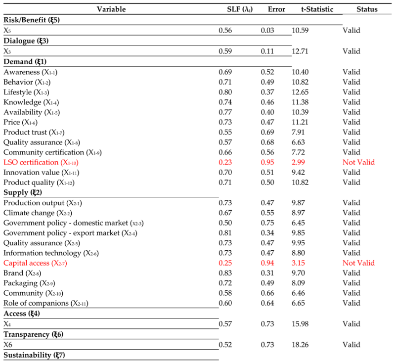
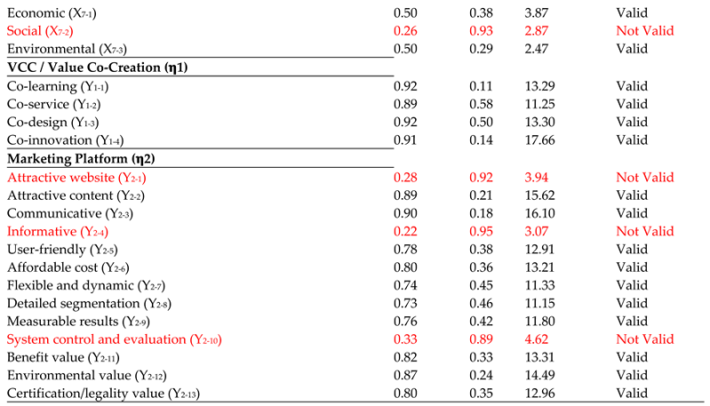
Based on the table above, there are manifest variables that still have SLF values less than 0.50 and insignificant t-values. These include the manifest variables: LSO Certification (X1-10), Capital Access (X2-7), Social (X7-2), Attractive Website (Y2-1), Informative (Y2-4), and System Control and Evaluation (Y2-10). These six manifest variables were subsequently removed, and a re-estimation was conducted. The results of the re-estimation after removing these variables are presented below (the original LISREL output can be found in Appendix 4).
Table 25.
the Standardized Loading Factor (SLF) Values for Each Exogenous and Endogenous Indicator/Variable.
Table 25.
the Standardized Loading Factor (SLF) Values for Each Exogenous and Endogenous Indicator/Variable.
Based on the table above, all manifest variables have SLF values ≥ 0.50, error variance values ≥ 0, and significant t-values. Therefore, the next test can be carried out, namely the reliability test of the measurement model.
Reliability Analysis of the Measurement Model – Confirmatory Factor Analysis (CFA) and Structural Model
This analysis is conducted by calculating the values of Construct Reliability (CR) and Average Variance Extracted (AVE) from the Standardized Loading Factors (SLF or λᵢ) and the measurement errors (eᵢ) using the following formulas: Measurement errors (eᵢ) using the following formulas:
The results of the reliability analysis of the model are presented in the following table.
Table 26.
The Reliability Analysis of The Model.
| Causal Relationship | SLF () | Error | AVE | CR |
| ξ5 ← X5 | 0.56 | 0.03 | 0.91 | 0.91 |
| ξ3 ← X3 | 0.59 | 0.11 | 0.76 | 0.76 |
| ξ1 ← X1-1 | 0.69 | 0.52 | 0.50 | 0.91 |
| ξ1 ← X1-2 | 0.71 | 0.49 | ||
| ξ1 ← X1-3 | 0.80 | 0.37 | ||
| ξ1 ← X1-4 | 0.74 | 0.46 | ||
| ξ1 ← X1-5 | 0.77 | 0.40 | ||
| ξ1 ← Y1-6 | 0.73 | 0.47 | ||
| ξ1 ← X1-7 | 0.55 | 0.69 | ||
| ξ1 ← X1-8 | 0.57 | 0.68 | ||
| ξ1 ← X1-9 | 0.66 | 0.56 | ||
| ξ1 ← X1-11 | 0.70 | 0.51 | ||
| ξ1 ← X1-12 | 0.71 | 0.50 | ||
| ξ2 ← X2-1 | 0.73 | 0.47 | 0.50 | 0.90 |
| ξ2 ← X2-2 | 0.67 | 0.55 | ||
| ξ2 ← X2-3 | 0.50 | 0.75 | ||
| ξ2 ← X2-4 | 0.81 | 0.34 | ||
| ξ2 ← X2-5 | 0.73 | 0.47 | ||
| ξ2 ← Y2-6 | 0.73 | 0.47 | ||
| ξ2 ← X2-8 | 0.83 | 0.31 | ||
| ξ2 ← X2-9 | 0.72 | 0.49 | ||
| ξ2← X2-10 | 0.58 | 0.66 | ||
| ξ2 ← X2-11 | 0.60 | 0.64 | ||
| ξ4 ← X4 | 0.57 | 0.73 | 0.76 | 0.76 |
| ξ6 ← X6 | 0.52 | 0.73 | 0.90 | 0.90 |
| ξ7 ← X71 | 0.50 | 0.38 | 0.56 | 0.72 |
| ξ7 ← X73 | 0.50 | 0.29 | ||
| η1 ← Y2=3 | 0.94 | 0.11 | 0.84 | 0.95 |
| η1 ← Y2-3 | 0.89 | 0.58 | ||
| η1 ← Y2-3 | 0.92 | 0.50 | ||
| η1 ← Y2-4 | 0.91 | 0.14 | ||
| η2 ← Y2-2 | 0.89 | 0.21 | 0.66 | 0.95 |
| η2 ← Y2-3 | 0.90 | 0.18 | ||
| η2 ← Y2-5 | 0.78 | 0.38 | ||
| η2 ← Y2-6 | 0.80 | 0.36 | ||
| η2 ← Y2-7 | 0.74 | 0.45 | ||
| η2 ← Y2-8 | 0.73 | 0.46 | ||
| η2 ← Y2-9 | 0.76 | 0.42 | ||
| η2 ← Y2-11 | 0.82 | 0.33 | ||
| η2 ← Y2-12 | 0.87 | 0.24 | ||
| η2 ← Y2-13 | 0.80 | 0.35 |
According to Yamin (2014), the criteria for good reliability are having an Average Variance Extracted (AVE) value ≥ 0.50 and a Construct Reliability (CR) value ≥ 0.70. Based on the table above, it is evident that the Construct Reliability and Average Variance Extracted values of the latent variables Risk/Benefit (ξ5), Dialogue (ξ3), Demand (ξ1), Supply (ξ2), Access (ξ4), Transparency (ξ6), Sustainability (ξ7), VCC / Value Co-Creation (η1), and Marketing Platform (η2) have met these criteria.
This indicates that the reliability of the measurement model is good and that all latent variables in this model are supported by the data. The next step is to estimate the model and conduct the subsequent test, which is the Goodness of Fit test.
Table 27.
Results of Measurement Model Goodness of Fit Test.
| Goodness of Fit Measure | Fit Criteria | Estimate | Description |
| Chi-Square Statistic | Smaller value | 466.113 | Marginal Fit |
| P-value | P > 0.05 | 0.000 | Marginal Fit |
| Non-Centrality Parameter (NCP) | Smaller value | 239.113 | Good Fit |
| RMSEA (Root Mean Square Error of Approximation) | 0.05 ≤ RMSEA ≤ 0.08 is good fit; RMSEA < 0.05 is close fit; RMSEA > 0.08 is marginal fit | 0.0728 | Good Fit |
| Expected Cross-Validation Index (ECVI) | Closer ECVI value to the saturated model than the independence model indicates good fit | 2.835 | Good Fit |
| ECVI for Saturated Model | 2.774 | ||
| ECVI for Independence Model | 7.662 | ||
| Independence AIC | AIC value closer to the saturated AIC than the independence AIC indicates good fit | 1524.807 | Good Fit |
| Model AIC | 564.113 | ||
| Saturated AIC | 552.000 | ||
| Independence CAIC | CAIC value closer to the saturated CAIC than the independence CAIC indicates good fit | 1623.669 | Good Fit |
| Model CAIC | 774.731 | ||
| Saturated CAIC | 1738.336 | ||
| Normed Fit Index (NFI) | Range 0–1; higher is better. NFI ≥ 0.90 = good fit; 0.80 ≤ NFI < 0.90 = marginal fit | 0.803 | Marginal Fit |
| Non-Normed Fit Index (NNFI) | Range 0–1; higher is better. NNFI ≥ 0.90 = good fit; 0.80 ≤ NNFI < 0.90 = marginal fit | 0.907 | Good Fit |
| Comparative Fit Index (CFI) | Range 0–1; higher is better. CFI ≥ 0.90 = good fit; 0.80 ≤ CFI < 0.90 = marginal fit | 0.927 | Good Fit |
| Incremental Fit Index (IFI) | Range 0–1; higher is better. IFI ≥ 0.90 = good fit; 0.80 ≤ IFI < 0.90 = marginal fit | 0.930 | Good Fit |
| Relative Fit Index (RFI) | Range 0–1; higher is better. RFI ≥ 0.90 = good fit; 0.80 ≤ RFI < 0.90 = marginal fit | 0.769 | Marginal Fit |
| Standardized RMR | ≤ 0.05 = good fit; 0.05 < RMR ≤ 0.09 = close fit; RMR > 0.09 = marginal fit | 0.0804 | Close Fit |
| Goodness of Fit Index (GFI) | Range 0–1; higher is better. GFI ≥ 0.90 = good fit; 0.80 ≤ GFI < 0.90 = marginal fit | 0.931 | Good Fit |
| Adjusted Goodness of Fit Index (AGFI) | Range 0–1; AGFI ≥ 0.90 = good fit; 0.80 ≤ AGFI < 0.90 = close fit; AGFI < 0.80 = marginal fit | 0.894 | Marginal Fit |
Based on the table above, the analysis results indicate that almost all absolute Goodness of Fit (GoF) measures such as RMSEA, NCP, ECVI, AIC, CAIC, NNFI, CFI, IFI, and GFI show good fit values. Only one absolute GoF measure, namely the Chi-Square statistic and its p-value, indicates a marginal fit. Furthermore, the incremental GoF measures also show good fit values, such as NNFI, CFI, and IFI. Thus, it can be concluded that the overall fit of the measurement model is quite good (Good Fit).
Interpretation of SEM Model Analysis Results
After fulfilling all assumption tests, the output of the LISREL Structural Equation Model (SEM) analysis is presented as follows:
Figure 6.
Significance Level of Path Coefficients from SEM Model Estimation Results (Lisrel).
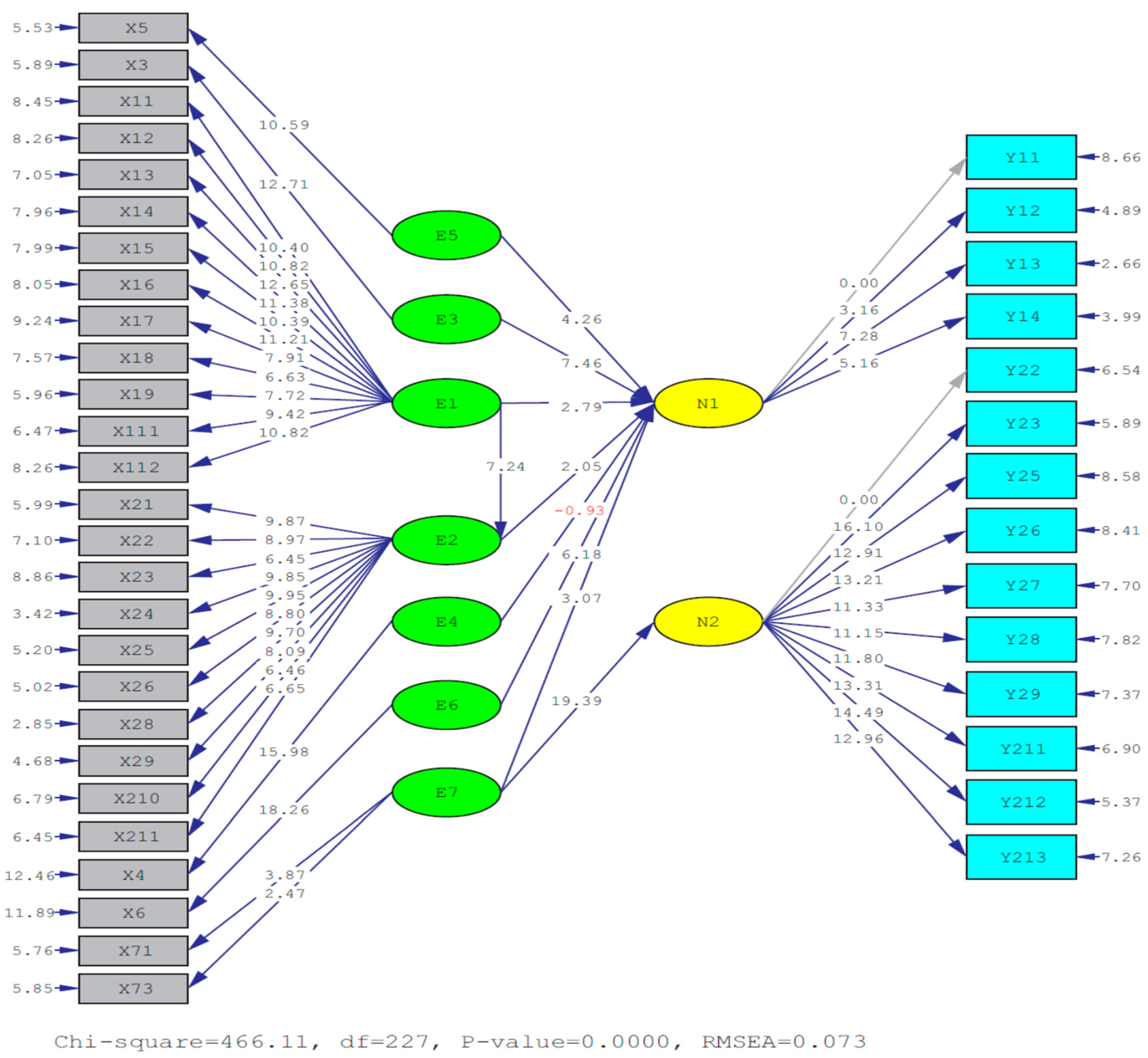
The SEM model can be translated into the following structural equations (the complete results can be found in Appendix 6):
The path coefficient values from the structural equations above, along with their significance levels, are presented in the following table:
Table 28.
Path Coefficients and Significance Levels of Variables.
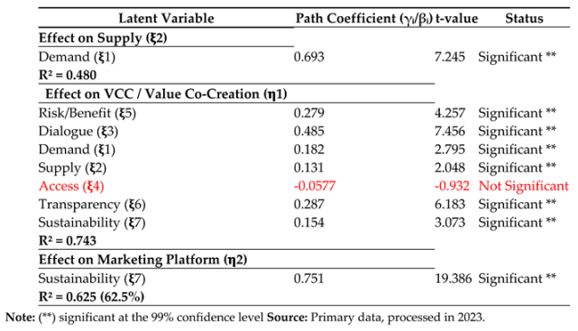
Based on the Structural Equation and the Table above, several conclusions can be drawn: At the 99% confidence level, Demand (ξ1) has a significant effect on Supply (ξ2). Furthermore, at the same confidence level, Risk/Benefit (ξ5), Dialogue (ξ3), Demand (ξ1), Supply (ξ2), Transparency (ξ6), and Sustainability (ξ7) have significant effects on VCC / Value Co-Creation (η1), while the variable Access (ξ4) has no effect on VCC / Value Co-Creation (η1). Additionally, at the 99% confidence level, Sustainability (ξ7) has a significant effect on the Marketing Platform (η2). The following sections elaborate further.
5. Discusion
Discussion of the Effect of Demand (ξ1) on Supply (ξ2)
Based on the Table, the latent variable Demand (ξ1) simultaneously explains the variation in the latent variable Supply (ξ2) with a coefficient of determination (R²) of 0.480 or 48%.The latent variable Demand (ξ1), consisting of the manifest variables: Awareness (X1-1), Behavior (X1-2), Lifestyle (X1-3), Knowledge (X1-4), Availability (X1-5), Price (X1-6), Trust in product (X1-7), Quality assurance (X1-8), Community certification (X1-9), Innovation value (X1-11), and Product quality (X1-12), has a positive and significant effect (99% confidence level) on the latent variable Supply (ξ2), which consists of: Production yield (X2-1), Climate change (X2-2), Domestic market government policy (X2-3), Export market government policy (X2-4), Quality assurance (X2-5), Information technology (X2-6), Brand (X2-8), Packaging (X2-9), Community (X2-10), and Extension support (X2-11). This indicates that improvements in demand indicators for organic vegetables will encourage an increase in their supply. Conversely, if demand indicators decline, the supply will also decrease.
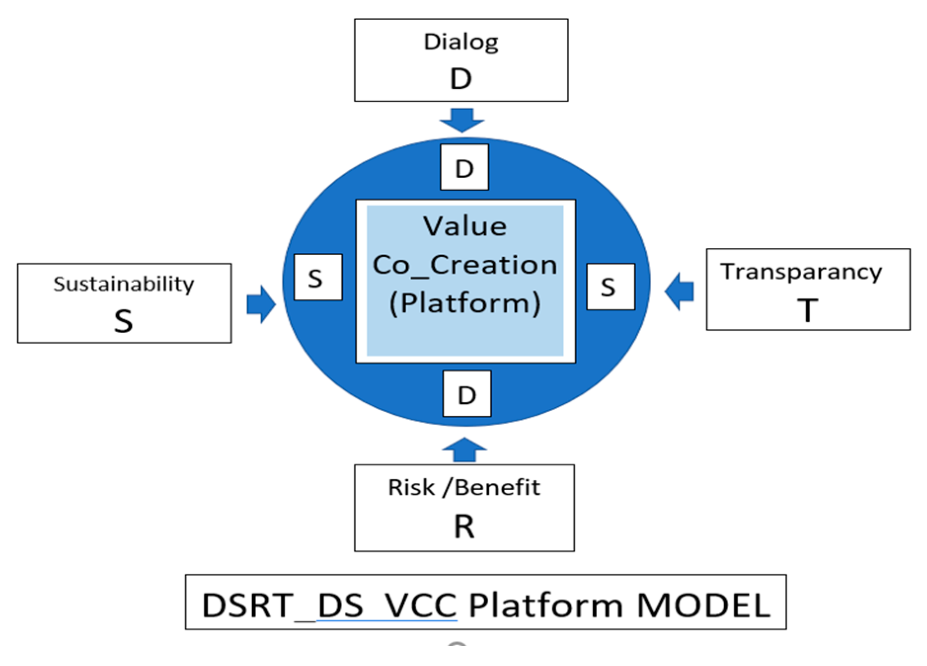
Figure 7.
New DSRT VCC Model.
Germany’s organic wholesale market is projected to increase by 13.8% from 2024 to 2030, due to producers' understanding of consumer demand factors such as product quality, pricing, and product safety assurance (Ministry of Trade, RI, 2013). The supply of organic products in the Mekar Tani Jaya farmer group has increased following the acquisition of SNI: 6729:2016 certification across 94% of its organic production processes. As previously understood, consumers who prioritize product quality standards are more satisfied with the implementation of SNI organic certification (Maryowani, 2012). The largest organic vegetable producer in Cibodas, Bandung Regency, ‘Saung Organik’, has adopted post-harvest handling strategies such as eco-friendly packaging, product labeling for safety, and INOFICE certification for packaging houses, contributing to high demand from distributors and modern markets to become loyal customers.
Research Contribution to the Organic Agriculture Business. The results of this study make a significant contribution to the practice of sustainable organic agriculture. Challenges remain in implementing environmentally friendly and sustainable agricultural practices, particularly across various agribusiness subsystems: in the upstream input supply, on-farm production or cultivation processes, downstream in marketing and distribution, as well as in the supporting subsystems related to partnership institutions.
The Value Co-Creation (VCC) Business-to-Customer (B2C) model for organic vegetables offers new insights into both theory and practice of sustainable organic farming by examining the dynamics of demand and supply for organic vegetables. The Collaborative Business Model serves as a standard for conducting business in the organic vegetable sector specifically, and organic farming practices more broadly. The creation of shared value between producers and consumers (value co-creation) in the B2C context—through innovations such as co-learning, co-service, co-design, and co-process—can guide business practitioners and organic vegetable farmer groups in applying these elements as part of their marketing strategies.
Marketing of organic vegetables can experience increased supply as a result of higher demand driven by a broader customer segment across various age groups, income levels, behaviors, and lifestyles. The marketing platform, which is built upon VCC principles for organic vegetable commodities, has proven effective and beneficial for consumers from Baby Boomers to Gen X, Y, Millennials, and Gen Z. The development of co-learning, co-service, co-design, and co-process features on the marketing platform can further boost demand, which in turn increases supply.
One of the key contributions of this research lies in its emphasis on the importance of increasing demand for organic vegetables not merely through production processes, which tend to focus solely on profitability. In reality, field data show that consumption of organic vegetables remains low due to higher prices compared to conventional vegetables. In fact, the cost of organic vegetable production is often lower than that of conventional farming. The price of organic vegetables is aligned with their production value—higher prices reflect higher quality. However, lower-income consumers still face challenges in accessing healthy vegetables.
6. Congclusion
The following are the conclusions from the research conducted: The demand and supply of organic vegetables in West Java need to consider prices that align with market equilibrium and ensure that the quantity of each type is appropriately prepared by each organic vegetable business. The sustainable B2C VCC (Value Co-Creation) model for organic vegetables is the DSRT model, which enhances the existing DART model. Therefore, a shift in mindset is needed: the value of organic vegetables should be based on necessity rather than price. When all stakeholders—farmer groups, entrepreneurs, and consumers—understand the intrinsic value of organic vegetables as a basic need, rather than a luxury item, demand will naturally increase, followed by a rise in supply.
Author Contributions
Conceptualization, K.R.N, D.Y, W.K.A and T.L; Data curation K.R.N; Formal analysis K.R.N and D.Y; Funding acquisition D.Y; Investigation K.R.N and W.K.A; Metodology K.R.N. D.Yand T.L; Project administration : D.Y; Resourches W.K.A and T.L; Software K.R.N; Suvervisor; T.L; Validation K.R.N, D.Y, and T.L; Vicualization K.R.N; Writing- original draft ; K.R.N; Writing-review and editing K.R.N, D.Y, W.K.A and T.L; All aouthors have read and agreed to the published version of the manuscript. version of the manuscript.
Institutional Review Board Statement
Not applicable.
Informed Consent Statement
Not applicable
Data Availability Statement
data will be made available upon request
Conflicts of Interest
The authors declare no conflict of interest.
References
- Adesemowo, Abayomi Alli A, Arogundacle. 2020. Aplikasi Seluler Marketspace Cerdas Untuk Memasarkan Product Organic. Proceeding.
- Alse Fagestrom and Geogrghita Ghinea. 2020. Co Creation of Value Trough Social Network Marketing, A Field Experience Using Facebook Campaign to Increase Conection Rate. Human Interval Journal, Part II.HC II.2011 Sringer-US lag Berlin Heideberg.2020. [CrossRef]
- Arif Zulkifli. 2020. Green Marketing Redefinition Of Green product, Green Price, Green Place, Green Promotion. Graha Ilmu Jakarta.
- B Evanddisson, G Nog CZ, MiinR Fithi. 2011. Does Service Dominat Design Resnet In a Boller Service Sistem? Journal Service Management. [CrossRef]
- Becoause, R,Harjiyatni, F. R. , Princess, W. H. , Kresnanto, N. C. 2021. Green behavior in organic products: Policies approach. Journal. [CrossRef]
- Boz Ismet. 2019. Possibilities of Improving Organic Farming In Turkey. International Journal.Proceedings. [CrossRef]
- Budi Kusumo RA, Charina A. 2021. Communication Network Analysis on Organic Vegetable agribusiness in West Bandung Regency. Journal of Counseling Vol.17 no.2.
- Buyun Liu, Cyntia L, etAll. 2022. Perspective Organic Food Consumption During Pregancy and Thev Potential Effect on Maternal and Of Bring Healt. Owral Pre Prof Journal. [CrossRef]
- Christine HvitsandaRuth Kjærsti Raanaasb SigridGjøtterudc Anna Marie Nicolaysena. 2022. Establishing an Agri-food living lab for sustainability transitions: Methodological insight from a case of strengthening the niche of organic vegetables in the Vestfold region in Norway. Journal Agricultural System. [CrossRef]
- DahlStrom, P.2020. Green Marketing opportunity for Innovation, New York, Book Surge.
- Deliana Y. 2018. Business Model for Promoting Organic Vegetables. IOP Converece Series Erath and Enviromental Sciece. [CrossRef]
- __________ 2012. Market Segmentation of Organic Product at Bandung West Java Indonesia International Journal.
- _. 2012. Customer preference On Organic and An Organic Vegetables in Bandung West Java Indonesia. International Journals.
- . 2012. Hierachy of Customer Decision in Buying Organic Vegetable in Bandung West Java Indonesia. International Journals.
- . 2016. A Picture Is Worth a Thousand Words Understanding Consumer Interaction in Organic Packaging. International Journals.
- . 2016. Marketing & Value Chain of Gedong Gincu Mango with Its Labeling and Packaging. [CrossRef]
- . 2019. Generation Green Marketing. Scientific Oration at the Inauguration of Professors Unpad.
- _. 2019 The Role of Green Marketing for Sustainable Agriculture. Books of Kotler, Philip and Amrstrong Gary. 2008 Principles of Marketing. InEdition Volume 12. Jakarta Erlangga.
- . 2008. Principles of Marketing. Volume II 12th Edition. Jakarta Erlangga . 2009. Marketing Management. Volume I 13th Edition. Jakarta Erlangga.
- ____________. 2009. Marketing Management. Volume II 13th Edition. Jakarta Erlangga.
- Fakhrul Islam M and Karim Z. 2021. Sustainable Agricultural Management Practices and Ebterprise Development for Coping with Global Climate Change. ChapterBook.
- Fan Jun. 2019. Influence of Virtual CSR Gamification Design Element On Customers Antiniance Intention Of Participing In Social Value Co Creation The Mediation Effect Psycological. www. New emerald/Insight. 13555855. [CrossRef]
- Granroos C and Heinonen K. 2015.Value Co Creation : Critical Reflections. Hanken Scholl Economic. Book.
- Hakseung Sin, Richard R Perolue, Mario Pandelowrence. 2020. Managing Customer Review For Value Co Creation A Emporment Theori Perspective. Travel Research of Journal. [CrossRef]
- Hasibuan I. 2020. Organic Farming – Principle and Practical. Tidar Media Jakarta. Book.
- Hubies M, Najib M, Widyastuti, Wijaya NH. 2013. Farmer-Based High Value-Added Organic Food Production Strategy. JIPI -Indonesian Journal of Agricultural Sciences. December.
- Hunger, J. David & Thomas L. Wheelen, 2003 Manajemen Strategi edisi II. Yogyakarta.
- J Chong G Chen, D Zheng. 2020. Design Entroppy Theory a New Design Methodologys Smart PSS Development. Journal. [CrossRef]
- Katrien Vorleya. 2015. The Co Creation Experience From The Customer Perspective Its Measurenment And Theterminants. www.emerald insight.com/1757-58118 htm. [CrossRef]
- Kattel RR, Nainabasti A.2020. Consumers Attributes and Preference Organic on Organic Agriculture Product in Nepal. Proceedings of the AgriculturaleMarketing Conference.
- Kementrian Perdagangan RI. 2013.n Market Brief Pasar Produk Organik di Jerman. ITPC Hamburg.
- Khairawati S. 2021. Marketing Mix Strategy in Marketing 5.0 Articles.
- Kartajaya Hermawan. (2009). New Wave Marketing, The World is Still Round the Market is Already Flat. English: Gramedia.
- Kondraslka, IC daTytarenko L, Kalnik O, Novytska I. 2018. The Blockchain Technology as a New Approach of Promoting Organic Product to The Market. International Journal of Enginering and TechnologyVol.August 7 (790-795).
- Kotler, P, Kertajaya H, Setiawan i. 2021. Marketing 5.0 Technology for Humanity. E- Book, Wiley New York.
- Kritiadi A, Hartoyo. Yusuf E, Sukandar D. 2021. Online Modeling of Community Relations Management in the formation of value co creation in the BroadBand Cellular Telecommunications Industry of Indonesia. Journal.
- Laura TM, Vand Grint, Anthony M , Evans Olgastarova. 2021. Good Eats, Bad Intentions? Repotational Cost Of Organic Consumption . Environmental Psychology Journal. [CrossRef]
- Maulana E, A 2021. Qualitative Methodology in Marketing. Pustaka Etnomark Jakarta. Book.
- Mayrowani. 2012. Developing Organic Agriculture in Indonesia. Journal.
- Miles, M.B & Huberman A.M. 1984, Qualitative Data Analysis. Translation by Tjetjep Rohendi Rohidi. 1992. Jakarta: University of Indonesia Publishers.
- Millis, John W, S Walker, Orville CJR. 2010. Marketing Management a Strategic Decision Making-Approuch (7th edition). Singapore. MC eawhill.
- MónicaDuque-AcevedoabLuisJ.Belmonte-UreñabEduardoTerán YépezcFranciscoCamacho-Ferrea. 2022. Sustainability and circularity in fruit and vegetable production. Perceptions and practices of reduction and valorization of agricultural waste biomass in south-eastern Spain. Journal Of Enviromental Management. [CrossRef]
- N Brahnosa, K Nojer, H Want Der Hart.2020. Innovatife a public Service Design Developing A Co Creation Tool For Publick Service Innovative. Journal. [CrossRef]
- Nusraningrum D, Santoso S, Gunawijaya J, Gading DK. 2021. Green Operation Management with Green Business and green Marketing Perspective. Psycology and Education Journal.
- Oesman, Yevis Marty. 2010. Successfully Managing Marketing MIX, CRM, Customer Value,Customer Dependency. Bandung Alfabeta.
- Ottman, J.A. 1998. Green Marketing of Oppourtunity for Innovation. New York-Book Surge.
- Wewthen, P Greffen. 2017. Designing Service Dominant Business Model. Journal.
- Patten J. 2010. Green Intention, creating a green value Stream to Compete and Wind. International Journals. [CrossRef]
- Pe'pin A, Morel K Hayo MG Van der Werf. 2021. Data on Structure and Farming Practicies of France Organic Vegetables Farm. With focuse on The Use of Input and the Socio-Economic Context. International Journals. [CrossRef]
- Prime, T. 2014. Financing System for Applications in High-Value Horticultural Supply Chain Management. National Journals.
- . 2016. Durian Suply Chain Characteristic Indonesia. National Journals.
- . 2016. Lingking Mango Farmer to Dynamic Market Through Transpparant Margin Parnership Model. International Journals. [CrossRef]
- Pistol L. 2020. The & 7Ps and 1G that Rule in The Digital World the Marketing Mix. Chapterbook.
- Prahalad, C.K. Prahalad, C.K. (2004):"The co-creation of value,". Emerald Journals database: vol. 68, p.23.
- Purnomowati, NH Asrihaspari, A. 2021. Green Community Empowerment Business Model to Recognize Solo Green City: A Case Study. Scientific Journal of Management.
- Rajadurai J Zahari A, at all. 2021. Investigating Green Marketing Orientation Practices Green Small and Medium Enterprise. International Journal. [CrossRef]
- Rahmawanti, A.F.D. 2011. Pengaruh Gamification Pada Program Loyalitas Terhadap Pengguna Marketplace Dengan Menggunakan Expectation Confirmation Model ECM. Skripsi.
- Rahmawati M, Ruslan A, Bandarsyah D. 2021. The Era of Society 5.0 as The Uniffication of Humans and Technology A Litertur reviw on Materialism and Existentialism. Journal. IOP Conference Series. [CrossRef]
- Ramjan. K.R. 2020. Bringing The Individual In to The Co Creation Of Value. Service Marketing . Vol 33. No.7. [CrossRef]
- Razo, Zapala, EK Chew, D Sangragi. 2018. VIVA, Visual Language to Design Value Co Creation. Journal. [CrossRef]
- Rizqianingsih, DU, Widodo, A. 2021. The Effect of Green Marketig and Service Quality on Customer Loyalty with Customet Satisfaction as an Intervening Variable (Case Study at Strutbuck Coffee Surabaya). Journal.
- Renata Lúcia Magalhães deOliveiraaIgor VieiraSantosaGuilherme FonsecaGracianobAndré AugustoCunha LibâniobLeiseKelli de OliveirabLílian dos Santos Fontes PereiraBracarensec. 2021. A sustainable approach for urban farming based on city logistics concepts for local production and consumption of vegetables. Journal research In Transportation Economics. [CrossRef]
- Sagita Chan SRO. 2021. Horticultural Plant Seeding and Breeding Industry in Indonesia: Current Conditions and Business Opportunities. Hortuscholer's journal. Vol 2 No.1Setyowati L, Nasir Ahmad D. 2021. Utilization of Big Data in the Era of technology 5.0. Journal of Community Service Vol.1 No,2.
- Setiawan,I, Supyandi.D, Rasiska S, Judawinata G. 2018. Pertanian PostModern ; Jalan Tengah Vertikal Generasi Era Bonus Demografi Membangkitkan Peradaban Nusantara. Penebar Swadaya. Jakarta.
- Seungwoa Hen, Yokyung Lee. 2022. Analisis Of The Impact and Lyfe Stile Consumption Organic Food In South Korea. Helion Jornal. [CrossRef]
- Sugiono. 2012. Quantitative, Qualitative, and R and D Research Methods. Bandung Alfabeta.
- Sukmawani, R. 2018. Methods of Determining Superior Commodities. UMMI Perss.
- Sukojo Herdin, Sumanto Radi X A. 2012. 7P Marketing Mix Analysis (Product, Price, Place, Participant, Process, Phisical Evident). Nasional Journal.
- Voronka Q Yu and Kovaleva IV. 2020. The Sustainable Socio-economic Development Of Rural Areas inTerm of Development of Organic Farming. Jurnal Sucita S, Novan Prasetya M. 2021.Indonesia Singapore Cooperation in Export of Imports of Agricultural Commodities 2018. Fisk Journal April Vol.2 No.1.
- Yud Buana, Iasnawirakma, dkk. 2019. Konseptualisasi Value Co Reation Dalam Konteks Customer To Customer ( C2C). Jurnal Pengabdian dan Kewirausahaan. Vol 3. No.1. [CrossRef]
- Wai Kuan Alice,Cheac Asaro Aigbogun. 2022. Exploring Attitude Behaviour Incontsitent In Organic Consumption Daring Covid 19 Pandemic In The Kiang Valley Malaysia. Cleaner and Responsible Consumption Journal. [CrossRef]
- Weiping Yu, Mingli He, Xiaoyun Han and Jun Zhou. 2021. Value Acquistion Value Co Creation The Impact Of Preceived Organic Grocerant Value On Customer Engagement Behaviour Through Brand Trust . Frontresrin Psychology Journal. October. [CrossRef]
- Juga 40 referensi terkait VCC platform product sayuran organic.
Disclaimer/Publisher’s Note: The statements, opinions and data contained in all publications are solely those of the individual author(s) and contributor(s) and not of MDPI and/or the editor(s). MDPI and/or the editor(s) disclaim responsibility for any injury to people or property resulting from any ideas, methods, instructions or products referred to in the content. |
© 2025 by the authors. Licensee MDPI, Basel, Switzerland. This article is an open access article distributed under the terms and conditions of the Creative Commons Attribution (CC BY) license (http://creativecommons.org/licenses/by/4.0/).
Copyright: This open access article is published under a Creative Commons CC BY 4.0 license, which permit the free download, distribution, and reuse, provided that the author and preprint are cited in any reuse.


