Submitted:
14 April 2025
Posted:
15 April 2025
You are already at the latest version
Abstract
From the regular collision time, τcee, due to multiple Coulomb collisions between electrons an effective electron radius is proposed using the kinetic theory in plasma physics and considering we deal with what we will call a Lorentz-like gas. The effective or equivalent electron radius is deduced by corresponding the total cross section with a collision radius that can be related with the length of the electron and depends on the temperature and density a=a(n;T). This is quite unusual, but ultimately it is a measure that describes an effective radius of the electron based on supposing collision of rigid spheres corresponding to the electrons in a Lorentz-like gas with temperature and density. Unlike other electron size proposals where fixed parameters are taken, the electron radius is deduced from a many-particle system. τcee is compared with the electron-electron relaxation time, τee, obtained calculating the cross section for the momentum transfer. Taking into account typical fusion conditions (TOKAMAK), the equivalent electron radius aT as well as the corresponding electron-electron collision and relaxation times are calculated. Assuming that electron describes a diffusion equation based on Stokes law of viscosity, the friction coefficient α is calculated using the relaxation time and the dynamic viscosity η is deduced from the first order approximation of the Chapmann-Enskog theory for hard-sphere electrons.
Keywords:
electron radius
; multiple collisions
; Plasma
; TOKAMAK
1. Introduction
Among the problems of modern theoretical physics is the complex question of the size of the electron radius. However, accepting the existence of a finite electron radius is not compatible with the premises of the theory of relativity. Indeed, the electron is a charged particle considered as point-like because this model is consistent with Quantum Electrodynamics (QED). On the other hand, a point-like electron (zero radius) generates serious mathematical difficulties because the electron’s own energy tends to infinity [1,2,3]. Although from the energy uncertainty relation an upper limit of the electron radius of [4] can be derived, a more sophisticated study by means of the observation of a single electron in a Penning trap suggests that the lower limit of the particle radius is [5]. However, certain theories have proposed distinct electron sizes to describe some effects in different phenomena; namely, among others:
Let us analyze each proposal by describing in greater detail the case of what we call a Lorentz-like gas and its effective radius. The latter yields the existence of an effective electron radius due to collective effects, which is the objective of this work.
1.1. Classical Electron Radius
The classical electron radius [2] is a combination of fundamental physical quantities that defines a length scale for problems that involve the interaction of an electron of charge e with electromagnetic radiation. It consists of relating the energy of the relativistic mass of the electron with the classical energy of electrostatic self-interaction of a homogeneous charge distribution. The classical electron radius is motivated by the following reason: if one considers that the electron’s energy at rest can be likened to its mass , we have
hence
It should be noted that the Thomson scattering length, the Lorentz radius, and the classical electron radius represent the same thing. Note that it is related to the characteristic time expressed in , appearing in the Lorentz-Dirac equation [1] or the Abraham-Lorentz equation [10,11,12]. Indeed, if a particle travels at the speed of light for a time it travels a distance practically equal to the size of the classical radius of the electron, ; let us see:
But this model leads to a difference in mass by a factor of when a correct relativistic model is implemented [13]. This shows that the classical electron radius concept carries certain contradictions when used universally.
1.2. Reduced Compton Radius
The Compton radius of the electron, which is obtained from photon scattering experiments, is given by (in CGS units) [6]
where is the fine structure constant. Note that in this scheme the interaction is with photons and that the Thomson scattering radius is compatible with the reduced Compton radius .
The reduced Compton radius of the electron by means of the Zitterbewegung [6] is obtained by considering that the momentum and position of the electron are determined by a probabilistic interpretation of the wave function described as a cloud of electron density. These semiclassical models have common features that allow us to better describe the nature of the electron; for example, they all consider that the Zitterbewegung, a "trembling motion" of the electron at the speed of light, is a real oscillatory motion of the electron, and they arrive at certain results proposing at a given moment that this last effect combined with the Compton effect could give us the so-called reduced Compton radius as in Eq. (5).
1.3. Nuclear Electron Radius
1.4. Electron Radius from Einstein’s Dual Theory
The Einstein dual theory [9] (Proper Time) of relativistic quantum mechanics with a single approach when minimal coupling is turned off, three distinct dual relativistic wave equations produced reduce to the Schrödinger equation. This model shows that a new formula for the anomalous magnetic moment of a charged particle is obtained from the dual Dirac equation. As long as the electron radius is considered to be , we can obtain the exact value of the electron g-factor; that is,
1.5. Lorentz-like Gas and Collision Times
The Lorentz gas is an ideal gas first proposed by Dutch physicist Hendrik Antoon Lorentz in 1905 [14] to model the thermal and electrical condition of metals. He assumed that the electrons in the conduction band behave as an ideal gas with no interaction between them until they collide with the nuclei of atoms, which are practically on the time scales in which electrons remain in a certain area. Thus, the Lorentz model consists of a set of fixed obstacles (typically hard-spheres), which represent on one hand point electrons and on the other atomic nuclei at the vertices of a lattice. The electrons have free movement as long as they do not collide with the a nucleus. When the collision occurs, the particle is deflected following a mirror reflection. To make this model, Lorentz made a Boltzmann-type approximation, with which he implicitly assumed that the density of atomic nuclei was low. Physically, this makes sense if one reinterprets atomic nuclei as defects in a lattice, rather than as ions.
In subsequent years and especially in recent decades, modifications to this model have been studied, where the type of lattice, the shape of the obstacles, the number of dimensions, the reflection rules, the presence of fields, whether electric or magnetic, etc., are varied. Furthermore, this model has been relevant both in the fields of physics and mathematics. In physics, the model is important for studying transport problems, statistical physics, dispersion problems, molecular dynamics simulations, and even as a model to study a photonic crystal [15]. On the other hand, in mathematics, the model has illuminated the field of probability and dynamical systems.
1.5.1. Lorentz-like Gas
It should be noted that a classical gas of electrons cannot be compared with one of the species of a plasma at high temperatures as one might think. This is because in the Lorentz gas the electron-electron collisions are neglected, unlike in the kinetic theory of gases. In fact, it is worth highlighting at this point [17,18,19], that for each species the internal energy is defined by defined by
where and represent the density of particles, the energy per unit particle, the mass, the velocity of the species and the distribution function of the species, respectively. The kinetic energy of the particles is assumed to be much higher than the average potential energy of the interactions. Plasma thermodynamically resembles an ideal system; that is, an ideal gas where the interaction is described as collisions between the particles is called a Lorentz gas.
In the case of ions and electrons we have a two-fluid description of the plasma used in many texts [20]. When the collision time between the electrons and the ions is much larger than the collision time between the electrons and the electrons, we can deal with a one-fluid model composed of electrons without accounting for the ions, and we can affirm that we are dealing with a Lorentz-like gas of electrons.
The correlation function between electrons gives an equation of state where the Debye length is considered [20,21,22]. This is the Balescu-Lenard equation which has the form of the Fokker-Planck equation , but it takes into account the shielding and dielectric properties of the plasma. In fact, the so-called reduced distributions, in particular the second reduced distribution gives a two-particle correlation function (electron-electron with charge e)
where
Consequently when the cross section is calculated for multiple Coulomb collisions the Debye length appears. Completing the Fokker-Planck description of a collisional effects in a fully ionized plasma gives naturally the Landau collision operator which includes the Coulomb logarithm. Since the Coulomb logarithm includes the Debye length, the cross section does not diverge. This is justified for inert plasmas of high temperature and/or low density. That is, the weak coupling condition described by the plasma parameter which represents the number of particles in a sphere of Debye radius. [18]
is satisfied. Equivalently, we ask that the coupling plasma parameter, , fulfills
where the occupation length for each charge and represents the mean distance of closest approach,
In the Lorentz-like gas, we can then say that we are analyzing a gas of electrons since we are considering that the ion gas is ignored. Indeed, the scattering section is related to the so-called Coulomb logarithm defined by
where represents the Debye length [18] which takes into account the shielding performed by the electrons on the electrons and which is taken as the mean distance of closest approach or the De Broglie length.
1.5.2. Collision Times
On the other hand, whenever we deal with a plasma, the dispersion effect between the particles is fundamental. In this order of ideas, the cross section is related to the collision time [23]; that is to say:
where represents the total cross section and v is the thermal velocity. Our purpose is to compare the multiple collision time of the electron-electron with the regular binary collision time defined from the classical kinetic theory of gases, Eq. (15), taking the electrons as perfectly rigid spheres. We need to consider the high-energy limit , being a the radius of the perfect rigid sphere particle; that is: for the Quantum case [24]. However, for our classical point of view, we will consider that . We have (see [18] Eq. (4.58))
An analysis shows that in fact for temperatures greater than , the species made up of electrons behaves completely like an ideal gas but the interaction is reduced to shocks described by a cross section that is equivalent to rigid spheres with a radius a.
In the two-fluid model, the collision times are not calculated due to binary collisions but to multiple collisions, and we have to differentiate between the collision times due to multiple collisions and , and the relaxation times and between electrons with electrons, between electrons with ions (and vice versa) and between ions with ions, respectively. However, for many authors the collision time due to multiple collision are similar to the relaxation time, they are expressed by just one expression [18,19,25,26,27]:
where and represent the ion and electron masses, respectively. It should be noted that in some texts, instead of talking about relaxation time, they talk about momentum transfer time, which is consistent with their deduction [27,28]. Although the collision times of ions with ions or of ions with electrons are very large compared with the collision time of the electron with electron, the electrons can be treated as a Lorentz-like gas, and the interaction reduces just to collisions between rigid spheres and therefore as an ideal gas. However, we will see that the collision time due to multiple collisions is different from the relaxation time [29,30,31].
Finally, the aim of the work is threefold. The first objective is to show that there are several characteristic times in a Lorentz-like gas, namely: the duration time of a collision, the binary-like collision time, the collision time due to multiple collisions, and the relaxation time. The binary-like collision time is meaningless but has an application when calculating dynamic viscosity. It will be seen that although it is assumed by many authors for an isotropic solid, such as a metal, that the multiple time is equal to the relaxation time [32], we will see that the first is smaller than the second coinciding with what is said in reference [29] for metals contrary to some affirmations [32]. The second purpose is to find the effective or equivalent radius of an electron in a Lorentz-like gas that simulates the same effects as point electrons. The third result consists of finding a technique for obtaining the dynamic viscosity owing to the collisions of electrons with electrons.
The article is organized as follows. In Section 2, the different times are defined and calculated as functions of the temperature and the density. Section 3 is advocated to calculate the effective or equivalent radius of the electron in the Lorentz-like gas as a function of the temperature and the density and for the particular values of the temperature and the density in a TOKAMAK. The dynamic viscosity is deduced from the first order approximation of the Chapmann-Enskog theory for hard-sphere electrons. in Section 4. In Section 5, a discussion of the applicability of the above results is presented.
2. Times in an Electron Plasma (Lorentz-like Gas)
The size of the electron and its relationship to the Debye length are a seemingly unrelated topic. However, the Lorentz-like gas represents one of the physical systems that can contribute to finding such a relation. Indeed, by equating Eqs. (16) and (17), we can obtain the effective electron radius, where the Debye length is used via the value of . However, before that, we must understand certain aspects of some characteristic times associated with electrons in the Lorentz-like gas.
2.1. Characteristic Times
Let us define some important times in plasma physics. We will restrict ourselves to electrons only.
- The duration time of an electron collision is the time in which the interaction between two electrons lasts;
- The collision time or the free path time is the time that passes between each collision ( for the TOKAMAK);
- The relaxation time is the time in which the particles slow down due to Stokes’ law.
2.2. Hierarchy of the Different Times
The following relationship must be fulfilled.
This is because in order to consider the particles as colliding spheres the duration time of the collision must be much smaller than the free path time. In addition, the collision time should be smaller than the relaxation time because it is assumed that there must be many collisions for a particle to change direction by 90° [18,20]. Normally, one should say [30], but already considers multiple shocks in the case of electrons and therefore it is only needed that . In fact, for metals one has [29].
2.3. Duration Time
The duration time of a collision corresponds to the time in which the particles interact. When the collision is Coulombic, obviously this time is infinite, but one can think that the duration of the collision corresponds to the value of the interaction pulse (see Ref. [2] Sect. 11.10, Eqs. (11.153) and (11.154), Sect. 14.5 Eqs. (14.64) and (14.65) and Chap. 15 on Bremsstrahlung, etc). Indeed, the duration time is described as the time in which the fields are appreciable (as if it were a pulse). We call the duration time of the collision of an electron-electron. Therefore, we must consider the duration time of the collision as the duration of the pulse. Finally, in a relativistic way the measure of the interval of time in which the fields are appreciable is:
For the non relativistic case, we have
It is convenient to define a large angle scatter, or a close encounter, as one that results in an angular deflection of the incident particle of 90° or more. The impact parameter resulting in a scattering of 90 is [18,20] which coincides with the mean distance of the closest approach in Eq. (13).
Hence:
This implies that the duration time in a TOKAMAK, , taking
is of the order of
This is a longer time than the characteristic time of the electron, which is on the order of . On the other hand, each electron corresponds to a maximum radius of (occupation length for each charge)
Consequently, the distance L traveled by a typical electron during must be much smaller than ; that is:
This means that the particles barely move during the collision and their path is less than the occupation length for each charge. This will allow collisions to be considered instantaneous compared to and for a TOKAMAK. Note that L will be of the order of magnitude of the effective radius or equivalent that we will calculate later by using in Eq. (16). In fact, the latter proves that one cannot consider only binary collisions as those that describe the deflections of electrons instead of taking into account multiple collisions, since throughout the distance traveled during a binary collision, the Debye length is much larger (), and this explains why during a binary collision the electron feels the interaction with the other charges. Therefore, a good description of the interaction between electrons consists in considering multiple collisions.
2.3.1. Stochastic Force, Stokes’ Model
If we want to occur a Stokes’ force and a stochastic force, we must consider that the duration time must be much shorter than the relaxation time (also called ). We must first understand some properties of this Langevin force (in one dimension for simplicity) [34].
where F represents an stochastic force. We first assume that the average over the ensemble must be zero.
because the equation of motion of the average velocity must be given by
where is the friction coefficient, and the relaxation time is
If we multiply two Langevin forces at different times we assume that the average values are zero for different times which must be greater than the duration time of the collision ; that is:
Such a noise force with the correlation described by Eq. (32) is called white noise. This assumption seems reasonable since collisions of different fluid molecules with small particles are approximately independent. Typically, the duration of a collision, , is much shorter than the relaxation time of the small particle. We can then take as a reasonable approximation, giving
with .
Then it is needed that
hat is,
Considering that the relaxation time and the correlation time are of the same order, we need to determine the following.
For a TOKAMAK, . This is accomplished in a TOKAMAK.
2.4. Collision Time or Free Path Time
A gas is out of equilibrium when it is not described by the Maxwell-Boltzmann distribution function. The most common case is when the temperature, density, average velocity, etc., are not the same throughout the gas. Equilibrium is achieved by the transport of mass, energy, and momentum from one part of the gas to another. The transport mechanism is due to collisions or molecular interactions. The typical distance over which these effects develop is known as the mean free path or distance and represents the average distance a particle travels between each collision. The number of collisions that occur per second per unit volume at a point is [23]:
In fact, we can perform the integral on the solid angle since the integral is free since it depends only on ,
On the other hand, each collision involves two particles (binary collisions), so we can conclude that the total number of free paths per unit of time and volume is . Since the density of particles is n, it follows that the average number of free paths per unit of time and volume of a particle is . The average free path for a particle is the velocity multiplied by the average time between each collision.
and if in one second a particle has free paths then each free path occurs in
Hence
We can always take a good approximation to by comparing collisions between rigid spheres of diameter a, which is a constant, or simply consider as a constant.
Let us now consider that the Maxwell-Boltzmann distribution is very close to our non-equilibrium distribution, then
where
The integration is immediate and we arrive at (),
Then
where is for rigid sphere. Note that the collision time is deduced from the Z-function and not from the collision operator used to obtain the relaxation time [18].
2.4.1. Example
Let us calculate a typical case:
2.4.1.1. H2 at its Critical Point
H2 at its critical point [35] , with the following data
Obtains
which corresponds to Huang’s result[23]. The collision time is equal to
This coincides with Huang’s proposal around [23].
On the other hand, following Stokes, one must have a relationship
Let us now compare with
This cannot be the case, since the system cannot decay before colliding. The reason is that in the derivation of Eq. (49), a continuum cannot be established for particles of the same size as is required to determine the relaxation time. Let us also check the Reynolds number.
where the dynamic viscosity is . That is, R is not small, and therefore, Stokes’ formula for obtaining the relaxation time does not work. Therefore, we should expect that it will not work for calculating the relaxation time for electron-electron collisions either, as we will see. However, an interesting relationship will emerge when Stokes’ theorem is used for the collision between electrons. Indeed if is replaced in Stokes’ formula (Eq. (48)) by a consistent result will be obtained. This will be analyzed in Section 4.
2.5. Rutherford Scattering
Rutherford scattering is historically very important because it was used to determine the structure of the atom. Indeed, it represents the most important scattering because it is related to the fundamental interaction at the atomic level, namely the Coulombic interaction. If we consider the interaction to be repulsive, that is (), the result is [36]
where , l is the angular momentum and . Since cannot be negative, and also . This last point simply limits the motion. In fact, it should be noted that does not define the initial position. In fact, represents the axis of symmetry. Therefore, the following representation is better: let be the angle such that
Therefore, it is clear that the angles and are such that (see Figure 1 and Figure 2). We know that
where s is the impact parameter. As we have , hence
Or equivalently
Finally, the Rutherford scattering section will be, putting
Integrating this last result over the total solid angle, we have
Indeed, this last result diverges since it is proportional to when . We could have predicted this last point by realizing that there was no impact parameter in which the particles were not dispersed; that is:
2.5.1. The Binary-like Collision Time.
The idea now is to find a binary collision time between electrons and electrons without considering multiple collisions. We know in advance that this is useless, as we have just seen the need to consider multiple collisions. But for a reason, as we will discuss in Section 4, we are interested in doing so. We must understand that there are two limits. The first comes from quantum mechanics for a non-degenerate plasma, [18], and refers to the fact that any distance is restricted to comply with the uncertainty principle, consequently . in a non-degenerate plasma is smaller than the de Broglie wavelength. Therefore, since in this work non-degenerate plasmas are analyzed, we will then take from classical mechanics the lower limit (see Eq. (13)). The other comes from considering the Debye shielding (Eq. (10)), , as we notice in the Introduction. Finally, we arrive at:
Looking at Figures (Figure 1) and (Figure 2), and Eq. (52), we arrive at,
for TOKAMAK conditions. Note that has been neglected because
which implies that some authors equate it to zero. Now we should calculate the collision time from Eq. (46) (for TOKAMAK conditions),
Note that the result of what we will call the binary-like collision time is very similar to the collision duration between two electrons. This is because and from Eq. (25) and from Eq. (23),
Now, from Eq. (23), we also have an expression between the binary collision time and the radius and taking as
for TOKAMAK conditions. is obvious due to Eq. (58). However, this is absurd because the resulting diameter is greater than (Eq. (26)). This is because considering the particle in a binary collision but mixing the results with concepts such as the Debye length, which is related to multiple interactions, distorts the idea of a binary collision. This nonphysical binary collision time must be discarded, although it will be later compared with the collision time due to the Coulomb multiple collision time of electrons.
2.6. Collision Time for Multiple Collisions
As we have seen, if we want to define a collision time, we must take into account multiple collisions of a charged particle because an electron does not interact with just one electron but with all the others. Therefore, considering correlation effects, the Debye length appears, which functions as a shielding [19,20,25]. This gives very classic results, since the calculation involves a series of averages, and the root mean square deflection is calculated for a test particle. In recent years, García-Colin and Dagdug [31] have developed more refined techniques, and a collision time for multiple collisions has been obtained,
where the screening is represented by
Evaluating this expression for the TOKAMAK conditions, we have
Finally, we have an acceptable collision time, which we can link to the effective or equivalent radius of an electron in a plasma in general.
2.7. Relaxation Time
The relaxation time appears in the Braginskii equations for the electron-electron case [25]. It must be calculated from the cross section for the momentum transfer.
2.7.1. Cross Section for Momentum Transfer
In Eq. (56), we must integrate over the solid angle with a weighting function that represents the fractional change in momentum during scattering. That is:
Obtain
Resulting in a relaxation time [18]
being (see Eq. (14)). Comparing the relaxation time with the multiple Coulomb collision time , we have
Remember that
Obtain
Putting
Then, noticing that
We can conclude that for , that is for the plasma parameter or the coupling plasma parameter as it is the case of a TOKAMAK, we have
Evaluating the relaxation time for a TOKAMAK, we have
It should be noted that our evaluation of the different characteristic times proposed in Eq. (19),
Jakoby’s prediction comes true to some extent [29] since for Jacoby but in our case turned out to be as in Eq. (70).
3. Effective Radius of the Electron in a Plasma
The idea now is to try to find the effective radius of the electron using the relationship described in Eq.(46):
Therefore, we can propose
Then, evaluating in the case of a TOKAMAK we arrive at
This equivalent diameter and radius for the electron is acceptable because it is times larger than the classical electron radius.
However, we want to obtain the equivalent diameter for an electron in a plasma within the limits of weak fields, densities, and low temperatures as we have been handling in the calculations. The expression is:
Evaluating, we have the following.
The corresponding graphs are shown in Figures (Figure 3), (Figure 4) and (Figure 5)
4. Dynamic Viscosity
Let us return to Stokes’ law, consider the friction coefficient and are (see Eq. (31))
For TOKAMAK conditions
Although, when Kinetic Theory is used for a rigid sphere in some books such as Huang [23] and Zwanzig [30] the dynamic viscosity is defined as
accompanied by Stokes’ law;
This results in , so we can conclude that
This does not correspond to the value of even though the formula in Eq. (80), should be valid since in this case the Reynolds number is equal to . It is more similar to the collision duration time , but more to the binary-like collision time . If we exchange in Eq. (80) for keeping the same diameter value, we arrive at:
which corresponds to a value closer to (see Eq. (71)). Moreover, if we use the duration time of collision , we have
a better result. Finally, one might wonder if the different times satisfy equations (19) and (71), why we get a meaningless time when applying Stokes’ law (see equation (81)). However, when using them to calculate the dynamic viscosity, we must use that we had discarded or the duration time of the collision in Eqs. (82) and (83). The question remains whether to calculate the dynamic viscosity of the electron in an electron bath in Eq. (78) we should have or instead of , leaving
The answer is that none is satisfactory.
In reality, the dynamic viscosity is calculated from the friction with a wall. A typical model corresponds to a spherical particle in which the other particles collide ([23]). We could then think of a spherical particle of diameter "a" immersed in a bath of point particles that continually collide with it. This is in a way representative of the Sinai billiards but in three dimensions, where the sphere is a spherical electron of diameter "a" and the bath is composed of point electrons. However, the above calculations cannot correspond to a system of particles with the same rigid radius because they do not correspond to the model used to obtain the Stokes formula. Indeed, a continuous flux of particles is supposed in order to obtain Eq. (79)
In fact, the idea that electrons can be considered as hard spheres implies that their dynamic viscosity is calculated via the Braginskii equations for an effective radius [18,25]. This corresponds to the asymptotic Champan-Enskog scheme [37] normally used in neutral gases where collisions prevail. The typical parameter is the mean free path (see Huang [23]). Consider a neutral gas with hard-sphere particles with mass and diameter a. The equations are expressed as
where
The friction of each species s cancels out since with where is the collision operator and for a single species . The electromagnetic force was eliminated since they are considered neutral particles, and gravity is not considered either. Furthermore, W is zero and depends on . Clearly, what we want in this scheme is to know and in terms of n, or p. The first is that it could have been calculated with the zero approximation, but this scheme gives , and thus we will have a closed system. Recall the mean free path for a gas of rigid sphere-like particles, Eq. (46) (). We note that does not depend on the velocity or the mass of the particles. In the Chapman-Enskog method, it is considered that
with the Maxwell-Boltzmann distribution
and is used. Note that there is no heat flux and when using a Maxwellian distribution function. Therefore, both the heat flux density, and , depend on the first-order non-Maxwellian correction of the distribution function, . Concentrating on viscosity, let us for now forget the calculation of .
Using the Chapman-Enskog method [18,37], we obtain the dynamic viscosity.
where represents the viscous diffusivity. It is shown that using Sonine-Laguerre polynomials in the Chapman-Enskog method and considering collisions between rigid spheres (even if they are rigid spherical electrons), we have the viscous diffusivity at first order.
The dynamic viscosity is
Simplifying, obtain
It should be noted that depends on the density and temperature through the diameter a. For TOKAMAK conditions, we have
Other physical quantities for the Lorentz-like gas can be calculated by using the Chapman-Enskog method within the Braginskii equations for hard-sphere electrons.
5. Discussion
In the following, we list the results obtained together with perspectives and implications.
- We managed to define a Lorentz-like gas as a gas of electrons that do not interact with other particles such as ions, and the interaction with electrons is modeled through collisions of hard-sphere electrons. This was made possible by analyzing the different timescales;
- We were able to compare the different times between electrons, namely: the duration time of a Coulombic collision, the Coulombic collision time due to multiple collisions and the relaxation time. We give the relationships between them described by Eqs. (19, 36, 33, 64, 66, 69) and (70). In particular, we highlight that for a Lorentz-like gas we obtain which allows a noise force with the correlation described by Eq. (32) called white noise, and ;
- We have been able to calculate the equivalent or efficient radius of the electron in what we call the Lorentz-like gas. Interestingly, unlike other proposals for obtaining the electron radius, whose data are obtained from fixed parameters such as the electron charge, Planck’s constant, fine-structure constant, and mass, the effective or equivalent electron radius is obtained as a function of not only the above parameters but also of temperature and density. This radius is consistent with the density, since it is much smaller than the occupation length for each charge, Eq. (13). It is much larger than the classical radius of the electron that avoids radiation and timescale problems, in Eq. (4), and although it decays according to Eq. (76) and Figures (Figure 3), (Figure 4) and (Figure 5), it should be noted that these results have limits represented by the relativistic effects Eq. (20), and the plasma parameter, Eqs. (11) and (12);
- By assigning a value to the electron radius, we can describe the Lorentz-like gas as a gas composed of rigid spheres that satisfies the Braginskii equations [18,25]. All properties of a plasma composed of rigid particles can be calculated using the Chapman-Enskog method [37]. The dynamic viscosity was calculated in this way, but more properties could be calculated.
The work to be done is to generalize these ideas by calculating the radius of an ion, which should be a proton, in relation to electron-proton and proton-proton collisions. The following Braginskii equations [18,25] must include external fields to calculate all the quantities involved in a fully ionized plasma.
Author Contributions
Conceptualization, methodology G.A.P. and A.A.P.; methodology, G.A.P. and A.A.P.; formal analysis, G.A.P. and A.A.P.; investigation, G.A.P., A.A.P., J.A. and T.G.; writing original draft preparation, G.A.P. ; writing review and editing, G.A.P. and A.A.P.
Funding
This research received no external funding
Acknowledgments
GAP thanks COFAA, EDI IPN and CONAHCyT. J.I.J.A. also thanks CONAHCyT.
Conflicts of Interest
The authors declare no conflicts of interest.
References
- Dirac, P.A.M.; Classical theory of radiating electrons. Proc. R. Soc. London, Ser. A 1938 167, 148. [CrossRef]
- Jackson, J. D; Classical Electrodynamics; John Wiley & Sons: New York, third Ed. 1999 Chaps. 14 and 16.
- Shpolsky, E.; Atomic physics, Atomnaia fizika; Gostekhizdat: Moscow, 2nd Ed. 1951.
- Gabrielse, G; Electron Substructure Physics; Boston, Harvard University Archived from the original on 2019/04/10 Retrieved 2016/06/21.
- Dehmelt, H; A Single Atomic Particle Forever Floating at Rest in Free Space: New Value for Electron Radius, Physica Scripta 1988T22102--110. [CrossRef]
- Urdaneta Santos, I; The zitterbewegung electron puzzle. PHYSICS ESSAYS 2023, 36-6, 299--335. [CrossRef]
- Kovacs, A. and Sipilä, H.; The theory and experimental validation of nuclear electrons’ Heisenberg uncertainty, J.Phys.: Conf. Ser. 2025 2987, 012010. [CrossRef]
- Vassallo, G. and Kovacs, A.; The Proton and Occam’s Razor. Journal of Physics: Conferences Series 2023, 2482, 012020-012045. [CrossRef]
- Gill, T. L., Ares de Parga, G., Morris, T. and Wade, M.; Dual Relativistic Quantum Mechanics I. Foundations of Physics 202252:90. [CrossRef]
- Abraham, M.; Prinzipien der Dynamik des Elektrons. Annalen der Physik 1903 10, 105-179. [CrossRef]
- Lorentz, H.A.; Theory of Electrons and Its Applications to the Phenomenon of Light and Radiation Heat Dover: New York,second edition 1952.
- Rohrlich, F; Classical Charged particles Addison-Wesley: Read, Mass., 1965.
- Gamba, A; Physical Quantities in Different Reference Systems According to Relativity, Am. J. Phys. 1967 35, 83-89. [CrossRef]
- Lorentz, H. A.; The motion of electrons in metallic bodies. KNAW, proceedings: Amsterdam 1905, 7, 438-453.
- Rousseau, E. and Felbacq, D.; Ray chaos in a photonic crystal. Europhysics Letters 2017, 117, 14002-14008.
- Kraemer, A. S. and Sanders D. P.; Embedding Quasicrystals in a Periodic Cell: Dynamics in Quasiperiodic Structures. Phys. Rev. Lett. 111, 2013, 111, 125501-125506. [CrossRef]
- Balescu, R; Transport Processes in Plasmas, 1. Classical transport theory. North-Holland: Oxford, 1988 pp137 Eq. (2:4) to Eq. (2:8).
- Fitzpatrick, R. ; Plasma Physics: An Introduction. CRC Press, Taylor & Francis: Boca Raton 2015.
- Hinton, F. L. and Hazeltine, R. D.; Theory of plasma transport in toroidal confinement systems. Reviews of Modern Physics 1976 Vol. 48, 239. [CrossRef]
- Krall, N. A. and Trivelpiece, A. W.; Principles of Plasma Physics, McGraw-Hill: New York, 1973 Section 2.3 pp 61 and Section 11.
- R. Balescu, Irreversible Processes in Ionized Gases. Phys. Fluids, 1960 3, 52. [CrossRef]
- A. Lenard, On Bogoliubov’s kinetic equation for a spatially homogeneous plasma. Ann. Phys. (NY) 1960 3, 390. [CrossRef]
- Huang, K.; Statistical Mechanics, John Wiley & Sons: New York, 1963 Chap 5 Eq. (5.6).
- Schiff, L. I.; Quantum Mechanics McGraw-Hill: Auckland, 1968 pp 124-126, Chap 5 Eq. (19.24).
- Braginskii, S. I.; Transport Processes in a Plasma. Review of Plasma Physics Volume 1 pp 205-311.
- Spitzer, L. Jr.; Diffuse Matter in Space. Wiley: New York, 1968 pp 92.
- Ichamuru, S. ; Basic Principles of Plasma Physics: A Statistical Approach W. A. Benjamin, INC: Reading, Mass. 1973.
- Cairns, R. A. ; Plasma Physics. Blackie & Son Limited: Glasgow 1985.
- Jakoby, B.; The relation between relaxation time, mean free path, collision time and drift velocity-pitfalls and a proposal for an approach illustrating the essentials. European Journal of Physics 2009 Volume 30, 1. [CrossRef]
- Zwanzig, R.; Noneequilibrium Statistical Mechanics Oxford University Press: New York 2001 pp 95.
- García-Colín, L. S. and Dagdug, L.; The Kinetic Theory of Inert Dilute Plasmas. Springer Series on Atomic, Optical and Plasma Physics: Springer Science + Business Media B.V. 2009.
- chrome-extension://efaidnbmnnnibpcajpcglclefindmkaj/https://arunkumard.yolasite.com/resources/LP2-Postulates.
- Elber, R., Makarov, D. E. and Orland, H.; Molecular Kinetics in Condensed Phases: Theory, Simulation, and Analysis John Wiley & Sons Ltd: Hoboken 2020 pp 3 Eq. (1.12).
- Risken, H.; The Fokker -Planck Equation Methods of Solution and Applications. Springer-Verlag: Berlin 1984 pp 3.
- See table at https://en.wikipedia.
- Goldstein, H.; Classical Mechanics Addison.Wesley: Reading, Mass. 2nd Ed. 1980.
- Chapman, S. and Cowling, T. G.; The Mathematical Theory of Non-Uniform Gases. Cambridge: New York 1953.
Figure 1.
Rutherford Dispersion.
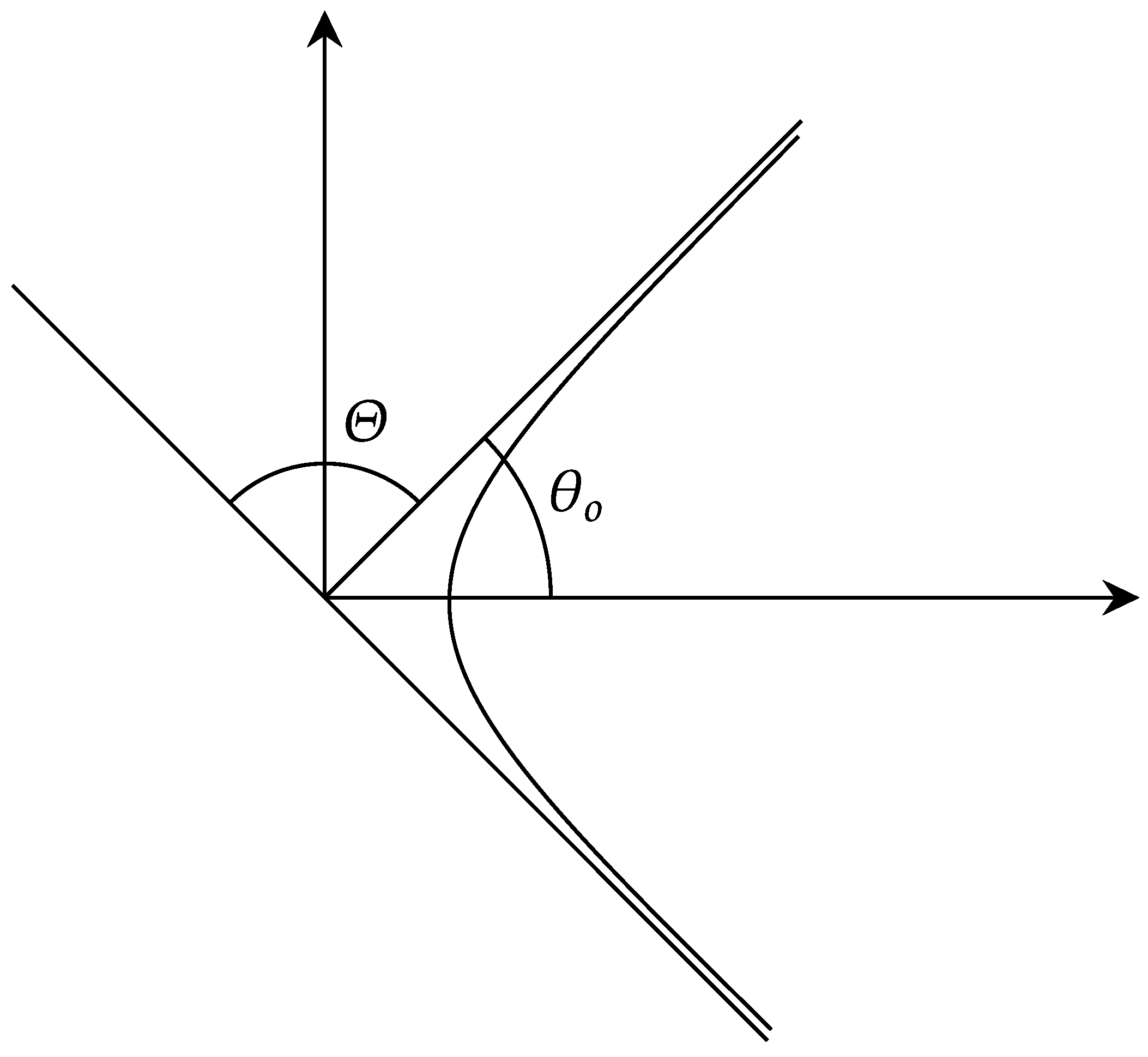
Figure 2.
Fixed point dispersion
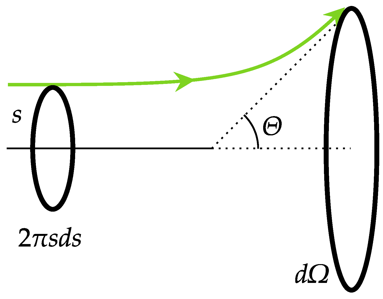
Figure 3.
Effective diameter of the electron in a plasma as a function of density and temperature. a in m, T in K and n in
Figure 3.
Effective diameter of the electron in a plasma as a function of density and temperature. a in m, T in K and n in
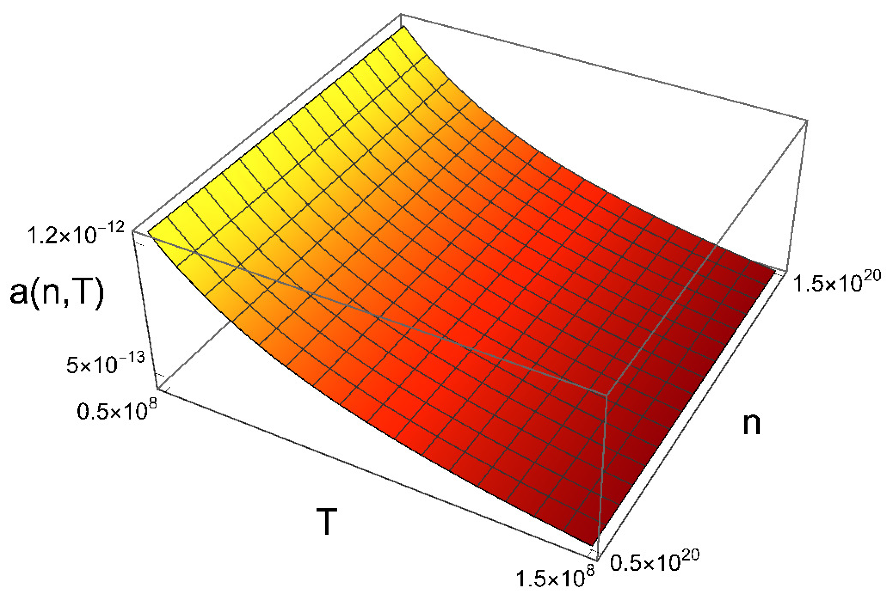
Figure 4.
The diameter "a" in m as function of T in K for fixed .
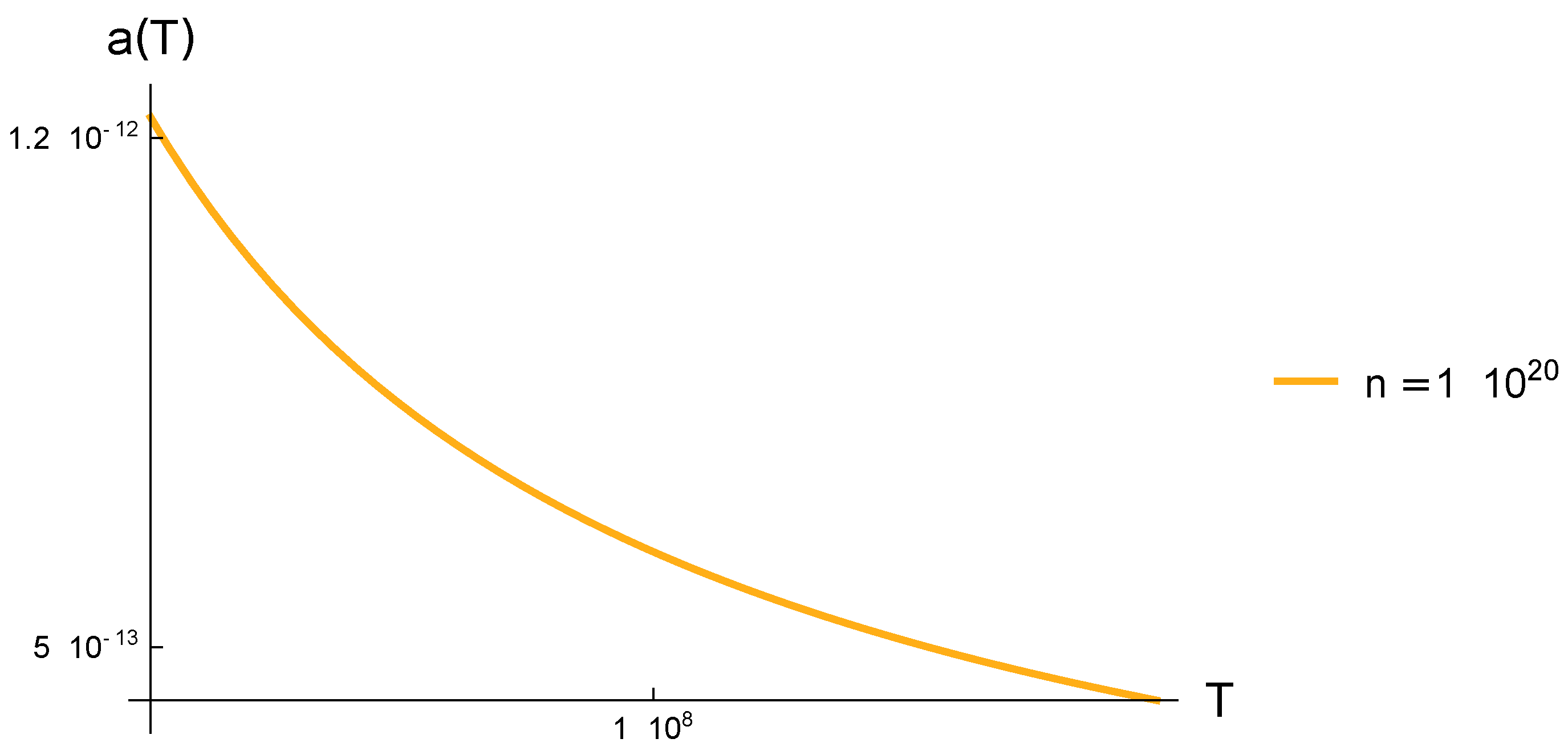
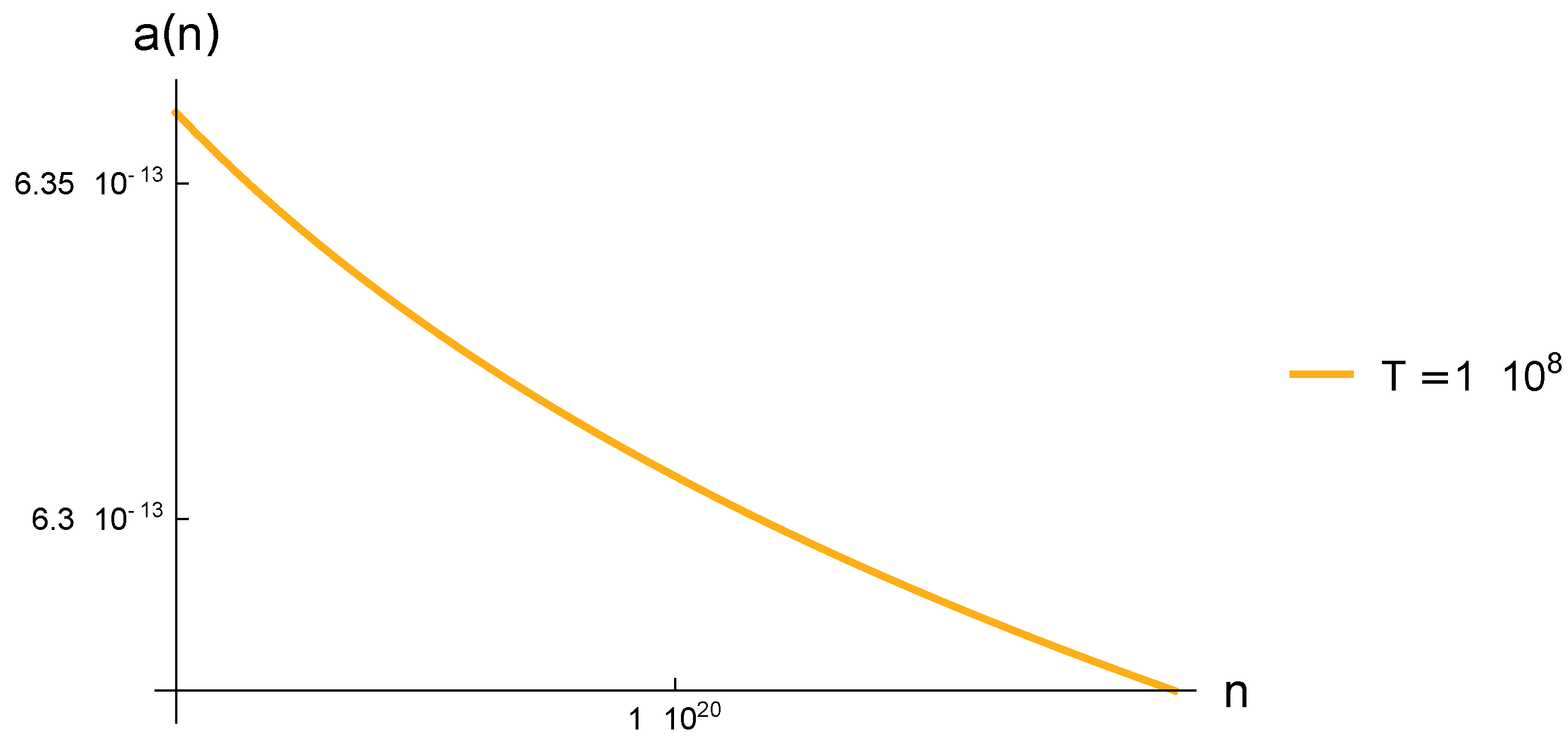
Figure 5.
The diameter "a" in m as function of n in for fixed temperature .
Disclaimer/Publisher’s Note: The statements, opinions and data contained in all publications are solely those of the individual author(s) and contributor(s) and not of MDPI and/or the editor(s). MDPI and/or the editor(s) disclaim responsibility for any injury to people or property resulting from any ideas, methods, instructions or products referred to in the content. |
© 2025 by the authors. Licensee MDPI, Basel, Switzerland. This article is an open access article distributed under the terms and conditions of the Creative Commons Attribution (CC BY) license (http://creativecommons.org/licenses/by/4.0/).
Copyright: This open access article is published under a Creative Commons CC BY 4.0 license, which permit the free download, distribution, and reuse, provided that the author and preprint are cited in any reuse.


