
Submitted:
15 April 2025
Posted:
15 April 2025
You are already at the latest version
Abstract
The electrically evoked compound action potential (ECAP) is a physiological signal that is important for clinicians to assess a patient's hearing. A clean ECAP can be used to estimate the patient’s auditory neural activity patterns and ECAP magnitude using the panoramic ECAP (PECAP) approach. However, noisy ECAPs can introduce significant errors in parameter estimation, especially at low signal-to-noise ratios (SNRs). To address this problem, a two-stage preprocessing denoising (TSPD) algorithm is developed. First, the ECAP matrix can be constructed using the forward-masking technique. Thus, the ECAP matrix can be viewed as an image for the first stage of noise reduction using the improved spatial median filter. Then, the denoised ECAP matrix can be expanded and rearranged into a vector for the second stage of noise reduction using the log-spectral amplitude (LSA) Wiener filter. Lastly, the enhanced ECAP vector is reconstructed to the ECAP matrix for aforementioned parameter estimation using PECAP. The results show that the proposed method, called PECAP-TSPD, improves the estimation of auditory neural activity patterns and ECAP magnitudes compared to those of the baseline (PECAP) and unprocessed ECAP signals in terms of the normalized root mean square error (RMSE).
Keywords:
electrically evoked compound action potential (ECAP)
; panoramic ECAP (PECAP)
; log-spectral amplitude (LSA)
; root mean square error (RMSE)
1. Introduction
The electrically evoked compound action potential (ECAP) is the combined response of auditory nerve fibers to electrical stimulation by a cochlear implant (CI) [1,2]. The ECAP is a critical signal for clinicians to evaluate the functionality of a patient's auditory nerve fibers after CI surgery [3,4]. In the absence of feedback from CI users, the ECAP model can be of great value to clinicians assessing the hearing performance of CI users [5,6]. ECAP amplitude can be computerized and estimated using temporal or spatial methods [7,8,9]. The ECAP matrix can be constructed by measuring the ECAPs generated by the different electrode positions of the masker and probe stimuli. Such a method is referred to as the forward-masking technique [10]. The panoramic ECAP (PECAP) method [11,12] in the literature has shown that using a clean ECAP matrix can approximate auditory activity patterns and ECAP magnitudes [11,12], further assisting clinicians in evaluating a patient's speech perception. Nevertheless, the use of noisy ECAP matrices, particularly when the signal-to-noise ratio (SNR) is less than 10 dB, has the potential to introduce inaccuracies in the estimation of auditory activity patterns and ECAP magnitudes [11,12].
The aforementioned reason necessitates the implementation of noise reduction techniques on ECAP matrices prior to estimating the auditory activity patterns and ECAP magnitudes. These techniques can be classified into three primary categories: spatial filtering, temporal filtering, and spectral filtering. In the context of image signal processing, the mean and median filters represent well-established examples of spatial filtering [13,14,15]. The mean filter is a linear estimator that is employed to mitigate the adverse effects of noise in images by eliminating random fluctuations. The principal disadvantage of the mean filter is that it results in image blurring, particularly at low SNRs. The median filter, which demonstrates superior noise removal performance in comparison to the mean filter, is a nonlinear estimator [16]. The median filter's masking size tends to increase with elevated noise levels, which can result in the loss of information from the original images. Thus, an improved median filtering algorithm (I-median) [17] is developed that combines the advantages of mean and median filters with the objective of achieving superior denoising in adverse environments. Specifically, if the current pixel is less than the average of the mask, the pixel is replaced with the median of the mask. Otherwise, the pixel keeps its original value [17].
In the field of time-domain signal analysis, adaptive filtering (AF) can be used to minimize noise. The AF method primarily uses algorithms such as least mean square (LMS) [18] and recursive least square (RLS) [19] to iteratively adjust the weights, thereby reducing the adverse effects of noise on the signal. The advantage of AF methods is its near real-time implementation [20]. However, a critical aspect of this method lies in the reference signal source, as clean signals, such as speech, are almost nonexistent in certain real-world scenarios. In addition, the choice of step size and filter order, which directly affect the rate of error convergence, is an important issue to address [21]. Finding the right balance is essential for noise reduction when AF is used.
Wiener filtering is an effective noise reduction technique in spectral domain signal analysis [22,23]. It operates by estimating the power spectral density (PSD) of the noise to enhance the signal. However, at low SNRs, the accuracy of the estimated noise PSD may decline, directly impacting noise reduction performance. To address this issue, a Wiener-based noise reduction algorithm known as log-spectral amplitude (LSA) Wiener filtering [24,25,26], has been developed to minimize the mean square error of the logarithmic spectrum. This approach helps alleviate the musical noise and improve the speech quality under low SNR conditions.
Recently, deep learning techniques have also been applied in the field of speech enhancement [27,28,29,30]. One such technique is the end-to-end convolutional recurrent neural network (CRN) [31], which enables near real-time implementation using a single microphone. This CRN algorithm can suppress noise under adverse conditions, such as a -5 dB SNR. However, the main drawback of these learning-based approaches is the substantial amount of data acquisition and preprocessing required [27,28,32], which can be both time- and resource- intensive. Additionally, the noise reduction performance may degrade when encountering unseen scenarios.
Given the compromised estimation of activation patterns and ECAP magnitudes using PECAP under low SNR conditions, this work proposes a method that combines PECAP with a two-stage preprocessing denoising algorithm (TSPD), referred to as PECAP-TSPD. Specifically, the ECAP signals are first denoised by TSPD and then used to estimate the neural parameters by PECAP. In the first stage of TSPD, the I-median algorithm is used to reduce the random noise of an ECAP matrix, since the ECAP matrix can be considered as an image. In the second step of TSPD, the denoised ECAP matrix is expanded and rearranged as a vector, where is the total number of electrodes. The rearranged vector can then be used as the input of the one-dimensional signal to LSA Wiener filtering for residual noise reduction. The PECAP-TSPD algorithm improves the accuracy of the estimates for key parameter, e.g., neural health and current spread. As a result, the refined approach leads to more reliable estimates of neural activation patterns and ECAP magnitudes, improving the effectiveness of neural assessments by clinicians. The normalized root mean square error (RMSE) serves as an objective measure in this work to evaluate the performance of the unprocessed data, PECAP-processed data, and PECAP-TSPD-processed data under various SNR conditions, densities, and scenarios. It also serves to highlight the accuracy of estimating ECAP magnitudes and activation patterns.
2. Panoramic ECAP Method
The panoramic ECAP (PECAP) method consists of two procedures: the forward-masking method and neural parameter estimation using sequential quadratic programming (SQP) [10,11,12]. The forward-masking method uses a probe and a masker to stimulate auditory neurons, generating the ECAP signal and reducing artifact. This process constructs a matrix in which each element represents the measured ECAP signal from each pair of probe and masker positions, as illustrated in Figure 1. In Figure 1, the x-axis represents the position of the masker, and the y-axis represents the position of the probe. Figure 1 shows the simulated ECAP signal, illustrating the inverse relationship between the amplitude of the ECAP and the distance from the probe to the masker. When the positions of the probe and the masker are closer, the amplitude of the ECAP signal is larger. Conversely, when the probe and masker are farther apart, the amplitude of the ECAP signal is smaller. This phenomenon can be explained in Figure 2 [6]. In Figure 2, the neural activity pattern is assumed to follow a Gaussian distribution. The ECAP signal can be regarded as the overlapping area between two Gaussian distributions, corresponding to the neural activity patterns stimulated by the probe and masker, respectively. The overlap is maximized when the positions of the probe and the masker coincide. In contrast, the overlap becomes minimal when the positions of the probe and the masker are distant from each other.
The auditory neural activity pattern is assumed to be a Gaussian distribution as follows:
where denotes the th electrode. denotes the total number of electrodes. is the position along the cochlea. Ideally, is a range from to . In this work, the range of is from to in which is set to , the total number of electrode. and are the auditory neuron amplitude and neural health of the th electrode, respectively. is an exponential function. and represent the mean and standard deviation (also referred to as current spread10 in physiological signals) of the Gaussian pattern for the th electrode, respectively. In this work, and is a prior information. Under an assumption that the ECAP signal is the overlap between the two auditory neuron responses of the probe and masker stimuli, the ECAP signal can be formulated as
where is the index indicating that the th electrode is stimulated by the probe. is the index indicating that the th electrode is stimulated by the masker. Equation (2) can also be expressed as a matrix form [12].
in which is an auditory neuron pattern matrix for each auditory neuron vector . Because is a symmetric matrix, the matrix of the ECAP signal in Equation (3) is also a symmetric matrix. The part of random noise can be alleviated using the following equation:
where represents the denoised matrix of the ECAP signal. To further estimate and , the SQP, a constrained optimization algorithm, is utilized. Computerization of the parameter estimation of the ECAP matrix is illustrated in Figure 3.
In Figure 3, , which denotes the normalized root mean square error between the measured and estimated ECAP matrices, is formulated as
where represents the maximum absolute value of Different SNR and density conditions are also introduced to assess the parameter estimation capability using SQP in this work.
Figure 4 depicts a structure designed to test the noise resistance performance using the SQP algorithm. The in Figure 3 and Figure 4 can be replaced by , as described in Equation (4) for random noise reduction. In addition, the normalized root mean square error between the ground truth and the estimated can be calculated, as shown in Equation (6).
where denotes the maximum absolute value of . After estimating the parameters of and , the denoised ECAP matrix can be reconstructed using Equation (3). The above procedures can eliminate most part of the noise. However, in low SNR scenarios, the distortion increases due to the error estimation of and . Therefore, the preprocessing algorithm is developed below.
3. Proposed Method
3.1. First Stage Noise Reduction Processing
In light of the detrimental effect of noise on the estimation of neural parameters, this work proposes a two-stage preprocessing denoising (TSPD) algorithm for the ECAP matrix, prior to the PECAP algorithm. First, the ECAP matrix is treated as an image. In the first stage of TSPD, the improved median filtering (I-median) algorithm is applied to reduce noise, as shown in Equation (7).
where and denote the processed values using the median and mean filters at the positions of , respectively. denotes the processed result using I-median. The masker sizes of median and mean filtering are set to in this work. Equation (7) describes that if the ECAP value at the positions is less than the mean filter processing value, the ECAP value is considered noise and can be replaced by the median filter processing value. Conversely, if the ECAP value is greater, it is retained. The processed ECAP matrix is expressed as
The I-Median algorithm is suitable for removing low to medium density noise from an image. In some cases, however, the noise is distributed across all pixels of an image. To further deal with this type of noise, and assuming that the ECAP signals are the overlaps between the probe and masker stimuli. This work expands into a vector in accordance with the following rule:
- 1.
- Calculate the absolute value of index minus indexwhere is an index matrix that records the absolute value of position difference between and
- 2.
- record for each element in and concatenate each row into a long vector.where
- 3.
- Conduct a descending order of and record the descending order index.where represents the descending order operation. is vector based on the descending order results of . is the index vector corresponding to .
- 4.
- The desired vector then can be obtained using the following equation:
By examining the ECAP signal in Figure 1 and Figure 2, the maximum can be reached when the probe and masker positions are close, and the minimum can be reached when the probe and masker positions are far apart. Therefore, in the previous steps, the noise (where ECAP signal is weak) would be placed in the first part of the vector. The target signal (where strong ECAP signal) can then be placed in the last part of the vector. The reordering processing is part of the second stage of TSPD, which employs log-spectral amplitude (LSA) Wiener filtering for improved noise reduction.
3.2. Second Stage Noise Reduction Processing
In the second stage of TSPD, LSA Wiener filtering is utilized to address the residual noise in the vector , which is treated as a discrete-time series input. The first step is to transform into a short-time Fourier transform (STFT) domain, as shown in Equation (13).
where is the STFT signal of . and denote the time frame and frequency indices, respectively. is the size of fast Fourier transform (FFT), is the hop size, and is the window for short-time signal analysis. is the th root of unity with . The LSA Wiener filter aims at minimizing the log-spectral amplitude
where is the cost function to minimize the mean square error of log-spectral amplitudes and . and are the clean signal and estimated clean signal spectrums, respectively. The optimal solution is
where is the prior SNR with being a clean signal PSD and being a residual noise PSD. with representing the posterior SNR. can be estimated using the decision-directed approach as described below:
where is a forgetting factor. can be estimated and updated using the following log-likelihood ratio criterion:
where
is the conditional probability density function (PDF) of given that the event () of the ECAP signal occurs.
is the conditional PDF of assuming only noise occurs at event . . If is less than a small value , the noise PSD can be updated using the following recursive averaging.
The estimated clean ECAP signal can be obtained using the following equation:
The complete LAS Wiener filtering procedures used in the second noise reduction stage are listed in Table 1.
In Table 1, is the number of time frames used to represent the presence of noise. Next, the processed row vector is conversed into using the inverse STFT the time domain signal which can be reconstructed into the matrix format, as described below:
where is defined in Equation (11) with being a range of to In this work, the mean filter is applied in if the SNR value is below 4 dB, in order to leverage the advantage of random noise removal at low SNRs [15].
4. Settings and Results
Two types of noise – random noise and impulse noise – are used to evaluate the performance of the proposed PECAP-TSPD algorithm. Twelve SNR levels, -5 dB, -2 dB, 1 dB, 4 dB, 7 dB, 10 dB, 13 dB, 16 dB, 19 dB, 22 dB, 25 dB, and 100 dB (representing the clean ECAP signal situation for random noise case) are used in the random noise. Four densities, 10%, 20%, 30%, and 40%, are used in the impulse noise. Normalized RMSE is used as an objective quality measure to calculate the error between the ground truth and the estimated results (neural health and ECAP amplitude). Seven different combinations of neural health and current spread are listed in Table 2. The results of the ECAP matrices before and after processing at -5 dB of SNR are shown in Figure 5.
In Figure 5(b), the ECAP matrix is filled with random noise, thereby, making it difficult to observe the pristine measured ECAP data, as depicted in Figure 5(a). The PECAP and PECAP-TSPD methods can mitigate the detrimental effects of extremely noisy environments to recover the clean ECAP matrix shown in Figure 5(c) and (d). The images of Figure. 5(a) and (d) are almost identical, further presenting the satisfactory performance of PECAP-TSPD. The results of the normalized RMSE of the ECAP magnitude () and neural activity pattern () are depicted in Figure 6.
Figure 6(a) shows the normalized RMSE of the unprocessed ECAP signals, ECAP signals processed by PECAP and PECAP-TSPD algorithms for different SNRs in Scenario 1. The normalized RMSE of the magnitude of the unprocessed ECAP signals at -5 dB SNR increases to 83.39%, which is comparably higher than those of the processed ECAP signals by PECAP (16.17%) and PECAP-TSPD (5.23%), indicating the need for ECAP signal processing. When comparing the between PECAP and PECAP-TSPD processing ECAP signals, the values of by PECAP-TSPD are all smaller than those by PECAP except the 100 dB SNR case, where are and for PECAP and PECAP-TSPD, respectively. Figure 6(b) presents the curve of the average normalized RMSE, which is formulated as follows for each scenario:
where represents the total number of SNR conditions in this work. and represent each index () value of each SNR condition () in the pristine and estimated ECAP matrices, respectively. is the maximum absolute value of which denotes the pristine ECAP matrix of each SNR condition. Similar to , is described as
in which and denote each index value of each SNR condition in the pristine and estimated neural activity patterns, respectively. is the maximum absolute value of which denotes the pristine neural activity pattern of each SNR condition. Compared to the unprocessed and processed ECAP signals, the maximum values of are 6.17% and 5.48% for PECAP and PECAP-TSPD, respectively. In contrast, the maximum value of the unprocessed ECAP signals is 28.97% for , showing that the noise resistance capability of the PECAP and PECAP-TSPD algorithms. The performance of the PECAP-TSPD algorithm is superior to that of the PECAP algorithm, as the values of and obtained with PECAP-TSPD are lower than those obtained with PECAP. The average of from Scenarios 1 to 7 can be ranked as: PECAP-TSPD (3.83%), PECAP (5.14%), and unprocessed (23.07%). The averages of from Scenarios 1 to 7 for PECAP-TSPD and PECAP are 3.01% and 4.64%, respectively.
Next, the impulse noise is added into the EACP matrix to evaluate the performance of PECAP-TSPD under four different densities. Figure 7 illustrates the results of the ECAP matrices before and after using the PECAP and PECAP-TSPD algorithms at the 40% density of the impulse noise.
The impulse noise with 40% density heavily contaminates the original ECAP matrix (Figure 7(a)), as shown in Figure 7(b), emphasizing the importance of signal processing. The processed ECAP matrices using the PECAP and PECAP-TSPD algorithms are depicted in Figure 7(c) and (d), where the impulse noise is most reduced. When comparing Figure 7(c) to Figure 7(d), the restored ECAP matrix in Figure 7(d) shows more resemblance to Figure 7(a) than to that of Figure 7(c), exhibiting the satisfactory performance of PECAP-TSPD under adverse noisy environments. The normalized RMSE results of the ECAP magnitude and neural activity pattern of the impulse noise case are depicted in Figure 8.
Figure 8(a) presents the and curves at four distinct densities in Scenario 2 for the unprocessed, PECAP, and PECAP-TSPD approaches, all of which increase as the impulse noise density increases. In the case of 40% impulse noise density, the values for unprocessed, PECAP, and PECAP-TSPD are 34.07%, 8.44%, and 2.96%, respectively, displaying the effectiveness of PECAP and PECAP-TSPD in highly noisy environments. The average normalized RMSE results are depicted in Figure 6(b), in which and are similar to Eqs. (23) and (24), except that is replaced by , denoting the total number of impulse noise densities in this work. The maximum value of for the PECAP and PECAP-TSPD algorithms is 6.77% and 4.22%, respectively. For the unprocessed ECAP matrices, the maximum value of is 27.59%, which suggests that PECAP and PECAP-TSPD are robust against noise. The PECAP-TSPD algorithm performs better than the PECAP algorithm because the values of and calculated by PECAP-TSPD are lower than those calculated by PECAP. The mean values of from Scenarios 1 through 7 can be arranged in ascending order as follows: PECAP-TSPD (3.13%), PECAP (5.57%), and unprocessed (21.97%). The mean values of from Scenarios 1 to 7 for PECAP-TSPD and PECAP are 2.39% and 5.23%, respectively.
5. Conclusions
The PECAP-TSPD algorithm, which integrates the improved median filter, the log-spectral Wiener filter, and PECAP, has been developed for noise reduction in ECAP data to accurately estimate neural health and current spread from severely noisy ECAP matrices. The normalized RMSE for ECAP magnitude () and neural activity pattern () demonstrates that both the PECAP and PECAP-TSPD algorithms effectively reduce and compared to unprocessed data under various SNRs, noise densities, and experimental scenarios. Notably, PECAP-TSPD outperforms PECAP in terms of both and . For ECAP matrices corrupted by random noise, the average across seven different scenarios and twelve SNR levels is as follows: PECAP-TSPD (3.83%), PECAP (5.14%), and unprocessed (23.07%). In the case of impulse noise, the ranking is: PECAP-TSPD (3.13%), PECAP (5.57%), and unprocessed (21.97%). Similarly, the average for PECAP-TSPD and PECAP under random noise conditions are 3.01% and 4.64%, respectively. Under impulse noise, the values are 2.39% for PECAP-TSPD and 5.23% for PECAP.
Author Contributions
Author Fan-Jie Kung designs the PECAP-TSPD algorithm, finishes the program, and writes this article.
Funding
This research was funded by the National Science and Technology Council (NSTC) of Taiwan, grant number 113-2222-E-027-010- and the APC was funded by 113-2222-E-027-010-.
Data Availability Statement
The data that support the findings of this study are available from the corresponding author upon reasonable request.
Acknowledgments
Author Fan-Jie Kung appreciates valuable comments from reviewers to improve this article.
Conflicts of Interest
Author Fan-Jie Kung has no conflicts to disclose.
Abbreviations
The following abbreviations are used in this manuscript:
| ECAP | Electrically evoked compound action potential |
| PECAP | Panoramic ECAP |
| SNR | Signal-to-noise ratio |
| TSPD | Two-stage preprocessing denoising algorithm |
| LSA | Log-spectral amplitude |
| RMSE | Root mean square error |
| Unpro | Unprocessed data |
References
- Liebscher, T.; Hornung, J.; Hoppe, U. Electrically evoked compound action potentials in cochlear implant users with preoperative residual hearing. Front. Hum. Neurosci. 2023, 17, 1125747. [Google Scholar] [CrossRef]
- He, S.; Teagle, H.F.B.; Buchman, C.A. The Electrically Evoked Compound Action Potential: From Laboratory to Clinic. Front. Neurosci. 2017, 11, 339–339. [Google Scholar] [CrossRef]
- Hughes, M. L. Fundamentals of Clinical ECAP Measures in Cochlear Implants: Part 1: Use of the ECAP in Speech Processor Programming (2nd Ed.) (accessed on 13 February, 2025).
- DeVries, L.; Scheperle, R.; Bierer, J.A. Assessing the Electrode-Neuron Interface with the Electrically Evoked Compound Action Potential, Electrode Position, and Behavioral Thresholds. J. Assoc. Res. Otolaryngol. 2016, 17, 237–252. [Google Scholar] [CrossRef] [PubMed]
- Choi, C.T.M.; Wu, D.L. Electrically Evoked Compound Action Potential Studies Based on Finite Element and Neuron Models. IEEE Trans. Magn. 2022, 58, 1–4. [Google Scholar] [CrossRef]
- Garcia, C.; Goehring, T.; Cosentino, S.; Turner, R.E.; Deeks, J.M.; Brochier, T.; Rughooputh, T.; Bance, M.; Carlyon, R.P. The Panoramic ECAP Method: Estimating Patient-Specific Patterns of Current Spread and Neural Health in Cochlear Implant Users. J. Assoc. Res. Otolaryngol. 2021, 22, 567–589. [Google Scholar] [CrossRef] [PubMed]
- Dong, Y.; Briaire, J.J.; Stronks, H.C.; Frijns, J.H.M. Speech Perception Performance in Cochlear Implant Recipients Correlates to the Number and Synchrony of Excited Auditory Nerve Fibers Derived From Electrically Evoked Compound Action Potentials. Ear Hear. 2022, 44, 276–286. [Google Scholar] [CrossRef]
- Takanen, M.; Strahl, S.; Schwarz, K. Insights Into Electrophysiological Metrics of Cochlear Health in Cochlear Implant Users Using a Computational Model. J. Assoc. Res. Otolaryngol. 2024, 25, 63–78. [Google Scholar] [CrossRef]
- Takanen, M.; Seeber, B.U. A Phenomenological Model Reproducing Temporal Response Characteristics of an Electrically Stimulated Auditory Nerve Fiber. Trends Hear. 2022, 26. [Google Scholar] [CrossRef]
- Garcia, C.; Deeks, J.M.; Goehring, T.; Borsetto, D.; Bance, M.; Carlyon, R.P. SpeedCAP: An Efficient Method for Estimating Neural Activation Patterns Using Electrically Evoked Compound Action-Potentials in Cochlear Implant Users. Ear Hear. 2022, 44, 627–640. [Google Scholar] [CrossRef]
- Cosentino, S.; Gaudrain, E.; Deeks, J.M.; Carlyon, R.P. Multistage nonlinear optimization to recover neural activation patterns from evoked compound action potentials of cochlear implant users. IEEE Trans. Biomed. Eng. 2015, 63, 1–1. [Google Scholar] [CrossRef]
- Garcia, C.; Goehring, T.; Cosentino, S.; Turner, R.E.; Deeks, J.M.; Brochier, T.; Rughooputh, T.; Bance, M.; Carlyon, R.P. The Panoramic ECAP Method: Estimating Patient-Specific Patterns of Current Spread and Neural Health in Cochlear Implant Users. J. Assoc. Res. Otolaryngol. 2021, 22, 567–589. [Google Scholar] [CrossRef]
- Isnanto, R.R.; Windarto, Y.E.; Mangkuratmaja, M.V. Assessment on Image Quality Changes as a Result of Implementing Median Filtering, Wiener Filtering, Histogram Equalization, and Hybrid Methods on Noisy Images. 2020 7th International Conference on Information Technology, Computer, and Electrical Engineering (ICITACEE). LOCATION OF CONFERENCE, IndonesiaDATE OF CONFERENCE; pp. 185–190.
- Gupta, G. Algorithm for image processing using improved median filter and comparison of mean, median and improved median filter. International Journal of Soft Computing and Engineering 2011, 1, 304–311 [CrossRef]. [Google Scholar]
- Sun, M. Comparison of processing results of median filter and mean filter on Gaussian noise. Appl. Comput. Eng. 2023, 5, 779–785. [Google Scholar] [CrossRef]
- Hou, Y.; Li, Q.; Zhang, C.; Lu, G.; Ye, Z.; Chen, Y.; Wang, L.; Cao, D. The State-of-the-Art Review on Applications of Intrusive Sensing, Image Processing Techniques, and Machine Learning Methods in Pavement Monitoring and Analysis. Engineering 2021, 7, 845–856. [Google Scholar] [CrossRef]
- Zhu, Y.; Huang, C. An Improved Median Filtering Algorithm for Image Noise Reduction. Phys. Procedia 2012, 25, 609–616. [Google Scholar] [CrossRef]
- Jiang, D. A study on adaptive filtering for noise and echo cancellation. Master’s thesis, University of Windsor, 2005.
- Yazdanpanah, H.; Diniz, P. S. R. Recursive least-squares algorithms for sparse system modeling. In Proceedings of the IEEE International Conference on Acoustics, Speech and Signal Processing, New Orleans, LA, USA, 2017. [CrossRef], 5-9 March.
- Creighton, J.; Doraiswami, R. Real time implementation of an adaptive filter for speech enhancement. In Proceedings of the Canadian Conference on Electrical and Computer Engineering, Niagara Falls, ON, Canada, 2004. [CrossRef], 2-5 May.
- Wang, P.; Kam, P.-Y. An automatic step-size adjustment algorithm for LMS adaptive filters, and an application to channel estimation. Phys. Commun. 2012, 5, 280–286. [Google Scholar] [CrossRef]
- Loizou, P. C. Speech Enhancement: Theory and Practice, 1st ed.; CRC Press: New York, USA, 2007; pp. 143–208. [Google Scholar]
- Benesty, J.; Chen, J.; Huang, Y. Microphone Array Signal Processing, Springer: Verlag Berlin Heidelberg, Germany, 2008; pp. 8–15.
- Ephraim, Y.; Malah, D. Speech enhancement using a minimum mean-square error log-spectral amplitude estimator. IEEE Trans. Acoust. Speech, Signal Process. 1985, 33, 443–445. [Google Scholar] [CrossRef]
- Borgstrom, B.J.; Alwan, A. Log-spectral amplitude estimation with Generalized Gamma distributions for speech enhancement. ICASSP 2011 - 2011 IEEE International Conference on Acoustics, Speech and Signal Processing (ICASSP). LOCATION OF CONFERENCE, Czech RepublicDATE OF CONFERENCE; pp. 4756–4759.
- Hirszhorn, A.; Dov, D.; Talmon, R.; Cohen, I. Transient interference suppression in speech signals based on the OM-LSA algorithm. In Proceedings of the International Workshop on Acoustic Echo and Noise Control, Aachen, Germany, 2012. [CrossRef], 4-6 September 4-6.
- Hsu, Y.; Bai, M.R. Learning-based robust speaker counting and separation with the aid of spatial coherence. EURASIP J. Audio, Speech, Music. Process. 2023, 2023, 1–21. [Google Scholar] [CrossRef]
- Hsu, Y.; Lee, Y.; Bai, M.R. Array configuration-agnostic personalized speech enhancement using long-short-term spatial coherence. J. Acoust. Soc. Am. 2023, 154, 2499–2511. [Google Scholar] [CrossRef]
- Richard, G.; Smaragdis, P.; Gannot, S.; Naylor, P.A.; Makino, S.; Kellermann, W.; Sugiyama, A. Audio Signal Processing in the 21st Century: The important outcomes of the past 25 years. IEEE Signal Process. Mag. 2023, 40, 12–26. [Google Scholar] [CrossRef]
- Gannot, S.; Tan, Z.-H.; Haardt, M.; Chen, N.F.; Wai, H.-T.; Tashev, I.; Kellermann, W.; Dauwels, J. Data Science Education: The Signal Processing Perspective [SP Education]. IEEE Signal Process. Mag. 2023, 40, 89–93. [Google Scholar] [CrossRef]
- Tan, K.; Wang, D. A Convolutional Recurrent Neural Network for Real-Time Speech Enhancement. Interspeech 2018. LOCATION OF CONFERENCE, COUNTRYDATE OF CONFERENCE;
- Bianco, M.J.; Gerstoft, P.; Traer, J.; Ozanich, E.; Roch, M.A.; Gannot, S.; Deledalle, C.-A. Machine learning in acoustics: Theory and applications. J. Acoust. Soc. Am. 2019, 146, 3590–3628. [Google Scholar] [CrossRef] [PubMed]
Figure 1.
An illustration of an ECAP matrix simulation. The x-axis represents the position of the masker (from Electrode 22 to Electrode 1), and the y-axis represents the position of the probe (from Electrode 1 to Electrode 22) [12].
Figure 1.
An illustration of an ECAP matrix simulation. The x-axis represents the position of the masker (from Electrode 22 to Electrode 1), and the y-axis represents the position of the probe (from Electrode 1 to Electrode 22) [12].
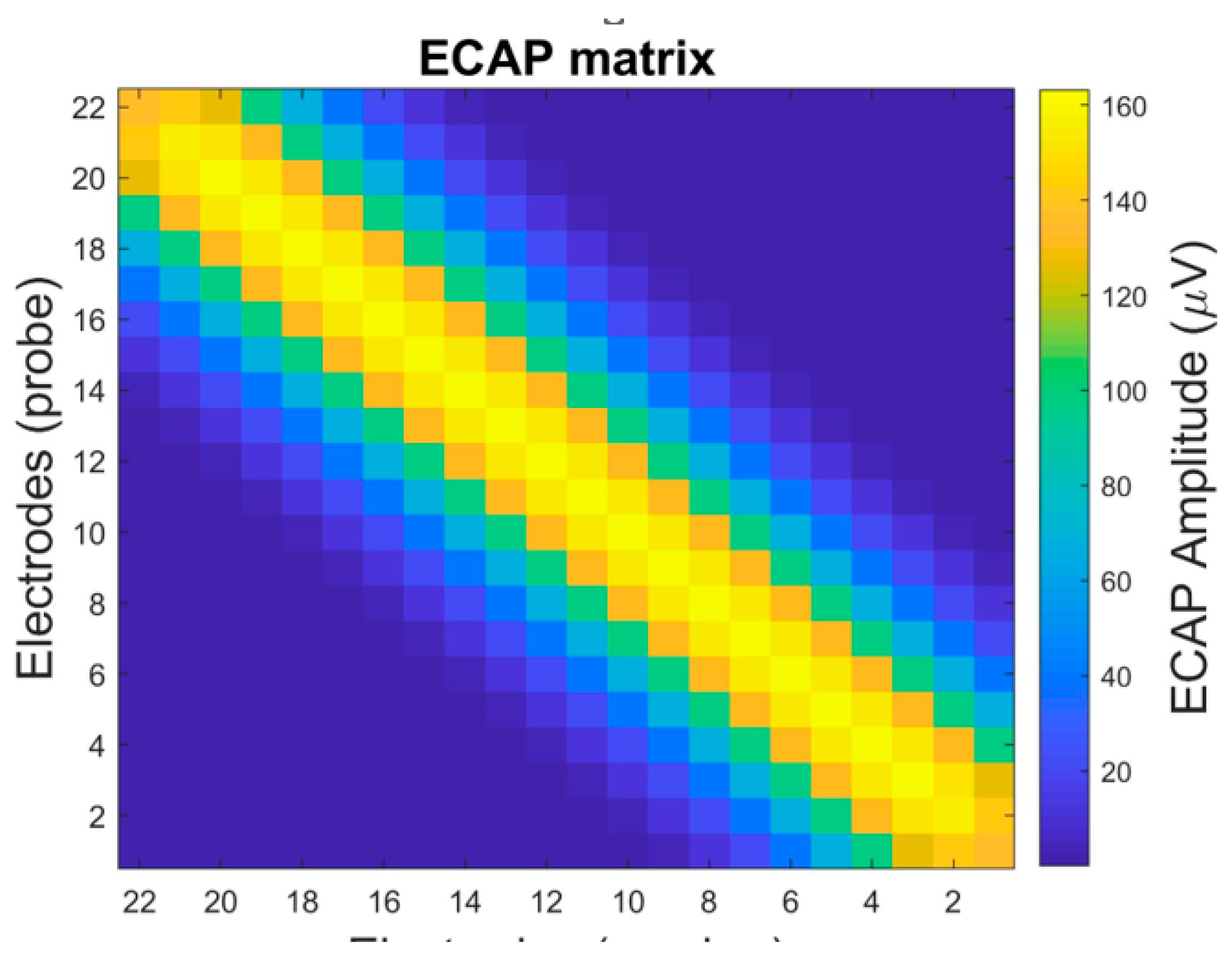
Figure 2.
Schematic illustrating the overlapping area stimulated by the probe and the masker. Gaussian distributions represent the auditory neuron response, and the shaded overlapping indicates the ECAP response [6].
Figure 2.
Schematic illustrating the overlapping area stimulated by the probe and the masker. Gaussian distributions represent the auditory neuron response, and the shaded overlapping indicates the ECAP response [6].
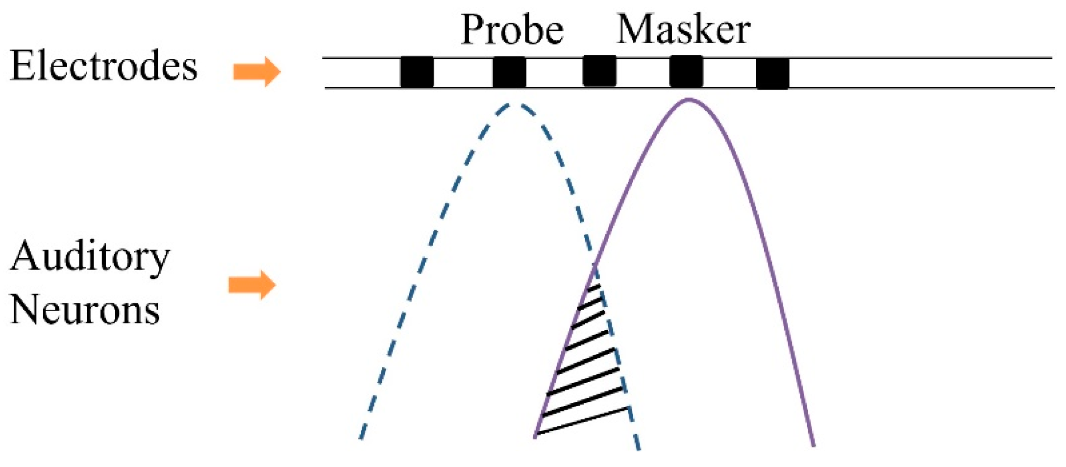
Figure 3.
The block diagram of neural parameter estimation in the ECAP matrix using the SQP algorithm [6,12].
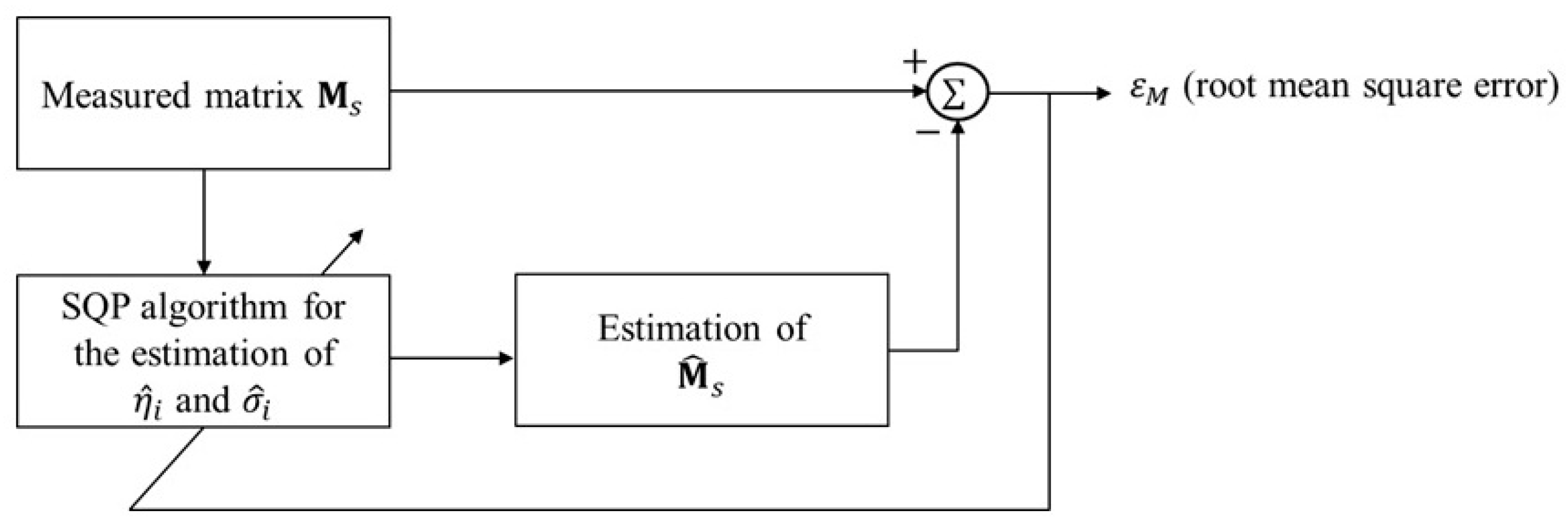
Figure 4.
The block diagram of parameter estimation with additive noise scenarios using the SQP algorithm [11,12].
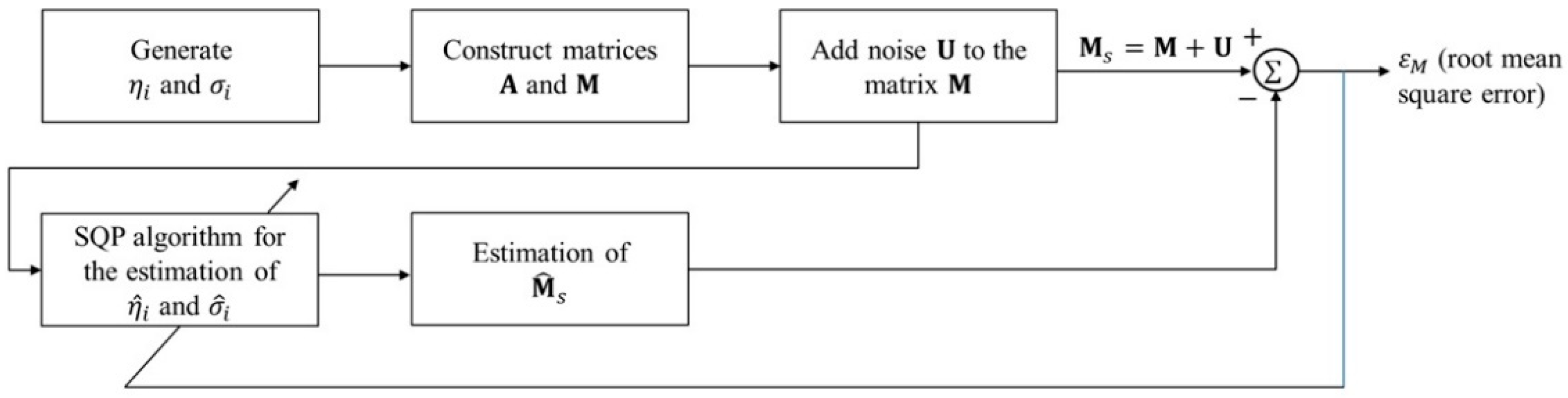
Figure 5.
The results of (a) ECAP matrix at 100 dB SNR, (b) noisy ECAP matrix at -5 dB SNR, (c) processed ECAP matrix using the PECAP method at -5 dB SNR, and (d) processed ECAP matrix using the TSPD method at -5 dB. The neural health and current spread settings are scenario 1 listed in Table 2.
Figure 5.
The results of (a) ECAP matrix at 100 dB SNR, (b) noisy ECAP matrix at -5 dB SNR, (c) processed ECAP matrix using the PECAP method at -5 dB SNR, and (d) processed ECAP matrix using the TSPD method at -5 dB. The neural health and current spread settings are scenario 1 listed in Table 2.
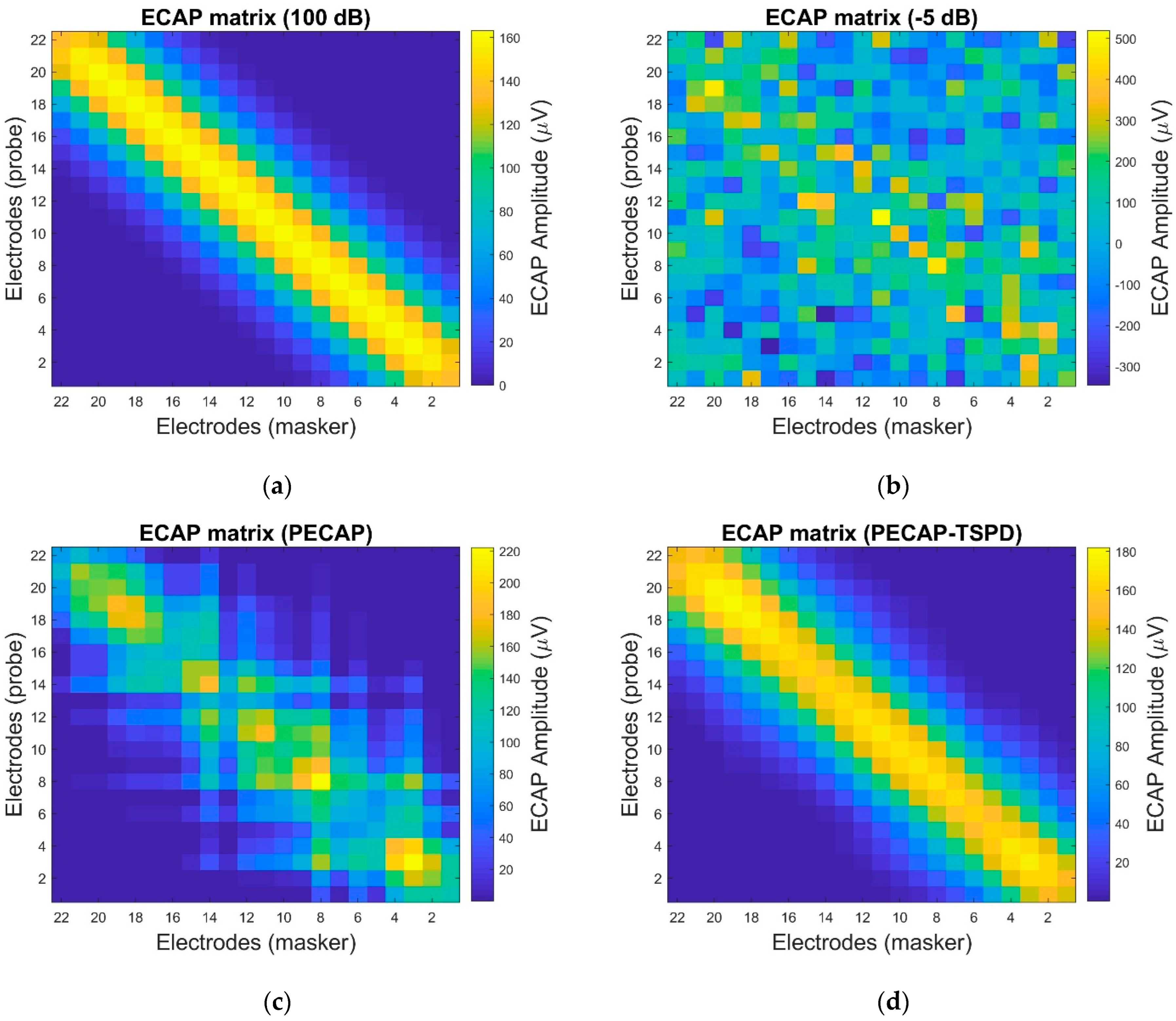
Figure 6.
The normalized RMSE and average normalized RMSE results of ECAP magnitudes and neural activity patterns under twelve SNR conditions (a) in scenario 1 and (b) in scenarios 1 to 7, respectively. The unprocessed ECAP matrices are used for comparison with the baseline PECAP and proposed PECAP-TSPD methods. The parameter settings for each scenario are shown in Table 2.
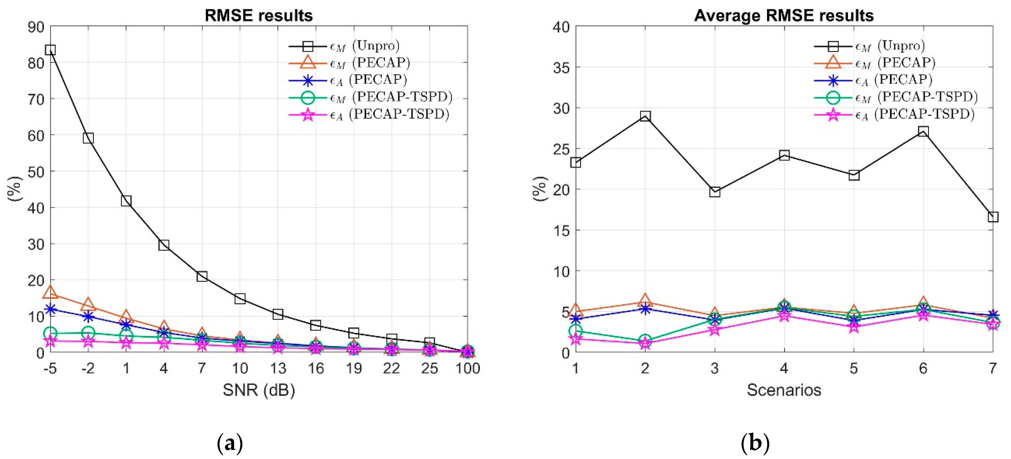
Figure 7.
The ECAP matrix results of (a) non-density impulse noise, (b) impulse noise of 40% density, (c) processed ECAP matrix using the PECAP method under 40% density impulse noise, and (d) processed ECAP matrix using the PECAP-TSPD method under 40% density impulse noise. The settings of neural health and current spread are scenario 2 listed in Table 2.
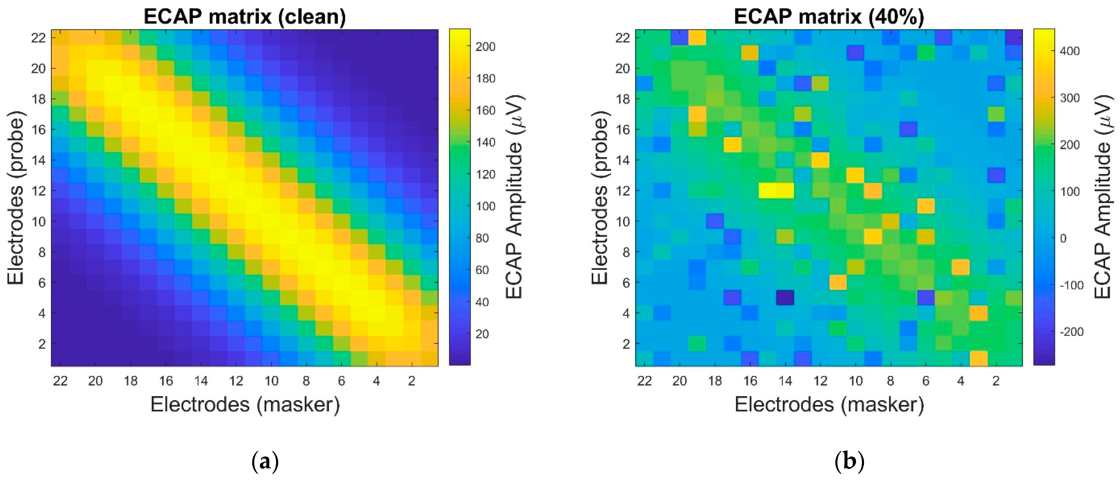
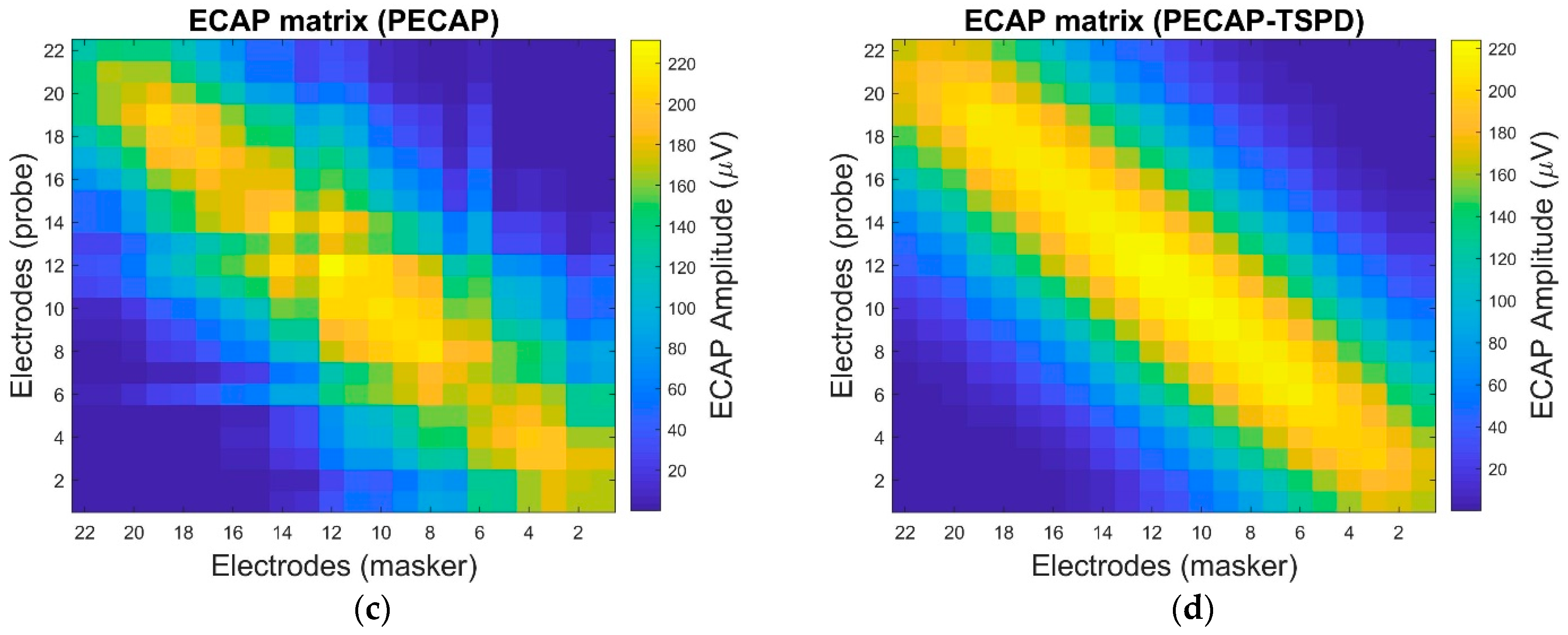
Figure 8.
The normalized RMSE and average normalized RMSE results of ECAP magnitudes and neural activity patterns under four impulse noise densities (a) in scenario 2 and (b) in scenarios 1 to 7, respectively. The unprocessed ECAP matrices are compared with the PECAP and PECAP-TSPD algorithms. The settings for each scenario are listed in Table 2.
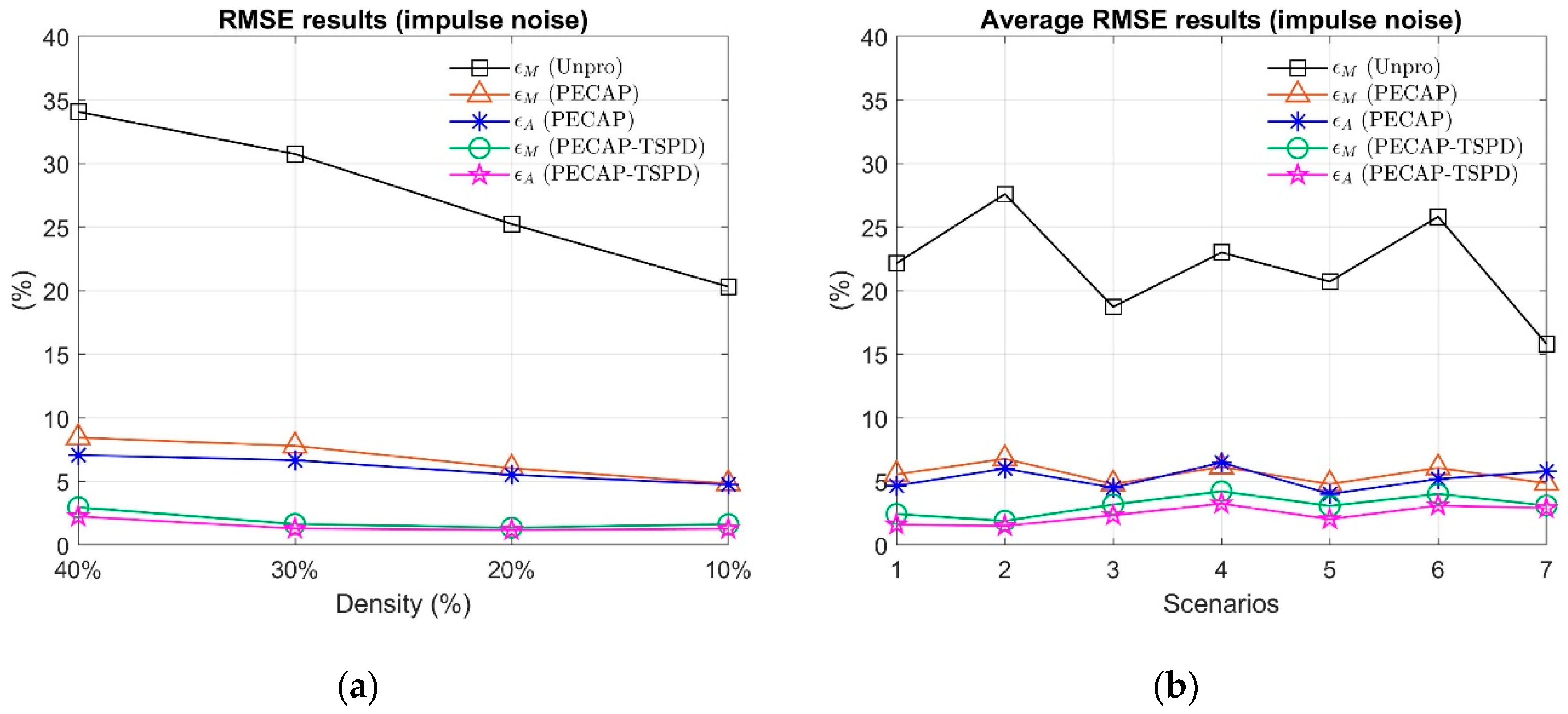

Table 1.
Steps involved in the LSA Wiener filtering algorithm.
| Step 1. Initialization of for each frequency bin For each and : Step 2. Estimation of If , then , else Step 3. Estimation of using Equation (16) If , then Equation (16) can be rewritten as Step 4. check the VAD criterion If , then using Equation (20) for updating Step 5. Calculation of using Equation (15) Step 6. Calculation of using Equation (21) End for |
Table 2.
Table 2. Different settings of neural health and current spread.
|
Scenario 1: , , , where in this study. Scenario 2: , , . Scenario 3: , . , , , . , . Scenario 4: , . , , , . , . Scenario 5: , . , , , . , . Scenario 6: , . , , , . , . Scenario 7: , . , , , , , , |
Disclaimer/Publisher’s Note: The statements, opinions and data contained in all publications are solely those of the individual author(s) and contributor(s) and not of MDPI and/or the editor(s). MDPI and/or the editor(s) disclaim responsibility for any injury to people or property resulting from any ideas, methods, instructions or products referred to in the content. |
© 2025 by the authors. Licensee MDPI, Basel, Switzerland. This article is an open access article distributed under the terms and conditions of the Creative Commons Attribution (CC BY) license (http://creativecommons.org/licenses/by/4.0/).
Copyright: This open access article is published under a Creative Commons CC BY 4.0 license, which permit the free download, distribution, and reuse, provided that the author and preprint are cited in any reuse.


