Submitted:
15 April 2025
Posted:
15 April 2025
You are already at the latest version
Abstract
This paper presents a neural network-based path planning method for fixed-wing UAVs under terminal roll angle constraints. The nonlinear optimal path planning problem is first formulated as an optimal control problem. The necessary conditions derived from Pontryagin’s Maximum Principle are then established to convert extremal trajectories as the solutions of a parameterized system. Additionally, a sufficient condition is proposed to guarantee that the obtained solution is at least locally optimal. By simply propagating the parameterized system, a training dataset comprising at least locally optimal trajectories can be constructed. A neural network is then trained to generate the nonlinear optimal control command in real time. Finally, numerical examples demonstrate that the proposed method robustly ensures the generation of at least local optimal trajectories in real time while satisfying the prescribed terminal roll angle constraint.
Keywords:
fixed-wing uav
; neural network
; path planning
; pontryagin’s maximum principle
; parameterized system
1. Introduction
Fixed-Wing Unmanned Aerial Vehicles (UAVs) is now playing a vital role in complex scenarios such as intelligence [1], surveillance [2], and reconnaissance [3]. To effectively perform these tasks, a UAV must have the ability of autonomously navigating itself to a desired target while satisfying various constraints. Path planning is a key aspect for a UAV to achieve such autonomy, which involves generating feasible paths from an initial position to an expected target position. Current UAV path planning methods can generally be classified into four categories: path-following methods, waypoint based methods, optimization based methods, and neural network based methods.
Path-following methods rely on designing tracking control law so that a UAV can be guided to accurately track a predefined path [4,5]. In [6,7,8], by considering a virtual target moving along the predefined path some Light-of-Sight (LOS) based methods have been developed to control the UAV to continuously move around the predefined path. Furthermore, a nonlinear adaptive LOS path-following controller was proposed by Cui et al. [7] via integrating an adaptive control scheme and sideslip compensation into the traditional LOS guidance law. Nelson et al [9] propose a vector-field based path following method, whose main idea is to construct a vector field in the vicinity of the desired path. A natural extension is presented in [10] by proposing a Gradient Vector Field (GVF) which involves tuning the some parameters according to the dynamics of UAV to achieve better performance. It should be noted that path-following methods are easy to implement. However, if the external environment changes, the UAV moves along the predefined paths may not complete its missions.
Waypoint-based methods involve defining a sequence of points (waypoints) and guiding a UAV to navigate between waypoints so that it can reach the target location. In the framework of waypoint-based methods, algorithms such as Dijkstra’s algorithm [11], roadmaps [12], Rapidly-exploring Random Trees (RRT) [13,14], have been extensively studied to find feasible paths. Specifically, Wang et al. [11] introduced an Elevation-based Dijkstra Algorithm (EDA) that leverages terrain elevation information to discretize the trajectory from the starting point to the target point into a series of straight-line segments. Compared with the traditional Dijkstra algorithm, the EDA exhibits superior computational efficiency. Xu et al. [15] introduced a Dubins-A* algorithm, which integrates Dubins path properties into the well-known A* algorithm to ensure both optimality and adherence to turning constraints, thereby demonstrating improved performance in environments with irregular obstacles. However, waypoint-based methods often neglect the dynamics of UAVs, which may lead to infeasible trajectories or necessitate subsequent curvature adjustments and smoothing processes to ensure physical feasibility [16].
Optimization-based methods cast path planning as an optimal control problem. By using Pontryagin’s Maximum Principle (PMP), a criterion (e.g. time or energy) is optimized while satisfying the dynamics of the UAVs [17,18]. De Marinis et al. [19] developed a minimum-time path planning method capable of avoiding obstacles by integrating classical optimal control theory with continuation methods. Forkan et al. [20] presented an approach for computing the shortest path to visit multiple target points while maintaining a minimum turning radius constraint, this method employs PMP to establish necessary optimality conditions and uses an arc parameterization technique to determine the ideal sequence of turns and straight segments. Additionally, Na et al. [21] introduced a path planning approach utilizing an enhanced Particle Swarm Optimization (PSO) algorithm, with the goal of optimizing the energy efficiency of fixed-wing UAVs when flying over mountainous regions. These methods can guarantee to generate optimal paths while accommodating complex constraints. However, they often require solving two-point boundary value problems [22] or performing exhaustive searches over trajectory families [23], leading to a significant computational burden for optimization-based planners [24].
Path planning methods based on neural networks can be categorized into supervised learning and Deep Reinforcement Learning (DRL). Supervised learning involves offline generation of a large amount of optimal trajectories and training a neural networks to approximate the mapping from state to control commands. Horn et al. [25] developed a trajectory optimization method that converts traditional collocation-point constraints into an offline training challenge, thereby significantly reducing online computational demands. However, despite employing the Sparse Nonlinear OPTimizer (SNOPT) [26] to efficiently generate training data, this approach cannot guarantee the solutions to be at least locally optimal, potentially affecting the learning performance of neural network. Phillips et al. [27] presented an approach that utilizes a lightweight Multi-Layer Perceptron (MLP) to estimate the cost of the nearest neighbor path, facilitating real-time prediction of the optimal path length for fixed-wing UAVs under wind disturbances. Since supervised learning only requires executing a single forward computation of the neural network during inference, making it ideal for scenarios with stringent real-time demands. However, supervised learning strongly relies on the quality and diversity of the training data [28].
DRL enables UAVs to autonomously learn optimal or near-optimal flight path planning strategies through trial-and-error and reward mechanisms [29]. For instance, Li et al. [30] proposed an algorithm that integrates DRL with adaptive control strategies. Babel [31] employs Deep Q-Networks (DQN) for online decision-making of fixed-wing UAVs in dynamic environments, enabling adaptive avoidance of sudden obstacles. Compared with traditional re-planning algorithms, its average computational cost is substantially reduced. Ji and Wang [32] incorporate energy consumption into the reward function of DRL, and throug extensive simulation training, propose a strategy that comprehensively optimizes speed, heading, and roll angle. Although DRL exhibits remarkable adaptability in complex environments and uncertain conditions, it demands a large amount of interactive data for training. Additionally, its convergence speed and stability are greatly influenced by the choice of algorithm and hyperparameter settings [5].
Motivated by these developments, this paper introduces a neural network-driven path-planning framework for fixed-wing UAVs that integrates optimal control principles to satisfy mission constraints in real time. A particularly challenging aspect of path planning for fixed-wing UAVs is satisfying terminal roll-angle constraints. In various missions, such as reconnaissance and formation, achieving a specified terminal roll angle is crucial for aligning onboard sensors accurately toward the target upon arrival. To address this challenge, we employ the PMP to derive necessary optimality conditions, using which to a parameterized dynamical system whose solutions correspond precisely to optimal UAV trajectories. Essentially, these conditions are embedded within a set of differential equations (state and costate equations) parameterized by specific initial values. By propagating this parameterized system, feasible optimal trajectories can be generated without iterative optimization.
In this study, we present a neural network-based path-planning framework designed to enforce terminal roll-angle constraints. The key contributions of our work include:
- Neural Network Planner for Fixed-Wing UAVs: We develop a neural-network-based path planner capable of generating feasible flight trajectories in real time. The neural network is trained offline and rapidly predicts trajectories, thus eliminating the need for iterative online optimization.
- Incorporation of Terminal Roll-Angle Constraints: Our approach explicitly incorporates terminal roll-angle constraints into the path-planning process. Unlike previous approaches that may overlook terminal attitude constraints, our method ensures UAVs reliably attain the desired roll angle upon arrival at the target location.
- Robust Performance Validation: The proposed method has been validated through extensive Monte Carlo simulations involving thousands of randomized initial conditions. Simulation results demonstrate that the neural network-based planner consistently produces feasible and accurate trajectories, satisfying terminal roll constraints in all tested scenarios. The results demonstrate the robustness and reliability of the proposed framework for real-time fixed-wing UAV path planning.
2. Problem Formulation
In this section, the kinematics for a fixed-wing UAV will be first described, and then the nonlinear optimal path planning problem will be formulated as an optimal control problem.
2.1. Kinematics
Let us consider that a fixed-wing UAV moves in a scene East-North-Up (ENU) coordinate frame , as presented in Figure 1. The origin is fixed at a point on the ground. The x-axis points to the Earth, the y-axis points to the North, and the h-axis completes a right-hand coordinate system. Then, according to [33], the dynamics for the fixed-wing UAV can be expressed as
where t denotes the time, the over dot denotes the differentiation with respect to time, denotes the position of the UAV in the frame , denotes the speed of the UAV, denotes the flight path angle, denotes the heading angle (measured counter-clockwise from the x-axis), g is the gravitational constant of the Earth, denotes the mass of the UAV, denotes the mass of fuel consumed per second, is the thrust magnitude, is the drag, is the normal acceleration in the vertical plane, and is the normal acceleration in the horizontal plane.
If the UAV flies at the altitude hold mode with a constant speed, we have that , , , and are all identical to zero. In this case, the dynamics in Eq. (1) can be simplified as
where u is the control parameter representing the normal acceleration. In the following subsection, the simplified dynamics in Eq. (2) will be used to formulate the problem of optimal path planning.
2.2. Optimal Control Problem
The Optimal Control Problem (OCP) consists of steering the UAV, or the kinematics in Eq. (2) from an initial state at to a final state at so that the control effort is minimized. Without loss of generality, we assume that the final state is fixed as . Note that if the final heading angle is different from , one can use a coordinate rotation to change the final heading angle as ; see, e.g., [34].
To minimize the control effort, one needs to use
as the criterion to optimize [34]. However, addressing the above OCP with the criterion in Eq. (3) cannot guarantee the final roll angle of the UAV to be equal to a desired value. It should be noted that, once the UAV flies at an altitude hold mode with a constant speed, the roll angle is directly determined by the normal acceleration u. To this end, if one is able to make the final normal acceleration u equal to any desired value, any value of constraint on the final roll angle can be achieved. This allows to convert the constraint on final roll angle to the constraint on final normal acceleration. To make sure the final normal acceleration to be equal to a desired value, we propose to augmenting the criterion in Eq. (3) as
where is the expected value of the final control and is an infinitesimal positive number. Notice that the term in Eq. (4) is a penalty function, which restricts the final control to be close to . According to the above analysis, it amounts to addressing the OCP with the criterion in Eq. (4) to obtain the optimal path with a desired final roll angle. In the next section, the solution of the OCP will be characterized for developing numerical methods.
3. Characterization of Optimal Solutions
In this section, the necessary conditions will be first presented by applying PMP. Using these necessary conditions, a parameterized system will then be established. In addition, a sufficient condition will be presented to ensure that the solution trajectory obtained by this parameterized system is at least locally optimal.
3.1. Necessary Conditions for Optimality
The Hamiltonian of the OCP is expressed as
where , and denote the co-state variables of x, y, and , respectively. The co-state variables are governed by
It is apparent from Eq. (6) and Eq. (7) that the co-state variables and are constant. Thus, by integrating Eq. (8), we have
where is a constant. According to PMP [35], we have
Rewriting Eq. (10) eventually leads to
Substituting Eq. (9) into Eq. (11), we have that the optimal control u is determined by , , and , i.e.,
The differential equations in Eqs. (6) - (8) as well as the maximum principle in Eq. (10) constitute the necessary conditions for the OCP. Hereafter, any trajectory of the kinematics in Eq. (2) that satisfies the above necessary conditions will be referred to as an extremal trajectory, and the corresponding control along the extremal trajectory will be termed as extremal control.
3.2. Parameterization of Extremal Trajecories
Let take values in and let take values in . Then, define an initial value problem as below
where . Then, it is apparent that the solution of the initial value problem in Eq. (13) is totally determined by , , and . For notational simplicy, set . Then, we say that the system in Eq. (13) is a -parameterized system, and we denoted by
the solution of the -parameterized system. By comparing the form of the system in Eq. (13) with the necessary conditions presented in SubSection 3.1, it is evident that, for any , the solution trajectory is an extremal trajectory of the OCP. In other words, for any extremal trajectory for , of the OCP, there exists a so that
where . We denote by the right side of the third equation in Eq. (13), i.e.,
Similarily, we have that is the extremal control along the extremal trajectory . It is worth noting that the extremal trajectory cannot be guaranteed to be at least locally optimal unless sufficient conditions for optimality are met. In the following paragraph, we shall present a sufficient condition for optimality.
Before proceeding, we first set
as the determinant of the matrix for .
Lemma 1 (Chen
et al.
[36] ).
Let T be a positive number in . Given any , the extremal trajectory for is a local optimum if for . Otherwise, the extremal trajectory for loses its local optimum if there exists a time so the changes its sign at .
Lemma 1 is a direct result of Theorem 2 in [36], and it presents a sufficient condiction for local optimality. Combining the sufficient condition in Lemma 1 and the parameterized system in Eq. (13), we shall present an approach for real-time generation of optimal control command via neural networks in the next section.
4. Real-Time Solutions via Neural Networks
4.1. Scheme for Real-Time Solution via Neural Network
Let be the current time, and let be the current state at . Then, the time-to-go is given by
A pair will be said to be feasible if there exists a feasible trajectory of the kinematics in Eq. (2) so that and , where . Furthermore, let be the optimal feedback control at .
According to the above definitions and notations, if one is able to obtain the value of optimal control command for any feasible within a small period of time, one can generate the solution of the OCP in real time via the guidance scheme in Figure 2. However, as stated in the Introduction, existing numerical methods including indirect methods and direct methods, cannot guarantee to generate the optimal control command within a small period of time.
To obtain the value of optimal control command for any feasible in real time, an alternative approach is to use a simple neural network, trained by the dataset of mapping from to , to approximate the value of . In the following subsection, we shall present how the developments in Section 3 allow to generate the dataset of the mapping for training a neural network.
4.2. Dataset Generation for Training Neural Network
The process for generating the dataset is presented by the pseudo-code in Algorithm 1.
| Algorithm 1 (Dataset Generation Procedure). Input: Positive values , T, and step size |
| Output: Dataset |
| Initialize: (empty dataset) |
| for to step do |
| for to step do |
| for to step do |
| Set |
| Integrate the system using Eq. (13) with the parameter |
| Extract the trajectory and control for |
| if for then |
| Add to dataset |
| end if |
| end for |
| end for |
| end for |
| Return |
It should be noted that, for the mapping contained in the dataset generated by Algorithm 1, we have . By the following lemma, we shall show that even if , a neural network trained by the dataset in Algorithm 1 can be adjusted to approximate .
Readers interested in the proof of this lemma are referred to [37]. Let us denote by the neural network trained by the dataset in Algorithm 1. This is to say that for any feasible pair with , we can use to approximate , i.e.,
As a consequence of Lemma 2, given any feasible pair , if , one can use to approximate .
In Algorithm 1, , T, and are set as 20, 1 and 0.02, respectively. The resulting dataset contains approximately elements and is subsequently fed into a neural network with three hidden layers, each containing 30 neurons using the Tanh activation function. For any given as input, the trained neural network takes around to generate the output on a laptop with AMD Core i5-3600 CPU @ 3.6GHz. This indicates the trained neural network can generate the optimal control command within a small period of time, which is enough for onboard applications.
In the following section, we shall demonstrate how the trained neural network allows to guide the UAV to the target with the final desired roll angle being met.
5. Numerical Simulations
5.1. Comparisions with Optimization Methods
Consider a scenario that three UAVs are required to be guided to a desired position simultaneously. Without loss of generality, the target is considered to be located at m. For notational simplicity, let us use UAV to denote the ith UAV among the three UAVs, and let be the expected final control for the UAV . The values of , , are set as m/, 5 m/, and 0 m/, respectively. All the three UAVs are required to reach the common target at s with the final heading angle being . The initial conditions for the three UAVs are summarized in Table 1.
The trajectories generated by the proposed method are presented by the solid curves in Figure 3, and those by the SNOPT are presented by the dashed curves. The time histories of the corresponding controls are presented in Figure 4. Let and denote the control effort required by SNOPT and the proposed method, respectively. Then, the values of and for the three UAVs are presented in Table 2.
It is seen from Figure 3 that both the SNOPT and the proposed method can be used to generate paths for the three UAVs to the same target. However, we can see from Figure 3 and Figure 4 that the trajectories generated by the proposed method may be different from those generated by optimization methods (UAV and UAV ). When comparing the control effort required for these two UAVs using two different methods, it is evident that the proposed method performed better than the SNOPT. Note that the SNOPT has fallen into local optimum. For UAV , although the control effort using the two methods is similar, the expected control at the final time cannot be precisely met by the SNOPT, as shown by Figure 4. Comparisons across all three sets of experiments reveal that our method significantly reduces control energy consumption under most initial conditions, while strictly satisfying the terminal roll-angle requirement. More importantly, by combining offline training with a parameterized system, the proposed method exhibits remarkable real-time performance and robustness during online execution, whereas traditional numerical optimizations (SNOPT) require multi-step solving.
5.2. Monte Carlo Simulations
To demostrate the robustness of the proposed method, a Monte Carlo test is implemented by disturbing the initial conditions. In this Monte Carlo test, 1000 initial conditions are randomly selected. To be more specific, the initial values , , and are randomly selected within the intervals [−12,−8] km, [8,12] km, and [−, −], respectively. The speed of UAV is 250 m/s. The target is located at km. The terminal control command and the desired impact time is set as 5 m/ and 60 s, respectively. The terminal heading angle is randomly selected within the interval [, ].
The trajectories generated by Monte Carlo test are shown in Figure 5, and the distribution of the terminal errors are presented in Figure 6. We can see from Figure 6 that the maximum error of position is around m, that the maximum error of expected flight time is less than sec, and that the maximum error of the terminal control command is m/. Overall, the Monte Carlo test results demonstrate that the proposed method not only achieves high accuracy but also ensures stable, and robust performance under uncertainty.
6. Conclusions
This paper proposed a neural network–based path planning method for fixed-wing UAVs under terminal roll angle constraints. By formulating the path planning as a nonlinear optimal control problem and applying PMP, we introduced a parameterized system formulation to generate optimal training data and embedded sufficient conditions for local optimality. We then trained a neural network capable of generating real-time optimal commands. Comparisons with SNOPT demonstrated that the proposed method produces smoother control trajectories, achieves faster running speed, and reduces control effort. Monte Carlo simulations confirmed the robustness of the proposed method against randomized initial conditions, indicating its effectiveness and stability across various mission scenarios. The results suggest that this approach offers significant improvements over traditional optimization techniques, especially for dynamic UAV mission planning with disturbed initial conditions.
Author Contributions
Qian Xu developed the main conceptual framework and path planning method, implemented the proposed method, and drafted the manuscript. Fanchen Wu contributed to manuscript review and editing. Zheng Chen provided theoretical guidance and revision suggestions. All authors have read and agreed to the published version of the manuscript.
Funding
This research received no funding.
References
- Malamiri, H.R.G.; Aliabad, F.A.; Shojaei, S.; Morad, M.; Band, S.S. A study on the use of UAV images to improve the separation accuracy of agricultural land areas. Computers and electronics in agriculture 2021, 184, 106079. [Google Scholar] [CrossRef]
- Darbari, V.; Gupta, S.; Verma, O.P. Dynamic motion planning for aerial surveillance on a fixed-wing UAV. In Proceedings of the 2017 international conference on unmanned aircraft systems (ICUAS). IEEE, 2017, pp. 488–497.
- Anand, T.P.; Abishek, K.; Kailash, R.K.; Nithiyanantham, K. Development and automation of fixed wing UAV for reconnaissance mission with FPV capability. INCAS Bulletin 2022, 14, 111–118. [Google Scholar] [CrossRef]
- Sujit, P.; Saripalli, S.; Sousa, J.B. Unmanned aerial vehicle path following: A survey and analysis of algorithms for fixed-wing unmanned aerial vehicless. IEEE Control Systems Magazine 2014, 34, 42–59. [Google Scholar]
- Ghambari, S.; Golabi, M.; Jourdan, L.; Lepagnot, J.; Idoumghar, L. UAV path planning techniques: a survey. RAIRO-Operations Research 2024, 58, 2951–2989. [Google Scholar] [CrossRef]
- Chen, P.; Zhang, G.; Li, J.; Chang, Z.; Yan, Q. Path-following control of small fixed-wing UAVs under wind disturbance. Drones 2023, 7, 253. [Google Scholar] [CrossRef]
- Cui, Z.; Wang, Y. Nonlinear adaptive line-of-sight path following control of unmanned aerial vehicles considering sideslip amendment and system constraints. Mathematical Problems in Engineering 2020, 2020, 4535698. [Google Scholar] [CrossRef]
- Qi, W.; Tong, M.; Wang, Q.; Song, W.; Ying, H. Curved-line path-following control of fixed-wing unmanned aerial vehicles using a robust disturbance-estimator-based predictive control approach. Applied Sciences 2023, 13, 11577. [Google Scholar] [CrossRef]
- Nelson, D.R.; Barber, D.B.; McLain, T.W.; Beard, R.W. Vector field path following for miniature air vehicles. IEEE Transactions on Robotics 2007, 23, 519–529. [Google Scholar] [CrossRef]
- Wilhelm, J.P.; Clem, G. Vector field UAV guidance for path following and obstacle avoidance with minimal deviation. Journal of Guidance, Control, and Dynamics 2019, 42, 1848–1856. [Google Scholar] [CrossRef]
- Medeiros, F.L.L.; Da Silva, J.D.S. A Dijkstra algorithm for fixed-wing UAV motion planning based on terrain elevation. In Proceedings of the Advances in Artificial Intelligence–SBIA 2010: 20th Brazilian Symposium on Artificial Intelligence, São Bernardo do Campo, Brazil, October 23-28, 2010. Proceedings 20. Springer, 2010, pp. 213–222.
- Babel, L. Curvature-constrained traveling salesman tours for aerial surveillance in scenarios with obstacles. European Journal of Operational Research 2017, 262, 335–346. [Google Scholar] [CrossRef]
- Yang, K.; Sukkarieh, S. Real-time continuous curvature path planning of UAVs in cluttered environments. In Proceedings of the 2008 5th international symposium on mechatronics and its applications. IEEE, 2008, pp. 1–6.
- Lee, D.; Shim, D.H. RRT-based path planning for fixed-wing UAVs with arrival time and approach direction constraints. In Proceedings of the 2014 International Conference on Unmanned Aircraft Systems (ICUAS). IEEE, 2014, pp. 317–328.
- Xu, J.; Shi, M.; Tang, F.; Sun, X.; Yue, J.; Lin, B.; Qin, K. Dubins-A*: a new global path planning scheme for fixed-wing UAV with irregular obstacles avoidance. In Proceedings of the 2024 7th International Conference on Electronics Technology (ICET). IEEE, 2024, pp. 636–641.
- Airlangga, G.; et al. Advancing UAV path planning system: a software pattern language for dynamic environments. Buletin Ilmiah Sarjana Teknik Elektro 2023, 5, 475–497. [Google Scholar] [CrossRef]
- Arifianto, O.; Farhood, M. Optimal control of fixed-wing uavs along real-time trajectories. In Proceedings of the Dynamic Systems and Control Conference. American Society of Mechanical Engineers, 2012, Vol. 45295, pp. 205–214.
- Din, A.F.U.; Mir, I.; Gul, F.; Mir, S.; Alhady, S.S.N.; Al Nasar, M.R.; Alkhazaleh, H.A.; Abualigah, L. Robust flight control system design of a fixed wing UAV using optimal dynamic programming. Soft Computing 2023, 27, 3053–3064. [Google Scholar] [CrossRef]
- De Marinis, A.; Iavernaro, F.; Mazzia, F. A minimum-time obstacle-avoidance path planning algorithm for unmanned aerial vehicles. Numerical Algorithms 2022, 89, 1639–1661. [Google Scholar] [CrossRef]
- Forkan, M.; Rizvi, M.M.; Chowdhury, M.A.M. Optimal path planning of Unmanned Aerial Vehicles (UAVs) for targets touring: Geometric and arc parameterization approaches. Plos one 2022, 17, e0276105. [Google Scholar] [CrossRef]
- Na, Y.; Li, Y.; Chen, D.; Yao, Y.; Li, T.; Liu, H.; Wang, K. Optimal energy consumption path planning for unmanned aerial vehicles based on improved particle swarm optimization. Sustainability 2023, 15, 12101. [Google Scholar] [CrossRef]
- Ryu, S.K.; Moncton, M.; Choi, H.L.; Frew, E. Path planning in 3D with motion primitives for wind energy-harvesting fixed-wing aircraft. arXiv preprint arXiv:2311.10915 2023.
- Techy, L.; Woolsey, C.A. Minimum-time path planning for unmanned aerial vehicles in steady uniform winds. Journal of guidance, control, and dynamics 2009, 32, 1736–1746. [Google Scholar] [CrossRef]
- Betts, J.T. Survey of numerical methods for trajectory optimization. Journal of guidance, control, and dynamics 1998, 21, 193–207. [Google Scholar] [CrossRef]
- Horn, J.F.; Schmidt, E.M.; Geiger, B.R.; DeAngelo, M.P. Neural network-based trajectory optimization for unmanned aerial vehicles. Journal of Guidance, Control, and Dynamics 2012, 35, 548–562. [Google Scholar] [CrossRef]
- Gill, P.E.; Murray, W.; Saunders, M.A. SNOPT: An SQP algorithm for large-scale constrained optimization. SIAM review 2005, 47, 99–131. [Google Scholar] [CrossRef]
- Phillips, T.; Stölzle, M.; Turricelli, E.; Achermann, F.; Lawrance, N.; Siegwart, R.; Chung, J.J. Learn to path: using neural networks to predict Dubins path characteristics for aerial vehicles in wind. In Proceedings of the 2021 IEEE International Conference on Robotics and Automation (ICRA). IEEE, 2021, pp. 1073–1079.
- Airlangga, G.; Bata, J.; Nugroho, O.I.A.; Sugianto, L.F. Neural network architectures for UAV path planning: a comparative study with A* algorithm as benchmark. International Journal of Robotics and Control Systems 2025, 5, 625–639. [Google Scholar] [CrossRef]
- Dong, R.; Pan, X.; Wang, T.; Chen, G. UAV path planning based on deep reinforcement learning. In Artificial Intelligence for Robotics and Autonomous Systems Applications; Springer, 2023; pp. 27–65.
- Li, J.; Liu, Y. Deep reinforcement learning based adaptive real-time path planning for UAV. In Proceedings of the 2021 8th International Conference on Dependable Systems and Their Applications (DSA). IEEE, 2021, pp. 522–530.
- Babel, L. Online flight path planning with flight time constraints for fixed-wing UAVs in dynamic environments. International journal of intelligent unmanned systems 2022, 10, 416–443. [Google Scholar] [CrossRef]
- Ji, X.; Wang, T. Energy minimization for fixed-wing UAV assisted full-duplex relaying with bank angle constraint. IEEE Wireless Communications Letters 2023, 12, 1199–1203. [Google Scholar] [CrossRef]
- Weitz, L.A. Derivation of a point-mass aircraft model used for fast-time simulation. MITRE Corporation 2015. [Google Scholar]
- Wu, F.; Chen, Z.; Shao, X.; Wang, K. Nonlinear optimal guidance with constraints on impact time and impact angle. arXiv preprint arXiv:2406.04707 2024.
- Pontryagin, L.S. Mathematical theory of optimal processes; Routledge, 2018.
- Chen, Z.; Caillau, J.B.; Chitour, Y. L1-minimization for mechanical systems. SIAM Journal on Control and Optimization 2016, 54, 1245–1265. [Google Scholar] [CrossRef]
- Wang, K.; Chen, Z.; Wang, H.; Li, J.; Shao, X. Nonlinear optimal guidance for intercepting stationary targets with impact-time constraints. Journal of Guidance, Control, and Dynamics 2022, 45, 1614–1626. [Google Scholar] [CrossRef]
Figure 1.
Three-dimensional coordinate system.
Figure 2.
Diagram for real-time solution via neural network
Figure 3.
Traectories generated by two different methods for three UAVs
Figure 4.
Control profiles of different methods.
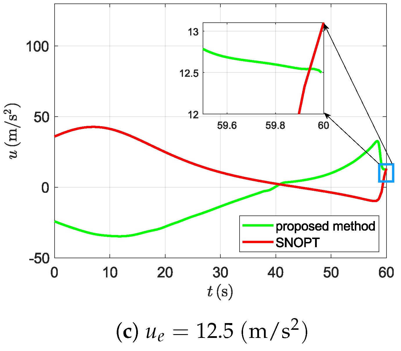
Figure 5.
Trajectories generated by Monte Carlo test
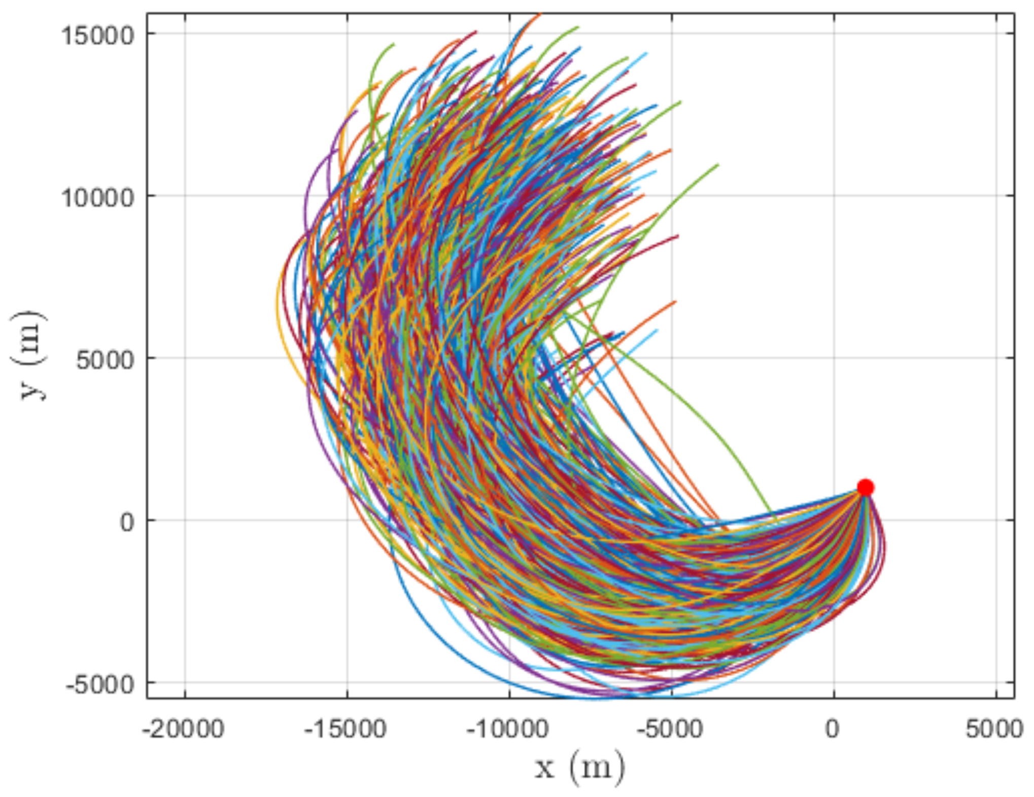
Figure 6.
Histograms for errors of Monte Carlo test.
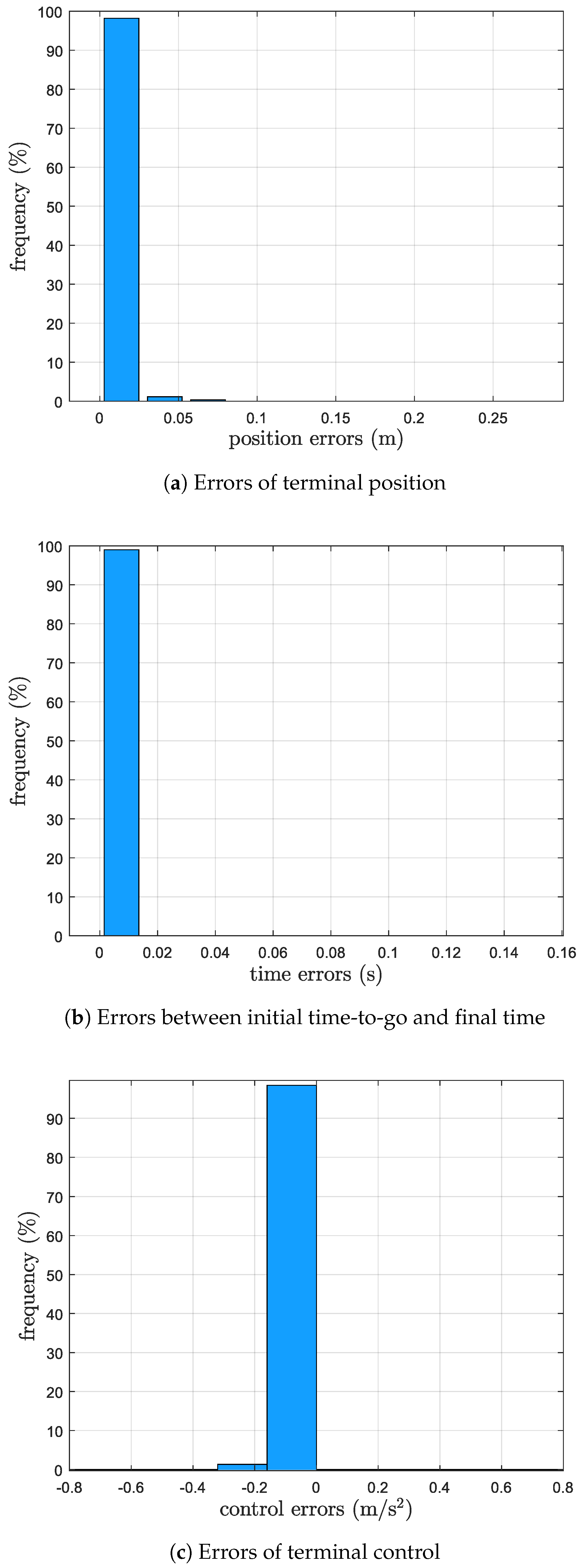

Table 1.
The initial conditions of the three UAVs.
| Initial Conditions | V | |||
|---|---|---|---|---|
Table 2.
The control effort for three UAVs.
Disclaimer/Publisher’s Note: The statements, opinions and data contained in all publications are solely those of the individual author(s) and contributor(s) and not of MDPI and/or the editor(s). MDPI and/or the editor(s) disclaim responsibility for any injury to people or property resulting from any ideas, methods, instructions or products referred to in the content. |
© 2025 by the authors. Licensee MDPI, Basel, Switzerland. This article is an open access article distributed under the terms and conditions of the Creative Commons Attribution (CC BY) license (http://creativecommons.org/licenses/by/4.0/).
Copyright: This open access article is published under a Creative Commons CC BY 4.0 license, which permit the free download, distribution, and reuse, provided that the author and preprint are cited in any reuse.


