Submitted:
15 April 2025
Posted:
15 April 2025
You are already at the latest version
Abstract
Accurate wind speed prediction is crucial for managing wind power generation systems. However, the stochastic nature of wind complicates the estimation of optimal intervals. This work analyzes the performance of hybrid machine learning techniques for modeling wind speed. Two deep learning models, Large Language Memory Long Short-Term Memory and Large Language Memory Convolutional, are proposed, along with two hybrid models from the literature, Bidirectional LSTM and Convolutional LSTM, for four-season forecasting in the Bodele low-pressure area. Meteorological data come from the NASA Power/Dav site. Data processing includes removal of outliers and imputation of missing values by mean, median, or predictive models, performed with Python. The four hybrid models use the Adam algorithm to optimize predictions. The predicted values calculate wind turbine power, efficiency, and storage energy. Results show that performance indicators vary: MAE from 0.020 to 0.586, RMSE from 0.027 to 0.848, and R² from 0.902 to 0.966. Energy predictions for a 5 MW wind turbine range from 4.91 MWh in winter to 0.89 MWh in summer. The CL-LSTM and LLM-LSTM models give high wind speeds in summer and winter, providing insights for developing efficient models for similar applications, both for researchers and companies.
Keywords:
analysis
; alorithme adam
; machine learning
; prediction
; modeling
; bodele of triangle
1. Introduction
In recent years, with fossil fuels in short supply and environmental problems on the increase, the scale of clean energy production has expanded rapidly [1]. Wind power generation has become one of the most important renewable energy production methods due to its clean, economic and sustainable advantages [2]. By the end of 2019, total wind power capacity worldwide stood at over 651 GW, of which 60.4 GW of wind power capacity had been installed worldwide [3]. Although wind power generation technology is becoming increasingly mature, the stability, security, and economics of wind power and the electricity grid are affected by its intermittency, randomness, and the uncertainty of wind power generation [4]. At the same time, the uncertainty of wind power generation will also have impacts on electricity market design, wind system planning and deployment, power grid dispatch, transmission capacity upgrades and other issues [5]. Therefore, accurate and efficient wind energy forecasting technology is indispensable and of great importance for safe, stable and economical operation.
Currently, many researchers around the world have conducted extensive research into wind energy forecasting methods. According to different forecasting principles, wind energy forecasting methods can be summarized into three main categories: the physical model, the statistical model and the machine learning model [6,7]. Of these methods, the physical model relies on meteorological and wind speed information from numerical weather prediction, which requires big data modeling. This method is suitable for large-scale, long-term forecasts and is not applicable to small areas and short-term forecasts [8]. Statistical methods produce forecasts based on the spatial and temporal analysis of search data, including the Kalman filter [9], regression methods [10,11], exponential smoothing methods [12] and time series analysis methods [13]. Although statistical models perform well in simple time-series forecasting and short-term forecasting, they are inadequate in handling non-linear data and can accumulate errors in long-term forecasting [14]. In general, statistical methods outperform physical models in short-term wind energy forecasting [15].
1.1. Motivations
LLM-LSTM, BiLSTM, LLM-CNN and CL-LSTM methods for wind speed prediction applied to wind energy management systems are crucial for optimizing energy production. These models are capable of capturing long-term dependencies, improving forecast reliability by handling non-linear relationships, taking into account multiple variables and processing large datasets.
1.2. Literature Review
Wind speed prediction is an important field for renewable energy and meteorology. Hybrid deep learning models have been used to improve the accuracy of wind speed prediction. Table 1 presents a literature review of the different models used to predict wind speed.
Table 1 shows the results of the literature review. In 2020, Zhen, H., et al, [16] used the BiLSTM-CNN model, which performed well, with very low MAE and RMSE values, indicating high forecast accuracy. The very high coefficient of determination (R²) suggests that the model explains almost all variations in wind speed data. The joint use of BiLSTM to capture temporal characteristics and CNN for spatial characteristics was decisive for these results. Although the CL-LSTM model performed slightly less well than BiLSTM-CNN, it remained competitive, with a high R². MAE and RMSE values indicate good predictive capability, but performance could be improved by optimizing model parameters or integrating additional data. This model is particularly useful for applications where computational complexity needs to be reduced [17]. The CNN-LSTM also performed well, with a high R², indicating good forecast adequacy. However, it performs slightly less well than BiLSTM-CNN in terms of MAE and RMSE. The CNN-LSTM approach is effective in capturing temporal and spatial relationships, but perhaps less robust than the BiLSTM-CNN model in complex scenarios [18]. In 2023, Khan et al [19] used the BiLSTM model to demonstrate its effectiveness in wind speed prediction through several studies. The results show that BiLSTM, particularly when combined with other techniques such as CNN or feature engineering, can achieve very high levels of accuracy (R² > 0.995). In 2023, Khan et al [19] used the BiLSTM model for wind speed prediction, their result showing excellent performance with an R2 that explains 99.60% of the data variance. Although MAE and RMSE are relatively higher than those of other models, BiLSTM’s ability to capture temporal relationships makes it a robust choice for prediction. In 2022 Han et al [20] also used the hybrid CNN-BiLSTM model, offering very low prediction errors in MAE and RMSE. Although the R2 is slightly lower than that of BiLSTM, it still performs very well, indicating that this model is effective in capturing complex features in wind data. In 2024, Singh et al, [21] used the Bi-GRU model has very low errors, making it extremely accurate. Although its R2 is somewhat lower than that of BiLSTM, its ability to reduce the prediction error is remarkable, indicating that it is also very effective for the forecasting task. In 2020, Liu et al, [22] shows less impressive performance compared to the others, with a relatively low R2. This means that it explains only 81.70% of the data variance, and prediction errors are higher, suggesting that other models may be more appropriate. In 2023, Zhang et al [23] combines CNNs and LSTMs, and performs less well than the other models. With an R2 of 70.30%, it is less able to explain the variance in the data, suggesting that it could be improved or optimized for better performance.
1.3. Contribution
The main contributions in this study are:
- -
- Development of two hybrid deep learning models (LLM-LSTM and LLM-CNN) that integrate the LLM and LSTM methods, and CNN using the Adam optimization algorithm;
- -
- Comparison of proposed LLM-LSTM and LLM-CNN models with the hybrid methods already in the literature review, namely BiLSTM and CL-LSTM;
- -
- Determination of wind direction during different seasons of the year;
2. Material and Methods
2.1. Materials
2.1.1. Presentation of Study Sites
The Bodele depression is located in Chad’s Djourab desert, in the triangle formed by the Angamma, Tibesti and Ennedi massifs. The Bodele depression is the deepest part of the ancient Paleo-Chadian Sea and the country’s lowest point above sea level, home to around 40,000 inhabitants [24]. This region, with a surface area of 35,000 km2 and is known as the dustiest area on the planet [25]. Additionally, it is considered to be the world’s largest source of minerals [26]. This dust emission represents around 20% of global emissions, and these particles can reach the Amazon basin in ten days, contributing to the fertilization of this region. Historically, the depression was the bottom of a lake, the mega-lake Chad, which shrank as it dried up due to climatic conditions. The Bodele Low Level Jet, an air current specific to this region, favors the emission of dust. Although this phenomenon is unique to this region, the installation of wind turbines in the Bodele triangle could offer energy and environmental benefits, but it also poses logistical, environmental and social challenges. The Bodele depression is a unique location, both because of its role as a source of dust and its potential for wind energy, requiring a balanced approach to maximize benefits while minimizing negative impacts [27]. The geographical coordinates of the Bodele depression are 17° N and 18° E. Figure 1 shows the location of this area on the map.
2.1.2. Processing of Variables Used
The forecasting methods, including those used in this study, come from the NASA POWER website [28], a NASA-funded project aimed at improving understanding of the world’s energy resources. The processing of input variables for wind speed forecasting is a crucial step aimed at preparing the data so that they are suitable for the prediction models. After data collection, processing involves removing outliers, imputing by mean, median, and using predictive models to estimate missing values. In general, the aim of processing registration errors, outliers and missing values is to guarantee the quality and reliability of the data before it is used in analyses or predictive models. This helps to improve the accuracy of results and to make informed decisions based on reliable data.
This box plot shows the distribution of each variable after the extraction, transformation and loading process used in this study. These boxes illustrate the distribution and implementation of data quality improvements, such as handling missing values, detecting outliers and applying logarithmic transformations. This graphical representation serves to highlight the effectiveness of data pre-processing techniques in improving the distribution and quality of variables, which is a crucial step in guaranteeing the robustness and reliability of our subsequent machine learning models.
2.2. Methods
2.2.1. Determination of Input Variables and Normalizations
This subsection aims to determine which input variables are most correlated with the output variable. The correlation coefficient is calculated using formula (1) [29].
By calculating the correlation coefficient, we can identify the different variables that influence wind speed. It is important to note that a correlation coefficient close to 1 indicates better forecasting ability. This indicator varies between -1 and 1: a value of 1 means perfect agreement between the measured value and the output variable, while a value of -1 indicates perfect disagreement. A value of 0 suggests that there is no influence of the input variable on the output variable. Analysis of the correlations between the input variables and the output variable reveals relationships between them. To ensure accurate estimation and verification of prediction methods, data are divided into three sets. In the context of predictive models based on deep learning, the first step in data preparation is to check the stationarity of the data, which is carried out using the Dickey-Fuller (DF) test. The results indicate that the null hypothesis is accepted, meaning that the input variables are considered stationary. The second step consists of a correlation analysis to identify the relevant input variables. The autocorrelation function (ACF) is used to determine the inputs to the wind speed prediction model, identifying those with high correlation. As shown in Table 2, the time series data from all the study sites reveal a strongly elevated ACF. Considering x as the time series variable, this vector is then used to predict the y(i+1) value in the next step. Before integrating the data into the network, it is essential to normalize them. Equations (2) and (3) present the normalization formulas [30].
Table 2 details the correlation coefficient between the various model input variables and wind speed. More specifically, it shows that wind direction and relative humidity display negative correlations with wind speed, meaning that an increase in either of these variables is associated with a decrease in wind speed. On the other hand, temperature and atmospheric pressure show positive correlations, indicating that an increase in these two parameters is associated with an increase in wind speed. These results suggest complex interactions between climate variables and wind dynamics, essential for a thorough understanding of weather patterns.
2.2.2. The Bidirectional Long Short-Term Memory (BiLSTM) Model
The BiLSTM model is a variant of the LSTM model, designed to capture temporal dependencies in time series, in both forward and reverse directions. This makes it a powerful model for tasks requiring the understanding of past and future relationships in data sequences. An LSTM is a type of recurrent neural network (RNN) that improves on the classic RNN by incorporating memory cells to store long-term information. LSTM is capable of better retaining relevant information while forgetting unnecessary information. This makes it effective for long-duration sequences where simple RNNs fail due to the gradient problem disappearing. Unlike a conventional LSTM, which processes sequences in a single direction from past to future, a BiLSTM processes sequences in both directions. From the first to the last data of the sequence. From the last to the first data item in the first sequence. Each LSTM cell therefore learns two distinct representations: one that takes into account past information and one that takes into account future information. This enables the model to understand both past and future context, which can be crucial in time-series prediction tasks where future and past values can influence the current prediction. A sequence of temporal data. For example, a series of sensor values at different times. Each sequence passes through two LSTM layers, one processing the data in the forward direction, the other in the reverse direction. The two outputs are then combined to form the final output. It is often a dense layer for generating the final prediction, which may be a single value in the case of regression, or several categories in the case of classification. The model takes into account past and future information, which can improve prediction accuracy. For tasks where the future context is as important as the past, BiLSTM better captures these dependencies. Bidirectional processing adds computational complexity, increasing the computation time and memory required. LSTM models, in particular BiLSTMs, often require a large amount of data to properly generalize and learn significant dependencies in sequences [31]. The architecture of a BiLSTM is illustrated in Figure 3.
To better understand BiLSTM, it is useful to start with the formulation of a classical LSTM, as described by equations (4) to (11) for a unidirectional LSTM.
Combining the two hidden forward and reverse states to form the output at each time step t.
2.2.3. Large Language Memory LSTM Model (LLM-LSTM)
The LLM-LSTM model is a hybrid prediction model proposed in this study. It combines the LLM model and the LSTM model. This combination combines the strengths of each component to provide a better prediction. The LLM model is based on a transform network architecture, which is designed for text processing tasks, but is adapted here for time series prediction. The role of LLM is to capture long-term trends in the input data, based on its ability to process long sequences. It extracts global characteristics from data over long periods thanks to its attention mechanisms. The LSTM model is a type of recurrent neural network designed to process time series. This model is given by equation (12).
The proposed model improves predictive accuracy by capturing trends, temporal dependencies and the flexibility to integrate additional data. Its architecture is shown in Figure 2.
In Figure 4, the input data are time series. On the embedding layer (LLM), the input data are passed through the embedding layer to obtain vector representations of size (d). Each element of the input vector is associated with an embedding vector. The vector representations obtained from the embedding layer are passed through the LSTM layer. The LSTM layer consists of L layers, each with h units. Each vector unit of the previous layer and produced an output of size (h) the output of the LSTM layer are merged with the vector representations of the embedding layer (LLM). Merging can be performed using operations such as concatenation or addition. The output of the fusion layer is passed through the prediction layer to obtain the final prediction.
2.2.4. The Convolutional Neural Networks and Long Short-Term Memory (CL-LSTM) Model
The hybrid CL-LSTM model is a combination of two neural network architectures. The formula is presented by equation (13) [32,33]. Figure 5 shows the architecture of the model.
Figure 5 shows the convolutional neural network and the recurrent neural network LSTM. The CNN layers capture the spatial structures of the data, while long-term temporal dependencies are captured by the LSTM network. In the hybrid CL-LSTM model, convolutional layers are used upstream to extract relevant spatial features from the input data, while LSTM layers are used to process temporal sequences and capture long-term dependencies in the data.
2.2.5. The Large Language Memory Convolutional Network (LLM-CNN) Model
The LLM-CNN model is a deep learning architecture that combines the advantages of convolutional neural networks and memory mechanisms to process sequences of data, particularly in the field of natural language processing and other applications requiring efficient management of contextual information. The convolution layer uses convolutional layers to extract local features from input data. This enables the capture of patterns and relationships in data, whether text, images or other types of structured data. Memory integrates memory mechanisms to manage long-term dependencies. This enables the model to remember relevant information over long sequences, which is crucial for tasks such as machine translation or text generation. The combination of CNN and memory mechanisms benefits from the strengths of both approaches, improving the model’s ability to process sequences while maintaining computational efficiency. Equations (14) to (22) present the different stages of the model.
LLM layer formula
Memory update:
Convolution layer formula
Pooling formula:
Output layer formula
The input to our model is the time series. The CNN layer extracts features and patterns in the data, and the LLM layer captures long-term dependencies and contextual relationships in the sequences. But beforehand, the data are normalized to improve model convergence. Then divided into windows to create input samples. The time series data are organized into windows, where each window represents a segment of the time series. The two layers are then concatenated to create an enriched feature vector. Pass this vector through fully connected layers to make predictions.
The following diagram shows the process from data collection to wind speed prediction.
Figure 7 provides a detailed illustration of the various steps involved, from data collection to wind speed prediction. This process includes the initial collection of meteorological data, its processing and analysis, as well as the statistical or modeling methods and optimization algorithm used to make the forecast. Each step is crucial in ensuring the accuracy of the final results and the reliability of the predictions.
2.2.6. Advantages and Disadvantages of the Different Models
Table 3 summarizes the advantages and disadvantages of different deep learning models for solar radiation prediction.
2.2.7. Model Performance Evaluation
To evaluate the performance of four hybrid machine learning models, hold-out and k-fold cross-validation techniques were applied. These methods provide a reliable estimate of model performance using different data partitions. The results of these evaluations are summarized in Table 3, providing an overview of the comparative performance of the models analyzed.
2.2.8. Wind Speed Modeling
2.2.8.1. Weibull Parameters
The Weibull distribution is a continuous probability distribution used to model reliability-related phenomena. The Weibull distribution is defined by two main parameters: Scale parameter (λ): this parameter determines the scale of the distribution. It is related to the median value of the distribution. Shape parameter (k): this parameter determines the shape of the distribution. It plays an important role in modeling failure rates. Variations in wind speed are characterized by the distribution of two functions: the probability density function and the distribution function. The probability density function is given by equation (26) [38].
The Weibull distribution function f(v) gives the probability that the wind speed is less than or equal to v in equation (27) [39].
The mean wind speed according to the Weibull distribution is given by formula (28).
The Weibull distribution is very important for describing the statistical properties of wind speed. There are several methods for determining the parameters k and c from site wind data. The most common are: the graphical method, the moment method, the maximum likelihood method, the modified maximum likelihood method and the standard deviation method. The wind variability method is defined by equation (29) [39,40].
The factor c is given by equation (30)
is a function that characterizes the shape of the frequency distribution and the asymmetry of the velocity frequency distribution, and is given by relations (31) and (32).
2.2.8.2. Extrapolation of Wind Speed as a Function of Height
In order to obtain adequate speeds for the operation of Gamesa G128-5.0MW wind turbines, extrapolations are made to increase the wind speed at 100 m height. Since wind speed measurements are taken at 10 m above ground level, the characteristics given in the data sheet for our wind turbine, presented in Table 7, indicate that it is necessary to install the turbine at a well-defined height. Equations (33-34) are used to calculate this speed [41].
2.2.8.3. Extrapolation of Weibull Parameters as a Function of Height
2.2.8.4. Power Density of a Wind Turbine
Equation (38) can be used to estimate the recoverable power at a site [39].
WED (Wind Energy Density) quantifies the energy produced over a time T. The time T depends on the availability factor and the load factor. This is expressed by equation (39).
2.2.8.5. Wind Turbine Power Calculation
Obtaining power in W from the values obtained when predicting wind speed using Weibull parameters is done by equation (40 or 41) [44].
The production of a given amount of energy by a wind turbine depends on the complex choice of suitable turbines, and it is essential to calculate the load factor to correct this problem, using formula (42).
2.2.8.6. Balancing Production with Demand
2.2.8.7. Management of High and Low Production Periods
To manage periods of high production, it may be necessary to implement energy storage systems, such as batteries [47].
During surplus production, energy can be stored. When production is low, stored energy can be used to meet demand.
In Figure 8, wind turbines convert the kinetic energy of the wind into electrical energy. This stage involves turbines that capture the wind and generate electricity. The electricity generated can be used immediately to power homes and businesses, or fed into the electricity grid. It can also be used to power specific systems such as pumps or electrical appliances. When electricity production exceeds demand, excess energy can be stored. This is usually done using batteries or other storage technologies, enabling later use when production is low or demand is high.
2.2.8.8. Wind Turbine Reliability Analysis
A wind turbine’s load factor is an indicator of its efficiency and performance in converting wind energy into electricity. Expressed as a percentage, it compares the energy actually produced by the turbine with its theoretical maximum capacity. To calculate the load factor (LF), five parameters are taken into account: two are site-dependent (form factor k and scale factor c), while three are supplied by the turbine manufacturer (starting speed VD, nominal speed VN and stopping speed VA) [48].
When the load factor exceeds 25%, it can be concluded that this site can generate electrical energy using wind speed [49].

Table 5.
Characteristics of the Gamesa G128-5.0MW wind turbine.
| Manufacturer | Gamesa |
|---|---|
| Rated power | 5 MW |
| Starting speed | 4 m/s |
| Nominal wind speed | 14.0 m/s |
| Disconnection speed | 27. 0 m/s |
| Hub height | 81 à 120 m |
| Rotor diameter | 128.0 m |
| Area swept by blades | 7 854 m² |
3. Validation of Results with Similar Hybrid Models
Numerous studies have explored the use of recurrent neural network models for wind speed forecasting, due to their ability to capture complex temporal dependencies.
Case 1: In 2024 Li et al [50] investigated a spatio-temporal graph neural network based on attention and short- and long-term memory (ASTGNN-LSTM) for wind speed prediction, obtaining an MAE of 0.757, an RMSE of 1.003 m/s and an R² of 0.261. In our study, the LLM-CNN model produced an RMSE of 0.752 m/s and an R² of 0.943, demonstrating competitive performance against literature results.
Case 2: In 2022, Johnson et al, explored the use of BiLSTM models for wind speed prediction in a variety of climatic conditions. Their research revealed an RMSE of 0.600 m/s in summer and an R2 of 0.940, reinforcing the idea that LSTM-based models are particularly suited to capturing temporal variations in wind data. This study is in line with the second proposed model, LLM-LSTM, which displayed an RMSE of 0.629 m/s in summer and an R² of 0.933, confirming trends observed in other research, where LSTM models and their variants are often found to perform best for wind speed forecasting.
Case 3: In 2021, Lawal et al [51] used a CNN-BiLSTM model to predict wind speed. They obtained the best results, with minimum values of MAE = 0.298, RMSE = 0.428 m/s. In comparison, the results obtained with the BiLSTM model in our study obtained an RMSE of 0.745 m/s in spring and an R² of 0.944, which is in line with the performance observed in the literature.
Overall, the results of the study confirm the trends observed in the literature: LLM-LSTM and BiLSTM models perform best for wind speed forecasting, outperforming more conventional architectures. However, significant variations exist between seasons, indicating that specific adjustments to seasonal conditions could improve the performance of some models. These results underline the importance of model selection and hyperparameter optimization in maximizing the accuracy of wind speed forecasts.
4. Results and Discussion
The work carried out so far presents the steps taken to analyze the performance of hybrid automatic learning techniques of four models for wind speed prediction and modeling. The same data set is used to predict wind speed for the four seasons. The results obtained were analyzed using the statistical evaluation indicators described in section 2 and led to the following findings.
4.1. Presentation of Forecast Curves for Different Seasons
The wind speed forecast curves generated by the various hybrid deep learning algorithms for spring, winter, autumn and summer are presented in the following paragraph.
Figure 9 shows the predicted curves in comparison with actual test data for all four seasons, obtained from the LLM-LSTM, BiLSTM, LLM-CNN and CL-LSTM models. It is notable that the outputs of the different models follow very closely the same trend as the real data, with minimal deviation between the curves. This indicates an excellent ability of the models to adjust to variations in real data. In other words, these results testify to the robustness of the models, which were able to predict accurately without exaggerating or underestimating the values observed in the test data. This performance suggests that the models are well suited to forecasting wind generation, offering appreciable reliability for practical applications.
4.2. Presentation of Performance Statistics Values
This section examines the performance results obtained on the basis of the machine learning models developed in the previous areas.
Table 6 shows how the performance of each model varies with the different seasons. This allows us to observe how specific climatic conditions influence the results, offering an in-depth understanding of model behavior in varied seasonal contexts.
The LLM-LSTM model’s MAE (mean absolute error) results for the four seasons are shown in Table 6. In spring, the MAE is 0.556, indicating a moderate error and suggesting that predictions are fairly close to actual values. In summer, the MAE improves to 0.442, reflecting better model performance, indicating increased accuracy in wind speed prediction during this season. In autumn, the MAE reaches 0.435, representing the lowest error, underlining excellent forecast accuracy. In winter, the MAE is 0.469, slightly less accurate than in autumn, but the model still performs well. With regard to RMSE (root mean square error), which penalizes larger errors and is therefore sensitive to outliers, the results are as follows: in spring, RMSE is 0.820, indicating greater variability in predictions, suggesting that some forecasts may be less reliable. In summer, the RMSE improves to 0.629, showing greater consistency in forecasts. In autumn, the RMSE is 0.647, slightly lower than in summer, but still within an acceptable range. Finally, in winter, the RMSE increases to 0.689, which could indicate more variable wind conditions. The coefficient of determination (R²), which measures the proportion of data variance explained by the model, shows the following results: in spring, R² is 0.932, meaning that 93.2% of variance is explained by the model, an excellent result. In summer, R² is 0.933, indicating a stable performance close to that of spring. In autumn, this metric rises to 0.939, showing a slight improvement and increased model efficiency for this season. In winter, R² reaches 0.940, representing the best performance, with 94% of variance explained, indicating a very strong fit. The LLM-LSTM model demonstrates robust performance in predicting wind speed across seasons. The errors (MAE and RMSE) remain relatively low, while the coefficient of determination (R²) is high, indicating that the model is able to effectively capture variations in wind speed.
BiLSTM model: In spring, the MAE is 0.502, indicating a relatively low error and suggesting that predictions are fairly close to actual values. In summer, the MAE improves further, reaching 0.494, representing the best performance of the four seasons. This indicates that the model is particularly effective during this period. In autumn, the MAE increases to 0.586, showing a reduced accuracy compared to the other seasons. Finally, in winter, the MAE is 0.535, indicating a lower error than in autumn, but higher than in spring and summer. As for the RMSE, it shows a value of 0.745 in spring, reflecting moderate variability in predictions, suggesting that some estimates may be less accurate. In summer, the RMSE decreases to 0.686, indicating an improvement and more consistent predictions. In autumn, the RMSE climbs to 0.812, the highest value, suggesting that the model encounters difficulties in predicting wind speed during this season, leading to greater errors. In winter, the RMSE shows a value of 0.740, indicating an intermediate performance, slightly better than in autumn, but less effective than in spring and summer. As for the coefficient of determination, it is 0.944 in spring, meaning that 94.4% of the variance is explained, indicating an excellent fit. In summer, the R² is 0.920, which remains very good at 92% of variance explained, showing the model’s effectiveness. In autumn, this performance statistic decreases slightly to 0.904, indicating a reduced performance compared to other seasons. In winter, the R² reaches 0.931, representing 93.1% of the variance explained, indicating a strong fit. Overall, the BiLSTM model demonstrates robust performance in wind speed prediction, with relatively low errors (MAE and RMSE) and a high coefficient of determination (R²), underlining its ability to effectively model wind speed variations across seasons.
LLM-CNN model: In spring, the MAE is 0.503, indicating a relatively low error and predictions close to actual values. In summer, the MAE reaches 0.500, representing the best performance among the seasons, suggesting that the model is particularly effective during this period. In autumn, the value is 0.523, slightly higher than in spring and summer, but still within an acceptable range. In winter, the MAE is 0.566, the highest error, indicating reduced prediction accuracy during this season. In spring, the RMSE is 0.752, reflecting moderate variability in predictions, meaning that some may be less accurate. In summer, the RMSE shows a value of 0.689, indicating an improvement on spring and more consistent predictions. LLM-CNN model: In spring, the MAE is 0.503, indicating a relatively low error and predictions close to actual values. In summer, the MAE reaches 0.500, representing the best performance among the seasons, suggesting that the model is particularly effective during this period. In autumn, the value is 0.523, slightly higher than in spring and summer, but still within an acceptable range. In winter, the MAE is 0.566, the highest error, indicating reduced prediction accuracy during this season. In spring, the RMSE is 0.752, reflecting moderate variability in predictions, meaning that some may be less accurate. In summer, the RMSE shows a value of 0.689, indicating an improvement on spring and more consistent predictions. In summer, this metric is 0.919, meaning that 91.9% of the variance is explained, and testifying to the model’s effectiveness. In autumn, the R² is 0.914, showing a slight drop compared with previous seasons, indicating reduced performance. In winter, R² remains stable at 0.914, although errors are higher. Overall, the LLM-CNN model demonstrates solid performance in wind speed prediction, with relatively low errors (MAE and RMSE) and a high coefficient of determination (R²).
CL-LSTM model: In spring, the MAE is 0.636, indicating a relatively high error and suggesting that predictions are less accurate during this season. In summer, the MAE improves to 0.530, indicating better model efficiency during this period. In autumn, the MAE is 0.628, similar to that of spring, indicating moderate performance. In winter, the value drops to 0.020, revealing extremely low error and high accuracy in wind speed predictions. The RMSE in spring is 0.848, showing significant variability in predictions, suggesting that some estimates may be less reliable. In summer, the RMSE decreases to 0.679, indicating greater consistency in predictions. In autumn, the RMSE rises to 0.811, suggesting that the model has difficulty predicting wind speed during this season. In winter, the RMSE reaches 0.027, the lowest value, indicating a remarkable performance, with minimal errors. As for the coefficient of determination (R²), in spring it is 0.927, meaning that the model explains 92.7% of the variance, which is excellent. In summer, the R² is 0.922, still very good with 92.2% of variance explained, underlining the model’s efficiency. In autumn, the R² drops slightly to 0.902, indicating a reduced performance compared to other seasons. In winter, the R² reaches 0.966, representing the best performance, with 96.6% of variance explained, demonstrating a very solid fit. The CL-LSTM model shows variable performance in wind speed prediction, with particularly poor results in spring and autumn, but notable effectiveness in winter, where errors (MAE and RMSE) are relatively low.
The CL-LSTM model performed best in winter, while the BiLSTM and LLM-CNN models proved more effective in spring and summer. All models, however, struggled in autumn, posting higher errors, indicating that specific seasonal factors could affect prediction accuracy.
The results of the MAE, RMSE and R² metrics for the different models LLL-LSTM, BiLSTM, LLM-CNN, CL-LSTM over the spring, summer, autumn and winter seasons can be interpreted as follows.
4.3. Linear Regression and Residuals Graph
The models were trained on the same data set for all four seasons. The results show that these models are able to accurately predict the test dataset, as illustrated in Figure 10. This figure shows linear regression plots for the different methods. By analyzing these plots, we found that the CL-LSTM method offers the best prediction performance, with an R² value of 0.966, followed by the LLM-LSTM models, which is much more stable over the different seasons, and the BiLSTM model.
Figure 11 shows the scatterplots of predicted values against the linear line, representing the errors between predictions and actual wind speed values. The scatterplots show a high concentration of predictions around the perfect line, i.e. actual and predicted values, with less dispersion. We can see that the scatterplots of predictions are very close to the actual values for the different models for the different seasons of the year.
For Figure 12, it shows the residuals of the actual and predicted values against the indices or predicted values for each model. Good model accuracies can be observed. This is because the point clouds are randomly dispersed around the identity line.
4.4. Descriptive Statistical Analysis of Wind Speed Values
The descriptive analysis of wind speed values obtained during forecasting using the different models (LLM-LSTM, BiLSTM, LLM-CNN, CL-LSTM) for the autumn, spring, winter and summer seasons is presented below. Values are expressed in meters per second (m/s) and include maximum values, quartiles (Q1, Q2, Q3) and minimum values.
The descriptive statistical analysis in Table 7 shows that during spring, maximum wind speeds are highest in almost all models, reaching up to 28.65 m/s for LLM-LSTM and 28.39 m/s for LLM-CNN. This indicates that spring is a favorable season for optimal wind turbine operation, probably due to storms and unstable weather systems. Maximum values remain high, with peaks around 27.67 m/s for BiLSTM, which also suggests frequent windy conditions during winter. In summer, maximum wind speeds are significantly lower, reaching 19.54 m/s for LLM-LSTM, which is typical of more stable summer weather conditions. Q1 values (25th percentile) are relatively low in summer, indicating that 25% of wind speeds are below 2.36 m/s. The LLM-LSTM summer model shows low wind activity. The median (Q2) varies seasonally, with higher values in winter and spring, indicating that wind speeds are generally higher in these seasons. The 75th percentile values (Q3) are also higher in winter and spring, indicating that stronger winds are more frequent in these seasons. Minimum values are very low, especially in summer, when they reach 0.09 m/s for LLM-LSTM. This underlines the stability of summer weather conditions, with periods of calm winds.
Table 7.
Descriptive statistical values for prediction.
| Models | Autumn | Spring | Winter | Summer | |||||
|---|---|---|---|---|---|---|---|---|---|
| V(10m/s) | V(100m/s) | V(10m/s) | V(100m/s) | V(10m/s) | V(100m/s) | V(10m/s) | V(100m/s) | ||
| LLM_LSTM | Max | 15.70 | 24.88 | 18.08 | 28.65 | 17.36 | 27.51 | 12.33 | 19.54 |
| Q3 | 12.11 | 19.19 | 12.48 | 19.78 | 13.23 | 20.97 | 8.48 | 13.44 | |
| Q2 | 8.53 | 13.01 | 8.52 | 13.50 | 9.10 | 14.42 | 4.64 | 7.35 | |
| Q1 | 4.46 | 7.07 | 3.74 | 5.93 | 4.75 | 7.53 | 2.36 | 3.74 | |
| Min | 0.40 | 063 | 0.59 | 0.94 | 0.87 | 1.38 | 0.09 | 0.14 | |
| BiLSTM | Max | 15.94 | 25.26 | 17.49 | 27.72 | 17.46 | 27.67 | 12.22 | 19.37 |
| Q3 | 12.16 | 19.27 | 11.99 | 19.00 | 13.13 | 20.81 | 8.54 | 13.53 | |
| Q2 | 8.33 | 13.20 | 8.15 | 12.92 | 8.80 | 13.95 | 4.87 | 7.72 | |
| Q1 | 4.53 | 7.18 | 3.48 | 5.52 | 7.75 | 7.53 | 2.70 | 4.28 | |
| Min | 0.67 | 1.06 | 0.46 | 0.73 | 0.70 | 1.11 | 0.53 | 0.84 | |
| LLM_CNN | Max | 15.29 | 24.23 | 17.91 | 28.39 | 18.87 | 29.91 | 12.27 | 19.45 |
| Q3 | 11.96 | 18.96 | 12.21 | 19.35 | 14.07 | 22.30 | 8.54 | 13.53 | |
| Q2 | 8.08 | 12.81 | 8.19 | 12.98 | 9.27 | 14.69 | 4.63 | 7.34 | |
| Q1 | 4.48 | 7.10 | 3.33 | 5.28 | 4.63 | 7.34 | 2.43 | 3.85 | |
| Min | 0.33 | 0.52 | 0.17 | 0.27 | 0.98 | 1.55 | 0.23 | 0.36 | |
| CL_LSTM | Max | 15.52 | 24.60 | 17.58 | 27.86 | 17.76 | 28.15 | 12.31 | 19.51 |
| Q3 | 11.88 | 18.83 | 11.97 | 18.97 | 13.36 | 21.17 | 8.56 | 13.57 | |
| Q2 | 8.09 | 12.82 | 8.50 | 13.47 | 8.95 | 14.18 | 5.96 | 9.45 | |
| Q1 | 4.38 | 6.94 | 3.96 | 6.28 | 4.65 | 7.37 | 2.79 | 4.42 | |
| Min | 0.52 | 0.82 | 1.55 | 2.46 | 0.36 | 0.57 | 0.77 | 1.22 | |
4.5. Energy Prediction from Selected Model
Table 8 shows the electrical output of the wind turbine at the site in different seasons. This energy is highest in winter, spring and autumn. It is low in summer. The balance of high energy production is 4.91MWh minimum and 0.89 MWh.
The reference wind speed (V0) is highest in winter (8.95 m/s) and autumn (8.42 m/s), indicating that these seasons are conducive to stronger winds. In summer, on the other hand, the reference wind speed is significantly lower (5.025 m/s), which is typical of the calmer weather conditions of this season. K0 values are highest in winter (3.14) and autumn (3.05), indicating that wind speeds are more predictable and less dispersed during these seasons. In summer, the K0 value is lower (2.38), suggesting greater variability in wind speeds, consistent with more unstable weather conditions. Higher C0 values in winter (10.00 m/s) and autumn (9.42 m/s) indicate that turbines can operate efficiently at higher wind speeds during these seasons. In summer, the cut-off speed is lower (6.76 m/s), which may mean that turbines are less stressed due to lower wind speeds. FC values are highest in winter (0.69) and autumn (0.68), suggesting that turbines operate more efficiently in these seasons. In summer, FC is lowest (0.55), consistent with low wind speed and reduced energy production. The highest power values are observed in winter (4.91 MW/m2) and spring (4.25 MW/m2), indicating higher wind energy production during these seasons. In summer, power levels are significantly lower (0.89 MW/m2), reflecting low wind speeds and reduced energy production. In general, autumn and winter are the most favorable seasons for wind power generation, while summer production is very low, requiring another alternative source to make up the energy shortfall during this period.
4.6. Determining Wind Direction
To optimize the orientation of the wind turbine so that it effectively captures the prevailing wind, it is essential to determine the wind speed direction. To this end, we use a wind rose diagram, which illustrates the distribution of wind directions over a given period. This diagram was generated using WRPLOT software, a tool renowned for its efficiency in analyzing wind data. Figure 10 shows the corresponding diagrams for the different seasons of the year, highlighting seasonal variations in wind directions. This not only helps to identify the periods when the wind is strongest, but also to understand how wind direction changes over the seasons, which is crucial for maximizing wind energy production.
Interpretation of the wind roses for the different seasons, i.e. autumn, winter, spring and summer in the Bodele depression zone, is essential for assessing the wind potential of this region at various times of the year. As shown in Figure 10, during autumn, winter and spring, the dominant wind direction is north-northeast, with maximum frequencies of 55%, 54.5% and 30.4% respectively. In summer, the main wind direction changes to north-east, with a maximum frequency of 26.7%. The absence of calm winds in autumn is particularly promising for the development of wind energy, as it indicates a consistency in wind conditions, which is ideal for the installation of wind turbines. On the other hand, we observe a certain presence of calm winds in winter and spring, with frequencies of 0.09% and 0.31%, respectively, as well as 0.84% in summer. Although these calm winds are significant, they do not call into question the wind potential of winter and spring, which remain favorable, even if slightly less optimal than autumn. The installation of wind turbines must take account of prevailing wind directions to maximize their efficiency. In autumn, winter and spring, the prevailing wind direction is north-northeast. To optimize the capture of this wind, wind turbines should be oriented towards the north-northeast. This will ensure that they are positioned to capture the wind when it blows in this direction. Analysis reveals that wind conditions during autumn, winter and spring are favorable for wind energy projects, thanks to their reliability and consistency. In summer, the prevalence of calm winds is an obstacle to the installation of wind turbines. Thus, we can conclude that wind energy potential is acceptable in autumn, winter and spring, while it is less favorable in summer. These results underline the importance of a seasonal assessment to optimize the deployment of wind infrastructure in the region.
5. Conclusion and Outlook
This study evaluated the performance of four hybrid machine learning algorithms during different summers, springs, autumns, and winters in forecasting wind speed. The work takes into account various input data (temperature, relative humidity, velocity direction and solar radiation) from the NASA website. To evaluate the performance of machine learning algorithms, three metrics (RMSE, MAE, and R2) are examined in this research. Some important results can be drawn on the basis of current findings. In terms of R2, we can say that all the algorithms used gave good results. Indeed, algorithms in this research ranged from 0.902 in autumn to 0.966 in winter. For all the statistical measures for the seasons, the best results were obtained in winter. It can be seen that the majority of the values obtained are acceptable. This means that the majority of prediction results can be classified as reasonable or good predictions. However, by analyzing all the error magnitudes of the randomly determined observations in this research, it is deduced that the error magnitudes when using the CL-LSTM algorithms and the proposed LLM-LSTM model are very low compared to those of the other algorithms used. These results can help the Chadian government to make better decisions regarding the integration of wind energy as one of the main sources of electricity in the future. Future work will focus on the analysis of different wind speed profiles and the characteristics of data collected from meteorological stations. The aim will be to develop more effective prediction models. In addition, combined machine learning algorithms will be applied to improve forecast accuracy.
Funding
The study did not receive funding from any person or institution.
Data Availability Statement
The data that has been used is confidential.
Conflicts of Interest
The authors declare that there are no conflicts of interest with each other or with any person or institution.
Abbreviations and Acronyms
| WED | Wind Energy Density |
| V | Wind speed, m/s |
| Probability of observing wind seed | |
| Wind power, kwh | |
| VC | Cut-in wind speed, m/s |
| CF | Capacity Factor, % |
| N | The number of data pairs |
| X | The values of the first variable |
| Y | The values of the second variable |
| The sum of the values of the first variable | |
| The sum of the values of the first variable | |
| The sum of the values of the second variable | |
| The sum of the squares of the values of the first variable | |
| ∑Y2∑Y2 | The sum of the squares of the values of the second variable |
| Shape factor | |
| Scale factor (m/s) | |
| ,, | Heights |
| Reference speed | |
| Total number of trees in the ensemble | |
| Activation function | |
| Weight associated with each connection | |
| Specific regression model | |
| ƛ | Bias or intercept of the model |
| Predicted value | |
| Pegularization parameter | |
| Associated coefficient | |
| J(β) | Cost function to minimize |
| previous hidden state | |
| input at time t | |
| Sigmoid function. | |
| Element by element product (Hadamard product). | |
| Cell status at time t. | |
| ,,,,,,, | are the weights and biases learned by the network |
| Hidden state of front LSTM encoder. | |
| Hidden state of rear LSTM encoder | |
| is the word at time t ; | |
| is the embedding of the word x(t) | |
| is the hidden state of the LSTM layer at time | |
| is the output of the convolution layer | |
| is the output of the pooling layer at time t | |
| is the sigmoid activation function | |
| is the hyperbolic tangent activation function | |
| ,,,, | are the weight matrices |
| ,,,,, | are the bias vectors |
| ,,, | are the weight matrices for recurrent connections |
References
- Mehazzem, F., André, M., & Calif, R. (2022). Efficient output photovoltaic power prediction based on MPPT fuzzy logic technique and solar spatio-temporal forecasting approach in a tropical insular region. Energies, 15(22), 8671. [CrossRef]
- Afshar, K., Ghiasvand, F. S., & Bigdeli, N. (2018). Optimal bidding strategy of wind power producers in pay-as-bid power markets. Renewable Energy, 127, 575-586. [CrossRef]
- Shields, M., Stefek, J., Oteri, F., Kreider, M., Gill, E., Maniak, S., ... & Hines, E. (2023). A Supply Chain Road Map for Offshore Wind Energy in the United States (No. NREL/TP-5000-84710). National Renewable Energy Laboratory (NREL), Golden, CO (United States). [CrossRef]
- Naik, J., Bisoi, R., & Dash, P. K. (2018). Prediction interval forecasting of wind speed and wind power using modes decomposition based low rank multi-kernel ridge regression. Renewable energy, 129, 357-383. [CrossRef]
- uang, Y., Liu, S., & Yang, L. (2018). Wind speed forecasting method using EEMD and the combination forecasting method based on GPR and LSTM. Sustainability, 10(10), 3693. [CrossRef]
- Gangopadhyay, A., Seshadri, A. K., Sparks, N. J., & Toumi, R. (2022). The role of wind-solar hybrid plants in mitigating renewable energy-droughts. Renewable Energy, 194, 926-937. [CrossRef]
- Lahouar, A., & Slama, J. B. H. (2017). Hour-ahead wind power forecast based on random forests. Renewable energy, 109, 529-541. [CrossRef]
- Lee, J. A., Doubrawa, P., Xue, L., Newman, A. J., Draxl, C., & Scott, G. (2019). Wind resource assessment for Alaska’s offshore regions: validation of a 14-year high-resolution WRF data set. Energies, 12(14), 2780. [CrossRef]
- Zuluaga, C. D., Alvarez, M. A., & Giraldo, E. (2015). Short-term wind speed prediction based on robust Kalman filtering: An experimental comparison. Applied Energy, 156, 321-330. [CrossRef]
- Torres, J. L., Garcia, A., De Blas, M., & De Francisco, A. (2005). Forecast of hourly average wind speed with ARMA models in Navarre (Spain). Solar energy, 79(1), 65-77. [CrossRef]
- He, Q., Wang, J., & Lu, H. (2018). A hybrid system for short-term wind speed forecasting. Applied energy, 226, 756-771. [CrossRef]
- Cadenas, E., Jaramillo, O. A., & Rivera, W. (2010). Analysis and forecasting of wind velocity in chetumal, quintana roo, using the single exponential smoothing method. Renewable Energy, 35(5), 925-930. [CrossRef]
- Samet, H., & Marzbani, F. (2014). Quantizing the deterministic nonlinearity in wind speed time series. Renewable and Sustainable Energy Reviews, 39, 1143-1154. [CrossRef]
- Ouyang, T., Zha, X., & Qin, L. (2017). A combined multivariate model for wind power prediction. Energy Conversion and Management, 144, 361-373. [CrossRef]
- Lahouar, A., & Slama, J. B. H. (2017). Hour-ahead wind power forecast based on random forests. Renewable energy, 109, 529-541. [CrossRef]
- Zhen, H., Niu, D., Yu, M., Wang, K., Liang, Y., & Xu, X. (2020). A hybrid deep learning model and comparison for wind power forecasting considering temporal-spatial feature extraction. Sustainability, 12(22), 9490. [CrossRef]
- Liu, M., Cao, Z., Zhang, J., Wang, L., Huang, C., & Luo, X. (2020). Short-term wind speed forecasting based on the Jaya-SVM model. International Journal of Electrical Power & Energy Systems, 121, 106056. [CrossRef]
- Wang, J. Z., Wang, Y., & Jiang, P. (2015). The study and application of a novel hybrid forecasting model–A case study of wind speed forecasting in China. Applied Energy, 143, 472-488. [CrossRef]
- Khan, S. U., Khan, N., Ullah, F. U. M., Kim, M. J., Lee, M. Y., & Baik, S. W. (2023). Towards intelligent building energy management: AI-based framework for power consumption and generation forecasting. Energy and buildings, 279, 112705. [CrossRef]
- « Licht, A., Folch, A., Sylvestre, F., Yacoub, A. N., Cogné, N., Abderamane, M., ... & Deschamps, P. (2024). Provenance of aeolian sands from the southeastern Sahara from a detrital zircon perspective. Quaternary Science Reviews, 328, 108539. [CrossRef]
- Remini, B. (2018). Tibesti-Ennedi-Chad Lake: the triangle of dust impact on the fertilization of the Amazonian forest. LARHYSS Journal P-ISSN 1112-3680/E-ISSN 2521-9782, (34), 147-182.
- Washington, R., Todd, M. C., Engelstaedter, S., M’Bainayel, S., & Mitchell, F. (2006). Dust and the low level circulation ov er the Bodele Depression, Northern Chad. Journal of Geophysical Research, 111. [CrossRef]
- Remini, B. (2018). Tibesti-Ennedi-Chad Lake: the triangle of dust impact on the fertilization of the Amazonian forest. LARHYSS Journal P-ISSN 1112-3680/E-ISSN 2521-9782, (34), 147-182.
- Tatari, O., & Kucukvar, M. (2011). Cost premium prediction of certified green buildings: A neural network approach. Building and Environment, 46(5), 1081-1086. [CrossRef]
- Fogno Fotso, H. R., Aloyem Kazé, C. V., & Djuidje Kenmoé, G. (2021). A novel hybrid model based on weather variables relationships improving applied for wind speed forecasting. International Journal of Energy and Environmental Engineering, 1-14. [CrossRef]
- Wan, A., Peng, S., Khalil, A. B., Ji, Y., Ma, S., Yao, F., & Ao, L. (2024). A novel hybrid BWO-BiLSTM-ATT framework for accurate offshore wind power prediction. Ocean Engineering, 312, 119227. [CrossRef]
- Huang, C., Bu, S., Chen, W., Wang, H., & Zhang, Y. (2024). Deep Reinforcement Learning-Assisted Federated Learning for Robust Short-Term Load Forecasting in Electricity Wholesale Markets. IEEE Transactions on Network Science and Engineering. [CrossRef]
- Gollagi, S. G., & Balasubramaniam, S. (2023). Hybrid model with optimization tactics for software defect prediction. International Journal of Modeling, Simulation, and Scientific Computing, 14(02), 2350031. [CrossRef]
- Tefera, E., Martínez-Ballesteros, M., Troncoso, A., & Martínez-Álvarez, F. (2023, August). A new hybrid cnn-LSTM for wind power forecasting in ethiopia. In International Conference on Hybrid Artificial Intelligence Systems (pp. 207-218). Cham: Springer Nature Switzerland. [CrossRef]
- Niu, X., & Wang, J. (2019). A combined model based on data preprocessing strategy and multi-objective optimization algorithm for short-term wind speed forecasting. Applied Energy, 241, 519-539. [CrossRef]
- Nematchoua, M. K., Orosa, J. A., & Afaifia, M. (2022). Prediction of daily global solar radiation and air temperature using six machine learning algorithms; a case of 27 European countries. Ecological Informatics, 69, 101643. [CrossRef]
- Fan, J., Wang, X., Wu, L., Zhang, F., Bai, H., Lu, X., & Xiang, Y. (2018). New combined models for estimating daily global solar radiation based on sunshine duration in humid regions: a case study in South China. Energy conversion and management, 156, 618-625. [CrossRef]
- Satwika, N. A., Hantoro, R., Septyaningrum, E., & Mahmashani, A. W. (2019). Analysis of wind energy potential and wind energy development to evaluate performance of wind turbine installation in Bali, Indonesia. Journal of Mechanical Engineering and Sciences, 13(1), 4461-4476. [CrossRef]
- Cetinay, H., Kuipers, F. A., & Guven, A. N. (2017). Optimal siting and sizing of wind farms. Renewable Energy, 101, 51-58. [CrossRef]
- Boro, D., Donnou, H. E. V., Kossi, I., Bado, N., Kieno, F. P., & Bathiebo, J. (2019). Vertical profile of wind speed in the atmospheric boundary layer and assessment of wind resource on the Bobo Dioulasso site in Burkina Faso. [CrossRef]
- Soulouknga, M. H., Oyedepo, S. O., Doka, S. Y., & Kofane, T. C. (2020). Evaluation of the cost of producing wind-generated electricity in Chad. International Journal of Energy and Environmental Engineering, 11, 275-287. [CrossRef]
- Shakoor, R., Hassan, M. Y., Raheem, A., & Rasheed, N. (2016). Wind farm layout optimization using area dimensions and definite point selection techniques. Renewable energy, 88, 154-163. [CrossRef]
- Lazić, L., Pejanović, G., & Živković, M. (2010). Wind forecasts for wind power generation using the Eta model. Renewable Energy, 35(6), 1236-1243. [CrossRef]
- Nediguina, M. K., Abdraman, M. A., Barka, M., & Tahir, A. M. (2022). Electric Water Pumping Powered by a Wind Turbine in North East Chad. World Journal of Applied Physics, 7(2), 21-31. [CrossRef]
- El Khadimi, A., Bchir, L., & Zeroual, A. (2004). Dimensionnement et Optimisation Technico-économique d’un système d’Energie Hybride photovoltaïque-Eolien avec Système de stockage. Journal of Renewable Energies, 7(2), 73-83. [CrossRef]
- Pavarini, C., Battery storage is (almost) ready to play the flexibility game, IEA: International Energy Agency. France. Retrieved from https://coilink.org/20.500.12592/8sw59s.
- Amrouche, B., & Le Pivert, X. (2014). Artificial neural network based daily local forecasting for global solar radiation. Applied energy, 130, 333-341. [CrossRef]
- Foley, A. M., Leahy, P. G., Marvuglia, A., & McKeogh, E. J. (2012). Current methods and advances in forecasting of wind power generation. Renewable energy, 37(1), 1-8. [CrossRef]
- Bekele, G., & Tadesse, G. (2012). Feasibility study of small Hydro/PV/Wind hybrid system for off-grid rural electrification in Ethiopia. Applied Energy, 97, 5-15. [CrossRef]
- Lawal, A., Rehman, S., Alhems, L. M., & Alam, M. M. (2021). Wind speed prediction using hybrid 1D CNN and BLSTM network. IEEE Access, 9, 156672-156679. [CrossRef]
- Li, P., Yang, H., Wu, H., Wang, Y., Su, H., Zheng, T., ... & Han, Y. (2024). Deep learning model for solar and wind energy forecasting considering Northwest China as an example. Results in Engineering, 24, 102939. [CrossRef]
- Aguiar, L. M., Pereira, B., David, M., Díaz, F., & Lauret, P. (2015). Use of satellite data to improve solar radiation forecasting with Bayesian Artificial Neural Networks. Solar Energy, 122, 1309-1324. [CrossRef]
- Foley, A. M., Leahy, P. G., Marvuglia, A., & McKeogh, E. J. (2012). Current methods and advances in forecasting of wind power generation. Renewable energy, 37(1), 1-8. [CrossRef]
- Kidmo, D. K., Bogno, B., Deli, K., & Goron, D. (2020). Seasonal wind characteristics and prospects of wind energy conversion systems for water production in the far North Region of Cameroon. Smart Grid and Renewable Energy, 11(9), 127-164. [CrossRef]
- Li, P., Yang, H., Wu, H., Wang, Y., Su, H., Zheng, T., ... & Han, Y. (2024). Deep learning model for solar and wind energy forecasting considering Northwest China as an example. Results in Engineering, 24, 102939. [CrossRef]
- Lawal, A., Rehman, S., Alhems, L. M., & Alam, M. M. (2021). Wind speed prediction using hybrid 1D CNN and BLSTM network. IEEE Access, 9, 156672-156679. [CrossRef]
Figure 1.
View of the study site.
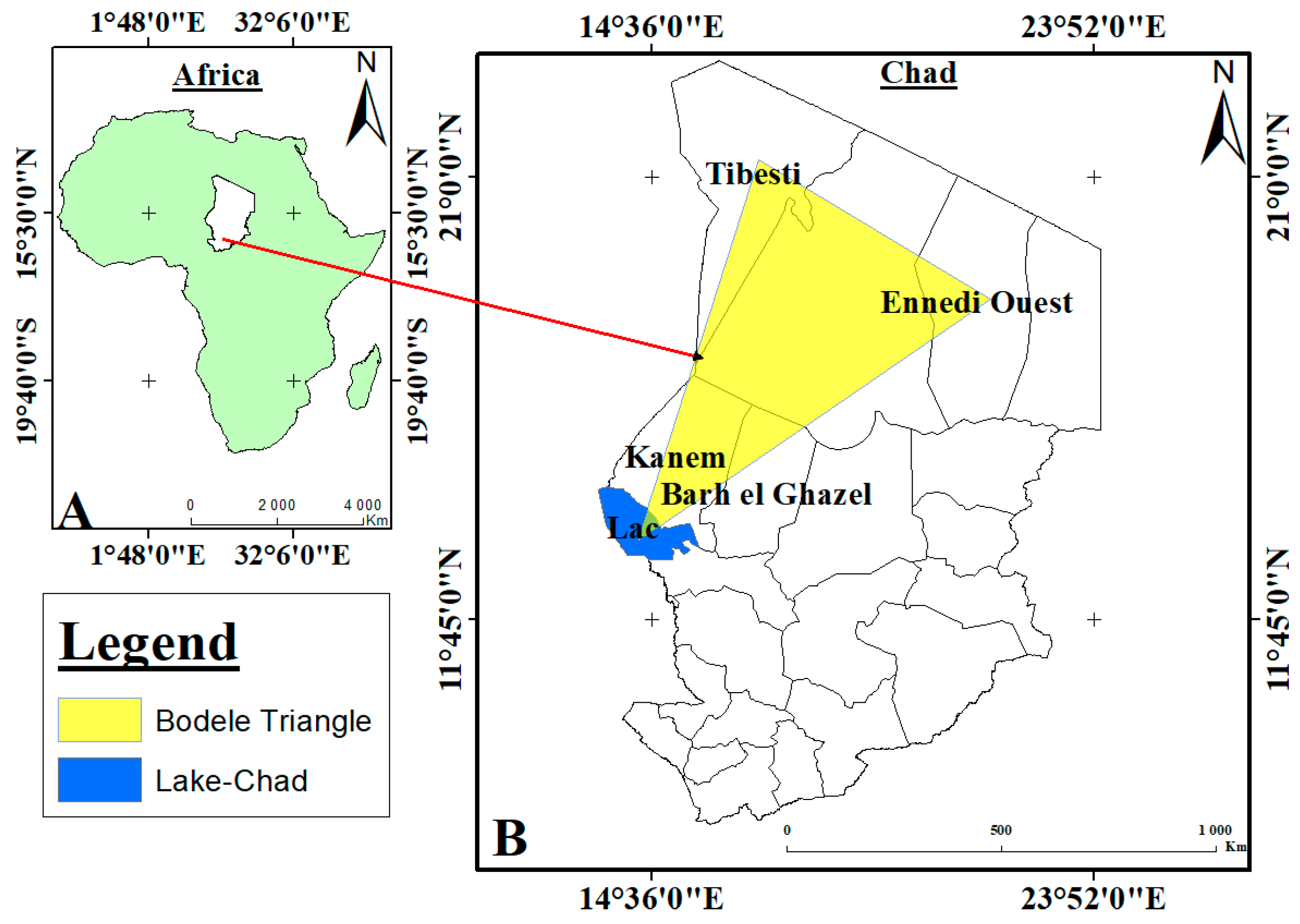
Figure 2.
Box-whisker plot of (a) untreated and (b) treated values.
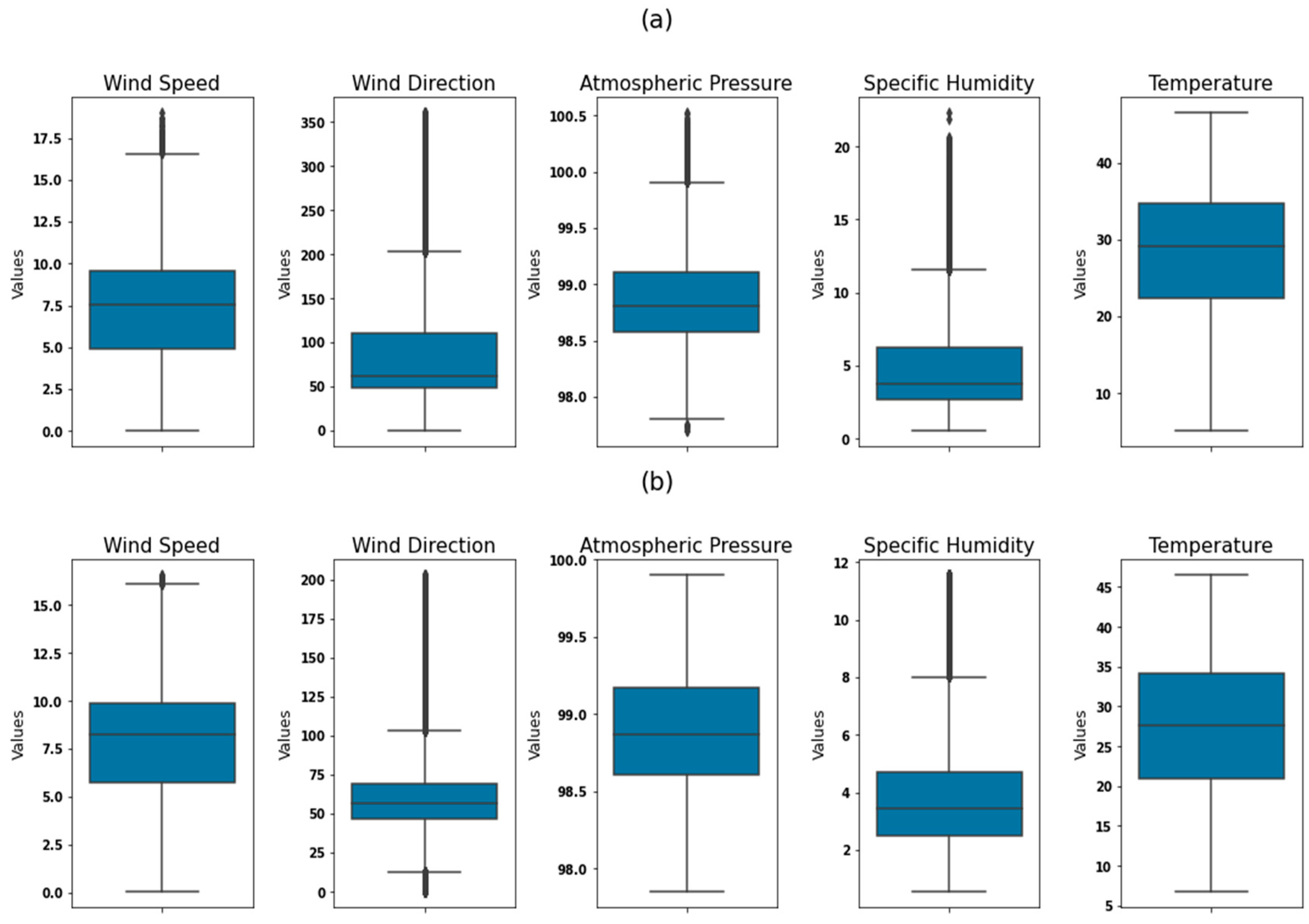
Figure 3.
Architecture of the BiLSTM model.
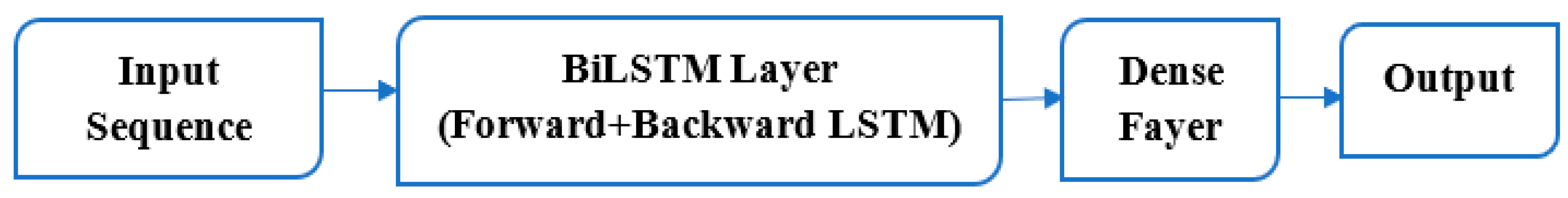
Figure 4.
LLM-LSTM model configuration presentation.
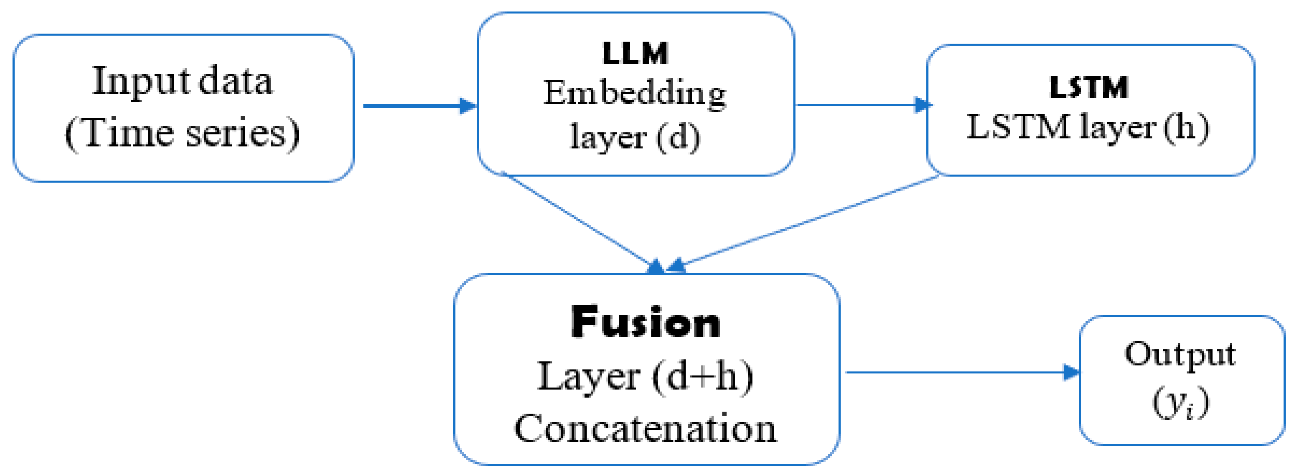
Figure 5.
Architecture of the CL-LSTM hybrid model [34].
Figure 5.
Architecture of the CL-LSTM hybrid model [34].
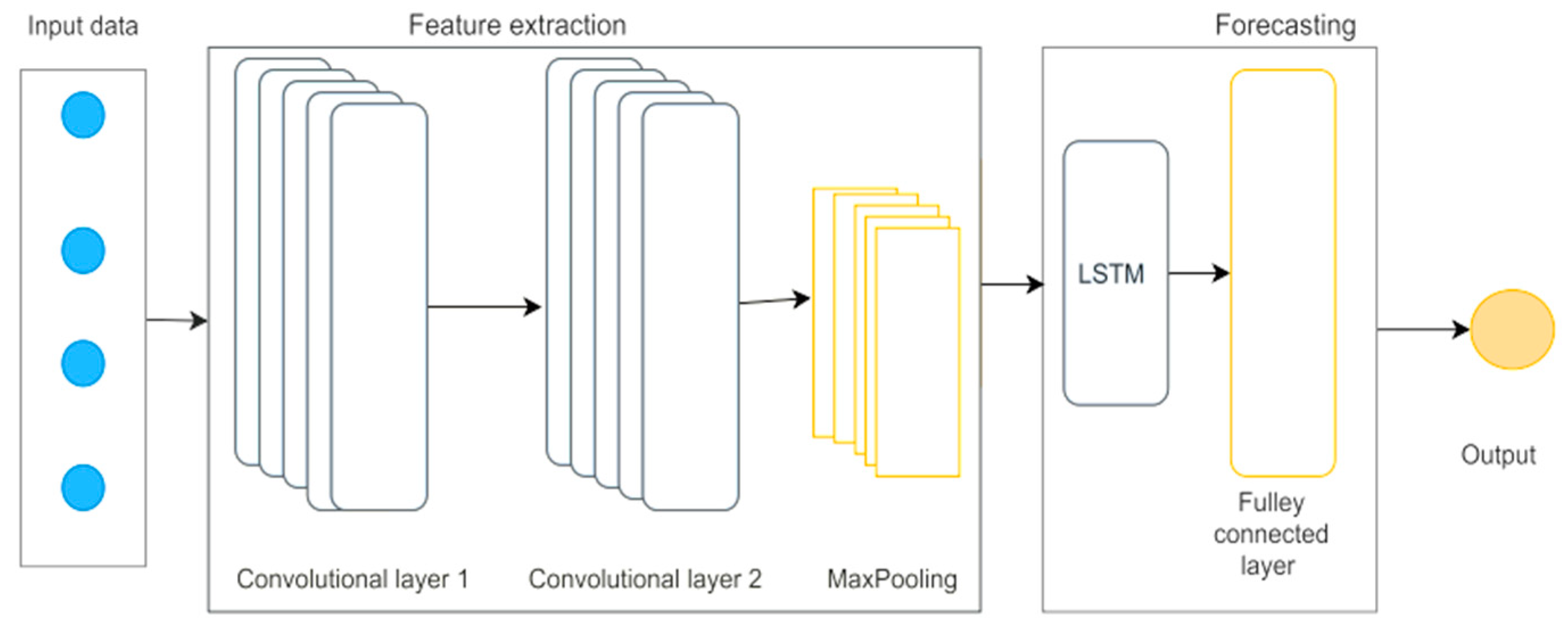
Figure 6.
Representation of LLM-CNN model architecture.
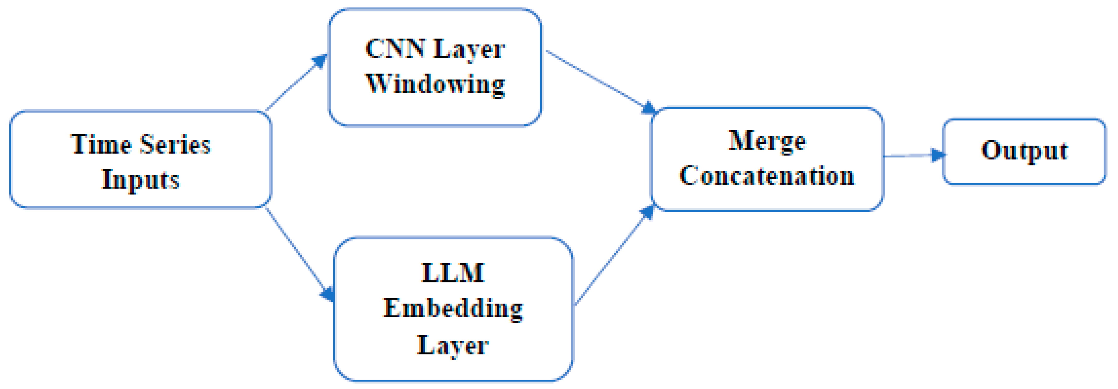
Figure 7.
Study diagram.
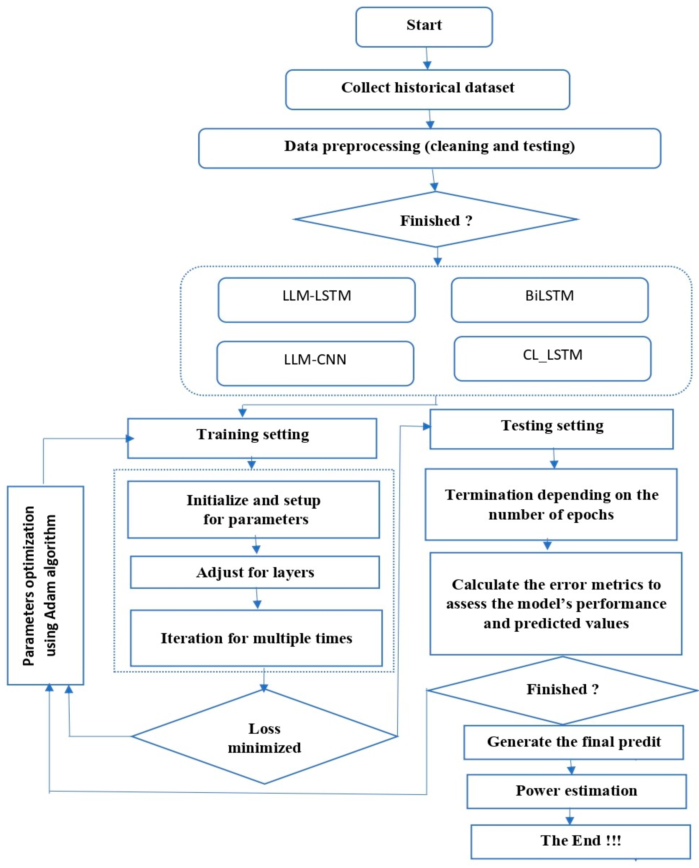
Figure 8.
Wind energy management system.
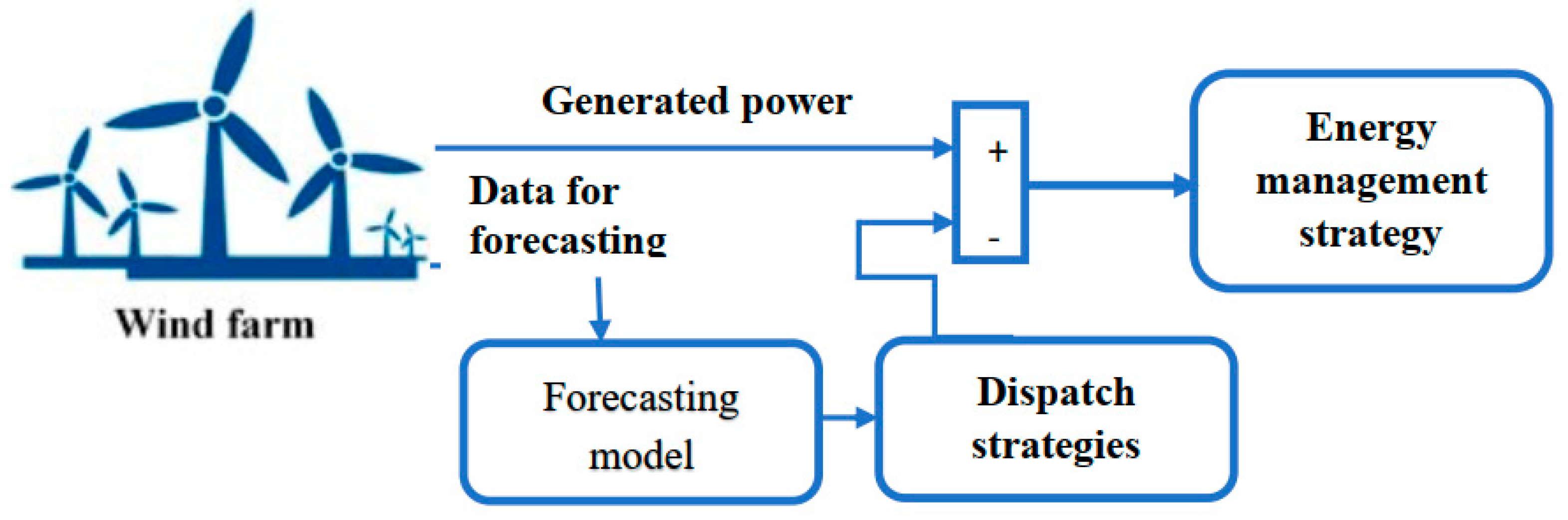
Figure 9.
Wind speed forecast curves for different seasons.
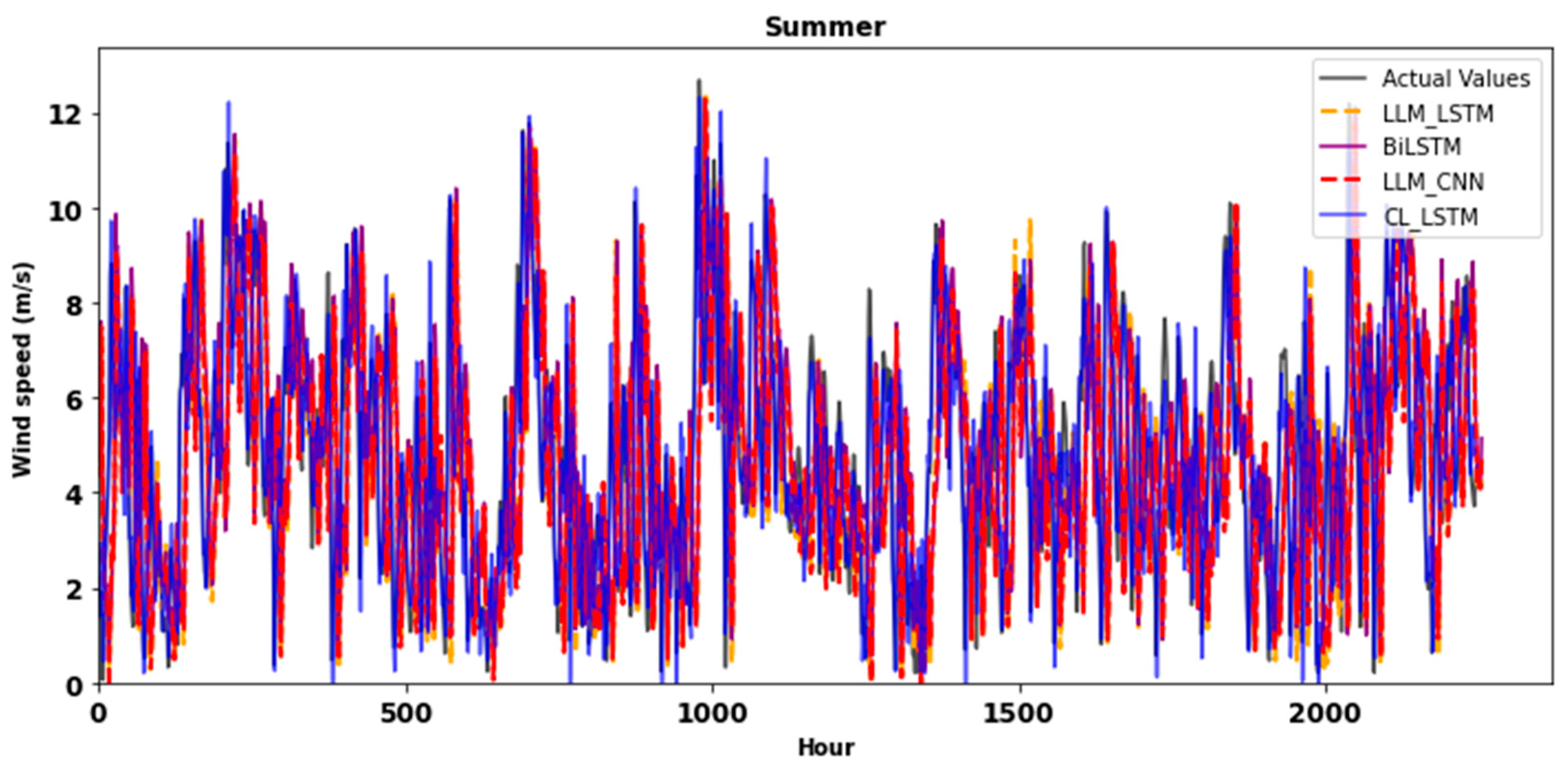

Figure 10.
Graphical representation of statistical coefficients of determination.

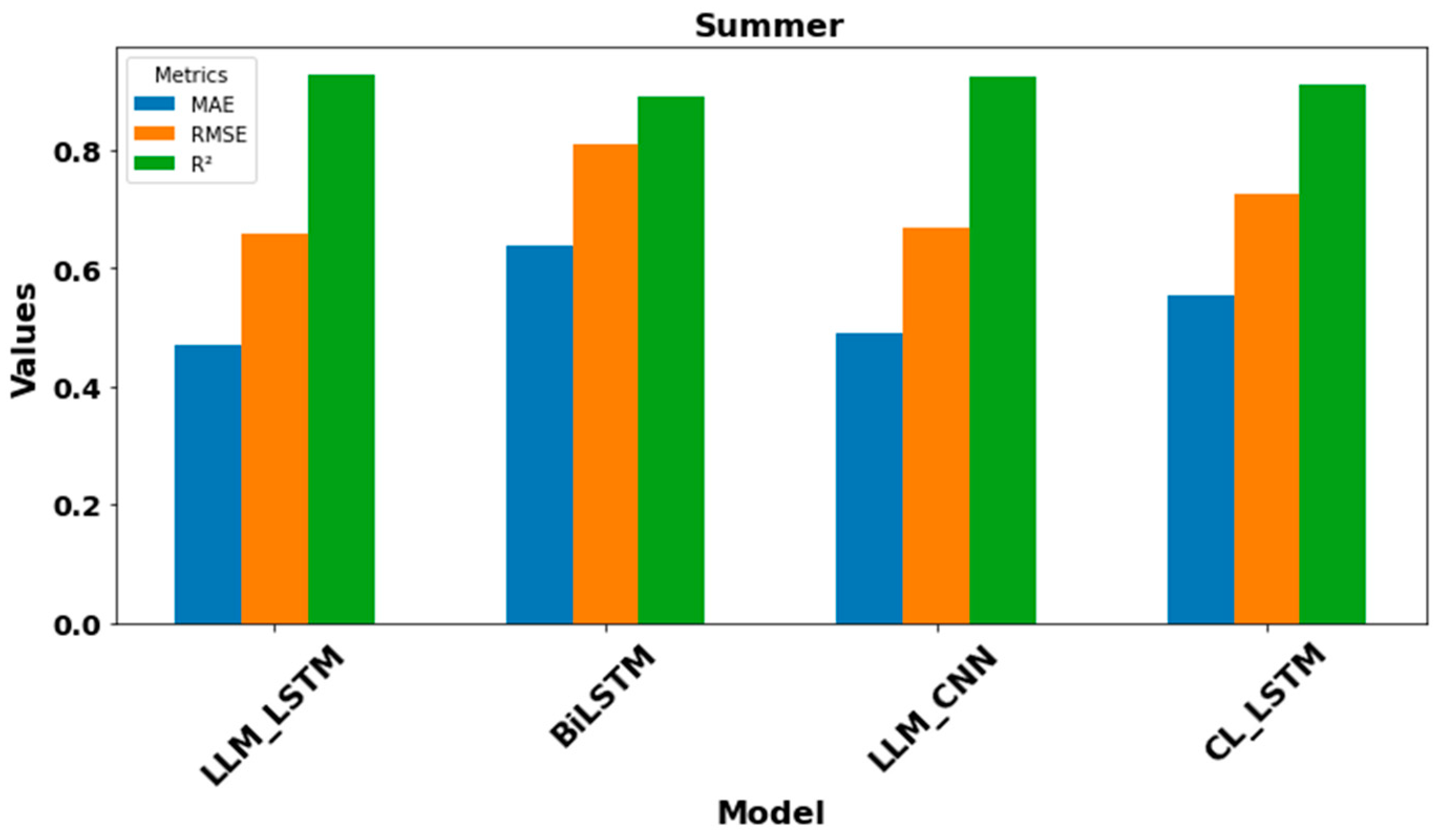
Figure 11.
Linear regression plots for the different methods between actual and predicted values.
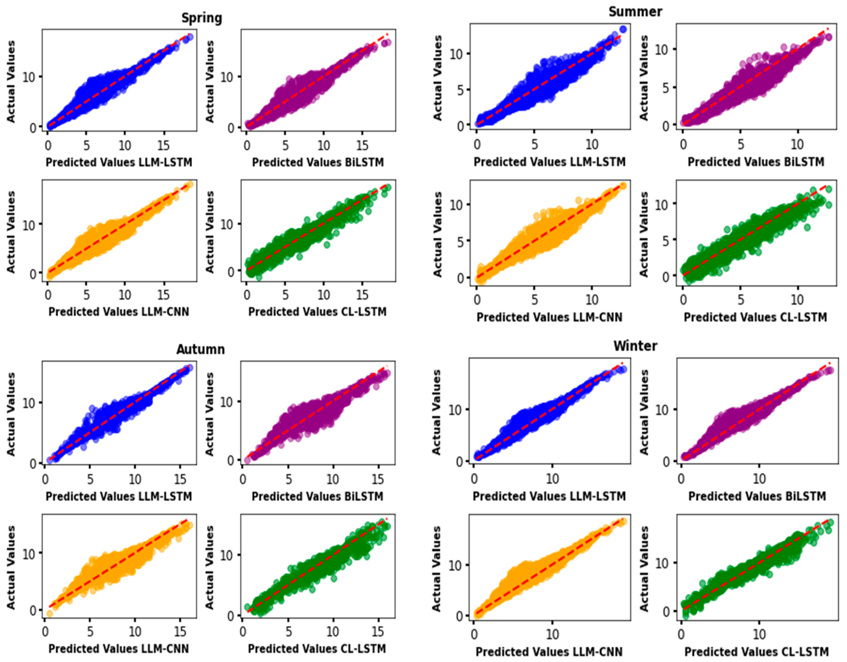
Figure 12.
Presentation of residues from different models for different seasons.
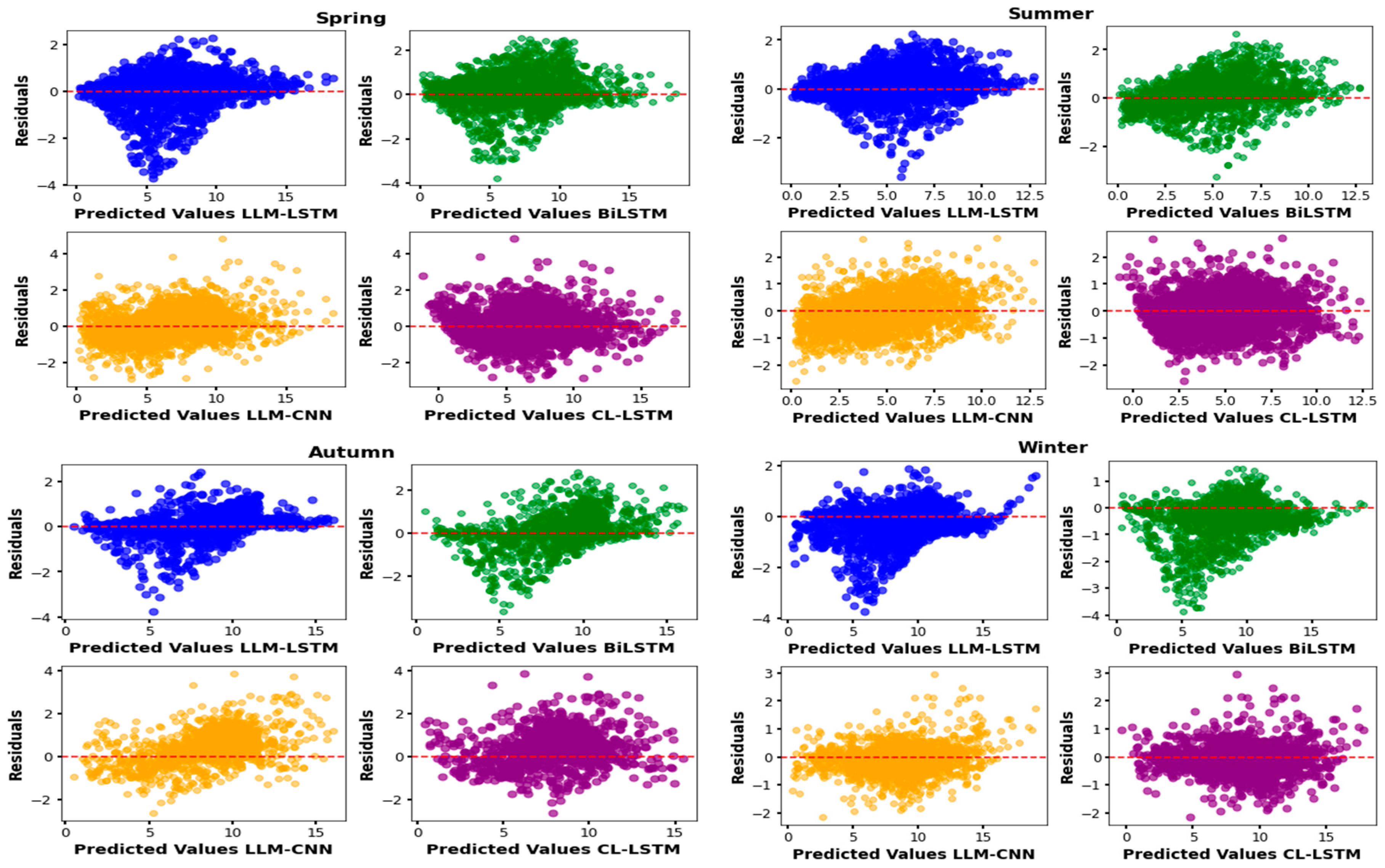
Figure 13.
Four-season wind rose diagram.
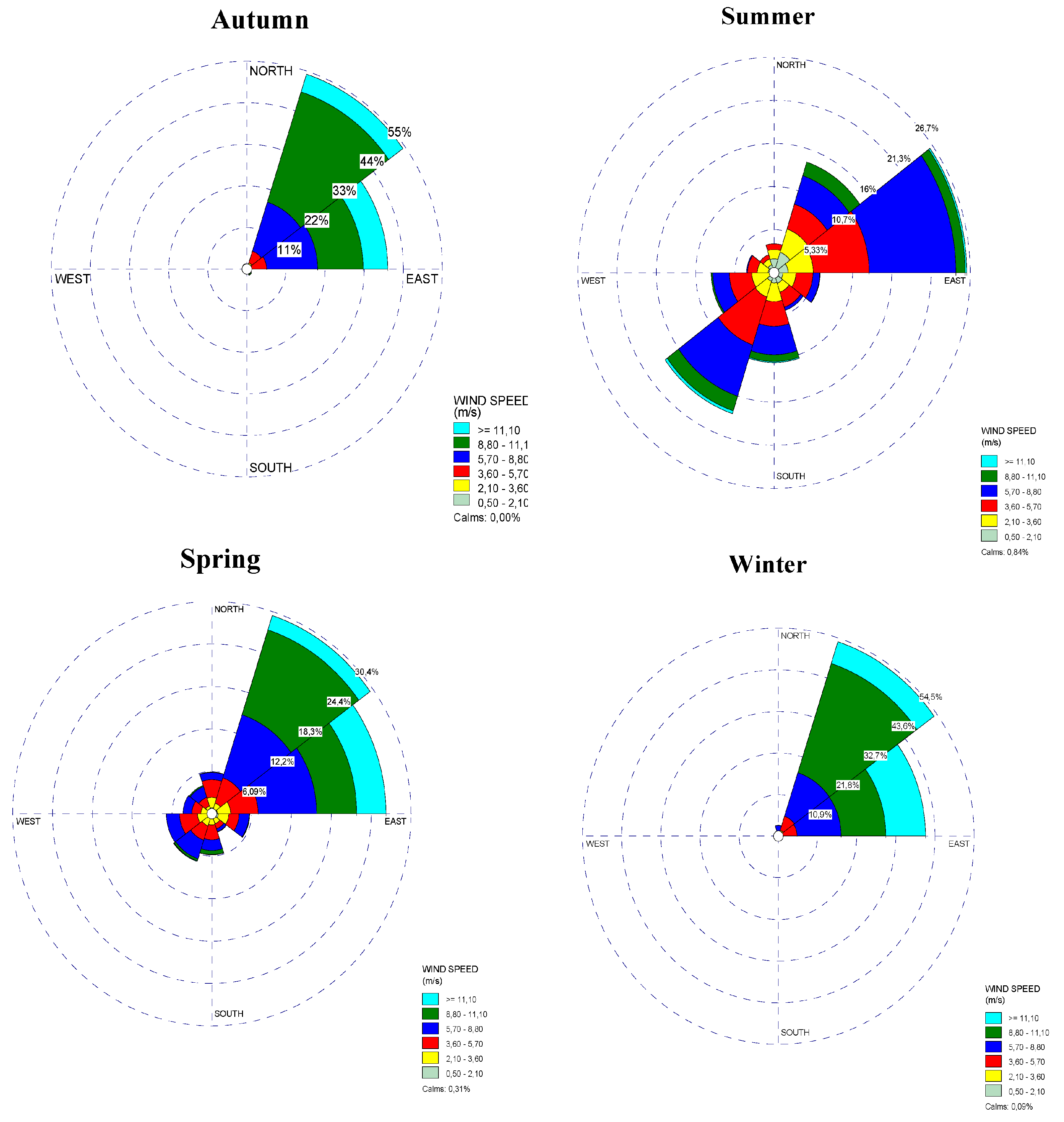
Table 1.
Literature review results.
| Model | MAE (m/s) | RMSE (m/s) | R2 |
|---|---|---|---|
| BiLSTM-CNN [16] | 1.7344 | 2.5492 | 0.9929 |
| CL-LSTM [17] | 1.8983 | 2.7343 | 0.9918 |
| CNN-LSTM [18] | 1.8296 | 2.6307 | 0.9924 |
| BiLSTM [19] | 1.6500 | 2.3000 | 0.9960 |
| CNN-BiLSTM [20] | 0.1042 | 0,1309 | 0.9413 |
| Bi-GRU [21] | 0.0122 | 0.0187 | 0.9887 |
| LSTM-DBN [22] | 0.872 | 1.1055 | 0.8170 |
| CNN-LSTM [23] | 0.512 | 0.703 | 0.7030 |
Table 2.
Correlation coefficients of inputs variables.
| Variables | Correlation Coefficient |
|---|---|
| Temperature | 0.73 |
| Wind direction | -0.64 |
| Relative humidity | -0.55 |
| Atmospheric pressure | 0.78 |
Table 3.
Advantages and disadvantages of each study model.
| Model | Advantages | Disadvantages |
|---|---|---|
| CNN-LSTM | Combines the feature extraction benefits of CNNs and LSTMs for temporal modeling. | Complex to implement and difficult to optimize. |
| BiLSTM | Captures dependencies in both forward and reverse directions; less sensitive to variations and noise in the data. | Computationally more complex and time-consuming than simple LSTMs. |
| Cl-LSTM | Incorporates convolutional layers to extract local features before temporal modeling. Effective for data with both spatial and temporal structures. |
More complex to train and tune than simple LSTM models. Computationally time-consuming; may require significant computational resources. |
| LLM-LSTM | Ability to handle large data sequences; good for long-term forecasting. | Very demanding in terms of data resources; complex to implement. |
Table 4.
Summary of statistical measures for evaluation.
| Metrics | Equation | Description |
|---|---|---|
| MAE | (23) | The mean absolute error is a quantity often used to measure the deviation between observed and predicted values. Its mathematical formula is given by equation (23) [35]. |
| RMSE | (24) | RMSE is a measure of the variation of predicted values around measured values. The smaller its value, the better the model. The square root of the mean square error is defined according to formula (24) [35]. |
| R2 | (25) | The coefficient of determination R² is a statistical measure of how closely a model’s predictions match the actual values [36,37]. It is defined by formula (25). |
Table 6.
Overview of evaluation performance values.
| Models | Metrics | Spring | Summer | Autumn | Winter |
|---|---|---|---|---|---|
| LLM-LSTM | MAE | 0.556 | 0.442 | 0.435 | 0.469 |
| RMSE | 0.820 | 0.629 | 0.647 | 0.689 | |
| R2 | 0.932 | 0.933 | 0.939 | 0.940 | |
| BiLSTM | MAE | 0.502 | 0.494 | 0.586 | 0.535 |
| RMSE | 0.745 | 0.686 | 0.812 | 0.740 | |
| R2 | 0.944 | 0.920 | 0.904 | 0.931 | |
| LLM-CNN | MAE | 0.503 | 0.500 | 0.523 | 0.566 |
| RMSE | 0.752 | 0.689 | 0.766 | 0.830 | |
| R2 | 0.943 | 0.919 | 0.914 | 0.914 | |
| CL-LSTM | MAE | 0.636 | 0.531 | 0.628 | 0.020 |
| RMSE | 0.848 | 0.679 | 0.811 | 0.027 | |
| R2 | 0.927 | 0.922 | 0.902 | 0.966 |
Table 8.
Presentation of different values fo V0, K0, C0, FC and E.
| Seasons | V0 | K0 | C0 (m/s) | FC | E (MWh) |
|---|---|---|---|---|---|
| Spring | 8.34 | 3.03 | 9.34 | 0.68 | 4.25 |
| Summer | 5.025 | 2.38 | 6.76 | 0.55 | 0.89 |
| Autumn | 8.42 | 3.05 | 9.42 | 0.68 | 4.10 |
| Winter | 8.95 | 3.14 | 10.00 | 0.69 | 4.91 |
Disclaimer/Publisher’s Note: The statements, opinions and data contained in all publications are solely those of the individual author(s) and contributor(s) and not of MDPI and/or the editor(s). MDPI and/or the editor(s) disclaim responsibility for any injury to people or property resulting from any ideas, methods, instructions or products referred to in the content. |
© 2025 by the authors. Licensee MDPI, Basel, Switzerland. This article is an open access article distributed under the terms and conditions of the Creative Commons Attribution (CC BY) license (http://creativecommons.org/licenses/by/4.0/).
Copyright: This open access article is published under a Creative Commons CC BY 4.0 license, which permit the free download, distribution, and reuse, provided that the author and preprint are cited in any reuse.


