Submitted:
17 April 2025
Posted:
18 April 2025
You are already at the latest version
Abstract
A statistical field model is constructed on Minkowski spacetime for a self-interacting Dirac field that fluctuates with respect to an auxiliary parameter. The fluctuating Dirac field undergoes a variational Hamiltonian flow while exchanging action with an action bath. Assuming ergodicity, the partition function is calculated and used to provide a perturbative expansion for the field's correlation functions. Non-perturbative calculations are carried out and the resulting 2-point correlation functions have a distinct light cone structure as expected for a relativistic field theory.
Keywords:
Relativistic statistical field theory
Introduction
Traditionally, non-perturbative quantum field theory calculations are performed on Euclidean lattices [1,2,3]. Physics, however, is relativistic. Euclidean lattice models lack a unique time-like direction and instead rely on analytical continuation to connect the Euclidean correlation functions to observables on Minkowski spacetime [3,4,5]. While several methods are known for generalizing these reconstructions to some curved spactimes, it would still be desirable to have models formulated on spacetime directly [6,7,8,9]. For this reason, various “real-time” methods have been developed to non-perturbatively calculate correlation functions directly on Minkowski spacetime. Many of these real-time models, however, face convergence issues because the actions of quantum field theories are usually not bounded from below and because fields are often weighted by a complex phase factor [10,11]. Other authors have addressed some of these issues using various relativistic statistical field theory constructions [12,13,14,15,16].
Recently, however, the present author has developed a statistical field model with two key features: (1) a relativistic action that is bounded from below and (2) an extended variational phase space whereby the fluctuating fields exchange action with an action bath [17]. Assuming ergodicity, the combination of these two features provides a relativistic partition function that samples a canonical ensemble of field configurations. The present article refines this approach and applies in to an interacting Dirac field model.
Preliminaries
The action of the free Dirac equation is typically expressed as where I is the 4x4 identity matrix, , and with denoting the Dirac representation gamma matrices and providing coordinates on Minkowski spacetime. To get the classical equations of motion for , one usually sets the variational derivative of the action with respect to equal to zero; however, one could equivalently set the variational derivative with respect to equal to zero to afford . Often, it is more efficient to deal with the momentum space version of the Dirac equation where, after Fourier transformation, the partial differential equations become the matrix equation where now . The matrix is diagonalizable. Diagonalizing this matrix gives where is the diagonal matrix defined in equation (1) with and is an invertible matrix.
The diagonalization of a matrix describes, in a different basis, the same operator as the original matrix. Redefining the Dirac field in this new basis as , the Dirac equation is now expressed as . Using the inverse Fourier transformation then gives the spacetime representation of this diagonalized Dirac equation as the pseudodifferential equation where . This diagonalized Dirac operator is conceptually similar to the pseudodifferential operator square root of the Klein-Gordon equation described previously by Lämmerzahl [18]. Indeed, one can define an adjoint operator that composes with D to give the Klein-Gordon equation. To see this, return to the free Dirac action and this time set the variational derivative with respect to to zero to get . Taking the Hermitian conjugate of both sides gives . The momentum space representation of the matrix is again diagonalizable and affords the diagonal matrix defined in Equation (2).
Composing with gives . It follows that as desired. Because the original basis for the Dirac field is unimportant, the tick mark, ′ , will be dropped from the notation going forward and will be understood to be a collection of four complex-valued fields , .
These diagonalized free Dirac equations are interesting because one can define smooth, positive-definite integral kernels that are approximate solutions. For example, define according to:
where is a small positive number and are defined as follows:
The integral kernel is an approximate solution of the diagonalized free Dirac operator D in the sense that because:
since approaches a Dirac delta distribution centered on as .
Moreover, is positive-definite because each of is. That is, for any complex-valued function h, with complex conjugate , that is not identically zero, these integral kernels have the following property:
This property follows from the Plancherel theorem [19] whereby is equal to and everywhere when .
The integral kernels also have smooth, closed form spacetime representations which can be found by explicitly evaluating the Fourier integrals. First, evaluate the integral with respect to to get:
Switching to spherical coordinates with , , and gives:
The integral with respect to the angle can be performed to give1:
According to the Bateman Table of Integral Transforms at page 75, equation 36 [21], this integral has the following closed-form solution:
where is the modified cylindrical Bessel function of the second kind and order one.
With these properties, encodes the physics of the free Dirac equation into a smooth, positive-definite integral kernel with a closed-form spacetime representation.
Constructing the Statistical Dirac Field Model
Let X denote a simply connected region of Minkowski spacetime having a boundary, , and finite 4-volume, . The Dirac field, , is a collection of four complex-valued scalar fields, , on X that is typically arranged in column vector notation as:
Suppose that this Dirac field “fluctuates” with respect to some parameter . The variation of for any given value of is defined as . To prescribe physics to these fluctuations, it is useful to couple to an additional fluctuating field defined as:
where each is a complex-valued scalar field. Fluctuations of are defined by . As these fields fluctuate, they can exchange action with an action bath by interacting with the action bath parameter which is a global, real-valued parameter with . The action bath parameter will likewise be coupled to an additional parameter denoted by with . Together, these fields define the degrees of freedom of the system. To define how these fields fluctuate consider the following action:
Here, , , , and q are real-valued constants that do not depend on and the explicit -dependence of the degrees of freedom is omitted in favor of a more compact notation. The constant in particular is defined such that . In , the term is the operator inverse of and necessarily exists and is positive-definite because is positive-definite. The operator inverse is used here so that the 2-point correlation function of the free field is proportional to as shown in one of the sections below. Additionally, the term is an interaction term for the Dirac field, an example for which is provided in the examples section below. Overall, the term must be bounded from below, and this limitation constrains the set of acceptable interaction terms .
The development of the degrees of freedom with respect to is then defined by the following variational analog of Hamilton’s differential equations:
Here, denotes the variational derivative. These equations define a symplectic flow on the variational phase space consisting of the degrees of freedom. This flow conserves the total action of the system, assuming appropriate boundary conditions, because the total action acts as a variational Hamiltonain [17,22,23,24]. When the fields are discretized for numerical simulation, these variational equations become a finite system of partial differential equations that can be integrated numerical with respect to as demonstrated in the examples section below. Thus, assuming a suitable prescription for all of the degrees of freedom at , one can obtain a 1-parameter family of system configurations from which observables can be calculated.
Observables, Expectation Values, and the Partition Function
The observables of interest for this system are functionals of Dirac field, e.g., . The expectation value of an observable is given by its average with respect to . Specifically, . These expectation values can be computed during numerical simulations. Assuming ergodicity of the system’s dynamics with respect to , one can also calculate expectation values using the partition function.
The partition function is defined by the ergodic average over the variational phase space using the phase space measure given by:
where is the functional integral measure over N discretized points, the other functional integral measures are defined analogously, and C is a normalization constant. Define the following change of variables: and . This change of variables is equivalent to a re-scaling of . See the article by Bond, Leimkuhler, and Laird for an analogous construction used in classical statistical mechanics [25]. This change of variables changes the integration measure in the partition function by a factor of to give:
Recall the identity , where is the isolated zero of . For the systems of interest here, is given by the following equation:
Assigning a unit volume to each of the N points in the functional integral measure gives . Performing the integral with respect to affords:
Now, the integrals with respect to , , are all Gaussian and can be evaluated and, after collecting constant terms, affords the partition function:
The partition function is helpful for calculating expectation values because, by the assumption of ergodicity, the expectation value of some observable taken with respect to agrees with its ensemble average. In equations:
Because the expectation value with respect to agrees with the ensemble average, let denote the expectation value determined by either method.
Correlation Functions
The correlation functions encode the physics of the system. These correlation functions can be calculated perturbatively using the partition function, as demonstrated in this section, or non-perturbatively by numerically integrating the system’s evolution with respect to , as demonstrated in the next section. To begin, consider the cumulant generating function:
where is a source term, and recall the definition of :
The correlation functions are calculated in terms of the cumulant generating function by taking variational derivatives with respect to and followed by setting the source terms to zero:
These correlation functions can be expressed perturbatively in the interaction term, , by expanding them as a series in the parameter q. The generating function can be compactly expressed by making use of the following indentity terms of a variational operator acting on the free partition function as follows:
where the details of this expression can be found in Bailin and Love at Chaper 5 [26]. The free partition function, defined as:
is a standard Gaussian integral which can be evaluated to give:
Combining the above equations, the correlation functions can be expressed in terms of various contractions of the integral kernel , and one could use a diagrammatic technique similar to the Feynman diagrams to keep track of these terms. In particular, this shows that the 2-point correlation function of the free field is given by:
Examples
An advantage of the model developed in the previous sections is that it is easy to discretize and simulate numerically. In each of the following examples, the field was evaluated on a set of 4096 points selected at random from the region X of Minkowski spacetime that satisfies and for each with a uniform distribution of points in the (t, r) plane. Each component of and was initialized with a random phase and magnitude ranging from -1.75 to 1.75. The variables s and where initialized to 1 and 0, respectively. The parameter values and were used. The value of was set to 0.01 for the integral kernel, , and the integral kernel was divided by its value at to standardize the results.
Once an initial configuration was established, each example was numerically integrated with respect to using the explicit leap-frog algorithm provided by Bond, Leimkuhler, and Laird [25] with a step size of . Each system was “equilibrated" by stepping the system forward for 1,000,000 steps. After this “equilibration” period, each system was further numerically integrated with respect to for an additional 5,000,000 steps during which data was collected. The collected data included expectation values of the form where and with being a set of 225 equally sized, real-valued functions that tesselate X by taking the value 1 in a triangularly supported region of the (t, r) plane and taking the value 0 outside of each function’s respective region of support. Further, covers the origin where (t, r)=(0, 0).
Example 1: Free Field
In this example, the free field model was used (i.e., q=0). The real and imaginary parts of the expectation value were each normalized to a maximum absolute value of 1 and are ploted in Figure 1A and 1B, respectively. From the calculation of the 2-point correlation function in the previous section, one would expect to approximate which is to proportional to . Moreover, which is the Pauli-Jordon propagator.
As seen in the plot of the imaginary part (Figure 1B), the correlation function has three distinct regions: (I) the interior of the past-directed light cone, (II) the acausal region, and (III) the interior of the future-direct light cone. Regions, (I) and (III) have a small oscillatory character whereas region (II) is substantially zero. Moreover, region (II) is separated from regions (I) and (III) by a sharp light cone with the past-directed light cone and future-direct light cone being antisymmetric with respect to time inversion. All of these properties are consistent with the expectation that the result should be similar to the Pauli-Jordon propagator.
The real-part of the correlation (Figure 1A), by contrast, is more noisy with a large negative feature near the origin and some smaller oscillatory behavior in the interiors of the future and past directed light cones. These effects may be due to the non-interacting nature of the separate modes which do not cancel each other out to give zero. This hypothesis is supported in the following interacting model wherein the real part of the correlation function is substantially feature-less noise.
Example 2: Interacting Model
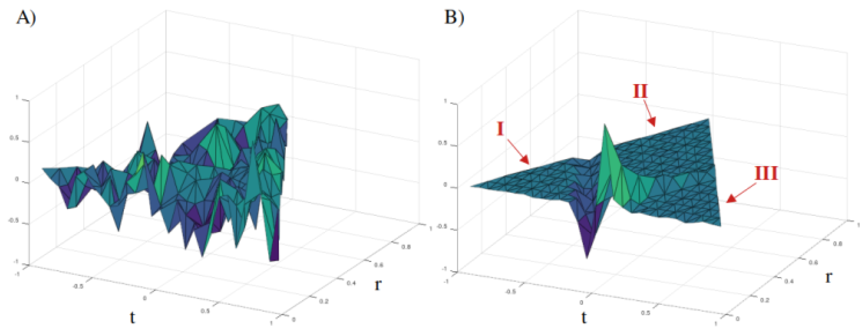
In this model, the following interaction term was used with q=0.1:
Here, the and terms are currents generated by the fluctuating Dirac field and they interact through the time-symmetrized integral kernel and its complex conjugate where additionally parameterizes a small but positive mass term that, in the limit as goes to zero, may mimic the exchange of a photon. The interaction kernel was found to be positive-definite by Cholesky decomposition for the system under consideration; so, other interaction models could consider using an inverse of this kernel. The factor was included to standardize the magnitude.
As seen in the plot of the imaginary part (Figure 2B), the correlation function has three distinct regions: (I) the interior of the past-directed light cone, (II) the acausal region, and (III) the interior of the future-direct light cone. Regions, (I) and (III) have a small oscillatory character whereas region (II) is substantially zero. Moreover, region (II) is separated from regions (I) and (III) by a sharp light cone with the past-directed light cone and future-direct light cone being antisymmetric with respect to time inversion. These properties suggest that this interacting model may obey causality as would be required for a physically meaningful model.
The real-part of the correlation (Figure 2A), by contrast, looks like feature-less noise. While both plots were normalized to have a greatest absolute value of 1, before normalization the maximum absolute value for the real part was about two orders of magnitude smaller than that of the imaginary part. This suggests that the real part may be effectively zero.
Discussion
These results demonstrate an implementation of a statistical Dirac field model on Minkowski spacetime. The 2-point correlation functions of both the free field model and the interacting model have light cone structures similar to what one would require from a relativistic field theory. Future work may involve attempting to construct a fermionic algebra of observables with the appropriate anti-commutation relations.
References
- Roepstorff, G. Path integral approach to quantum physics: an introduction; Springer Science & Business Media, 2012.
- Montvay, I.; Münster, G. Quantum fields on a lattice; Cambridge University Press, 1994.
- Glimm, J.; Jaffe, A. Quantum physics: a functional integral point of view; Springer Science & Business Media, 2012.
- Osterwalder, K.; Schrader, R. Axioms for Euclidean Green’s functions. Communications in mathematical physics 1973, 31, 83–112. [CrossRef]
- Osterwalder, K.; Schrader, R. Axioms for Euclidean Green’s functions II. Communications in mathematical physics 1975, 42, 281–305. [CrossRef]
- Ashtekar, A.; Marolf, D.; Mourao, J.; Thiemann, T. Osterwalder-Schrader reconstruction and diffeomorphism invariance. arXiv preprint quant-ph/9904094 1999.
- Visser, M. How to Wick rotate generic curved spacetime. arXiv preprint arXiv:1702.05572 2017.
- Baldazzi, A.; Percacci, R.; Skrinjar, V. Wicked metrics. Classical and Quantum Gravity 2019, 36, 105008. [CrossRef]
- Schrader, R. Reflection positivity in simplicial gravity. Journal of Physics A: Mathematical and Theoretical 2016, 49, 215202. [CrossRef]
- Berges, C.E.; Rammelmuller, L.; Loheac, A.C.; Ehmann, F.; Braun, J.; Drut, J.E. Complex Langevin and other approaches to the sign problem in quantum many-body physics. Physics Reports 2021, 892, 1–54. [CrossRef]
- Berges, J.; Borsanyi, S.; Sexty, D.; Stamatescu, I.O. Lattice simulations of real-time quantum fields. Physical Review D 2007, 75, 045007. [CrossRef]
- Giachello, M.; Gradenigo, G. Symplectic quantization and the Feynman propagator: a new real-time numerical approach to lattice field theory. arXiv preprint arXiv:2403.17149 2024.
- Tilloy, A. Interacting quantum field theories as relativistic statistical field theories of local beables. arXiv preprint arXiv:1702.06325 2017.
- Floerchinger, S. Quantum field theory as a bilocal statistical field theory. arXiv preprint arXiv:1004.2250 2010.
- Hitschfeld, B.S. Probability Density Functionals in Perturbation Theory within the QFT in-in Formalism. arXiv preprint arXiv:1901.09734 2019.
- Kent, A. Path integrals and reality. arXiv preprint arXiv:1305.6565 2013.
- McDearmon, B. A relativistic statistical field theories on a discretized Minkoski lattice with quantum-like observables. arXiv preprint arXiv:2405.2038 2024.
- Lämmerzahl, C. The pseudodifferential operator square root of the Klein-Gordon equation. Journal of mathematical physics 1993, 34, 3918–3932. [CrossRef]
- Rudin, W. Functional Analysis; McGraw-Hill, 1973.
- Scharf, G. Finite quantum electrodynamics: the causal approach; Courier Corporation, 2014.
- Bateman, H.; Erdélyi, A.; Magnus, W.; Oberhettinger, F. Tables of integral transforms 1954. 1.
- McDearmon, B. A momentum space formulation for some relativistic statistical field theories with quantum-like observables. arXiv preprint arXiv:2406.04365 2024.
- McDearmon, B. Euclidean Quantum Field Theory from Variational Dynamics. arXiv arXiv:2303.12666 2023.
- McDearmon, B. Euclidean Quantum Gravity from Variational Dynamics. arXiv arXiv:2302.05713 2023.
- Bond, S.D.; Leimkuhler, B.J.; Laird, B.B. The Nose-Poincare method for constant temperature molecular dynamics. Journal of Computational Physics 1999, 151, 114–134. [CrossRef]
- Bailin, D.; Love, A. Introduction to Gauge Field Theory Revised Edition; Taylor & Francis, 1993.
| 1 | A similar integral is evaluated in spherical coordinates in the book by Sharf at equations (2.3.8) and (2.3.9) [20]. |
Figure 1.
Normalized real part (A) and imaginary part (B) of the correlation function of the free field model in the (t, r) plane. Before normalization, the maximum absolute value for the real part was 0.8 times that of the imaginary part.
Figure 1.
Normalized real part (A) and imaginary part (B) of the correlation function of the free field model in the (t, r) plane. Before normalization, the maximum absolute value for the real part was 0.8 times that of the imaginary part.
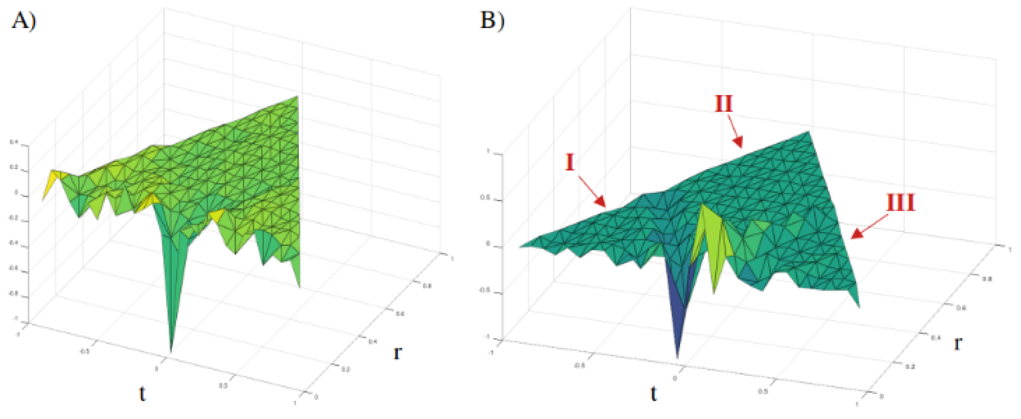
Figure 2.
Normalized real part (A) and imaginary part (B) of the correlation function of the interacting field model in the (t, r) plane. Before normalization, the maximum absolute value for the real part was 0.018 times that of the imaginary part.
Figure 2.
Normalized real part (A) and imaginary part (B) of the correlation function of the interacting field model in the (t, r) plane. Before normalization, the maximum absolute value for the real part was 0.018 times that of the imaginary part.
Disclaimer/Publisher’s Note: The statements, opinions and data contained in all publications are solely those of the individual author(s) and contributor(s) and not of MDPI and/or the editor(s). MDPI and/or the editor(s) disclaim responsibility for any injury to people or property resulting from any ideas, methods, instructions or products referred to in the content. |
© 2025 by the author. Licensee MDPI, Basel, Switzerland. This article is an open access article distributed under the terms and conditions of the Creative Commons Attribution (CC BY) license (https://creativecommons.org/licenses/by/4.0/).
Copyright: This open access article is published under a Creative Commons CC BY 4.0 license, which permit the free download, distribution, and reuse, provided that the author and preprint are cited in any reuse.


