
Submitted:
16 April 2025
Posted:
18 April 2025
You are already at the latest version
Abstract
This paper elucidates the Lorentz group, a fundamental subgroup of the Poincaré group. The orbits and little groups associated with the Lorentz group are described in detail, along with their corresponding properties. The Poincaré group is presented. Another of the fundamental aspects of the Poincaré group is Wigner's little groups obtained from this group. An in-depth discussion both for the cases of massive and massless relativistic particles within the context of little groups is given. Our examination extends to the properties of various special groups associated with the Poincaré group. Applications of these groups are elaborated by physical examples taken from high-energy physics and optics from both classical and quantum domains. Specifically, covariant harmonic oscillators including entangled states, proton form factors, and the parton picture as proposed by Feynman are discussed. In this context, laser cavities and shear states are also addressed. We lay out the underlying mathematics that connects these apparently disparate realms of physics.

Keywords:
lorentz group
; Poincaré group
; little groups
; covariant harmonic oscillators
; proton form factors
; Feynman's parton picture
; laser cavities
; quantum shear states
1. Introduction
It had long been thought that one promising approach to unifying special relativity and quantum mechanics was to develop a covariant formulation of quantum field theory. This however, has not been the only approach. Indeed, P.A.M. Dirac in his 1949 paper [1], suggested that the construction of a representation of the Poincaré group (alternatively called the inhomogeneous Lorentz group) might be the right place with which to begin. For studying the Poincaré group, Wigner’s 1931 book on atomic spectra, containing many physical ideas, as well as the paper he wrote in 1939 on the inhomogeneous Lorentz group [2,3] provide a good starting point.
The limitations of formulating a covariant quantum field theory became apparent when the extended charge distribution of the proton [4] was discovered and the subsequent formulation of the quark theory [5,6,7]. Considering that quarks are permanently confined inside hadrons, any theory unifying special relativity and quantum theory has to account for the bound state of quarks inside the hadron.
We contend that the same space-time symmetry should be inherent in any bound-state model. One of the purposes of this paper is to show that the principles contained in Wigner’s 1939 [2] paper and in Dirac’s 1949 [1] paper provide us the means to build a relativistic bound-state model that can explain the features of hadrons currently observed in high-energy laboratories.
It was Wigner who in 1927 [8] introduced group theory into physics. In the present time, there is more and more interest in constructing explicit representations of groups that are now used in physics. Most of the groups used in physics are Lie groups. They provide a better understanding of physical phenomena through symmetries in almost all branches of physics. It is well known that the angular momentum and the spin operators are described by the rotation group and in quantum mechanics [9]. Almost all gauge theories rely on Lie groups and the associated Lie algebras [10], including the Lorentz and Poincaré groups [11] addressed in this paper. Likewise, particle physics utilizes these formulations for the space-time symmetries of relativistic particles [12,13,14]. Classical and quantum optics are no exceptions to this enterprise [15]. It is also worthwhile to mention a completely different field from those we shall discuss here, namely statistical mechanics and thermodynamics [16,17].
A Lie group, is a group which is also a smooth manifold, where the group operations, specifically the multiplication and the inversion are both smooth maps. A closed set of generators, as we shall see below, determines the properties of Lie groups. This closed set is entitled the Lie algebra of the group.
One can obtain the Lie group from the Lie algebra by exponentiation. Consider any complex valued square matrix such as X then
From this the group element the correspondence to any parameter can be derived from
The algebra of a particular Lie group can be obtained by differentiation
In Section 2 we review Lorentz transformations which have become the bedrock formulation for special theory of relativity. We present the Lie algebra and give a representation in terms of the four-by-four matrices that result from it. We further present the little groups of the Lorentz group and the orbits that are also associated with this group. In Section 3, we show that the group of Lorentz transformations has a covering group, known as .
Section 4 consists of a discussion of the subgroups contained in the Lorentz group which itself is a subgroup of the Poincaré group. Specifically, we examine the subgroups , the covering group , along with , and . These groups are special groups, all having det(+1). On the other hand, we note that has two connected components, one with det(+1) and the other with det(-1). Reflections belong to , but not to . The Lie algebra obtained from the connected component to the identity is the same as the Lie algebra obtained from , however, this algebra does not encompass the other connected component of having det(-1).
Section 5 presents the Poincaré group and representations of the Poincaré group are constructed. We then discuss Wigner’s little groups that are the subgroups of the Poincaré group. In addition to the little groups discussed in Section 2, specifically, the group and the group for massive and imaginary mass particles, here we note that there exists an -like subgroup of the Poincaré group for massless particles. We also give the two-by-two representations of these little groups to the end that and become the -like and the -like groups of Wigner [2]. Although it is well-known that the rotational symmetry governed by the -like group corresponds to the helicity of the photon, translational degrees of freedom of this group needed to be elucidated further. This section also clarifies the physical meaning of these translational degrees of freedom.
In Section 6 we give physical examples where the mathematics described in the preceding sections is used. In 1949 [1], Dirac suggested that finding a representation of the Poincaré group is to be undertaken by Lorentz-covariant quantum mechanics. In that regard, a formalism for covariant harmonic oscillators that is compatible with Dirac’s general strategy to develop a relativistic quantum mechanics is rendered. Thus, we show how the Lorentz group is manifested through coupled covariant harmonic oscillators. In that context we discuss the proton form factor, which is an ongoing research in high-energy physics, both theoretically and experimentally. For that matter, we discuss quarks and Feynman’s partons as being two different manifestations of the same covariant entity. We also give two more applications from classical and quantum optics, namely resonators in laser cavities and quantum shear states, respectively.
2. The Lorentz Group
We start by considering the four dimensional spacetime manifold with coordinates
Conventionally, Lorentz transformations are defined to be the group that preserve the inner product , with , where the Minkowski metric is taken to be . Specifically we have
where stand for the components of the transformation matrix. This group is called when Lorentz transformations are restricted to being proper, i.e., to the condition that . Here they will also be constrained by . This is known as the proper orthochronous Lorentz group.
When transformations are applied to the column vector , the matrix form of the generators is:
They form six independent generators for the Lie algebra of the Lorentz group.
The transformation matrices of the Lorentz group can be written in exponential form:
Here are the generators of rotations and are proper Lorentz boosts. In the Appendix we tabulate the explicit matrix forms for each transformation matrix obtained through exponentiation: and .
Generally, when considering the generators above which form the Lie algebra of the Lorentz group one can apply them to an arbitrary coordinate variable function:
with and . These generators satisfy these commutation relations:
The first commutator shows that the are indeed the generators of the rotation subgroup of , the proper Lorentz group. The second and third commutators indicate that the boosts by themselves do not form a group. Multiplying two pure boosts will produce both a boost and a rotation.
We can combine the six generators shown in Equation (8) into the covariant form
where
Considering transformations on and , behaves like a second-rank tensor
when a Lorentz transformation is applied. Then for commutation relations are [18]:
2.1. Orbits of the Lorentz Group
Let X be a vector space and p a point in that vector space. Now, if is a group, then the little group of G at p is the maximal subgroup leaving p invariant. The orbit of G at p is the set of points V that can be reached applying G to the single point p in X.
The little groups of the proper Lorentz group are a subset of transformations , which leave the four-vector invariant
The orbits of proper Lorentz group the are such that
generating surfaces in this four dimensional space. Here, is identified as the four-momentum and written as a column vector .
The four-momentum is either time-like , light-like or space-like . By analyzing the little group for a single typical four-vector on each orbit, these orbits allow us to investigate every potential little group.
When considering the proper Lorentz group, six orbits can be distinguished. Two time-like surfaces that have positive compose the first two orbits. These have, respectively, positive and negative values of . The forward and backward light cones, respectively, constitute the third and fourth orbits. The fifth orbit has negative values of and therefore is a space-like surface. The sixth orbit, where , is the origin in this space.
The linear equations in Equation (14) have to be solved so as to find representations of the little groups such that for each representative , the transformation matrix is to satisfy Equation (5). The number of independent parameters is reduced by this latter condition to three.
- (a)
- For time-like : We have . The little group is thus the rotation group.
- (b)
- For light-like : This four-vector is invariant under rotations around the z-axis.
- (c)
- For again light-like : the rotation matrix is the same.
- (d)
- For space-like : This four-vector remains invariant under rotations around the z-axis as well as boosts along either the x and y-axis. Together, these form the three-dimensional Lorentz group satisfying the required condition.
- (e)
- For : The entire Lorentz group leaves this zero momentum invariant, where the origin is the orbit.
These orbits are shown in Figure 1.
To be used later in Section 6, we give a particular little group transformation for a relativistic massive particle moving in the z-direction whose initial four-momentum is . When boosted back to its rest frame with , it takes the form , with . Then in the rest frame this can be rotated around the y-axis, where we make use of the respective boost and rotation matrices in the Appendix. Finally, it is boosted to its initial momentum with . The chain of process yields
which is a little group transformation.
We shall discuss in Section 5, the little groups of the Poincaré group. There we shall see that not all the little groups of the Poincaré group coincide with the little groups of the Lorentz group, due to the fact that the Lorentz group is a subgroup of the Poincaré group.
3. The Covering Group of the Lorentz Group: SL(2, c)
Let us consider the group generated by the following six two-by-two matrices:
where are the Pauli spin matrices defined as
The explicit forms of the operators in Equation (17) are
These matrices satisfy the commutation relations:
These relations are identical to those of the Lorentz group. is homomorphic (the mapping is onto but not one-to-one) to , namely it is the double cover of .
The group of two-by-two matrices whose generators are defined in Equation (17) is of the form
and has the same algebraic properties as that of the Lorentz group. Specifically, matrices in Equation (17) are the generators of the group. These generators are traceless, so the determinant of W is one. Therefore, is an unimodular (det = 1) group. On the other hand, is not a unitary group, given that the matrices are not Hermitian. We point out that if the sign of is changed in Equation (20) the Lie algebra remains invariant. In the case of , the sign of the boost generators is unambiguously defined in terms of the space and time variables. However, when it comes to , one has to consider both signs. Since the sign change can be easily implemented, the positive sign as given in Equation (19) will be used, unless otherwise required.
Now, we examine the expression of Equation (21) and note that is just i times . Thus, W of Equation (21) can be rewritten as
where . This implies that, three generators and three complex parameters are sufficient to work with the group.
In order to see that matrices belonging to indeed perform Lorentz transformations, we consider the two-by-two coordinate matrix
where is the two-by-two unit matrix. Then
is the quadratic form which should remain invariant. The group elements act on X through the following transformation
Since W and are unimodular, is preserved. Therefore, transformations of the form above are Lorentz transformations.
4. Subgroups of the Lorentz Group
In this section, we give the subgroups of the Lorentz group. For this purpose, it is sufficient to look at the generators of Lorentz group in Equation (6) and investigate which of those can be grouped together to form a closed set.
First, we note that the rotation generators form a closed set, and therefore they constitute a subgroup, namely the or the proper rotation group. These generators are Hermitian, while the boost generators are not.
Now, we consider the two-by-two representation of the Lorentz group, specifically the group. The subgroup is a three parameter group and is generated by the Pauli spin matrices. The generators in Equation (17) satisfy the well-known commutation relations:
Just like the group is to , the group is the double cover of . If W in Equation (25) is restricted to the group, then the t variable is not effected, so the transformation acts only on and is equivalent to a rotation in the three-dimensional space. It is known how the group acts on spinors through unitary transformations that correspond to rotations in the spin space.
Additionally, Lorentz transformations along the x- and y-directions and of the rotation on the -plane around the axis perpendicular to this plane form the group . The generators of this group are , and , as given in Equation (6). They satisfy the commutation relations:
It can also be observed from Equation (19) that , and satisfy the commutation relations:
Since these generators are pure imaginary, the transformation matrices have real elements. This is the two-dimensional symplectic group . Alternatively stated, it is the group. The groups and are locally isomorphic.
From Equation (19) we choose
These are the generators of the group . They satisfy the same commutation relations as those of Equation (27). So, the groups and are also locally isomorphic.
As for the final set of generators, we choose , and . Their commutation relations satisfy
where the group they generate is recognized as an -like group.
4.1. The Squeeze-Rotation and the Shear-Squeeze Representations of the Sp(2) Group
At this point, it is worthwhile to give the squeeze-rotation representation of the group. The generators are given as:
Now we consider:
then we have
They satisfy the commutation relations:
Shear transformation matrices can be decomposed as:
with
This is another representation of the group. This particular representation is called the shear-squeeze representation. This representation builds the necessary algebraic structure of and matrices of classical optics that we shall give in Section 6.3, as well as the quantum shear states provided in Section 6.4.
5. Poincaré Group and Wigner’s Little Groups
Here we define the Poincaré or inhomogeneous Lorentz group. This group consists of both translations and the Lorentz group. It was Eugene Wigner in his landmark 1939 paper [2] who first discussed the little groups that are subgroups of the Poincaré group. The little groups are defined as those groups whose transformations leave the four-momentum of the relativistic particle unchanged.
5.1. Poincaré Group
The Poincaré group is composed of the group of inhomogeneous Lorentz transformations that operate on the four-dimensional Minkowski space in the following form
Here, is the Lorentz transformation matrix defined in Section 2, while consists of the translation parameters. A typical five-by-five transformation matrix applicable to the column vector is of the form
The commutation relations for generators of the Poincaré group are given as [18]:
Here, are the generators of the Lorentz group, while are translation generators. Since does not commute with the Poincaré group cannot be expressed as a direct product of the Lorentz and translation groups. However, the Lorentz group is a subgroup of the Poincaré group.
The generators of the Poincaré group are composed of the generators of the Lorentz group given in Equation (10), together with the translations generated by
5.2. Wigner’s Little Groups
Wigner’s little groups are the subgroups of the Poincaré group whose transformations leave the four-momentum of a relativistic particle invariant. In addition to the Lorentz group, the Poincaré group involves translations. As a preparation to Wigner’s little groups, we first consider the Euclidean or group consisting of translations and a rotation in a two-dimensional Euclidean plane. The transformation equations are defined as [11]:
Translations in the -plane are represented by the parameters u and v.
The generators of this group satisfy
where and generate translations along the x and y-directions, respectively.
We observe that not all little groups of the Poincaré group coincide with the little groups of the Lorentz group. In addition to the little groups we have presented in Section 2.1, which are explicitly given in items , namely the rotation group and the group for massive and imaginary mass particles, for massless particles with there exists a translation-like subgroup of an -like group, whose matrix is in the following form [2]:
Furthermore, there is the Hermitian conjugate of this matrix to be employed when
.
In view of Equation (3), the expressions for the generators of translations, and , can be obtained by taking the derivative with respect to u and v of Equation (47) separately and evaluating at zero. They can be formed through a particular combination of the generators of the Lorentz group as given in Equation (6) in the following way
The little group obtained from the above generators is a subgroup of the Poincaré group. The commutation relations of and are identical to those of the group given in Equation (46). Specifically, they constitute the Lie algebra of an -like group.
Einstein’s special theory of relativity was introduced for point-like particles without any internal structures. On the other hand, in addition to governing the symmetries of the four-momentum Wigner’s little groups also dictate the internal space-time symmetries of relativistic particles. For that matter, for instance for spin massless particles, it is the little group obtained from generators of the following the formulation of Equation (48). However, since all types of neutrinos have been observed to have non-zero mass [19], we are still on watch for the existence of massless spin particles.
On the other side of the coin, photons as being spin 1 particles can safely be regarded to be the most fundamental particle in almost all branches of physics. When it comes to massless particles one is bound to deal with the fact that, there are no Lorentz frames in which they are at rest. Therefore, to be able to tackle this issue we are compelled to go beyond the Lorentz group and consider E(2)-like little groups of the Poincaré group.
For this purpose we consider the transformation having the form
We see here that is invariant under this transformation, but that z can vary from to . Therefore, this defines a cylindrical transformation. It requires little effort to explain the rotational degree of freedom as the helicity of the photon. The interpretation of the translational degrees of freedom has been given in [20,21,22,23] as the gauge degrees of freedom for the photon. The physical aspect of this transformation is illustrated in Figure 2.
Again we resort to [2] to elucidate on the gauge transformation and consider the matrix
where and are as given in Equation (48) . This acts on the four-potential of a photon moving along the z direction. The Lorentz gauge condition yields , then the four-potential becomes
Subsequently, leads to the invariance of and , while the component becomes:
This expression clearly lays out as to how and are involved in gauge transformations.
5.3. Wigner Four-Momentum-Matrices
In addition to massless particles there are also massive and imaginary mass particles. When a massive particle is at rest, Wigner observed that the particle still has three rotational degrees of freedom. Therefore, the rotation group defined in Section 2 becomes Wigner’s rotation-like subgroup, -like. For imaginary mass particles, which we cannot physically detect, Wigner defined an -like subgroup. In this regard, the group was also discussed in Section 2. Now that we have three types of little groups, this section will explore how to express them comprehensively.
A Minkowski space-time four-vector can be expressed by a two-by-two matrix as:
and a matrix of the form of Equation (23) performs Lorentz transformations on this vector. Similarly, the momentum four-vector can be expressed by a two-by-two matrix as
whose determinant is
and is equal to , or , depending on the nature of the mass of the particle. If a massive particle moves only along the z-direction, this matrix becomes
This matrix takes the form
when the particle is at rest. On the other hand, for massless particles, while for tachyon particles, the mass is imaginary. Thus, for all these cases there are three distinct two-by-two matrix representations proportional to
where m is conveniently factored out. These matrices are collectively called Wigner four-momentum-matrices and denoted by . For all matrices
satisfies
More generally, consider the matrices that leave the four-momentum-matrices invariant
Internal space-time symmetries of relativistic particles are dictated by these W matrices. They constitute Wigner’s little group. In this particular case, they transform four-momentum-matrices of Equation (60) by
rendering to remain invariant. Corresponding Wigner matrices are tabulated in Table 1. These matrices are unimodular with real elements. Therefore, they are classified within the group .
6. Examples
The Poincaré group and the subgroups thereof are extensively used in physical sciences. Here we have chosen four illustrative examples from different disciplines of physics. The underlying mathematics that connects these different physics realms is discussed.
6.1. Applications to Quantum Mechanics: Lorentz-Covariant Harmonic Oscillators, Entangled Excited States
The harmonic oscillator has long been used in physics. It has been shown in particular that the harmonic oscillator wave function without time-like excitations had a probability interpretation [24] and these form the vector spaces for the Poincaré group [11,14]. In this section, the Lorentz transformation properties of harmonic oscillators are examined. The properties of the Lorentz-invariant differential equation are also investigated, as the entangled excited states are generated by solutions of this differential equation. The role these play in illuminating the phenomena observed in high-energy physics experiments will be shown in Section 6.2.
6.1.1. Lorentz-Covariant Harmonic Oscillators
We consider the Hamiltonian of the form
This invariant Hamiltonian, was first used by Yukawa [25], then was used Feynman et al. [26]. Here we let represent t and represent z. The Hamiltonian in Equation (65) is invariant under the transformation:
Rewriting in Dirac’s [1] light-cone coordinates as and
, and using the transformation
the harmonic oscillator wave function becomes coupled. Since the space and momentum variables are seen to be transformed in the same way, this transformation is like Einstein’s Lorentz boost. Hence, this transformation is called the Lorentz transformation. Indeed, this is how the covariant harmonic oscillator functions are Lorentz-boosted.
The Lorentz-covariant wave function for the space coordinates has the form:
The momentum wave function for this covariant harmonic oscillator is
which then becomes
These wave functions enable us to construct a representation of Wigner’s little group for localized bound-state wave function. It enables us also to explain Gell-Mann’s quark model and Feynman’s parton model as two special cases of one Lorentz covariant entity as shown in Section 6.2.2.
6.1.2. Entangled Excited States
We can write the Lorentz invariant harmonic oscillator equation as
where this is a quadratic equation in two independent variables and , that behave as time-like and space-like variables, respectively. This equation is Lorentz invariant; however, the solution which is is subject to the conditions of Lorentz covariance. If we consider a single excitation state, which has no time-like excitations allowed, the wave function can be written as
This function, in the Lorentzian regime is squeezed when the and variables are replaced in the wave function by:
We can then expand this squeezed function in form of a series
with .
In view of the details given in [11,27], where the generators of the Hermite polynomials have been used, the coefficient can be calculated which results in the wave function
Using the ground state, , this expression, which should be equal to Equation (68), leads to
This gives us the series expansion of a squeezed Gaussian form not separable in the and variables. Therefore, this wave function is entangled in terms of continuous variables. This formulation is important in quantum information, where it is explored within the framework of quantum optics. There it is responsible for the entanglement which arises from the infinite means of superpositions where photons in equal numbers can be distributed in each mode [28]. That this Gaussian entanglement is also applicable to various dynamical systems is well known [29,30,31].
6.2. Applications to High Energy Physics: Proton form Factor and Feynman’s Parton Model
The discovery of Hofstadter and McAllister [4] in 1955 showed that the proton had an internal charge distribution that then required the use of the proton form factor, which describes how electron-proton scattering deviates from the Rutherford formula. This quantity depends on the momentum transferred during the scattering. Additionally, the quark model proposed by Gell’man [5,6,7] viewed the proton and any hadron as having the charge distribution composed of two (mesons) or three (baryons) quarks when at rest. What happens when the hadron travels at relativistic speeds? The answer proposed by Feynman [32,33] in 1969 was that a fast-moving hadron could be viewed as a collection of many partons that had properties different from the properties of quarks. For example, although there appear to be two or three quarks inside a static hadron, the number of partons in a hadron moving rapidly appears to be infinite.
6.2.1. The Proton Form Factor
The form factor of the proton was calculated in 1970 by Fujimura et al. [34]. They used the harmonic oscillator wave functions presented here and were able to obtain the dipole cutoff of the form factor universally observed in high-energy experiments.
Using the Lorentz Breit frame the proton enters along the positive z axis and, after interaction with the electron, exits along the negative z axis [11,35]. The transfer of the four-momentum is:
Here p is the momentum of the proton and the energy is . Then we can write the proton form factor, where we note that the momentum is in equal but opposite directions, as:
Using the ground state harmonic oscillator wave function [11,35] the integral above becomes:
After integration over t we have:
In Equation (80) the Gaussian factor can be seen to shrink by , which is a result of the Lorentz squeeze. Now completing the integral in Equation (80), we obtain
The Gaussian factor, as becomes large can be seen to be a constant. The form factor decrease of , follows from the factor . This decrease is much slower than if the exponential cutoff was considered without the squeeze effect.
Now we have to consider that there is still a difference between Equation (81) and the experimental data observed. This is because there are three quarks in the proton therefore, there are two harmonic oscillator modes. Feynman et al. [26], considering this fact worked out this problem and showed that it leads to the cutoff, consistent with that observed in high-energy experiments.
Although there are some reports of deviations from the exact dipole cutoff, it is worth noting that the Lorentz squeeze resulted in a polynomial decrease in momentum transfer. Here we started from the fundamental principles of special relativity and quantum mechanics.
6.2.2. The Parton Picture
Feynman made the following systematic observations:
- (a)
- The picture is only valid if the hadrons are moving at close to light speed.
- (b)
- The partons behave as independent free particles, and the interaction time of the quarks becomes dilated between the quarks.
- (c)
- The hadron appears to have a widespread momentum distribution of partons.
- (d)
- The parton number appears to be much greater than that of quarks or even infinite.
Each of the above phenomena, especially (b) and (c) together, appears paradoxical in view of the fact that the hadron is thought to be a bound state of quarks. The solution to this issue lies in the Lorentz squeeze property of hadrons. If we use the harmonic oscillator, as the hadron gains speed, because both the momentum-energy and the space-time wave functions have the same form, they become squeezed, as shown in Figure 3.
The squeezed-wave functions, as the spring constant appears weaker, have a wide-spread distribution. Thus, the quarks inside the hadron appear free. The squeezed-wave functions describing the quarks, if confined to a narrow region, become compressed along the light cone axis and appear as massless particles.
6.3. Application to Classical Optics: Laser Cavity
We consider a laser cavity consisting of two identical concave mirrors facing each other with a radius of curvature R and separated by a distant d as shown in Figure 4. A round trip of the beam inside the cavity can be expressed by the matrix as
where the basic matrices are
namely, the translation and mirror matrices, respectively [40,41,42,43,44].
In a laser cavity, the amplification of light is achieved by multiple reflections, the process which is formulated by taking the power of the matrix, where N is very large. However, evaluating the power is more tractable, if the matrix is in an equidiagonal form. To this end, the matrix is rewritten as
which can be expressed in the form of a similarity transformation
Extracting the core of the above sequence, we have
Then
or in a compact form
where
Since the components of the C matrix are dimensionless numbers, it can be rewritten as
with
Here, physical parameters d and R are constrained by , where both are positive. This restriction is commonly referred to as the stability criteria in the literature [41,43].
Now can be decomposed as a similarity transformation
which is , in a compact form. This expression, as we have described through Equation (16), can be recognized as the two-by-two representation of the little group for a massive particle moving in the z-direction, and the decomposition is sometimes referred as the Wigner decomposition in the literature [46,47].
Hence, the matrix becomes
Now, it is possible to express the repeated application of this process as
which is the formulation describing multiple reflections of the light beam in a laser cavity.
6.4. Applications to Quantum Optics: Shear States
Two of the most important concepts in the quantum theory of light are the coherent and squeezed states. They both sustain minimum uncertainty product . On the other hand for shear states, which is a lesser known state, although it is as canonical as the other two, the uncertainty product increases as time progresses. In the phase space the time evolution is described as:
where it is apparent that the time evolution matrix belongs to -like group.
In this section, sheared states will be constructed in the Fock space. In this space creation and annihilation operators are defined as:
In particular, an annihilation or step-down operator, decreases by one the number of particles in a given state, while its adjoint, the creation or step-up operator increases by one the number of particles in a given state. These operators satisfy the following commutation relations:
They appear in a variety of physical disciplines such as in quantum mechanics [48], quantum optics [49], and quantum field theory [50] and are regarded as an essential part of their program.
In order to construct shear states we shall make use of the squeeze-rotation generators of . First, we note that there are four operators and , subject to the restrictions of Equation (97), reducing them to three, which can be combined in a Hermitian matrix [51]
This leads to three independent operators
satisfying the same commutation relations as that of Equation (28)
In view of Equation (32) the shear-squeeze representation is written as:
In the Fock space shear states can be constructed by applying shear transformations to the vacuum state:
where the power series expansion reads as:
respectively. The series is constructed; however, the computation of can be rather involved. This difficulty can be circumvented by decomposing the shear operator into squeeze and rotation operators. To achieve this, we refer to Equation (35) and Equation (36). When these relations are taken into account, shear operators can now be written in a more comprehensible form:
From Equation (37) and Equation (38) we already have the relations between the shear parameters and the rotation parameters , along with the squeeze parameters .
These operators are applied to the vacuum state. Then and
become and respectively. Therefore, sheared vacuum states become
These equations, indicate that the sheared vacuum is a squeezed vacuum followed by a rotation.
7. Conclusions
In this article we studied the Lorentz and Poincaré group, the subgroups, and their properties. Among these subgroups, little groups are examined in detail for both massive and massless particles.
We gave various examples with a view to contend that having similar transformation properties establishes connections between seemingly unrelated disciplines of physics. For instance, let us examine Equation (76), and rename the variables and as t and z, then we observe that the right-hand side of the equation falls in the realm of special theory of relativity, while the left-hand side comes from quantum optics. We also note that, the squeezed Gaussian function of this equation is crucial for constructing the wave functions of hadrons moving at relativistic speeds.
Additionally, we illustrate how these properties facilitate calculations and allow us to extract further information from the system under consideration. We see that Wigner decomposition of the little group transformation rendered the calculations tractable in periodic systems, where we had to evaluate a large number of cycles. For instance, we examined a laser cavity whose primary matrices belong to . Further, we used the squeeze-rotation generators of to construct quantum shear states of light revealing that the sheared vacuum is a squeezed vacuum followed by a rotation.
Poincaré group and the subgroups are rooted in the backbone formulations of quantum mechanics along with relativistic quantum mechanics of extended objects, as well as contemporary optics. We analyzed systems sharing the same underlying symmetries across disciplines, giving us the means to transfer knowledge between them. We hope that this approach revives interest in subjects that may otherwise appear to be dormant.
Author Contributions
All of the authors participated equally in developing the material presented in this article and writing the manuscript.
Funding
This research received no external funding.
Acknowledgments
We would like to thank Professor Emeritus Gerald Q. Maguire Jr. of KTH Royal institute of Technology for an improved redrawing of Figure 4. 1 Sibel Başkal is currently retired from METU.
Conflicts of Interest
The authors declare no conflict of interest.
Appendix A
For ease of use, we tabulate the transformation matrices that are obtained from the generators of and .

Table A1.
The two-by-two transformation matrices of , and their corresponding four-by-four transformation matrices in . The four-by-four matrices are applicable to the Minkowski space of .
Table A1.
The two-by-two transformation matrices of , and their corresponding four-by-four transformation matrices in . The four-by-four matrices are applicable to the Minkowski space of .
| Exponentiation | Two-by-two | Four-by-four | |||
|---|---|---|---|---|---|
References
- Dirac, P.A.M. Forms of Relativistic Dynamics. Reviews of Modern Physics 1949, 21, 392–399. [Google Scholar] [CrossRef]
- Wigner, E.P. On Unitary Representations of the Inhomogeneous Lorentz Group. The Annals of Mathematics 1939, 40, 149–204. [Google Scholar] [CrossRef]
- Wigner, E.P. Group Theory: And its Application to the Quantum Mechanics of Atomic Spectra; Academic Press: New York, NY, USA, 1959; (Originally published as: Gruppentheorie und ihre Anwendung auf die Quantenmechanik der Atomspektren, Springer Verlag, Braunscheig, Germany 1931). [Google Scholar]
- Hofstadter, R.; McAllister, R.W. Electron Scattering from the Proton. Physical Review 1955, 98, 217–218. [Google Scholar] [CrossRef]
- Gell-Mann, M. The Eightfold Way: A theory of strong interaction symmetry; Vol. TID-12608;CTSL-20; California Institute of Technology: Synchrotron, Laboratory, Pasadena, CA, 1961. [Google Scholar] [CrossRef]
- Gell-Mann, M. Symmetries of Baryons and Mesons. Physical Review 1962, 125, 1067–1084. [Google Scholar] [CrossRef]
- Gell-Mann, M. A Schematic Model of Baryons and Mesons. Physics Letters 1964, 8, 214–215. [Google Scholar] [CrossRef]
- Wigner, E. Über nicht kombinierende Terme in der neueren Quantentheorie. II. Teil. Zeitschrift für Physik 1927, 40, 883–892. [Google Scholar] [CrossRef]
- Weyl, H.; Weyl, H. The theory of groups and quantum mechanics, nachdr. ed.; Dover books on mathematics, Dover Publ: Mineola, NY, 2009. [Google Scholar]
- O’Raifeartaigh, L. Group structure of gauge theories, transferred to digital print ed.; Cambridge monographs on mathematical physics, Cambridge Univ. Press: Cambridge, 1999. [Google Scholar]
- Başkal, S.; Kim, Y.S.; Noz, M.E. Theory and Applications of the Poincaré Group, 2024 ed., 2nd ed.; Springer Nature Switzerland: Cham, 2024. [Google Scholar] [CrossRef]
- Kim, Y.S.; Wigner, E.P. Space-time geometry of relativistic particles. Journal of Mathematical Physics 1990, 31, 55–60. [Google Scholar] [CrossRef]
- Kim, Y.S.; Noz, M.E. Covariant Harmonic Oscillators and the Quark Model. Physical Review D 1973, 8, 3521–3527. [Google Scholar] [CrossRef]
- Han, D.; Kim, Y.S.; Noz, M.E. Physical principles in quantum field theory and in covariant harmonic oscillator formalism. Foundations of Physics 1981, 11, 895–905. [Google Scholar] [CrossRef]
- Başkal, S.; Kim, Y.; Noz, M. Mathematical Devices for Optical Sciences.; IOP Publishing: Bristol, UK, 2019. [Google Scholar]
- De Saxcé, G. Link between Lie Group Statistical Mechanics and Thermodynamics of Continua. Entropy 2016, 18, 254. [Google Scholar] [CrossRef]
- Müller, J.; Hermann, S.; Sammüller, F.; Schmidt, M. Gauge Invariance of Equilibrium Statistical Mechanics. Phys. Rev. Lett. 2024, 133, 217101. [Google Scholar] [CrossRef] [PubMed]
- Bargmann, V.; Wigner, E.P. Group Theorectical Discussion of Relatistic Wave Equations. Proc. Nat. Acad. Sci. (USA) 1948, 34, 211–223. [Google Scholar] [CrossRef] [PubMed]
- Brice, S.; Marshak, M. Co-chairs. The XXIX International Conference on Neutrino Physics and Astrophysics. In Proceedings of the ICNP XXIX 2020, avaiable online only, Fermilab, Chicago, IL USA, 2020. (held as online only conference by Fermilab, June 22-July 2.). [Google Scholar]
- Janner, A.; Janssen, T. Electromagnetic compensating gauge transformations. Physica 1971, 53, 1–27. [Google Scholar] [CrossRef]
- Han, D.; Kim, Y.; Son, D. Gauge transformations as Lorentz-Boosted rotations. Physics Letters B 1983, 131, 327–329. [Google Scholar] [CrossRef]
- Han, D.; Kim, Y.S.; Son, D. Eulerian parametrization of Wigner’s little groups and gauge transformations in terms of rotations in two--component spinors. Journal of Mathematical Physics 1986, 27, 2228–2235. [Google Scholar] [CrossRef]
- Kim, Y.S.; Wigner, E.P. Space--time geometry of relativistic particles. Journal of Mathematical Physics 1990, 31, 55–60. [Google Scholar] [CrossRef]
- Kim, Y.S.; Noz, M.E. Physical basis for minimal time-energy uncertainty relation. Foundations of Physics 1979, 9, 375–387. [Google Scholar] [CrossRef]
- Yukawa, H. Structure and Mass Spectrum of Elementary Particles. I. General Considerations. Physical Review 1953, 91, 415–416. [Google Scholar] [CrossRef]
- Feynman, R.P.; Kislinger, M.; Ravndal, F. Current Matrix Elements from a Relativistic Quark Model. Physical Review D 1971, 3, 2706–2732. [Google Scholar] [CrossRef]
- Başkal, S.; Kim, Y.S.; Noz, M.E. Entangled Harmonic Oscillators and Space-Time Entanglement. Symmetry 2016, 8, 55–80. [Google Scholar] [CrossRef]
- Walls, D.F.; Milburn, G.J. Quantum optics, 2nd ed ed.; Springer: Berlin, Germany, 2008. [Google Scholar]
- Ferraro, A.; Olivares, S.; Paris, M.G.A. Gaussian States in Quantum Information; Napoli Series on physics and Astrophysics; Bibliopolis: Napoles, Italy, 2005. [Google Scholar]
- Adesso, G.; Ragy, S.; Lee, A.R. Continuous Variable Quantum Information: Gaussian States and Beyond. Open Systems & Information Dynamics 2014, 21, 1440001. [Google Scholar] [CrossRef]
- Weedbrook, C.; Pirandola, S.; García-Patrón, R.; Cerf, N.J.; Ralph, T.C.; Shapiro, J.H.; Lloyd, S. Gaussian quantum information. Reviews of Modern Physics 2012, 84, 621–669. [Google Scholar] [CrossRef]
- Feynman, R.P. Very High–Energy Collisions of Hadrons. Physical Review Letters 1969, 23, 1415–1417. [Google Scholar] [CrossRef]
- Feynman, R.P. The Behavior of Hadron Collisions at Extreme Energies. In Proceedings of the Proceedings of the 3rd International Conference on High Energy Collisions; Yang, C.; et al.., Eds., New York, NY, USA, 1969; pp. 237–249.(Stony Brook, New York, USA, 5-6-September.).
- Fujimura, K.; Kobayashi, T.; Namiki, M. Nucleon Electromagnetic Form Factors at High Momentum Transfers in an Extended Particle Model Based on the Quark Model. Progress of Theoretical Physics 1970, 43, 73–79. [Google Scholar] [CrossRef]
- Kim, Y.S.; Noz, M.E. Lorentz Harmonics, Squeeze Harmonics, and Their Physical Applications. Symmetry 2011, 3, 16–36. [Google Scholar] [CrossRef]
- Kim, Y.S.; Noz, M.E. Covariant harmonic oscillators and the parton picture. Physical Review D 1977, 15, 335–338. [Google Scholar] [CrossRef]
- Kim, Y.S. Observable gauge transformations in the parton picture. Physical Review Letters 1989, 63, 348–351. [Google Scholar] [CrossRef]
- Bjorken, J.D.; Paschos, E.A. Inelastic Electron–Proton and γ-Proton Scattering and the Structure of the Nucleon. Physical Review 1969, 185, 1975–1982. [Google Scholar] [CrossRef]
- Kim, Y.S.; Noz, M.E. Coupled oscillators, entangled oscillators, and Lorentz–covariant harmonic oscillators. Journal of Optics B: Quantum and Semiclassical Optics 2005, 7, S458–S467. [Google Scholar] [CrossRef]
- Yariv, A. Quantum electronics, 3rd ed.; Wiley: Hoboken, NJ, USA, 1989. [Google Scholar]
- Haus, H.A. Waves and fields in optoelectronics; Prentice-Hall series in solid state physical electronics; Prentice-Hall: Englewood Cliffs, NJ, USA, 1984. [Google Scholar]
- Siegman, A.E. Lasers; University Science Books: Mill Valley, CA, USA, 1986. [Google Scholar]
- Hawkes, J.; Latimer, I. Lasers: theory and practice; Prentice-Hall international series in optoelectronics; Prentice Hall: Upper Saddle River, NJ, USA, 1995. [Google Scholar]
- Saleh, B.E.A.; Teich, M.C. Fundamentals of photonics, 2nd ed.; Wiley series in pure and applied optics, Wiley Interscience; A John Wiley & Sons, Inc., Publication, New NY, USA: Hoboken, NJ, USA, 2007. [Google Scholar]
- Başkal, S.; Kim, Y.S. Lorentz group in ray and polarization optics. In Mathematical Optics: Classical, Quantum and Computational Methods; Lakshminarayanan, V., Calvo, M.L., Alieva, T., Eds.; Taylor and Francis: Boca Raton, FL, USA, 2013; pp. 303–349. [Google Scholar]
- Başkal, S.; Kim, Y.S.; Noz, M.E. Wigner’s Space-Time Symmetries Based on the Two-by-Two Matrices of the Damped Harmonic Oscillators and the Poincaré Sphere. Symmetry 2014, 6, 473–515. [Google Scholar] [CrossRef]
- Başkal, S.; Kim, Y.S.; Noz, M.E. Physics of the Lorentz Group (Second Edition): Beyond high-energy physics and optics; IOP Publishing: Bristol, UK, 2021. [Google Scholar] [CrossRef]
- Kim, Y.S.; Noz, M.E. Phase space picture of quantum mechanics: group theoretical approach; Number 40 in Lecture notes in physics series; World Scientific Publishing Co.: Singapore; Hackensack, NJ, USA, 1991. [Google Scholar]
- Klauder, J.R.; Sudarshan, E.C.G. Fundamentals of quantum optics; (Originally published: New York, NY, USA : W.A. Benjamin, 1968.); Dover Publications: Mineola, N.Y, 2006. [Google Scholar]
- Peskin, M.E.; Schroeder, D.V. An introduction to quantum field theory; The advanced book program, CRC Press, Taylor & Francis Group: Boca Raton London New York, 2019. [Google Scholar]
- Başkal, S.; Kim, Y.S.; Noz, M.E. Einstein’s E =mc2 Derivable from Heisenberg’s Uncertainty Relations. Quantum Reports 2019, 1, 236–251. [Google Scholar] [CrossRef]
Figure 1.
There are six orbits of the Lorentz group that encompass all possible four-momenta. Each of those four-momenta take the following forms: time-like , light-like , and space-like , or zero. Zero momentum is represented by the double-cone’s vertex [11].
Figure 1.
There are six orbits of the Lorentz group that encompass all possible four-momenta. Each of those four-momenta take the following forms: time-like , light-like , and space-like , or zero. Zero momentum is represented by the double-cone’s vertex [11].
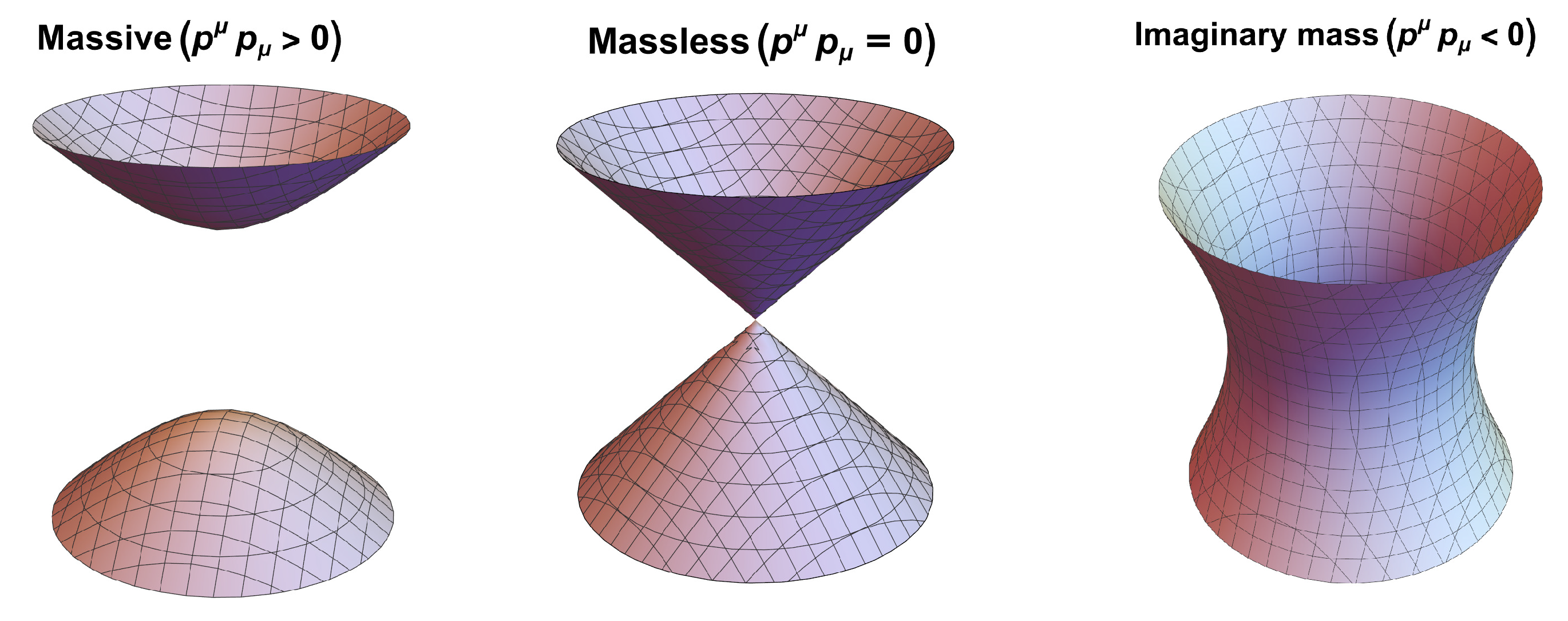
Figure 2.
The three parameters of the cylindrical group have physical interpretations. First, the top view accounts for the rotational degree of freedom and corresponds to the helicity of the photon. Then, the side view depicts up and down translations on the z-axis where they represent the gauge degrees of freedom [23].
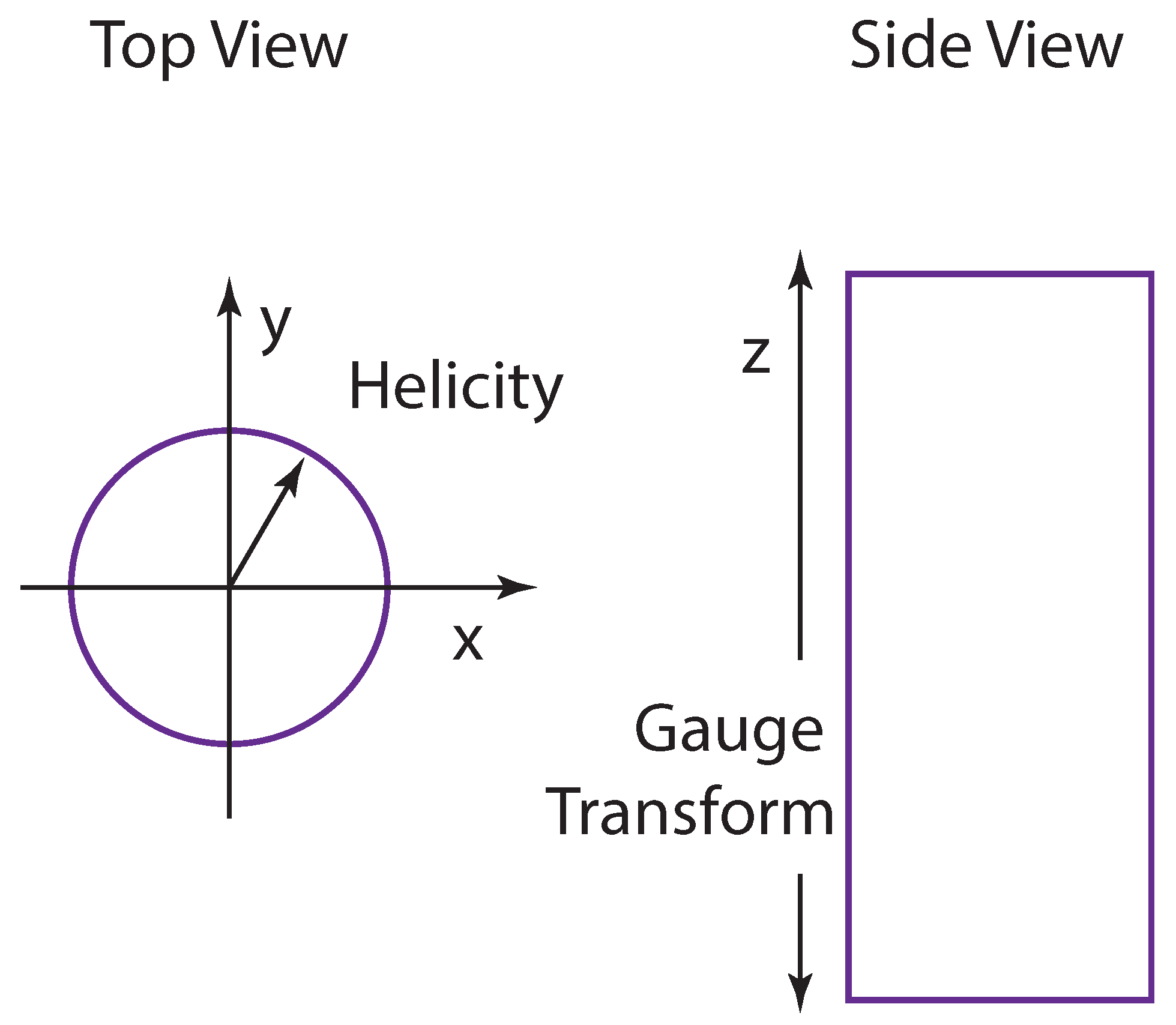
Figure 3.
Since Lorentz-squeezed momentum-energy and space-time wave functions have the same deformation properties, as the speed of the hadron approaches to that of light, both of these wave functions, as can be seen, become concentrated along positive light-cone axes, respectively. The concentrations along the light-cone are what lead to Feynman’s parton picture [36,37]. As the external signal is moving in the opposite direction to that of the hadron, it travels along the negative light-cone axis. Thus, this signal has an interaction time with the bound state which is much shorter than the oscillation period of the quarks inside the hadron. Hence this effect is often known as Feynman’s time dilation [32,33,38,39].
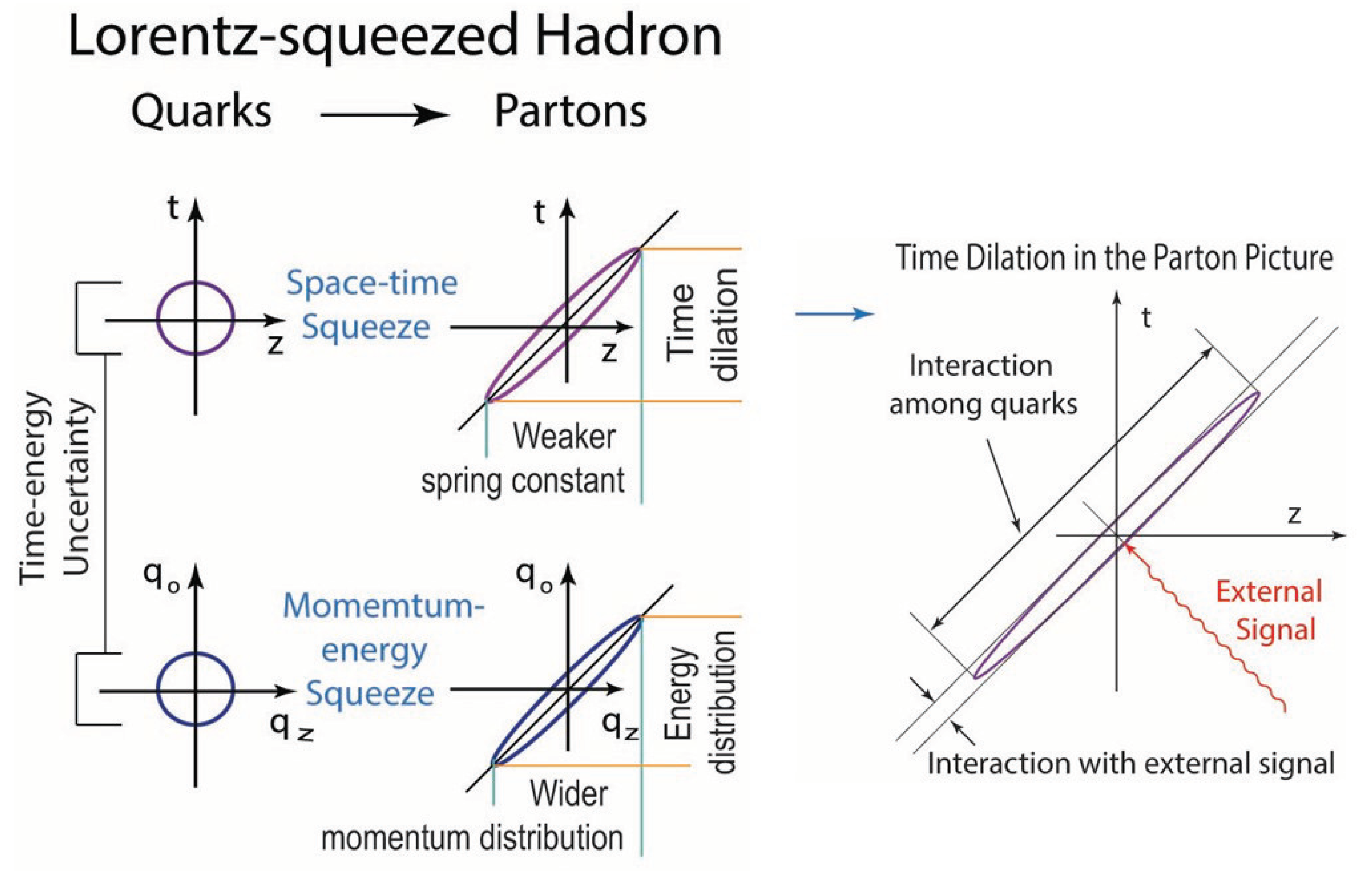
Figure 4.
The picture on left illustrates a resonator in a laser cavity. The light beam within the cavity is reflected back and forth for a very large number of times. The mathematical formulation is equivalent when the beam passes through a very large number of lenses. The figure on the right represents this analogous situation [45].
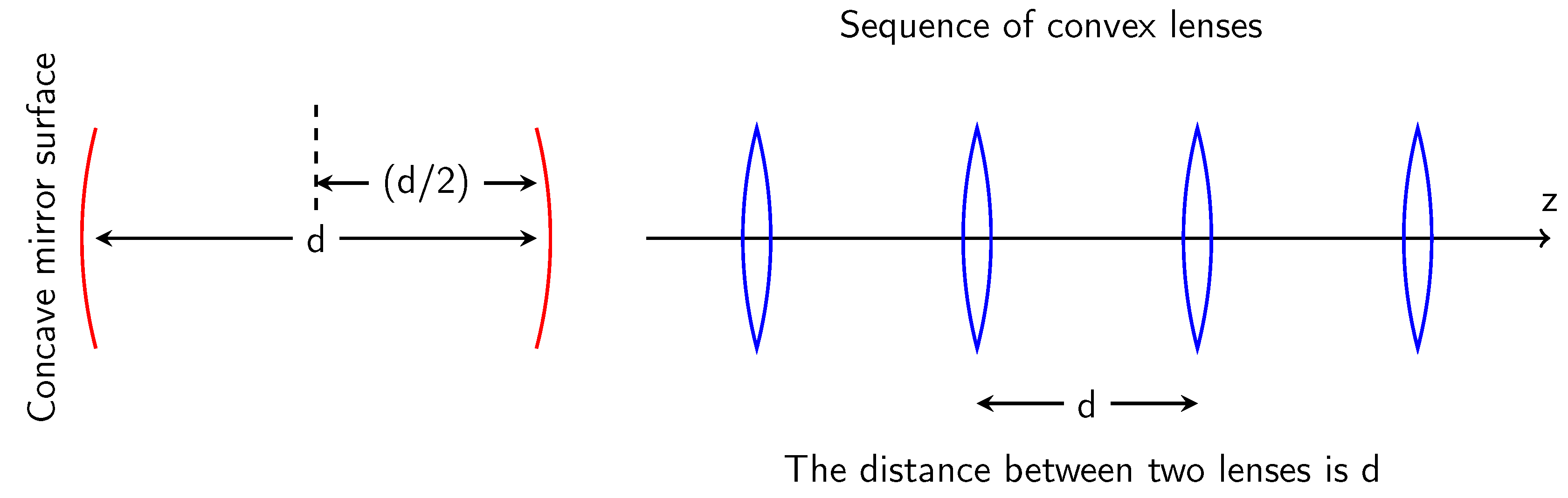
Table 1.
Four-momenta are represented by two-by-two matrices, labeled as , whose determinants are positive, zero, and negative for massive, massless, and imaginary-mass particles, respectively. remain invariant by their respective transformations. Therefore, matrices , belong to Wigner’s little group [15].
| Particle mass | Wigner four-vector | Wigner transformation matrix | ||
|---|---|---|---|---|
| Massive | ||||
| Massless | ||||
| Imaginary-mass |
Disclaimer/Publisher’s Note: The statements, opinions and data contained in all publications are solely those of the individual author(s) and contributor(s) and not of MDPI and/or the editor(s). MDPI and/or the editor(s) disclaim responsibility for any injury to people or property resulting from any ideas, methods, instructions or products referred to in the content. |
© 2025 by the authors. Licensee MDPI, Basel, Switzerland. This article is an open access article distributed under the terms and conditions of the Creative Commons Attribution (CC BY) license (http://creativecommons.org/licenses/by/4.0/).
Copyright: This open access article is published under a Creative Commons CC BY 4.0 license, which permit the free download, distribution, and reuse, provided that the author and preprint are cited in any reuse.


