
Submitted:
18 April 2025
Posted:
19 April 2025
You are already at the latest version
Abstract
Accurate prediction of gold prices is essential for informed financial decision-making, given their sensitivity to economic, political, and social factors. This study proposes a new hybrid framework for forecasting gold prices, combining traditional financial modelling, classical machine learning, and advanced deep learning methods, including long short-term memory networks and their variations. The framework integrates financial, macroeconomic, and sentiment indicators through feature fusion, capturing complex temporal dynamics and cross‑variable dependencies to improve prediction accuracy. The experimental evaluation spans a ten-year period (2014–2024), allowing for a robust assessment of framework performance in forecasting gold futures under varying market conditions. Comparative analysis of classical econometric and modern machine‑learning models shows that advanced methods achieve higher forecasting accuracy and remain robust despite data variability.
Keywords:
gold futures prediction
; financial time series
; deep learning
; machine learning
; macroeconomic indicators
; financial indicators
; sentiment analysis
; forecasting accuracy
1. Introduction
Gold remains a strategic asset in global finance, valued for its role as both a store of value and a hedge against inflation, currency risk, and geopolitical uncertainty (Reboredo, 2013). It is traded in various forms, including physical bullion, ETFs, and derivatives. Among these, gold futures stand out for their liquidity, standardization, and responsiveness to economic conditions, making them well-suited for predictive modelling. Gold futures contracts (GC=F), widely used as hedging instruments and safe-haven assets, have gained prominence due to their ability to mitigate price volatility and macroeconomic uncertainty (Fang et al., 2018). As they represent a growing share of global commodity trading (CME Group, 2025), interest in advanced forecasting methods – particularly deep learning (DL) – continues to rise in order to capture complex market dynamics and improve predictive accuracy.
The heightened volatility in gold prices has raised concerns about financial stability among policymakers, economists, and investors. Empirical studies confirm that gold price movements are closely linked to macroeconomic uncertainty, including inflation expectations, exchange rate fluctuations, and central bank interest rate policies (Beckmann et al., 2019). Understanding these drivers is thus essential for risk management, monetary policy development, and maintaining transparent financial systems.
Recent trends point to a growing global demand for gold (WGC, 2025), shifting global trade patterns, and more aggressive investment strategies seeking to hedge against financial volatility. Trading volumes in gold futures continue to expand, particularly in developed and emerging markets where inflation and geopolitical risk shape investor behaviour (Raza et al., 2018). In response, financial institutions are diversifying their product portfolios through leveraged gold instruments and digital trading platforms to appeal to risk-averse investors and sustain competitiveness (Gold Trading Platforms, 2025).
Despite the growing importance of accurately forecasting gold prices, there is still no unified framework that captures the full range of factors influencing gold price behaviour. Predicting gold price movements remains inherently complex for two main reasons:
- First, gold is affected by a wide array of interrelated influences – financial indicators, macroeconomic variables, and geopolitical events – creating a highly dynamic forecasting environment. Economic indicators such as the S&P 500, U.S. 10-year Treasury yields, and crude oil prices reflect investor sentiment, while geopolitical factors, including those measured by risk indices, can lead to sudden shifts in market behaviour (Baur & Smales, 2020). These variables often interact in non-linear and unpredictable ways, contributing to significant volatility and making it difficult to model gold prices within a single analytical structure.
- Second, the rise of high-frequency data and sentiment-driven variables requires more advanced prediction methods. Traditional statistical models like ARIMA and GARCH, along with basic machine learning (ML) approaches (Adebiyi et al., 2014), offer useful insights but often fail to capture complex, non-linear patterns. With the growth of financial technologies, it is now possible to monitor economic and political sentiment in real time, greatly expanding the available data. This shift has increased interest in DL techniques, especially long short-term memory (LSTM) networks (Fischer & Krauss, 2018), which are effective in modelling time-dependent data and uncovering hidden relationships among input variables.
These challenges motivate the development of a unified framework that integrates multiple financial indicators, macroeconomic variables, and sentiment-based measures for improved gold price prediction. By combining traditional econometric methods with advanced ML and DL techniques, the study aims to capture both linear and non-linear relationships that drive gold price behaviour under diverse market conditions. Specifically, the incorporation of DL architectures enhances the model’s ability to uncover complex temporal and cross-variable patterns.
To achieve this goal, the study first proposes a new conceptual framework that systematically examines how financial, macroeconomic, and sentiment factors interact to influence gold price. A dataset for gold futures spanning the period from 2014 to 2024 is collected, incorporating relevant economic indicators, commodity prices, and sentiment indices. Then, the most influential variables are identified and assessed for their contribution to forecasting accuracy. Multiple predictive models – including traditional statistical methods and advanced supervised learning approaches – are then constructed, tested, and compared to evaluate their robustness and forecasting performance of gold futures across varying economic regimes.
This new integrated approach not only validates the predictive value of combining classical and modern techniques but also offers practical insights for investors, financial institutions, and policymakers seeking resilient strategies in the face of growing market uncertainty and complexity.
The remainder of this paper is organized as follows. Section 2 reviews current literature on gold price prediction, emphasizing the economic, financial, and sentiment-based factors of gold price fluctuations. In Section 3, the focus shifts to the design of the proposed methodological framework, describing data collection, chosen indicators, and applied prediction methods. Section 4 addresses model construction and validation, comparing their performance with forecasting models from similar previous studies. Finally, Section 5 summarizes the core findings, acknowledges the study’s limitations, and suggests directions for future research.
2. Related Work
In this section, we review recent studies on gold price forecasting with emphasis on both the types of data used and the modelling techniques applied. The analysis compares key aspects such as target variables, input features, modelling approaches, and evaluation metrics, highlighting current trends and best practices that support the development of data-driven and interpretable gold price forecasting frameworks.
Hajek and Novotny (Hajek and Novotny, 2022) presented an interpretable approach to gold price forecasting using a fuzzy rule-based system that combines financial variables with news sentiment indicators. Their results underscore the importance of sentiment factors for short-term (one-day-ahead) predictions, while traditional financial indicators remain effective for longer horizons. The proposed hybrid model delivers both high predictive accuracy and interpretability, offering rule-based insights into the dynamics of gold prices.
Liang et al. (Liang et al., 2022) proposed a new hybrid forecasting framework—ICEEMDAN-LSTM-CNN-CBAM (ILCC)—for gold price prediction by integrating signal decomposition with DL techniques. The model begins with Improved Complete Ensemble Empirical Mode Decomposition with Adaptive Noise (ICEEMDAN) to decompose the time series into Intrinsic Mode Functions (IMFs). These components are then processed through a DL architecture that combines LSTM networks, Convolutional Neural Networks (CNN), and a Convolutional Block Attention Module (CBAM). The study demonstrated that the proposed ILCC framework significantly outperformed both conventional and hybrid models in predictive accuracy, as confirmed by the Model Confidence Set (MCS) test.
Mousapour Mamoudan et al. (Mousapour Mamoudan et al., 2023) developed a hybrid DL framework that combines CNN and Bidirectional Gated Recurrent Units (BiGRU), optimized using metaheuristic algorithms such as the Firefly Algorithm (FA) and Moth-Flame Optimization (MFO), to enhance signal accuracy in the gold market. The model was trained on 112 technical indicator-based features extracted from 10 months of gold market data. The results demonstrated the effectiveness of integrating neural networks with metaheuristics for robust classification and prediction in highly volatile commodity markets.
Stanković et al. (Stanković et al., 2023) introduced a new DL-based framework for univariate gold price forecasting using a Bi-directional LSTM (BiLSTM) network. The study introduces an improved Teaching-Learning Based Optimization algorithm (ITLB) to optimize BiLSTM hyperparameters, combined with Variational Mode Decomposition (VMD) to extract meaningful trends from the raw gold price data. The model was tested on daily gold prices from 2020 to 2022 and benchmarked against other metaheuristic algorithms. The proposed VMD-BiLSTM-ITLB approach achieved superior performance, demonstrating its robustness and forecasting accuracy in multi-step gold price prediction tasks.
Amini and Kalantari (Amini & Kalantari, 2024) designed a hybrid DL framework for predicting gold prices using CNN and BiLSTM models. The authors also highlight the effectiveness of combining spatial feature extraction (CNN) and temporal modelling (Bi-LSTM) in capturing complex nonlinear patterns in gold price dynamics.
Gür (Gür, 2024) investigated the predictive performance of DL architectures on gold price movements, incorporating macroeconomic variables and market sentiment data. The study proposes a hybrid model combining CNN, LSTM and GRU to enhance temporal feature extraction and improve interpretability. The dataset includes daily gold prices between 2017 and 2023. The study emphasizes the potential of attention-based neural networks for financial time series forecasting.
Pokou et al. (Pokou et al., 2024) developed a hybrid DL framework that combines Bi-directional LSTM and attention mechanisms for predicting gold prices. The study addresses the limitations of traditional time series models by incorporating temporal dependencies and relevant feature attention into the forecasting process. Using daily gold price data from 2012 to 2022, the proposed model is benchmarked against standard LSTM, GRU, and ML models. The results demonstrate that the BiLSTM with attention mechanism significantly improves prediction accuracy compared to baseline models.
Qiu et al. (Qiu et al., 2024) built a two-stage hybrid DL framework for gold price forecasting. It first uses VMD to cluster time series data, then refines predictions via aresidual correction stage using backpropagation (BP), LSTM, and CNN models. This approach improves accuracy of gold futures price prediction across four major gold markets, addressing the limitations of single-model methods.
Tashakkori et al. (Tashakkori et al., 2024) proposed a new model based on Multi-layer Perceptron (MLP) neural networks for forecasting gold prices using gold trading data, specifically the Open, High, Low, Close prices, and trading Volume (OHLCV) as input features. Unlike DL hybrids, the study focuses on assessing the standalone performance of an optimized MLP architecture using historical gold price data. The results demonstrated that the proposed MLP-based method delivers competitive accuracy, highlighting its potential as a lightweight and efficient alternative for financial time series prediction.
In their study (Zangana and Obeyd, 2024), Zangana and Obeyd created a DL-based system for gold price forecasting using historical time series data. The authors employ LSTM and BiLSTM models to capture temporal dependencies and improve prediction accuracy. The model inputs include key economic indicators such as crude oil prices, exchange rates, inflation, and interest rates. The study also applied SHAP values to interpret feature importance, identifying crude oil and USD/EUR as major contributors to prediction performance.
Table 1 summarizes key models for gold price prediction, outlining modeling approaches, data sources, and variables examined. The analysis shows that recent studies on gold price prediction can be classified based on several criteria, including research objectives, prediction methods, dataset characteristics, target variables, types of input data, modelling techniques, evaluation metrics, and overall model performance.
Based on the proposed methodologies, Hajek and Novotny, Mousapour Maroudan et al., Qiu et al., and Zandana and Obeyd introduced new multi-stage or hybrid forecasting frameworks aimed at improving predictive performance through techniques such as feature decomposition, feature fusion, and residual correction (Hajek & Novotny, 2022), (Mousapour Maroudan et al., 2023), (Qiu et al., 2024), (Zandana & Obeyd, 2024). In contrast, the rest of studies presented new predictive methods, including hybrid DL architectures (e.g., CNN-LSTM-GRU), DL models with automated parameter tuning, enhanced ARIMA (Pokou et al., 2024) and MLP-based (Tashakkori et al., 2024) models specifically designed for financial time series forecasting.
An additional classification dimension is the modelling approach. Most studies apply advanced DL architectures, frequently in hybrid combinations. CNN and BiLSTM structures dominate, as seen in Amini & Kalantari (2024) and Mousapour Mamoudan et al. (2023), with spatial and temporal features learned simultaneously. Liang et al. (2022), Stanković et al. (2023), and Qiu et al. (2024) combine decomposition and prediction into multi-stage pipelines. In contrast, Hajek & Novotny (2022) take an interpretable approach via fuzzy rule-based systems. Several works also use metaheuristic optimization techniques to tune model parameters: Firefly and Moth-Flame (Mousapour Mamoudan et al., 2023), Improved Teaching-Learning Based Optimization (Stanković et al., 2023), and the Whale Optimization Algorithm (Tashakkori et al., 2024), emphasizing an emerging trend in adaptive modelling.
Another way to classify the reviewed studies on gold price forecasting is by their modelling scope—specifically, whether they employ a univariate or multivariate approach. Several studies adopted a univariate modelling strategy, relying solely on historical gold price data without incorporating external variables (Liang et al., 2022; Stanković et al., 2023; Amini & Kalantari, 2024; Gür, 2024; Pokou et al., 2024; Qiu et al., 2024). These models focus on capturing intrinsic temporal patterns and trends within the gold price series. The remaining studies followed a multivariate approach, integrating additional input features such as macroeconomic indicators, technical trading signals, or sentiment data. This broader scope enables a more comprehensive representation of the factors influencing gold price dynamics.
Another key way to classify the reviewed studies is by the type of dependent variable they aim to predict. While all focus on forecasting the value of gold, there are subtle differences in how the target variable is defined. Some studies concentrate on gold futures prices or spot prices, while others consider short-term versus long-term forecasting horizons. For instance, Liang et al. (2022) and Qiu et al. (2024) model gold futures, while Amini & Kalantari (2024) and Tashakkori et al. (2024) use daily historical price data. Although Gür (2024) centers on silver, the architecture is transferable to gold price prediction.
A further classification concerns the independent variables used in the forecasting models. These input features vary significantly across the studies, reflecting different assumptions about what influences gold price movements. Technical indicators like MACD, moving averages, and RSI are used in studies by Mousapour Mamoudan et al. (2023), Amini & Kalantari (2024), and Tashakkori et al. (2024). Meanwhile, Hajek & Novotny (2022) and Zangana & Obeyd (2024) adopt a broader scope by including macroeconomic variables and sentiment data, with Hajek & Novotny being the only study incorporating news sentiment analysis. Decomposition techniques such as ICEEMDAN and VMD are used by Liang et al. (2022), Stanković et al. (2023), and Qiu et al. (2024) to preprocess raw time series data, providing smoother signals for prediction.
Finally, the studies differ in the evaluation metrics they use to validate their models. MAE and RMSE are the most widely reported, used across nearly all studies. R² is also frequently employed to assess model fit, particularly in DL settings such as those in Stanković et al. (2023), Gür (2024), Qiu et al. (2024), and Zangana & Obeyd (2024). For classification tasks like that in Mousapour Mamoudan et al. (2023), metrics including accuracy, F1-score, and ROC-AUC are applied. Some studies incorporate additional dimensions of evaluation: Hajek & Novotny (2022) emphasize interpretability and economic performance (e.g., average annual return), while Liang et al. (2022) use the Model Confidence Set (MCS) to statistically validate the superiority of their hybrid model.
The analysis confirms that most researchers rely on only one or two main types of modelling approaches – statistical, ML, or DL. Among these, LSTM-based architectures are particularly favoured for financial time series forecasting due to their ability to capture long-term dependencies and complex non-linear patterns. Only one recent study incorporates two key groups of external factors – macroeconomic indicators and sentiment-related variables such as news sentiment – to enhance prediction accuracy. Despite these advancements, the literature still lacks a unified framework that systematically combines diverse external variables with advanced data analysis techniques for gold price forecasting. To address this gap, the following section introduces a novel methodology that leverages the strengths of traditional and modern forecasting methods and integrates a broad set of financial, macroeconomic, and sentiment-based features to improve the predictive performance of gold price models.
3. A New Methodology for Gold Price Prediction Using Fusion of Financial, Macroeconomic, and Sentiment Data
The next subsection will describe the structure and rationale of your gold price prediction framework, highlighting how financial, macroeconomic, and sentiment indicators are integrated for improved forecasting performance.
3.1. Conceptual Framework for Gold Price Forecasting via Various Input Factors
This section details the methodological framework designed for gold price prediction, incorporating three categories of input variables – financial, macroeconomic, and sentiment indicators – and combining three modelling approaches: classical statistical techniques, ML algorithms, and advanced DL architectures. The goal is to harness the strengths of each method while fully capturing the multifaceted drivers of gold price movements. Figure 1 shows the flowchart of proposed new hybrid methodology.
Below is a step-by-step outline of the proposed methodology for data analysis, beginning with data collection and finishing in results interpretation and stakeholder recommendations:
1. Data Collection and Integration
The process begins with data collection and integration, where relevant financial indicators, macroeconomic variables, and sentiment measures are gathered from reputable databases. These datasets must then be synchronized to a common temporal frequency, such as daily or weekly intervals, ensuring consistency across all variables. Once aligned, the data is consolidated into a single dataset that will serve as the foundation for subsequent modelling steps.
2. Data Preprocessing
Following data collection, preprocessing is necessary to clean and validate the dataset. Missing values are handled through imputation or removal, while outliers are detected and addressed to maintain data integrity. Numerical features undergo normalization using min-max scaling or standardization, whereas categorical or sentiment-based inputs are processed through label encoding or numerical conversion. Feature engineering is also applied, constructing additional variables such as lag features or rolling averages that capture temporal dynamics and interactions among financial, macroeconomic, and sentiment indicators.
3. Model Selection and its Configuration and Setup
The next phase involves model selection, configuration, and parameter setup. For ML and DL methods, the dataset is partitioned into training and testing subsets. Error metrics, including mean squared error, mean absolute error, and financial-specific measures such as directional accuracy, are defined to evaluate performance. Each modelling approach is then configured with its respective parameters, ensuring that both classical and advanced techniques are appropriately tuned. For DL methods, hyperparameters such as the number of layers and dropout rates are fine-tuned using validation data.
To assess the predictive performance of various methods for gold price forecasting, we applied different modelling techniques categorized into three major groups: classical financial models, ML methods, and DL architectures. These model types were selected to capture diverse data characteristics – linear and nonlinear patterns, seasonal effects, and complex temporal dependencies.
The combination of diverse methods and complementary metrics ensures a reliable and comprehensive assessment framework. This allows us to evaluate model robustness, generalization capability, and practical applicability across different forecasting scenarios.
4. Comparative Analysis
Once the models are trained and optimized, a comparative analysis is conducted to evaluate their performance across different methodologies. Error metrics are used to compare the predictive accuracy of statistical, ML, and DL models. Robustness checks are performed by assessing model stability during periods of market volatility or external shocks, such as geopolitical events.
5. Interpretation of Results
The interpretation of results is crucial for identifying the most influential predictors. Statistical significance tests highlight the impact of financial, macroeconomic, and sentiment indicators on the final predictions. To better understand the output of the ML and DL models used in this framework, model-agnostic interpretability tools were employed. LIME (Local Interpretable Model-agnostic Explanations) (Ribeiro et al., 2016) and SHAP (SHapley Additive exPlanations) (Lundberg & Lee, 2017) can be utilised because they provide transparent, consistent, and intuitive explanations of black-box model predictions – an important consideration in financial contexts where interpretability and trustworthiness are essential (Ribeiro et al., 2016; Lundberg & Lee, 2017).
6. Stakeholder Recommendations
Finally, stakeholder recommendations are developed based on the findings. Investors and financial institutions are advised on the most effective predictive methods and indicator subsets for optimizing portfolio strategies or hedging tactics. Policy and regulatory bodies receive insights into how macroeconomic and sentiment indicators might inform monetary policies and economic stability measures.
In summary, this framework ensures a structured workflow, from initial gold price data acquisition to final recommendations, leveraging a combination of classical, ML, and DL models to yield comprehensive insights into gold price dynamics. This methodology systematically integrates financial, macroeconomic, and sentiment data with three tiers of predictive models – statistical, ML, and DL – to provide a holistic framework for accurate and resilient gold price forecasting.
3.2. Most Widely Used Methods in Gold Price Forecasting
This section outlines the key preprocessing and prediction methods commonly used for gold price data preparation and modelling, along with model tuning details.
In preprocessing stage, we employ a variety of statistical and econometric techniques:
- Correlation analysis assesses the linear relationships between gold and other financial and macroeconomic variables, including silver, platinum, bond yields, stock indices, and inflation indicators.
- Cross-correlation analysis explores lead-lag relationships between gold and time-sensitive variables such as oil prices, monetary policy rates, and global economic uncertainty.
- Variance Inflation Factor (VIF) (O'Brien, 2007) diagnostics detect and address multicollinearity, allowing us to remove or consolidate highly correlated variables to prevent distortion in regression-based models.
- Markov regime-switching models (Hamilton, 1989) capture different volatility regimes in the gold market, helping to distinguish between periods of stability and crisis.
- Linear and polynomial regression techniques test the statistical significance and potential nonlinear effects of selected predictors.
- Ridge regression identifies key explanatory variables while minimizing the impact of multicollinearity, thereby improving model stability.
- Cluster analysis classifies historical gold price patterns into distinct behavioural regimes, offering additional insights into market structure.
- Wavelet analysis examines long-term and cyclical co-movements between gold and input indicators.
Together, these methods enable us to isolate the most influential and reliable predictors of gold price dynamics under varying economic conditions, while systematically excluding irrelevant or redundant variables from the modelling process.
Some of the most widely used classical and advanced financial models for gold price prediction are:
- SARIMAX (Seasonal AutoRegressive Integrated Moving Average with eXogenous variables) is a time-series model that can capture trend, seasonality, and the influence of external factors in a structured, interpretable form:
- Prophet (Taylor & Letham, 2018), is an additive model designed to handle seasonality, holidays, and missing data with minimal tuning, making it especially useful for business-oriented time series with regular cycles. Prophet is a statistical model with –ML-friendly usability that lies between traditional time series methods and modern ML techniques. It does not require large datasets or GPU resources, making it well-suited for fast, interpretable forecasting using limited data and minimal computational effort. The model decomposes a time series into trend, seasonality, and holiday components as follows:
The ML methods include:
- Stochastic Gradient Descent (SGD) for regression is an iterative optimization algorithm that updates model parameters using the gradient of the loss function computed on a single or small batch of training examples to minimize prediction error efficiently (Bottou, 2010). Its update rule formula is:
- Support Vector Regression (SVR) (Smola & Schölkopf, 2004) , effective for high-dimensional regression problems. It uses kernel functions to model complex relationships and is robust to overfitting. SVR tries to find a function that deviates from the actual targets by at most ε:
- Random Forest (RF) (Breiman, 2001), a tree-based ensemble method that improves prediction accuracy through bootstrapping and aggregation, while also offering feature importance insights:
The DL models adopted are:
- GRU (Gated Recurrent Unit) (Cho et al., 2014) is a lightweight recurrent neural network architecture that captures sequential patterns while requiring fewer parameters than traditional RNNs:
- LSTM (Long Short-Term Memory) networks are Recurrent Neural Networks (RNNs) capable of learning long-term dependencies in sequence data (Hochreiter & Schmidhuber, 1997). They address vanishing gradient issues using gating mechanisms. At each time step t:
Where is forget gate vector, – input gate vector, – candidate cell state, – updated cell state, – cell state from the previous time step, – output gate vector, , , , – weight matrices, , , , – bias vectors. Final prediction is:
- Bi-LSTM (Bidirectional LSTM) (Graves & Schmidhuber, 2005) is an extension of LSTM that processes the input sequence in both forward and backward directions, enhancing context comprehension:
- CNN (Convolutional Neural Network) (LeCun et al., 2015) detect local patterns and structural changes in time series data through convolutional filters.
- ConvLSTM (Shi et al., 2015) is a hybrid model that combines the spatial feature extraction of CNN with the temporal modelling capabilities of LSTM, making it particularly effective for spatio-temporal data.
Although gold prices do not exhibit strong seasonal patterns, SARIMAX was employed for its flexibility to include exogenous variables and model temporal dependencies. In our case, the model functions as an ARIMAX by capturing trend and lagged effects of both the target and explanatory variables without relying on seasonality. Classical and hybrid models such as SARIMAX and Prophet respectively are transparent and easy to interpret, but they may struggle with nonlinear or irregular patterns. ML models like RF and SVR handle complex relationships better, though they require careful tuning and often lack interpretability. SGD-based regression was chosen for its efficiency and scalability in training linear models on time series data, offering a fast and adaptive ML approach suitable for high-frequency and volatile financial datasets such as gold prices. DL models offer the highest flexibility and accuracy, particularly for capturing long-term dependencies and interactions among multiple factors. However, they demand more data, computational resources, and expertise.
To optimize model performance and prevent underfitting or overfitting, each forecasting algorithm should undergo a systematic hyperparameter tuning process. For classical models such as SARIMAX and Prophet, parameters related to trend, seasonality, and external regressors are selected based on information criteria (e.g., AIC, BIC) and visual inspection of residual diagnostics. For ML models, hyperparameters are fine-tuned using a grid search approach in combination with time series cross-validation. Key parameters such as kernel type and regularization strength (for SVR), number of estimators and maximum depth (for RF), and learning rate and penalty function (for SGD) are varied within predefined ranges to identify configurations that minimize prediction error. For DL models, a combination of manual tuning and automated random search is applied. Critical hyperparameters include the number of hidden units, number of layers, dropout rate, activation functions, batch size, and number of epochs. Early stopping is employed to halt training when validation loss stops improving, thereby reducing the risk of overfitting.
3.3. Most Widely Used Metrics for Performance Evaluation
To evaluate the performance of forecasting models, can be used four widely accepted regression metrics:
Mean Absolute Error (MAE) measures the average magnitude of errors in predictions without considering their direction. It is simple to compute and provides an intuitive understanding of model accuracy.
Mean Squared Error (MSE) calculates the average of the squared differences between predicted and actual values, placing greater weight on larger errors. It is useful when large errors are particularly undesirable.
Root Mean Squared Error (RMSE) represents the square root of the MSE, retaining the unit of the target variable and offering better interpretability while still penalising large errors.
Coefficient of Determination (R²) indicates the proportion of variance in the dependent variable that is predictable from the independent variables. It provides a relative measure of model performance compared to a simple mean-based prediction.
This list can be expanded with additional metrics depending on the method group used. For classical statistical models, metrics such as Akaike Information Criterion (AIC) and Bayesian Information Criterion (BIC) are often applied. For ML models, metrics like Mean Bias Deviation (MBD) and Median Absolute Error may offer further insight. In the context of DL approaches, more advanced metrics such as sMAPE and Explained Variance Score are also commonly employed to assess model robustness and generalization.
Using standard performance metrics such as MAE, MSE, RMSE, and R², the proposed multi-stage tuning procedure ensures that each model is optimized for both accuracy and generalizability under diverse market conditions.
The proposed theoretical framework enhances predictive performance while providing a robust tool for interpreting the dynamic factors that influence gold prices.
4. Experimental Results
This section evaluates the effectiveness of the proposed framework through empirical testing of the developed models and a comparison of their performance across different market environments.
1. Data Collection and Integration
The selection of independent variables for gold futures price prediction was grounded in both economic theory and empirical evidence, incorporating financial market dynamics, macroeconomic fundamentals, and sentiment-based influences. A total of 19 candidate predictors were initially identified, reflecting three key domains – ten financial market indicators, seven macroeconomic variables and two sentiment indices. Table A1 presents the list of indicator abbreviations, their full names and descriptions.
From the financial view point, the model includes leading indicators such as continuous commodity futures (for Copper, Crude Oil, Palladium, Platinum, and Silver), benchmark stock indices (MSCI World ETF, NASDAQ, S&P 500), the yield on 10-year U.S. Treasury bonds, and the Volatility Index (VIX). These indicators reflect investor expectations, global risk levels, market sentiment, and the relationship between gold and other strategic assets.
The selection of specific variables was guided by their economic relevance and theoretical connection to gold market dynamics. For example, Copper Futures (HG=F) are widely used in the industry and are closely linked to overall economic activity, which makes them a useful proxy for economic growth expectations. Since changes in copper prices often signal upcoming shifts in the economy, they can also influence demand for gold as an alternative asset. Crude Oil Futures (CL=F) are another critical variable, as rising oil prices contribute to higher production costs and inflation, both of which may increase investor interest in gold as a hedge. Palladium (PA=F) and Platinum (PL=F) are two precious metals that are often associated with gold, and fluctuations in their prices can reflect changing sentiment in the broader precious metals market. Silver Futures (SI=F) typically move in correlation with gold and therefore offer additional insight into market trends. Regarding stock indices, we included the MSCI World ETF because it tracks equities from developed economies and serves as a global market benchmark. The NASDAQ index reflects the technology sector and is sensitive to innovation and risk tolerance; in times of uncertainty, gold is often seen as a safer investment. The S&P 500 is a key benchmark for the U.S. market, and shifts in this index can signal changes in capital flows, which tend to influence gold prices. The 10-year U.S. Treasury yield indicates investor expectations around inflation and monetary policy, and when yields rise, gold can become less attractive due to its non-yielding nature. The inclusion of the VIX is based on its ability to measure market uncertainty and investor fear; when the VIX is high, demand for gold often increases. These financial variables were retrieved from the website www.investing.com.
Given the leading role of the U.S. in the global economy and the fact that gold is primarily traded in U.S. dollars, our dataset focuses on seven U.S. macroeconomic indicators related to inflation, labour markets, interest rates, public debt, and economic growth. In this group, we included the Consumer Price Index (CPALTT01USM657N), which tracks inflation and reflects the purchasing power of consumers. Since gold is traditionally used as an inflation hedge, this indicator is crucial. The Federal Funds Rate (FEDFUNDS), set by the U.S. Federal Reserve, directly influences the attractiveness of alternative assets like gold. We also selected three labour market indicators – EMRATIO (Employment-Population Ratio), CIVPART (Labour Force Participation Rate) and UNRATE (Unemployment Rate) – as they provide insight into overall economic strength. When economic performance weakens, gold tends to become more attractive. Additionally, we included PSAVERT (Personal Savings Rate), which shows household saving behaviour. High levels of savings may reflect economic uncertainty and drive investors toward safer assets like gold. The final macroeconomic variable, GFDEGDQ188S (Federal Debt to GDP Ratio), measures fiscal sustainability, and high national debt can erode trust in the currency, increasing demand for gold. These official economic statistics were collected from the Federal Reserve Economic Data (FRED) and the World Bank online databases.
To further strengthen the model, we added two sentiment-based indicators. The Global Economic Policy Uncertainty Index (GEPUCURRENT) captures uncertainty in global economic policy and has a direct influence on investor behaviour, while the daily Geopolitical Risk Index (GPRD) reflects international tension and conflict, which often drives gold demand upward during crises. These sentiment indicators were sourced from PolicyUncertainty.com (Baker et al., 2025) and the Geopolitical Risk Index database by Caldara and Iacoviello (Caldara & Iacoviello, 2022).
To ensure consistency across all data sources, all variables were converted to a daily frequency using linear interpolation in case of macroeconomic factors. This allows full synchronization of the dataset, ensuring accuracy and coherence during the modelling process.
2. Data Preprocessing
Following the preprocessing (data cleaning, correlation analysis, multicollinearity diagnostics using VIF scores, and feature importance ranking using ML techniques), a refined set of independent variables was selected.
The analysis of descriptive statistics (Table A2) indicates that most financial variables are reasonably distributed, while certain metals and volatility indices exhibit heavy-tailed behaviour. Macroeconomic and sentiment indicators display structural asymmetries and periodic spikes, suggesting their suitability for regime-switching or interaction-based modelling. VIX shows pronounced non-normality, highlighting the need for careful preprocessing.
We also performed Pearson correlation analysis to evaluate the linear relationship between gold futures prices and a set of potential explanatory variables. This allowed us to identify those predictors with meaningful associations to gold, and to eliminate variables with limited or contradictory statistical significance. Based on a threshold of ±0.05, PSAVERT (Personal Savings Rate) and UNRATE (Unemployment Rate) were excluded from the initial dataset due to their negligible linear relationship with gold prices, as indicated by their correlation coefficients of 0.04 and –0.05, respectively. The results also indicate that silver exhibits a very strong positive correlation with gold (0.90), as shown in Table A3. As both are precious metals influenced by similar macroeconomic and geopolitical factors, their price movements tend to align closely. This well-established co-movement supports the inclusion of silver as a reliable predictor in our gold forecasting models, both statistically and economically. In contrast, platinum shows a very weak and negative correlation with gold (–0.12), providing no statistical basis for its inclusion. Palladium, although moderately correlated (0.47), is predominantly driven by industrial demand and is therefore less aligned with the investment-related dynamics that influence gold prices. Among these metals, silver stands out as the most appropriate proxy, combining strong statistical association with clear economic relevance to gold market behaviour. On the other hand, copper (0.78) primarily reflects industrial cycles, making it less relevant to the investment-driven dynamics of gold. Its inclusion is potentially redundant due to silver’s stronger correlation and comparable commodity characteristics. The three stock indices (MSCI World ETF, NASDAQ, and S&P 500), despite their high correlation coefficients (0.92, 0.93 and 0.94 respectively), were excluded due to their theoretical inconsistency, potential multicollinearity, and overlapping information content. With a correlation of 0.25, VIX shows limited standalone explanatory power for gold price dynamics. Additionally, Granger Causality test shows that stock indices and VIX do not directly predict gold price movements and should be omitted. CIVPART (Civilian Labour Force Participation Rate) shows moderate correlation (–0.42) but limited variability and responsiveness, reducing its forecasting utility. CPALTT01USM657N (Consumer Price Index, monthly % change) (0.49) captures short-term fluctuations with low standalone interpretability and is outperformed by more robust inflation and uncertainty indicators. GFDEGDQ188S (Federal Debt-to-GDP Ratio) is a low-frequency, structural indicator that reflects long-term fiscal trends but lacks responsiveness to short-term gold price movements. Its quarterly updates are misaligned with higher-frequency gold data, and its inflationary implications are already captured by more timely variables, making it redundant and potentially problematic for model stability.
Crude oil is included in the model due to its role as a key inflation proxy and macroeconomic indicator; its price movements often reflect global economic conditions and geopolitical tensions, both of which influence gold demand. The U.S. 10-year Treasury yield is also retained, as it represents the benchmark interest rate and reflects investor expectations for inflation and monetary policy—factors that affect the opportunity cost of holding gold. Although it shows a moderate positive correlation with gold, its economic relationship is typically inverse, making it a valuable explanatory variable. The employment-to-population ratio (EMRATIO) is preserved for its ability to capture overall labour market health more effectively than other employment metrics. A lower EMRATIO is often associated with increased demand for gold as a safe-haven asset during periods of economic uncertainty. Lastly, the federal funds rate (FEDFUNDS) is retained as a direct measure of monetary policy. It significantly influences real interest rates and investor behaviour, with rate increases generally leading to downward pressure on gold prices. Each of these variables contributes uniquely to understanding gold price movements and complements the broader macroeconomic and market sentiment context.
GEPUCURRENT (Global Economic Policy Uncertainty Index) is retained in the model due to its strong theoretical and empirical relevance to gold price movements. As a measure of global economic policy uncertainty, it captures shifts in investor sentiment that often drive demand for gold as a safe-haven asset. The variable demonstrates statistically significant relationships with gold in both linear and nonlinear analyses (Granger Causality test and Markov Switching Model) and complements other macroeconomic indicators by reflecting real-time market concerns that are not captured by structural data alone. Its inclusion enhances the model’s ability to predict gold price dynamics under varying economic and geopolitical conditions. To apply the Granger causality test and Markov switching model, we use Python (version 3.12.3) with the grangercausalitytests() and MarkovRegression() functions from the statsmodels library (version 0.14.4).
Although GPRD does not exhibit a strong correlation with gold (0.19), its inclusion is justified based on the results of the polynomial regression, which reveal a significant nonlinear relationship with gold prices. The analysis also shows that moderate increases in geopolitical risk tend to raise gold demand, aligning with gold's role as a safe-haven asset. However, the negative quadratic term suggests that when geopolitical uncertainty becomes extreme, this positive relationship weakens or may even reverse, indicating that investor behaviour can shift under conditions of severe crisis. These findings highlight that GPRD captures context-dependent effects not reflected in linear models and is particularly valuable for explaining gold price dynamics during periods of heightened geopolitical tension. Therefore, retaining GPRD enhances the model’s ability to reflect real-world investor responses under different market regimes.
The obtained final dataset consists of the following seven independent variables from the three factor groups: Crude Oil Futures (CL=F), Silver Futures (SI=F), US 10Y Treasury Yield; Employment-Population Ratio (EMRATIO), Federal Funds Rate (FEDFUNDS); Geopolitical Risk Index (GPRD), and Global Economic Policy Uncertainty Index (GEPUCURRENT). This subset was chosen based on their statistical significance, predictive power, and economic interpretability. These variables demonstrated lower multicollinearity, stable availability over the full analysis period, and strong theoretical links to gold price fluctuations. Their inclusion allows the model to capture a balanced spectrum of influences—ranging from monetary policy and labour dynamics to market volatility and geopolitical uncertainty—thus supporting more accurate and generalizable forecasting outcomes.
3. Model Selection and its Configuration and Setup
The SARIMAX model is configured with non-seasonal parameters (order = (0, 0, 0)) and disabled seasonal components (seasonal_order = (0, 0, 0, 12)), effectively reducing it to a regression model with exogenous variables—functionally equivalent to ARIMAX. This simplified configuration yielded the best empirical performance in the current experimental setup, likely due to the absence of strong seasonal patterns and the dominance of external macroeconomic factors. Nevertheless, the SARIMAX is retained in full within the modelling pipeline, as it allows for future extensions involving seasonal dynamics and autoregressive behaviour, which may become relevant with longer time series or additional training data. The SARIMAX model is implemented using the SARIMAX class from the statsmodels library (version 0.14.0).
The SGD model is developed using the SGDRegressor class from the scikit-learn library (version 1.3.2). It functions as a linear regression model optimized via stochastic gradient descent. In this configuration, the model minimizes the mean squared error loss (loss='squared_error'), equivalent to ordinary least squares regression solved through iterative updates. Parameter estimation is performed using randomly selected mini-batches from the training data, which allows for significantly faster convergence, particularly in high-dimensional or large-scale datasets. The initial learning rate is set via eta0, and adaptive scheduling mechanisms are used to refine it during training.
The Prophet model decomposes the gold price into components such as trend, seasonality, holiday effects, and user-defined external regressors. In this implementation, a changepoint prior scale of 0.1 (changepoint_prior_scale=0.1) is applied to control trend flexibility, balancing generalization with sensitivity to macroeconomic shifts. The model incorporates seven exogenous variables through the add_regressor() function and performs maximum a posteriori (MAP) optimization over the specified priors. Prophet uses automated changepoint detection and applies the L-BFGS algorithm for parameter estimation within a generalized additive model (GAM) framework. No holiday effects or multiplicative seasonality were included, and regressors were kept unscaled to preserve interpretability. The model is implemented via the Prophet class from the prophet library (version 1.1.4).
The GRU model uses a 64-unit recurrent layer followed by dense layers of 64 and 32 neurons. The standard LSTM model contains a single LSTM layer with 64 memory cells, again followed by two dense layers. The Bidirectional LSTM model includes a bidirectional recurrent layer with 64 hidden units (units=64), followed by two fully connected layers with 64 and 32 neurons, and a final output neuron for regression. The CNN model starts with a Conv1D layer (filters=64, kernel_size=3), followed by MaxPooling1D, flattening, and dense layers. The ConvLSTM model captures spatiotemporal patterns using a 2D convolutional recurrent layer with 64 filters (filters=64) and kernel size (1, 3), followed by flattening and dense layers.
All DL models were implemented using TensorFlow Keras version 2.15.0. The Bi-LSTM was constructed with Bidirectional and LSTM layers; the LSTM model used the LSTM layer; the CNN model included Conv1D, MaxPooling1D, and Dense layers; and the ConvLSTM model employed the ConvLSTM2D layer. Each model was trained for 100 epochs using a batch size of 16 and optimized using the Adam algorithm with mean squared error as the loss function.
Following the algorithm presented in our prediction framework, a combination of implemented models – including SARIMAX, SGD, Prophet, GRU, LSTM, Bi-LSTM, CNN, and ConvLSTM – is designed to predict gold prices by capturing a wide range of linear, nonlinear, and temporal dependencies in the data. This diverse model set allows for a thorough comparison of forecasting approaches.
4. Comparative Analysis
The forecasting results across three methodological groups – traditional econometric models, ML regressors, and DL architectures – reveal distinct patterns in their ability to model temporal dependencies (Figure 2) and in predictive performance of gold futures prices (Table 2).
The traditional econometric model, SARIMAX, delivers moderate performance with an MAE of 148.75, RMSE of 185.31, and R² of 0.577. Although it incorporates exogenous variables and captures linear trends, its limited capacity to model nonlinearities and structural breaks constrains its effectiveness. Nevertheless, SARIMAX outperforms several ML and DL models, underscoring its continued relevance when model interpretability is a priority.
In the ML category, the Stochastic Gradient Descent (SGD) regressor shows lower predictive accuracy (MAE = 190.96, RMSE = 229.21, R² = 0.353). While SGD is computationally efficient and well-suited to high-dimensional data, its linear formulation and sensitivity to hyperparameters reduce its effectiveness in modeling complex, nonlinear patterns typical of financial time series.
Among DL architectures, the Bi-LSTM model achieves the strongest performance (MAE = 113.65, RMSE = 145.60, R² = 0.739), outperforming the standard LSTM (MAE = 129.67, RMSE = 159.05, R² = 0.688) and GRU (MAE = 201.07, RMSE = 222.53, R² = 0.390). These results reflect the benefits of bidirectional processing in capturing both past and future dependencies. In contrast, convolutional models such as CNN (MAE = 181.30, RMSE = 227.17, R² = 0.364) and ConvLSTM (MAE = 199.03, RMSE = 227.23, R² = 0.364) underperform, likely due to their limited ability to model long-term sequential dependencies.
Surprisingly, the advanced forecasting model, Prophet, achieves the best overall performance (MAE = 76.30, RMSE = 102.34, R² = 0.871). Its strength lies in capturing structural trend changes and integrating external regressors, which are critical for modeling gold futures influenced by macroeconomic shocks. Unlike DL models that require large datasets and are prone to overfitting in volatile markets, Prophet handles irregularities and limited data more effectively through its additive structure and built-in changepoint detection.
In summary, the analysis confirms that Prophet and Bi-LSTM offer the highest forecasting accuracy. These models outperform traditional econometric and AI approaches, highlighting the importance of capturing nonlinearity, temporal memory, and structural dynamics—especially when using enriched input features such as macroeconomic indicators and sentiment signals.
5. Interpretation of Results
We now proceed to the next stage of our gold price prediction framework—results interpretation—with the aim of uncovering the influence of different input variables on model predictions. For this purpose, we focus on the BiLSTM model, which demonstrated the best overall performance among DL models in terms of predictive accuracy and temporal learning capacity. We apply SHAP to interpret the BiLSTM model (Figure 3), as SHAP is a widely accepted, model-agnostic technique that attributes each feature’s marginal contribution to the output, enabling both global and local insights.
The SHAP plot reveals that silver futures (SI=F) are the most impactful predictor of gold prices, with high values generally increasing predictions and low values reducing them. Other significant contributors include macroeconomic uncertainty indicators such as the Global Economic Policy Uncertainty Index (GEPUCURRENT) and the Geopolitical Risk Index (GPRD), reinforcing gold’s role as a safe-haven asset. Variables like crude oil prices, interest rates (US 10Y Treasury, FEDFUNDS), and employment ratio (EMRATIO) show moderate but context-sensitive effects. The coexistence of positive and negative SHAP values for single features illustrates the model’s ability to capture nonlinear and interaction-based dependencies common in financial markets.
While BiLSTM is interpreted through SHAP, other models in the framework also offer varying degrees of transparency. Prophet and SARIMAX provide built-in interpretability via trend decomposition and regression coefficients. For less interpretable models such as GRU, CNN, or ConvLSTM, SHAP or LIME can be used, albeit with higher computational demands. The final gold price prediction can be based on the best-performing model or synthesized through ensemble averaging, weighted by model performance metrics (e.g., MAE, RMSE), to enhance forecast robustness.
6. Stakeholder Recommendations
Based on the forecasting results and model interpretations, stakeholders in gold futures markets – such as investors, analysts, and policymakers – can be advised to prioritize models like Prophet and BiLSTM, which demonstrated superior accuracy and interpretability. The SHAP analysis identified silver futures, economic uncertainty (GEPUCURRENT), and geopolitical risk (GPRD) as the most influential predictors, suggesting that monitoring these indicators can improve decision-making. Investors and traders can leverage these models for dynamic portfolio adjustments, while policymakers may use the insights to anticipate the financial impact of macroeconomic and geopolitical developments. Ensemble forecasts combining linear and DL models are recommended for robust, context-sensitive predictions that account for both trend shifts and nonlinear dependencies.
5. Discussion
Our experimental results can be compared with those of similar previous studies using the following criteria: forecast accuracy, computational cost, interpretability, and methodological breadth. In terms of forecast accuracy, on our multivariate, daily-frequency gold-futures series, Prophet reaches R² = 0.871, MAE = 76.3, RMSE = 102.3, with Bi-LSTM close behind at R²= 0.739. Deep hybrid models from the literature achive even higher coefficients – Liang et al.’s ICEEMDAN-CNN-CBAM-LSTM reports R² ≈ 0.98 and Zangana & Obeyd’s Bi-LSTM R² = 0.95. However, these models rely on univariate or narrowly engineered inputs, whereas our Prophet model remains lightweight while using multivariate data. External-feature fusion also enables SARIMAX (R² =0.577) to surpass several neural networks, narrowing the historic gap between statistical and deep-learning models. Regarding evaluation metrics, Hajek &Novotny and Mousapour Mamoudan assess directional-classification tasks, reporting Accuracy, F1-score, and AUC rather than regression measures. This choice reflects that trading decisions often depend on up-versus-down moves, not precise price levels. Mmoreover, Mousapour Mamoudan et al.’s ten-month, highly volatile sample makes classification more stable than point forecasting. All other studies – including ours – predict continuous prices, so MAE, RMSE, and R² remain the appropriate performance metrics.
Performance metrics also vary across the compared studies. Hajek & Novotny and Mousapour Mamoudan report classification measures (Accuracy, F1, AUC) because their aim is directional trading and their short, volatile samples make class labels more reliable than point forecasts. The remaining studies—including ours—predict continuous prices, so regression metrics (MAE, RMSE, R²) are the appropriate choice.
The next comparison criterion is computational time. Prophet trains in seconds on a CPU, SARIMAX in minutes, and our Bi-LSTM (64 units, 100 epochs) converges in under 10 GPU-minutes. In contrast, Liang et al.’s triple-network pipeline and the Firefly-/Moth-Flame-optimised CNN-BiGRU of Mousapour Mamoudan demand far more GPU time and meta-heuristic tuning, making them impractical for daily retraining.
According to the next comparison criterion, interpretability, Prophet and SARIMAX reveal trend and coefficient effects directly; SHAP analysis of our Bi-LSTM highlights silver futures, GEPU and GPRD as key drivers. Only Hajek & Novotny’s fuzzy rules and Zangana & Obeyd’s SHAP plots offer comparable transparency, whereas most other hybrids sacrifice explainability in pursuit of lower error.
The studies compared cluster around four tactics – signal decomposition and deep networks, meta heuristic hyper parameter search, input fusion, and emerging post hoc explainers. We adopt the last two (financial-macroeconomic-sentiment fusion and explainability) while omitting costly decomposition and evolutionary tuning. As a result, Prophet and Bi LSTM offer top quartile predictive power at modest compute cost.
6. Conclusions
This study proposes a hybrid framework for predicting gold futures prices that: (1) fuses heterogeneous inputs – financial indicators, macroeconomic indices, and geopolitical/market-sentiment measures—into a single feature set and (2) blends multiple modelling techniques. Extensive preprocessing – correlation analysis, Granger causality, VIF screening, and regime-switching tests – removes redundancy and isolates the most influential variables, including Crude Oil, Silver futures, the US 10-year Treasury yield, the Employment-to-Population ratio (EMPRATIO), the Federal Funds Rate (FEDFUNDS), and sentiment indices such as GEPUCURRENT and GPRD. Polynomial regression further shows that political risk has a nonlinear impact on gold prices, underscoring the need for context-aware models that adapt to shifting regimes. The experimental results obtained with our fused-input framework confirm that Prophet and Bi-LSTM provide the highest accuracy and remain robust across varying market conditions.
Our framework offers several advantages: (1) it fuses heterogeneous inputs – financial, macroeconomic, and sentiment – into a single feature set; (2) it blends traditional and modern forecasting methods; and (3) it spans the full explainability spectrum, from instantly interpretable SARIMAX and business-friendly Prophet trend-seasonality to DL that expose nonlinear, regime-dependent patterns. By coupling every ML and DL model with SHAP and LIME, the framework retains transparency even for its deepest neural layers, enabling practitioners to see exactly how each variable shapes each forecast.
From a practical standpoint, this research offers valuable guidance for policymakers, investors, and financial analysts aiming to enhance gold-market forecasting and risk management. By identifying regime shifts, volatility clusters, and nonlinear drivers, it underscores the need for adaptive models that surpass traditional static approaches. These insights can support the development of hybrid trading algorithms, portfolio diversification strategies, and early-warning systems for market stress.
This study is not without limitations. First, the framework uses only historical data, omitting real-time sentiment and news texts that could add value. Second, while several models were tested, hyperparameter tuning was conducted in a standardized manner, leaving room for model-specific optimization. Third, shifting market relationships require regular model retraining and drift monitoring to maintain accuracy.
Future research should explore multimodal inputs – combining time series with real-time textual, social, and news data – and test transfer learning methods to enhance model generalization across time and regions. Additionally, extending the framework to comparative studies across different commodities and currencies could offer a broader understanding of interconnected financial systems. Refining prediction methods with advanced AI and richer datasets will help future studies foster more stable, responsive, and well-informed decision-making in commodity finance.
Author Contributions
Conceptualization, G.T.-A., S.R. and G.I.; methodology, G.T.-A. G.T.-A., S.R. and G.I.; software, G.T.-A., S.R., and G.I.; programming code, G.T.-A., and S.R.; validation, G.T.-A., S.R., and G.I.; investigation, G.T.-A.; resources, G.T.-A.; data curation, G.T.-A.; writing—original draft preparation, G.T.-A., S.R., and G.I.; writing—review and editing, G.T.-A., S.R., and G.I.; visualization, G.T.-A., S.R., and G.I.; supervision, G.I.; project administration, G.T.-A.; funding acquisition, G.I. All authors have read and agreed to the published version of the manuscript.
Funding
This research was partially funded the Ministry of Education and Science and by the National Science Fund, co-founded by the European Regional Development Fund, Grant No. BG05M2OP001-1.002-0002 and BG16RFPR002-1.014-0013-M001 “Digitization of the Economy in Big Data Environment”.
Informed Consent Statement
Not applicable.
Data Availability Statement
The dataset and Python code employed in this study are available from the authors upon request.
Acknowledgments
The authors thank the academic editor and anonymous reviewers for their insightful comments and suggestions.
Conflicts of Interest
The authors declare no conflicts of interest.
Appendix A
This appendix includes supplementary tables and figures that provide additional details on the dataset’s structure and temporal dynamics. These visualizations and summaries help clarify the behaviour of key indicators and their relevance to the gold price forecasting framework.

Table A1.
Gold futures and extended set of potential independent factors for their prediction.
| Abbreviation | Indicator Name | Description |
|---|---|---|
| GC=F | Gold Futures | A standardized contract to buy or sell gold at a predetermined price on a future date; widely used for hedging against inflation, managing risk, and speculating on gold price movements. |
| HG=F | Copper Futures | A contract to buy or sell copper at a future date, often viewed as an economic barometer. |
| CL=F | Crude Oil Futures | A standardized contract for buying or selling crude oil at a set price in the future. |
| MSCI | MSCI World ETF (Global Equity Fund) | An exchange-traded fund tracking a broad global equity index across developed markets. |
| NASDAQ | NASDAQ-100 | A global electronic marketplace listing many of the largest technology companies. |
| PA=F | Palladium Futures | A futures contract for palladium, a precious metal important in industrial applications. |
| PL=F | Platinum Futures | A futures contract for platinum, used as both an industrial metal and investment asset. |
| S&P 500 | S&P 500 | A market-capitalization-weighted index of 500 leading publicly traded companies in the US. |
| SI=F | Silver Futures | A contract to buy or sell silver at a future date, reflecting investors’ views on silver prices. |
| US 10Y Treasury | 10-Year US Treasury Bond Yield | The yield (interest rate) on the US government’s 10-year bond, a benchmark for global borrowing costs. |
| VIX | Volatility Index | A real-time market index indicating the market’s expectations of 30-day forward volatility. |
| CPALTT01USM657N | Consumer Price Index | Measures the weighted average of prices of a basket of consumer goods and services. |
| CIVPART | Civilian Labour Force Participation Rate | The percentage of the civilian population that is employed or actively seeking employment. |
| EMRATIO | Employment-Population Ratio | The proportion of a country’s working-age population that is employed. |
| FEDFUNDS | Federal Funds Rate | The interest rate at which depository institutions lend balances at the Federal Reserve to each other overnight. |
| GFDEGDQ188S | US Federal Debt to GDP Ratio | The ratio of total federal debt to the nation’s gross domestic product. |
| PSAVERT | US Personal Savings Rate | The proportion of disposable income that households save rather than spend. |
| UNRATE | Unemployment Rate | The percentage of the total labour force that is jobless and actively seeking employment. |
| GEPUCURRENT | Global Economic Policy Uncertainty Index | Captures the frequency of terms related to economic policy uncertainty across news sources worldwide. |
| GPRD | Geopolitical Risk Index | Measures the frequency of references to geopolitical tensions in major international newspapers. |
Table A2.
Descriptive statistics of the extended set of independent factors.
| Mean | Minimum | Maximum | St. Dev. | Skewness | Kurtosis | |
|---|---|---|---|---|---|---|
| Gold | 1564.84 | 1050.80 | 2788.50 | 377.82 | 0.83 | 0.02 |
| Copper | 3.21 | 1.94 | 5.12 | 0.74 | 0.41 | -0.93 |
| Crude Oil | 64.81 | 10.01 | 123.70 | 19.82 | 0.38 | -0.34 |
| MSCI World ETF | 97.76 | 61.22 | 161.14 | 24.89 | 0.60 | -0.76 |
| NASDAQ | 9283.92 | 3996.96 | 19486.79 | 4152.94 | 0.50 | -1.00 |
| Palladium | 1321.87 | 469.90 | 2985.40 | 636.74 | 0.73 | -0.68 |
| Platinum | 999.08 | 595.90 | 1516.00 | 160.17 | 1.37 | 1.75 |
| S&P 500 | 3207.00 | 1741.89 | 6032.38 | 1090.33 | 0.59 | -0.75 |
| Silver | 19.92 | 11.73 | 34.83 | 4.51 | 0.74 | -0.35 |
| US 10Y Treasury | 2.47 | 0.50 | 4.99 | 1.00 | 0.35 | -0.43 |
| VIX | 17.92 | 9.14 | 82.69 | 7.11 | 2.69 | 13.68 |
| CIVPART | 0.26 | -0.67 | 1.37 | 0.34 | 0.16 | 0.23 |
| CPALTT01USM657N | 62.55 | 60.10 | 63.30 | 0.53 | -1.42 | 2.03 |
| EMRATIO | 59.53 | 51.20 | 61.10 | 1.39 | -2.79 | 10.13 |
| FEDFUNDS | 1.62 | 0.05 | 5.33 | 1.84 | 1.03 | -0.38 |
| GFDEGDQ188S | 110.78 | 98.64 | 132.81 | 9.22 | 0.33 | -1.49 |
| PSAVERT | 6.80 | 2.00 | 32.00 | 4.05 | 2.95 | 10.20 |
| UNRATE | 4.81 | 3.40 | 14.80 | 1.66 | 2.91 | 11.10 |
| GEPUCURRENT | 211.33 | 86.89 | 431.79 | 70.33 | 0.25 | -0.52 |
| GPRD | 117.43 | 9.49 | 540.83 | 52.75 | 1.91 | 8.17 |
Table A3.
Correlation matrix.
| 1 | 2 | 3 | 4 | 5 | 6 | 7 | 8 | 9 | 10 | 11 | 12 | 13 | 14 | 15 | 16 | 17 | 18 | 19 | 20 | |
|---|---|---|---|---|---|---|---|---|---|---|---|---|---|---|---|---|---|---|---|---|
| Gold (1) | 1 | |||||||||||||||||||
| Copper (2) | 0.78 | 1 | ||||||||||||||||||
| Crude Oil (3) | 0.33 | 0.66 | 1 | |||||||||||||||||
| MSCI World ETF (4) | 0.92 | 0.87 | 0.41 | 1 | ||||||||||||||||
| NASDAQ (5) | 0.93 | 0.84 | 0.33 | 0.99 | 1 | |||||||||||||||
| Palladium (6) | 0.47 | 0.51 | 0.13 | 0.50 | 0.56 | 1 | ||||||||||||||
| Platinum (7) | -0.12 | 0.16 | 0.43 | -0.18 | -0.23 | -0.12 | 1 | |||||||||||||
| S&P 500 (8) | 0.94 | 0.84 | 0.38 | 1.00 | 0.99 | 0.50 | -0.24 | 1 | ||||||||||||
| Silver (9) | 0.90 | 0.82 | 0.41 | 0.83 | 0.83 | 0.44 | 0.22 | 0.82 | 1 | |||||||||||
| US 10Y Treasury (10) | 0.37 | 0.41 | 0.55 | 0.42 | 0.35 | -0.33 | -0.05 | 0.44 | 0.27 | 1 | ||||||||||
| VIX (11) | 0.25 | 0.07 | -0.11 | 0.10 | 0.19 | 0.49 | -0.26 | 0.15 | 0.08 | -0.27 | 1 | |||||||||
| CIVPART (12) | 0.49 | 0.61 | 0.33 | 0.54 | 0.52 | 0.31 | 0.10 | 0.52 | 0.54 | 0.14 | 0.00 | 1 | ||||||||
| CPALTT01USM657N (13) | -0.42 | -0.34 | 0.13 | -0.34 | -0.44 | -0.66 | 0.08 | -0.35 | -0.41 | 0.40 | -0.63 | -0.18 | 1 | |||||||
| EMRATIO (14) | -0.11 | 0.06 | 0.31 | 0.08 | -0.02 | -0.35 | -0.11 | 0.07 | -0.12 | 0.56 | -0.56 | 0.06 | 0.82 | 1 | ||||||
| FEDFUNDS (15) | 0.61 | 0.43 | 0.31 | 0.62 | 0.57 | -0.08 | -0.32 | 0.65 | 0.40 | 0.85 | -0.13 | 0.15 | 0.23 | 0.44 | 1 | |||||
| GFDEGDQ188S (16) | 0.85 | 0.62 | 0.11 | 0.78 | 0.84 | 0.71 | -0.26 | 0.80 | 0.71 | 0.04 | 0.54 | 0.35 | -0.75 | -0.44 | 0.34 | 1 | ||||
| PSAVERT (17) | 0.04 | -0.18 | -0.51 | -0.08 | 0.02 | 0.41 | -0.15 | -0.08 | -0.02 | -0.58 | 0.52 | -0.13 | -0.66 | -0.81 | -0.32 | 0.40 | 1 | |||
| UNRATE (18) | -0.05 | -0.26 | -0.36 | -0.27 | -0.19 | 0.15 | 0.17 | -0.27 | -0.05 | -0.57 | 0.45 | -0.17 | -0.62 | -0.96 | -0.49 | 0.24 | 0.79 | 1 | ||
| GEPUCURRENT (19) | 0.53 | 0.22 | -0.09 | 0.45 | 0.52 | 0.63 | -0.58 | 0.51 | 0.28 | -0.06 | 0.58 | 0.10 | -0.47 | -0.26 | 0.27 | 0.71 | 0.38 | 0.13 | 1 | |
| GPRD (20) | 0.19 | 0.24 | 0.31 | 0.21 | 0.18 | 0.00 | -0.02 | 0.22 | 0.16 | 0.31 | 0.01 | 0.21 | 0.11 | 0.24 | 0.22 | 0.07 | -0.31 | -0.27 | 0.05 | 1 |
Figure A1.
Historical prices of Gold futures.
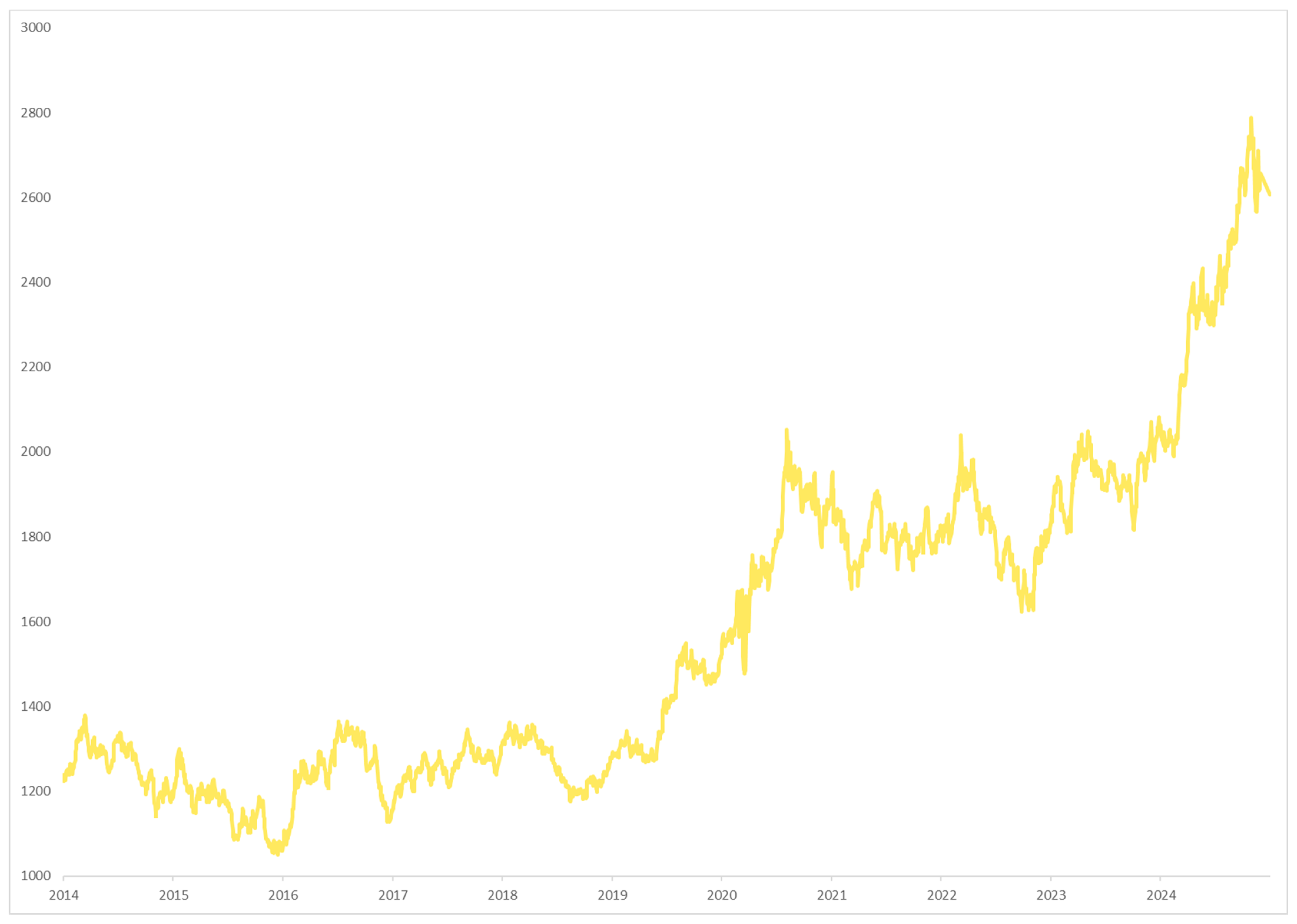
Figure A2.
Financial indicators over time.
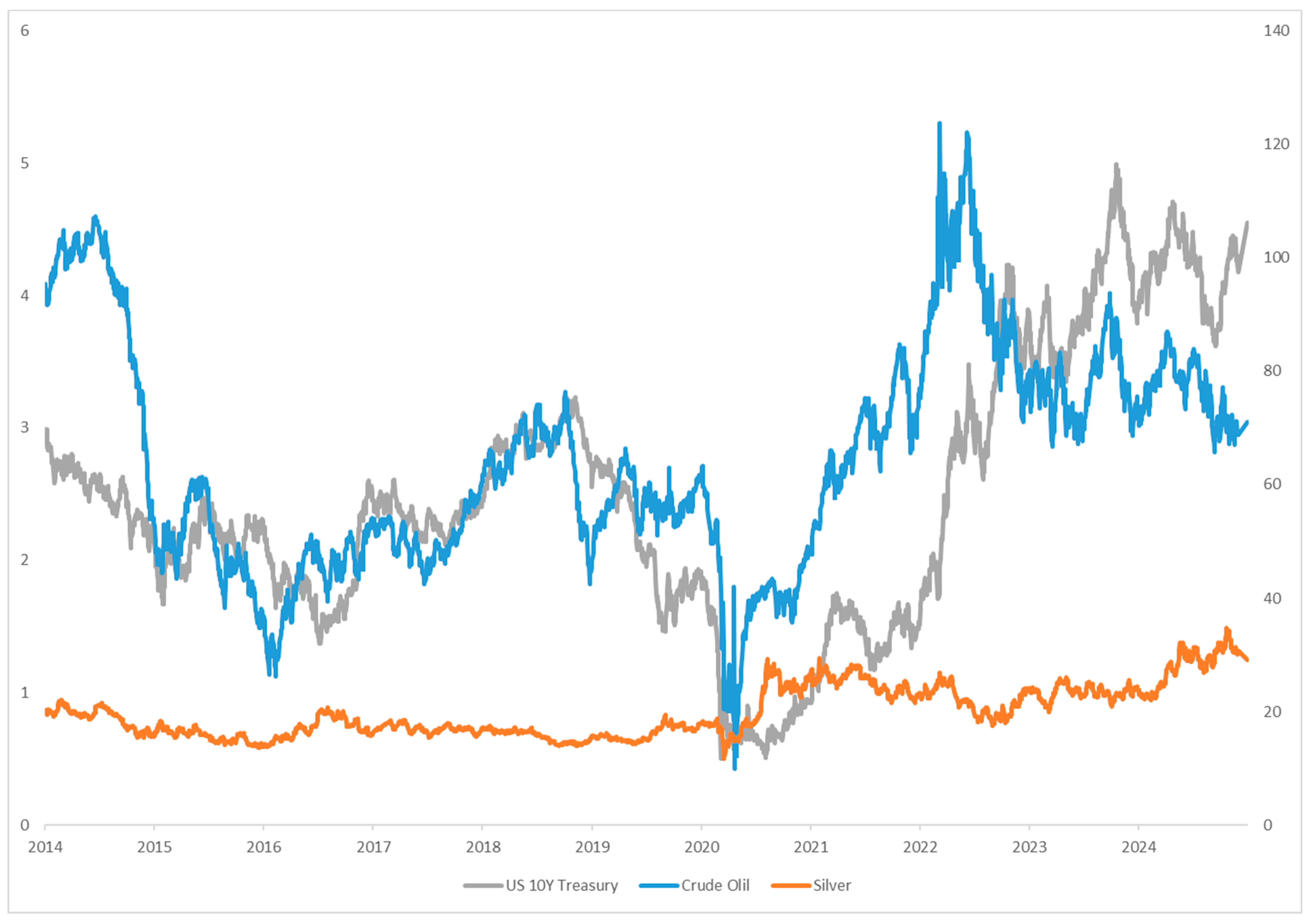
Figure A3.
Macroeconomic indicators over time.
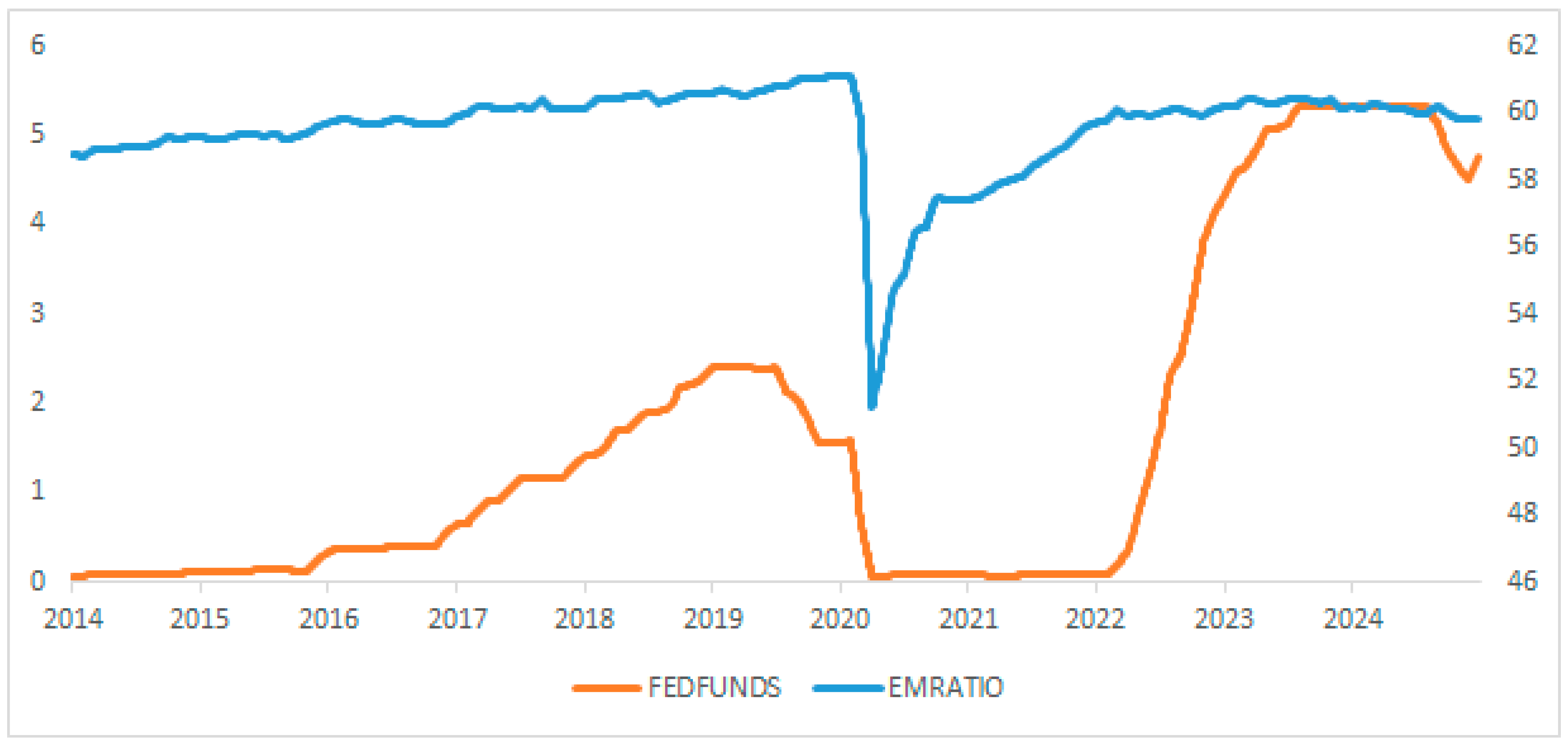
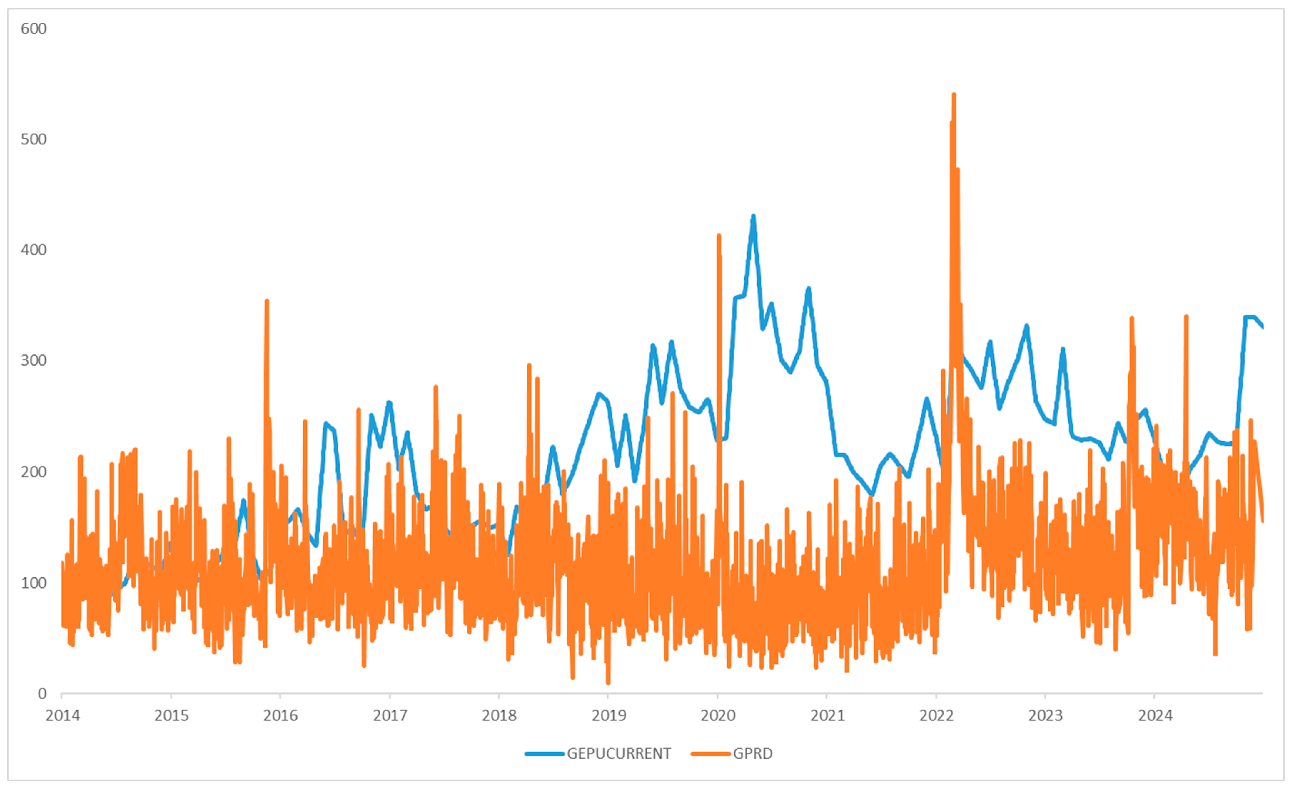
Figure A4.
Sentiment metrics over time.
References
- (Adebiyi et al., 2014) Adebiyi, A. A., Adewumi, A. O., & Ayo, C. K. (2014). Comparison of ARIMA and artificial neural networks models for stock price prediction. Journal of Applied Mathematics, 2014(1), 614342. [CrossRef]
- (Amini & Kalantari, 2024) Amini, A., & Kalantari, R. (2024). Gold price prediction by a CNN-Bi-LSTM model along with automatic parameter tuning. PLOS ONE, 19(3), e0298426. [CrossRef]
- (Baker et al. 2025) Baker, Bloom & Davis Economic Policy Uncertainty Index. Available online: https://www.policyuncertainty.com (last accessed on 17 April 2025).
- (Baur & Smales, 2020) Baur, D. G., & Smales, L. A. (2020). Hedging geopolitical risk with precious metals. Journal of Banking & Finance, 117, 105823. [CrossRef]
- (Beckmann et al., 2019) Beckmann, J., Berger, T., & Czudaj, R. (2019). Gold price dynamics and the role of uncertainty. Quantitative Finance, 19(4), 663–681. [CrossRef]
- (Bottou, 2010) Bottou, L. (2010). Large-scale machine learning with stochastic gradient descent. In Proceedings of COMPSTAT'2010: 19th International Conference on Computational Statistics, Paris, France, August 22–27, 2010 Keynote, Invited and Contributed Papers (pp. 177–186). Physica-Verlag HD. [CrossRef]
- (Breiman, 2001) Breiman, L. (2001). Random forests. Machine Learning, 45, 5–32. [CrossRef]
- (Caldara & Iacoviello, 2022) Caldara, D., & Iacoviello, M. (2022). Measuring geopolitical risk. American economic review, 112(4), 1194–1225.
- (Cho et al., 2014) Cho, K., Van Merriënboer, B., Gulcehre, C., Bahdanau, D., Bougares, F., Schwenk, H., & Bengio, Y. (2014). Learning phrase representations using RNN encoder-decoder for statistical machine translation. arXiv preprint arXiv:1406.1078.
- (CME Group, 2025) Gold Futures – Volume & Open Interest. Available online: https://www.cmegroup.com/markets/metals/precious/gold.volume.html (accessed on 15 April 2025).
- (Fang et al., 2018) Fang, L., Yu, H., & Xiao, W. (2018). Forecasting gold futures market volatility using macroeconomic variables in the United States. Economic Modelling, 72, 249–259. [CrossRef]
- (Fischer & Krauss, 2018) Fischer, T., & Krauss, C. (2018). Deep learning with long short-term memory networks for financial market predictions. European Journal of Operational Research, 270(2), 654–669. [CrossRef]
- (Gold Trading Platforms, 2024) The Rise of Digital Gold Trading Platforms: How Technology is Changing the Investment Landscape. November 2024. Available online: https://www.isabullion.com/articles/the-rise-of-digital-gold-trading-platforms-how-technology-is-changing-the-investment-landscape/ (accessed on 15 April 2025).
- (Granger, 1969) Granger, C. W. (1969). Investigating causal relations by econometric models and cross-spectral methods. Econometrica: Journal of the Econometric Society, 424–438. [CrossRef]
- (Graves & Schmidhuber, 2005) Graves, A., & Schmidhuber, J. (2005). Framewise phoneme classification with bidirectional LSTM and other neural network architectures. Neural Networks, 18(5–6), 602–610. [CrossRef]
- (Gür, 2024) Gür, Y. E. (2024). Comparative analysis of deep learning models for silver price prediction: CNN, LSTM, GRU and hybrid approach. Akdeniz İİBF Dergisi, 24(1), 1–13. [CrossRef]
- (Hajek & Novotny, 2022) Hajek, P., & Novotny, J. (2022). Fuzzy rule-based prediction of gold prices using news affect. Expert Systems with Applications, 193, 116487. [CrossRef]
- (Hamilton, 1989) Hamilton, J. D. (1989). A new approach to the economic analysis of nonstationary time series and the business cycle. Econometrica, 57(2), 357–384. [CrossRef]
- (Hochreiter & Schmidhuber, 1997) Hochreiter, S., & Schmidhuber, J. (1997). Long short-term memory. Neural Computation, 9(8), 1735–1780. [CrossRef]
- (Hyndman & Athanasopoulos, 2021) Hyndman, R. J., & Athanasopoulos, G. (2021). Forecasting: Principles and practice (3rd ed.). OTexts: Melbourne, Australia. Available online: https://otexts.com/fpp3/ (accessed on 15 April 2025).
- (LeCun et al., 2015) LeCun, Y., Bengio, Y., & Hinton, G. (2015). Deep learning. Nature, 521(7553), 436–444. [CrossRef]
- (Liang et al., 2022) Liang, Y., Lin, Y., & Lu, Q. (2022). Forecasting gold price using a novel hybrid model with ICEEMDAN and LSTM-CNN-CBAM. Expert Systems with Applications, 206, 117847. [CrossRef]
- (Lundberg & Lee, 2017) Lundberg, S. M., & Lee, S.-I. (2017). A Unified Approach to Interpreting Model Predictions. Advances in Neural Information Processing Systems, 30. https://proceedings.neurips.cc/paper_files/paper/2017/file/8a20a8621978632d76c43dfd28b67767-Paper.pdf.
- (Mamoudan et al., 2023) Mamoudan, M. M., Ostadi, A., Pourkhodabakhsh, N., Fathollahi-Fard, A. M., & Soleimani, F. (2023). Hybrid neural network-based metaheuristics for prediction of financial markets: A case study on global gold market. Journal of Computational Design and Engineering, 10(3), 1110–1125. [CrossRef]
- (O'Brien, 2007) O'Brien, R. M. (2007). A caution regarding rules of thumb for variance inflation factors. Quality & Quantity, 41(5), 673–690. [CrossRef]
- (Pokou et al., 2024) Pokou, F., Sadefo Kamdem, J., & Benhmad, F. (2024). Hybridization of ARIMA with learning models for forecasting of stock market time series. Computational Economics, 63(4), 1349–1399. [CrossRef]
- (Qiu et al., 2024) Qiu, C., Zhang, Y., Qian, X., Wu, C., Lou, J., Chen, Y., … & Gong, Z. (2024). A two-stage deep fusion integration framework based on feature fusion and residual correction for gold price forecasting. IEEE Access. [CrossRef]
- (Raza et al., 2018) Raza, S. A., Shah, N., & Shahbaz, M. (2018). Does economic policy uncertainty influence gold prices? Evidence from a nonparametric causality-in-quantiles approach. Resources Policy, 57, 61–68. [CrossRef]
- (Reboredo, 2013) Reboredo, J. C. (2013). Is gold a hedge or safe haven against oil price movements? Resources Policy, 38(2), 130–137. [CrossRef]
- (Ribeiro et al., 2016) Ribeiro, M. T., Singh, S., & Guestrin, C. (2016). Why Should I Trust You?": Explaining the Predictions of Any Classifier. Proceedings of the 22nd ACM SIGKDD International Conference on Knowledge Discovery and Data Mining, 1135–1144. [CrossRef]
- (Shi et al., 2015) Shi, X., Chen, Z., Wang, H., Yeung, D. Y., Wong, W. K., & Woo, W. C. (2015). Convolutional LSTM network: A machine learning approach for precipitation nowcasting. Advances in Neural Information Processing Systems, 28.
- (Smola & Schölkopf, 2004) Smola, A. J., & Schölkopf, B. (2004). A tutorial on support vector regression. Statistics and Computing, 14, 199–222. [CrossRef]
- (Stanković et al., 2023) Stanković, M., Bačanin, N., Budimirović, N., Živković, M., Sarač, M., & Štrumberger, I. (2023, April). Bi-directional long short-term memory optimization by improved teaching-learning based algorithm for univariate gold price forecasting. In 2023 International Conference on Inventive Computation Technologies (ICICT) (pp. 1650–1657). IEEE. [CrossRef]
- (Tashakkori et al., 2024) Tashakkori, A., Talebzadeh, M., Salboukh, F., & Deshmukh, L. (2024). Forecasting gold prices with MLP neural networks: A machine learning approach. International Journal of Science and Engineering Applications (IJSEA), 13, 13–20. https://doi.com/10.7753/IJSEA1308.1003.
- (Taylor & Letham, 2018) Taylor, S. J., & Letham, B. (2018). Forecasting at scale. The American Statistician, 72(1), 37–45. [CrossRef]
- (WGC, 2025) World Gold Council. Gold Demand Trends: Full Year 2024. Available online: https://www.gold.org/goldhub/research/gold-demand-trends/gold-demand-trends-full-year-2024 (accessed on 15 April 2025).
- (Zangana & Obeyd, 2024) Zangana, H. M., & Obeyd, S. R. (2024). Deep learning-based gold price prediction: A novel approach using time series analysis. Sistemasi: Jurnal Sistem Informasi, 13(6), 2581–2591. https://sistemasi.org/index.php/stmsi/article/view/4651.
Figure 1.
Flowchart of the proposed hybrid framework for gold price prediction.
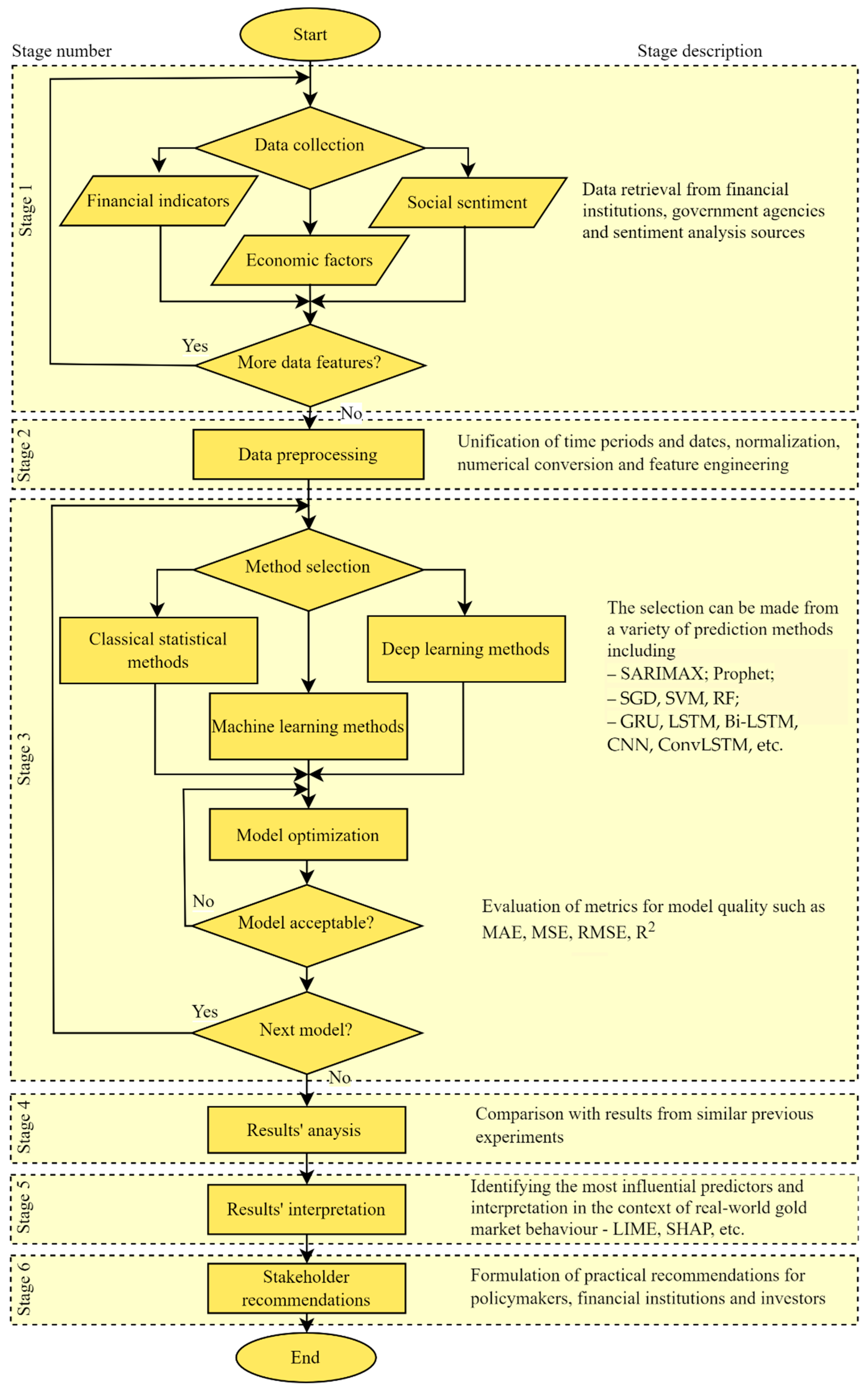
Figure 2.
Actual vs. predicted gold prices on the test set – Prophet model.
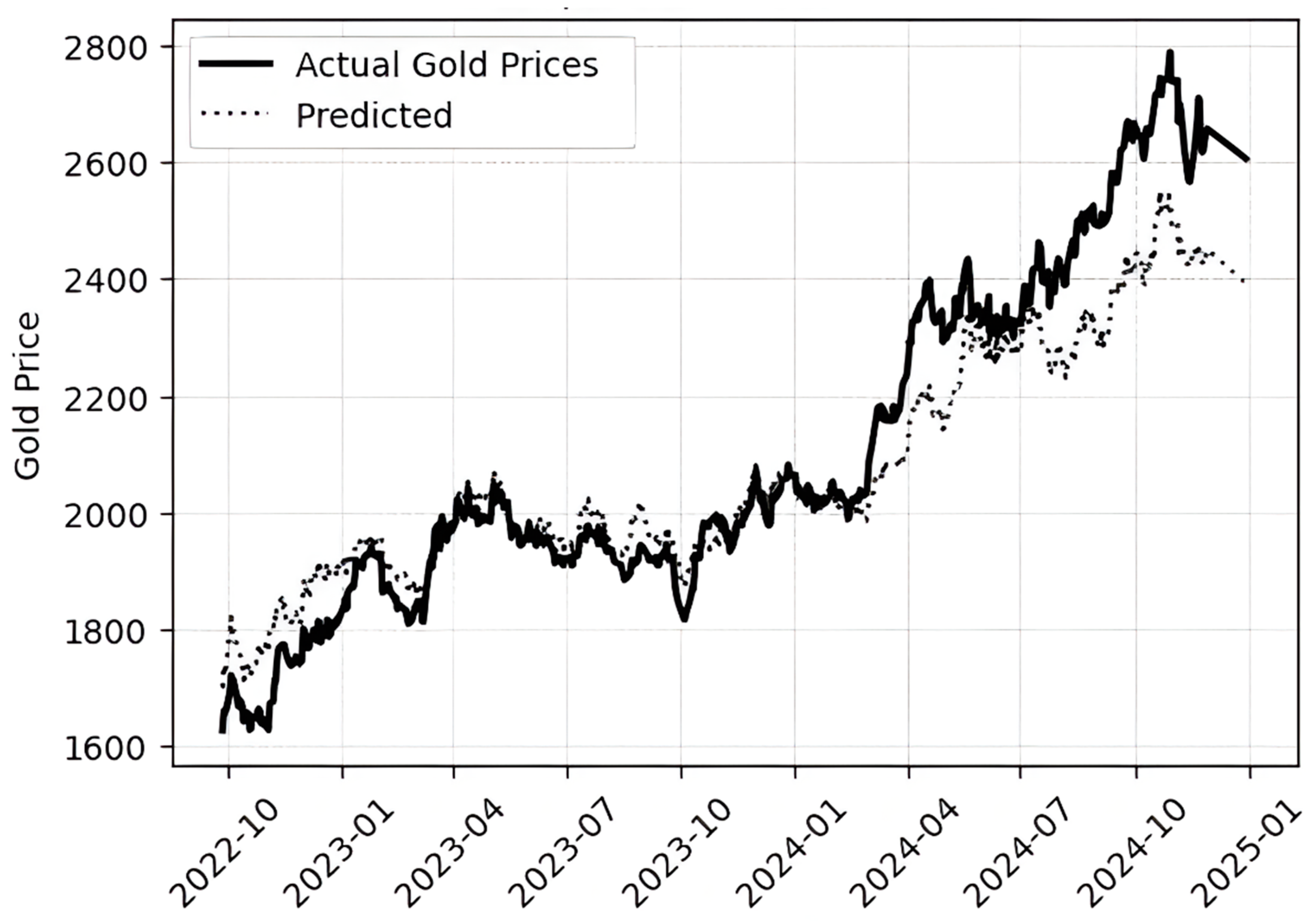
Figure 3.
SHAP feature importance plot – BiLSTM forecasting model.
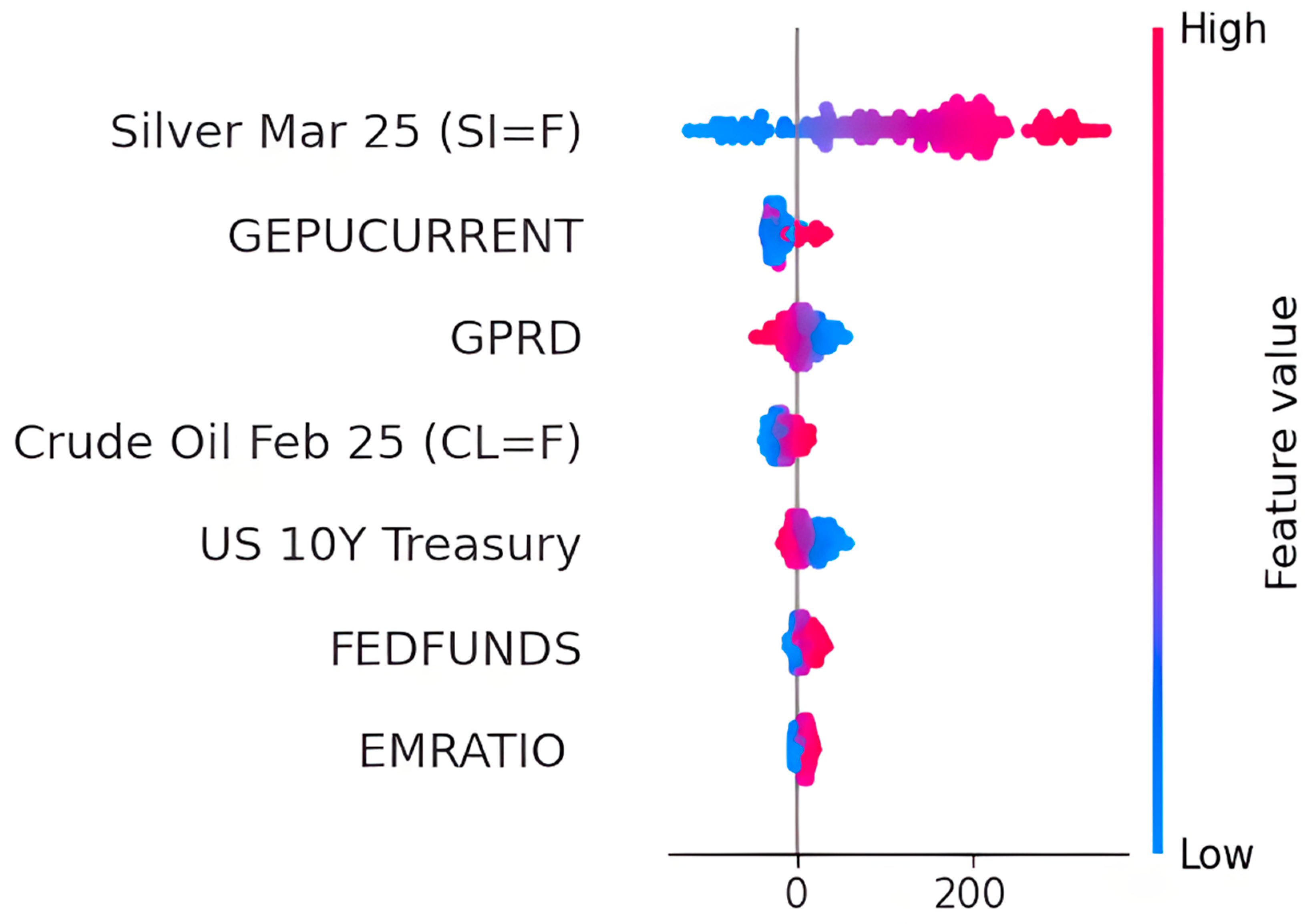
Table 1.
Summary of recent studies on gold price forecasting.
| Reference | Research objective | Dataset characteristics | Prediction methods |
Model evaluation |
|---|---|---|---|---|
| Hajek & Novotny, 2022 | Framework for gold price prediction using different indicators and news sentiment | Gold futures, financial indicators, news sentiment (2007–2017) | FURIA with evolutionary tuning | Accuracy, AUC, interpretability via IF–THEN fuzzy rules |
| Liang et al., 2022 | Hybrid DL-based prediction method | Gold futures and spot prices (2010–2020) | ICEEMDAN + LSTM + CNN + CBAM | MAE1, MSE2, RMSE3, MAPE4, SMAPE5 in MCS test |
| Mousapour Mamoudan et al., 2023 | Hybrid DL-based method using trading signals from technical indicators | 112 features from MACD, Ichimoku, MA indicators (10 months of 2020) | CNN + BiGRU, optimized by FA, MFO, PSO, and GA | Accuracy, Precision, Recall, F1, ROC-AUC |
| Stanković et al., 2023 | Hybrid DL-based method with trend extraction and hyperparameter optimization procedure | Gold prices (2020–2022) | VMD + BiLSTM + ITLB | MAE, MSE, RMSE, R² 6 |
| Amini & Kalantari, 2024 | Hybrid DL-based method with parameter tuning | Gold prices (1978–2021) | CNN + BiLSTM | MSE, RMSE, MAE, R² |
| Gür, 2024 | Hybrid DL-based model for silver prices prediction with grid search optimization | Silver prices (2017–2023) | CNN + LSTM + GRU | RMSE, MAE, MAPE, R², MASE7 |
| Pokou et al., 2024 | Hybrid ARIMA+ML methods | Gold prices (2016–2023, three periods) | ARIMA + ML combinations | RMSE, MAPE, NSE8 |
| Qiu et al., 2024 | DL framework with features fusion and residual correction | Four gold futures series (2004–2022) | VMD + BP + CNN + LSTM | MSE, MAE, RMSE, R2, MAPE |
| Tashakkori et al., 2024 | MLP-based model using gold trading features | Gold trading indicators OHLCV (2012– 2022) | MLP | Test error |
| Zangana & Obeyd, 2024 | Two LSTM variants with explainability | Gold prices and macroeconomic data (oil, USD/EUR, inflation, interest) | LSTM, BiLSTM, SHAP | MAE, RMSE, R² |
1 MAE – Mean Absolute Error, 2 MSE – Mean Squared Error, 3 RMSE – Root Mean Squared Error, 4 MAPE – Mean Absolute Percentage Error, 5 sMAPE – symmetric Mean Absolute Percentage Error, 6 R2 – Coefficient of Determination, 7 MASE – Mean Absolute Scaled Error, 8 NSE – Nash-Sutcliffe Efficiency.
Table 2.
Forecasting performance of models on the test set.
| Model | MAE | RMSE | R2 |
|---|---|---|---|
| SARIMAX | 148.75 | 185.31 | 0.577 |
| SGD | 190.96 | 229.21 | 0.353 |
| Prophet | 76.30 | 102.34 | 0.871 |
| GRU | 201.07 | 222.53 | 0.390 |
| LSTM | 129.67 | 159.05 | 0.688 |
| BiLSTM | 113.65 | 145.60 | 0.739 |
| CNN | 181.30 | 227.17 | 0.364 |
| ConvLSTM | 199.03 | 227.23 | 0.364 |
Disclaimer/Publisher’s Note: The statements, opinions and data contained in all publications are solely those of the individual author(s) and contributor(s) and not of MDPI and/or the editor(s). MDPI and/or the editor(s) disclaim responsibility for any injury to people or property resulting from any ideas, methods, instructions or products referred to in the content. |
© 2025 by the authors. Licensee MDPI, Basel, Switzerland. This article is an open access article distributed under the terms and conditions of the Creative Commons Attribution (CC BY) license (http://creativecommons.org/licenses/by/4.0/).
Copyright: This open access article is published under a Creative Commons CC BY 4.0 license, which permit the free download, distribution, and reuse, provided that the author and preprint are cited in any reuse.


