
Submitted:
19 April 2025
Posted:
21 April 2025
You are already at the latest version
Abstract
We present a theoretical framework for designing optical masks useful for implementing Schlieren techniques. We revisit the use of effective transfer functions, for emphasizing the role of masks symmetries. We unveil a statistical model describing phase gradients as randomly located prisms. We disclose the use of two similar coding masks for implementing a Schlieren technique, based on optical autocorrelations. One mask covers the source, and the other mask acts as a spatial filter. We exploit the properties of the Barker sequences, for achieving highly peaked noncyclic autocorrelations. This operation leads to the design of an automatic sensor for phase gradients.
Keywords:
Schlieren techniques
; Foucault test
; Barker sequences
; Optical Autocorrelations
1. Introduction
For current applications in optical microscopy and optical testing, researchers have developed techniques for rendering visible transparent structures [1,2,3,4]. Among others, we note Foucault’s remarkable invention of the knife-edge.
This optical technique initiated experimental methods for testing optical elements. visualizing the departures of sphericity of mirrors and lenses [5].
According to Krehl and Engemann [6], independently of Foucault, Toepler was the first person who visualized shock waves, by employing a knife-edge [7].
Renitz also noted that there is an early version of the knife-edge [8]. Furthermore, Renitz has also recognized previous experimental results from Wiesel and Marat [9].
Zernike presented the phase contrast technique for microscopy as an improved version of the knife-edge technique [10]. Independently of Zernike, Lyot proposed a phase contrast technique, used for visualizing polishing inhomogeneities in a coronagraph [11].
Due to the contributions of Schardin [12] and Burton [13], the use of the knife-edge is now recognized as a member of the Schlieren techniques [14,15,16,17].
Here, for implementing nonconventional Schlieren techniques, we unveil the use of 1-D optical masks, coded either with the Barker sequences [18], or with the pseudorandom sequences [19].
For developing our current discussion, in Section 2, we revisit the basics of an effective transfer function, which was initially proposed by Menzel [20,21]. This concept was further developed by one of us [22,23,24,25]. This discussion considers, as input pattern, a transparent grating that has weak phase variations.
For emphasizing the usefulness of the transfer function, in Section 3, we present a statistical model, which describes the presence of a randomly located prism.
In Section 4, we discuss the usage of a coded source. We note that there is a link between the Schlieren techniques and the mathematical expression for the ambiguity functions, as employed in RADAR engineering [26,27,28,29,30]. We disclose the use of optical autocorrelations for implementing Schlieren techniques.
2. Effective Transfer Function
In Figure 1, we depict the schematics of an optical processor, which is used for describing our proposal.
In Figure 1, the input pattern is placed in the axis denoted as x’. The input pattern is a sinusoidal phase grating, with period d. Its complex amplitude transmittance is
In Equation (1) the amplitude of the phase delays is denoted with the lower-case Latin Letter a. And the upper-case Greek letter λ denotes the wavelength. Next, we consider that the above grating has phase variations that are weak, in the sense that
Under this assumption, the complex amplitude transmittance can be approximated by the initial two terms of its Taylor expansion. Hence, we consider that the input patterns have the following complex amplitude transmittance
The Fourier spectrum of Equation (2) is
In Equation (3), the Greek letters, μ and ν denote the spatial frequencies at Fourier domain. We note that the mathematical expression in Equation (3) represents the complex amplitude distribution impinging on the optical mask. If we denote as the amplitude transmittance of the optical mask, then after the mask the amplitude transmittance reads
By taking an inverse Fourier transformation of Equation (4), we obtain the complex amplitude distribution at the image plane. That is,
Here, it is convenient to recognize that can be expressed in a unique manner as the sum of two functions. The function is an even function. And the function is an odd function. For further details, please see Appendix A.
In Figure 2, we depict the even component, , and the odd component, , of the amplitude transmittance of the function
If we substitute Equation (6) in Equation (5) we have that
The definition of the normalized image irradiance distribution is
From Equations (7) and (8) we obtain the normalized image irradiance distribution
Now, it is relevant to make the following comparison between Equations (2) and (9). The complex amplitude distribution at the input plane, in Equation (2), is mapped as an image irradiance distribution, in Equation (9). The initial sinusoidal variation is transferred as a cosinusoidal variation, with modulation that is equal to
In other words, there is a spatial frequency mapping, which can be associated with an effective transfer function, which is sampled at the spatial frequency 1/d. This remarkable simple result is conveniently depicted in Figure 3.
Furthermore, it is apparent from Equation (10) that the action of effective transfer function can be enhanced if the value at the origin of the even component, E(0), is less than unity. This observation is useful for proposing improvements to two previous Schlieren techniques, which are depicted in Figure 2. For Wolter’s phase edge, the coded mask has the following amplitude transmittance
In Equation (11), the Greek letter Ω denotes the cut-off spatial frequency. In Figure 4a we plot Equation (11). Now, for the modulation contrast technique [31], the amplitude transmittance is
In Equation (12), the Greek letters α and ε denote two real numbers with values lower than unity. The letter α represents an attenuation coefficient at the center of the mask. And the letter ε indicates the length covered by the central section, as compared with the length covered by the mask.
In Figure 4 , we plot the amplitude for an improved version, which incorporates a transmission equals minus unity; as in Wolter’s phase edge. And it also incorporates a central attenuation coefficient, as in the modulation contrast technique. Its amplitude distribution reads
Next, we note that some authors use, in a lax manner, a heuristic approach for describing phase gradients. This description considers that a phase gradient is a randomly located prism. To our knowledge, this heuristic approach has not been described in terms of scalar diffraction. For gaining physical insight, on the heuristic approach, we present next a diffraction-based description.
3. Randomly Located Prism
In Equation (14) we denote the amplitude transmittance of a prism that has a random location. That is,
In Equation (14) the random variable X takes values that obey to a probability density function p(X). Its Fourier transform pair is the characteristic function
Under the assumption of weak phase delays, we can approximate Equation (14) as follows
Its Fourier spectrum reads
After passing through the coding mask, Q(μ, ν), the Fourier spectrum reads
By substituting Equation (17) in Equation (18) we obtain the explicit expression
Next, as discussed in Appendix B, we take the ensemble average of Equation (19). The average Fourier spectrum is
Then, we recognize the convenience of defining the transfer function
The characteristic function is assumed to be an even function. Then, the even component of has the following expression
And the odd even component of has the following form
Consequently, Equation (20) can be written as
As discussed in Appendix B, the average complex amplitude distribution is
And as noted in Appendix B, the average irradiance distribution is
From Equation (26) and from Figure 5, we observe two relevant features. The presence of a randomly located prism is imaged as a uniform average irradiance distribution, plus a term that contains the phase modulation caused by the prism.
In other words, the phase gradient is rendered visible, as an irradiance variation, due to the presence of the function Hence, like Equation (10), it is convenient define the following effective transfer function
From Equations (23) and (27), we claim that the effective transfer function is the product of a characteristic function times the odd component of coding mask. And consequently, as depicted in Figure 5, the current effective transfer function has now an apodizing effect. To our knowledge, this is a novel formulation.
4. Coded Source: An Imaging Process
We note the existence of heuristic descriptions for considers a transparent structure as a set of randomly located prisms. This heuristic description ignores any discussions on scalar diffraction. For rectifying this limitation, next we develop an imaging process, which considers a coded source. As part of our rationale, we consider first a simple case. As depicted in Figure 6, we consider the source as a slit. At its conjugated image, (μ, ν), we place a second slit that acts as the spatial filter.
In the absences of phase gradients, the two slits coincide. And the light throughput achieves its maximum value. On the other hand, if a phase gradient is present then the image of the source is laterally shifted (say by the amount ζ / λ). This mismatch generates a drop light throughput. That is,
In Equation (28), the Greek letter omega denotes the width of the slit used to cover the source. If one evaluates Equation (28), then one obtains
It is apparent from Equation (29) that the light throughput varies slowly with the variable ζ, except for a very narrow slit. However, the light throughput is reduced if one uses narrows slits. Hence, we search next for other options. To conclude, we consider that the source is coded with multiple slits. Then, at the source plane the amplitude transmittance is
In Equation (30) the Greek letters μ’ and ν’ denote spatial frequency coordinates at the source plane. At the input plane, the coordinates we employ the coordinates x’ and y’. At this plane, the amplitude distribution is the Fourier transform of Equation (30). That is,
In Equation (31) the function is the 1-D Fourier spectrum of the coded source. Next, we consider that a prism alters the amplitude distribution in Equation (28). Then, the new amplitude distribution reads
In Equation (32) we consider the presence of a weak phase gradient. Its deflection angle is denoted with the Greek letter ζ. The amplitude distribution, at the pupil aperture, is the inverse Fourier transform of Equation (32). That is,
Next, we consider that the amplitude distribution, in Equation (33), impinges on a second coded mask. For this application, the second mask acts as the spatial filter. Its amplitude transmittance is Q*(μ). Then, just after the mask, the amplitude transmittance is
It is straightforward to substitute Equation (33) in Equation (34), for obtaining
As expected, at the pupil aperture, the amplitude distribution is a product between a lateral shifted version of the coded source, times the complex conjugate transmittance of the coded mask. And consequently, at the image plane the amplitude distribution is
The mathematical expression in Equation (36) is like the definition of the ambiguity function, as is used in RADAR engineering. This is a previously unknown feature of the Schlieren masks. However, any further discussion on this topic is beyond our current scope. We observe that Equation (36), at the origin (x =0, y = 0), is the light throughput T in Equation (28). That is,
From Equation (37) we state the following working hypothesis. By coding the source as well as the spatial filter with the same sequence, its autocorrelation usefully detects phase gradients. This working hypothesis leads us to the following proposal.
5. Optical Visualization and Automatic Detection
Since a pseudorandom sequence or a Barker sequence have sharp autocorrelations, then they can be useful for automatically detecting phase gradients. For elaborating on this working hypothesis, we note that either the pseudorandom sequences, or the Barker sequences have a finite number of elements, say L. This integer number L is denoted as the sequence length. In electronics, the sequences are commonly employed as cyclic sequences. However, in optics, due to the finite size of the mask the coding sequences are noncyclic. Next, we elaborate on this difference.
The pseudorandom sequences exhibit a high peak over an otherwise uniform value, as depicted in Figure 7. In this pictorial, we show two examples of the pseudorandom sequences. In these sequences the amplitude transmittance has values that are equal to unity, or equal to zero. In Figure 7a, the length is L = 7. And in (b) the length is L = 15. These examples were selected for making comparisons with the results of other authors [32].
In Figure 8, we show the cyclic autocorrelations associated with the sequences in Figure 7. The autocorrelations exhibit peaks that overshoot a uniform value.
In Figure 9, we show that the Barker sequences of length L = 7 and L = 13.Now, the amplitude transmittance has values equal to unity, or equal to minus unity.
In Figure 10, we plot the cyclic autocorrelation associated with the sequences in Figure 9. It is apparent from Figure 10 that the autocorrelations also have peaks that overrun the values of the adjacent sidelobes. The peaks baselines narrow down from the length L = 7 to the length L = 13.
As previously indicated, in optics one is dealing with noncyclic autocorrelations. This is due to the finite size of the masks. The autocorrelations do not repeat themselves. To visualize the impact of this feature, we present the noncyclic autocorrelations of the pseudo random sequences, as well as the noncyclic autocorrelations of the Barker sequences.
From Figure 11 and from Figure 12, we note that the noncyclic autocorrelations do not have replicated peaks. Furthermore, associated with the pseudorandom sequences, the noncyclic autocorrelations exhibit sidelobes variable values.
From Figure 12, we observe that the Barker sequences generate noncyclic autocorrelations, which exhibit a distinctives central peak, with replicated sidelobes. Hence, Barker codes can be a desirable choice implementing an automatic sensor, based on optical autocorrelations. In the absence of phase gradients, the noncyclic autocorrelations have a central distinctives peak. On the other hand, if there are phase gradients, then the noncyclic autocorrelations have reduced values.
For the implementation of an automatic sensor, one has two choices. In Figure 13a, we show an unfolded version of the sensor. optical setup is shown in Figure 13a. And in Figure 13b, we depict folded optical setup.
Hence, Barker codes can be a desirable choice for coding the source and the spatial filter. And in this manner one can have a correlation method for automatically detecting the presence of phase gradients. For this purpose, the optical setup is shown in Figure 13. An unfolded version of the optical setup is shown in Figure 13a. And in Figure 13b, we use a spherical mirror for depicting a folding version of the optical setup.
6. Conclusions
We have described a theoretical framework for designing nonconventional Schlieren techniques. These techniques employ optical masks for rendering visible phase gradients, like the Foucault knife-edge.
We have revisited the use of an effective transfer function. This discussion clarifies the relevance of employing arguments of symmetry, when designing Schlieren techniques.
We have disclosed a statistical model that describes phase gradients as randomly located prisms.
We have unveiled a link between the generation of optical autocorrelations and the use of Schlieren techniques. We employ two masks that at geometrical optics conjugates planes. The first mask is for coding the source. And a second mask is for coding the spatial filter. In this manner, we obtain a Schlieren technique with high light throughput.
We have indicated that the use of two masks is linked to the implementation of an optical correlator. This link is useful for implementing an automatic method that detects phase gradients.
The optical correlator exploits the use of Barker sequences for generating highly peaked, noncyclic irradiance distributions.
Author Contributions
Conceptualization, JOC; methodology, JOC; software, CMGS.; validation, JOC., and CMGS; writing—original draft preparation, JOC; writing—review and editing, CMGS. All authors have read and agreed to the published version of the manuscript.
Data Availability Statement
Currently, we do not include the numerical procedures for evaluating the graphs and the figures in this paper.
Acknowledgments
We express our gratitude to the National Research Council of Science, Humanities and Innovation for supporting scholarships.
Conflicts of Interest
The authors declare no conflicts of interest.
Appendix A: Symmetry Considerations
As pointed out in Equation (), we write the amplitude transmittance as the sum of an even function and of an odd function
One finds the even function by using the formula
By substituting Equation (A1) in Equation (5) we have that
Equation (A4) can also be written as
Equation (A5) appears as Equation (7) in the main text.
Appendix B: Statistical Considerations
We use a Fourier transform for expressing the even component in Equation (19) as follows
We note that the function is a real, even function of the variable x. We note that the odd component, in Equation (20), is a real function. Its Fourier transform is also an odd function. However, its Fourier transform is a purely imaginary function. Hence, it is convenient to use the following expression
Thus, at the image plane, the average amplitude distribution is
Or equivalently, the average amplitude distribution is
Next, we use the following definition for the normalized, average irradiance distribution
By substituting Equation (B4) in Equation (B5) we have that
Equation(B6) appears as Equation (9) in the main text.
References
- Daria V., Glückstad J., Mogensen P. C., Eriksen R. L., and Sinzinger S., Implementing the generalized phase-contrast method in a planar-integrated micro-optics platform, Opt. Lett. 2002, 27: 945-947. [CrossRef]
- Teschke M. and Sinzinger S., Modified phase contrast for recording of holographic optical elements, Opt. Lett. 2007, 32: 2067-2069. [CrossRef]
- Teschke M., Heyer R., Fritzsche M., Stoebenau S., and Sinzinger S., Application of an interferometric phase contrast method to fabricate arbitrary diffractive optical elements, Appl. Opt. 2008, 47: 2550-2556. [CrossRef]
- Teschke M., and Sinzinger S., Phase contrast imaging: a generalized perspective, J. Opt. Soc. Am. A 2009, 26: 1015. [CrossRef]
- Foucault, L., Description des procédées employés pour reconnaître la configuration des surfaces optiques, Comptes rendus hebdomadaires des séances de l’Académie des Sciences 1858, 47: 958–959.
- Krehl, P., Engemann, S., August Toepler: the first who visualized shock waves, Shock Waves 1995, 5: 1–18. [CrossRef]
- Toepler, A., Beobachtungen nach einer Neuen Optischen Methode, Poggendorf’s Annalen der Physik und Chemie 1866, 127: 556-580.
- Reinitz J., Schlieren experiment 300 years ago, Nature 1975, 254: 293-295. [CrossRef]
- Reinitz J., Optical inhomogeneities: Schlieren and shadowgraph methods in the seventeenth and eighteenth centuries, Endeavour 1997, 21: 77-81. [CrossRef]
- Zernike F., Diffraction theory of the knife-edge test and its improved form, the phase-contrast method, Mon. Not. R. Astron. Soc. 1934, 94: 377-384.
- Lyot B., Procèdes Perme Hand d’Etudier les Irrégularités d’une Surface Optique Bien Polie, C. R. Acad. Sci. 1946, 222, 765.
- Schardin H., Die Schlierenverfahren und ihre Anwendungen Ergebnisse der Exakten Naturwissenschaften 1942, 20: 303–439.
- Burton, R. A., A modified schlieren apparatus for large areas of field, J. Opt. Soc. Am. 1949, 39: 907-908. [CrossRef]
- Wolter H., Schlieren-Phase Kontrast und Lichtschnittverfahren, in Handbuch der Physik 24, Springer-Verlag: Berlin, 1956, 555–645. [CrossRef]
- Davies P. T., Schlieren photography - short bibliography and review, Opt. Laser Tech. 1981, 30: 37-42. [CrossRef]
- Settles G. S., and Hargather M. J., A review of recent developments in schlieren and shadowgraph techniques, Meas. Sci. Technol. 2017, 28: 1-25. [CrossRef]
- Ojeda-Castaneda J., A proposal to classify methods employed to detect thin phase structures under coherent illumination, Opt. Acta 27: 917–929 (1980). [CrossRef]
- Barker R. H., Group synchronizing of binary digital systems, in Communication Theory, Butterworth: London, 1953, 273-287.
- Harwit, M, and Sloane, N. J. A., Hadamard transform optics, Academic Press: New York, 1979, 200-2005.
- Menzel E., Die Darstellung verschiedener Phasekontrast Verfahren in der Optischen Ubertragungstheori, Optik (Stuttgart) 1958, 15: 460–470.
- Menzel E., Transfer-functions in optics, Optik (Stuttgart) 1973, 39: 170–172.
- Ojeda-Castaneda J., Necessary and sufficient conditions for thin phase imagery, Opt. Acta 1980, 27, 905–915. [CrossRef]
- Ojeda-Castaneda J., and L. R. Berriel-Valdos L. R., Classification scheme and properties of Schlieren techniques, Appl. Opt. 1979, 18: 3338–3341 (1979). [CrossRef]
- Ojeda-Castaneda J., Chapter 5, Foucault wire and phase modulation tests, edited by D. Malacara, Optical Shop Testing, John Wiley: New York 1992, 265-320.
- Gómez-Sarabia C. M., and Jorge Ojeda-Castaneda J., Schlieren masks: square root monomials, sigmoidal functions, and off-axis Gaussians, Appl. Opt. 2020, 59: 3589-3594. [CrossRef]
- Woodward, P. M., Probability and information theory with application to radar, Pergamon: Oxford 1953, 115-125.
- Papoulis, A., Ambiguity function in Fourier optics, J. Opt. Soc. Am. 1974, 64, 779 – 788. [CrossRef]
- Guigay, J.- P., The ambiguity function in diffraction and isoplanatic imaging by partially coherent beams, Opt. Comm. 1978, 26, 136-138. [CrossRef]
- Ojeda-Castañeda, J., Lancis, J., Gómez-Sarabia, C. M., Torres-Company, J., and Andrés, P. Ambiguity function analysis of pulse train propagation: applications to temporal Lau filtering. J. Opt. Soc. Am. A 2007, 24, 2268–2273. [CrossRef]
- Ojeda-Castañeda, J., Wavefront Shaping and Pupil Engineering, Springer-Verlag: Berlin, 2021, 135-253.
- Hofmann R., and Gross L., Modulation Contrast Microscope, Appl. Opt. 1975, 14: 1169–1176. [CrossRef]
Figure 1.
Schematics of the optical setup under consideration. The spatial filter is located pupil at the axis, denoted with the Greek letter μ. This axis is the geometrical optics conjugate of the source axis, μ’. In (a) a knife edge acts as the spatial filter. In (b) a coded mask substitutes the knife edge.
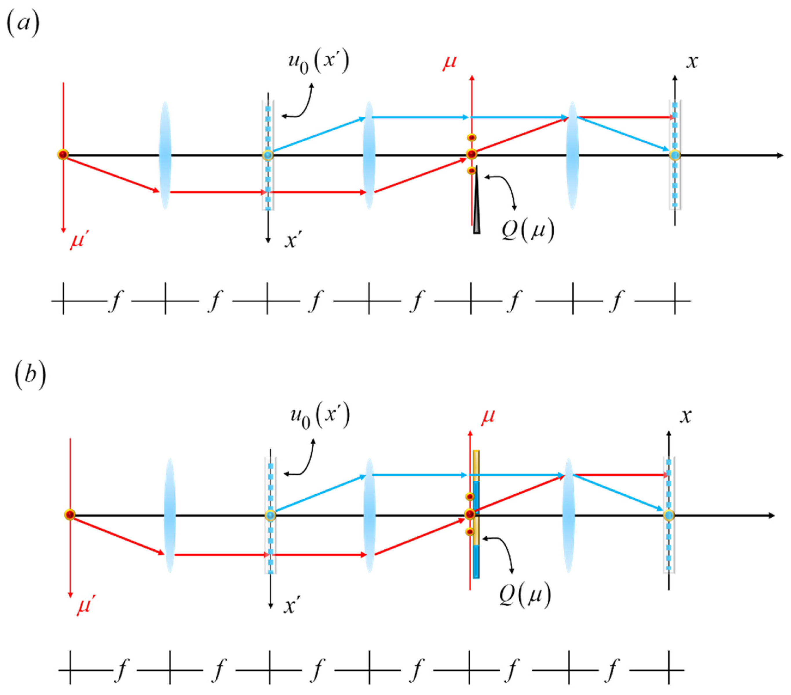
Figure 2.
Amplitude transmittance of the mask , as well as its even component and odd components. In (a) we depict the amplitude transmittance of the knife edge. In (b) we show its even component. In (c) we show its odd component. Next, the amplitude transmittance of the modulation contrast mask, as in reference [31]. In (d) we illustrate its amplitude transmittance. In (e) we show its even component. And in (c) we display its odd component.
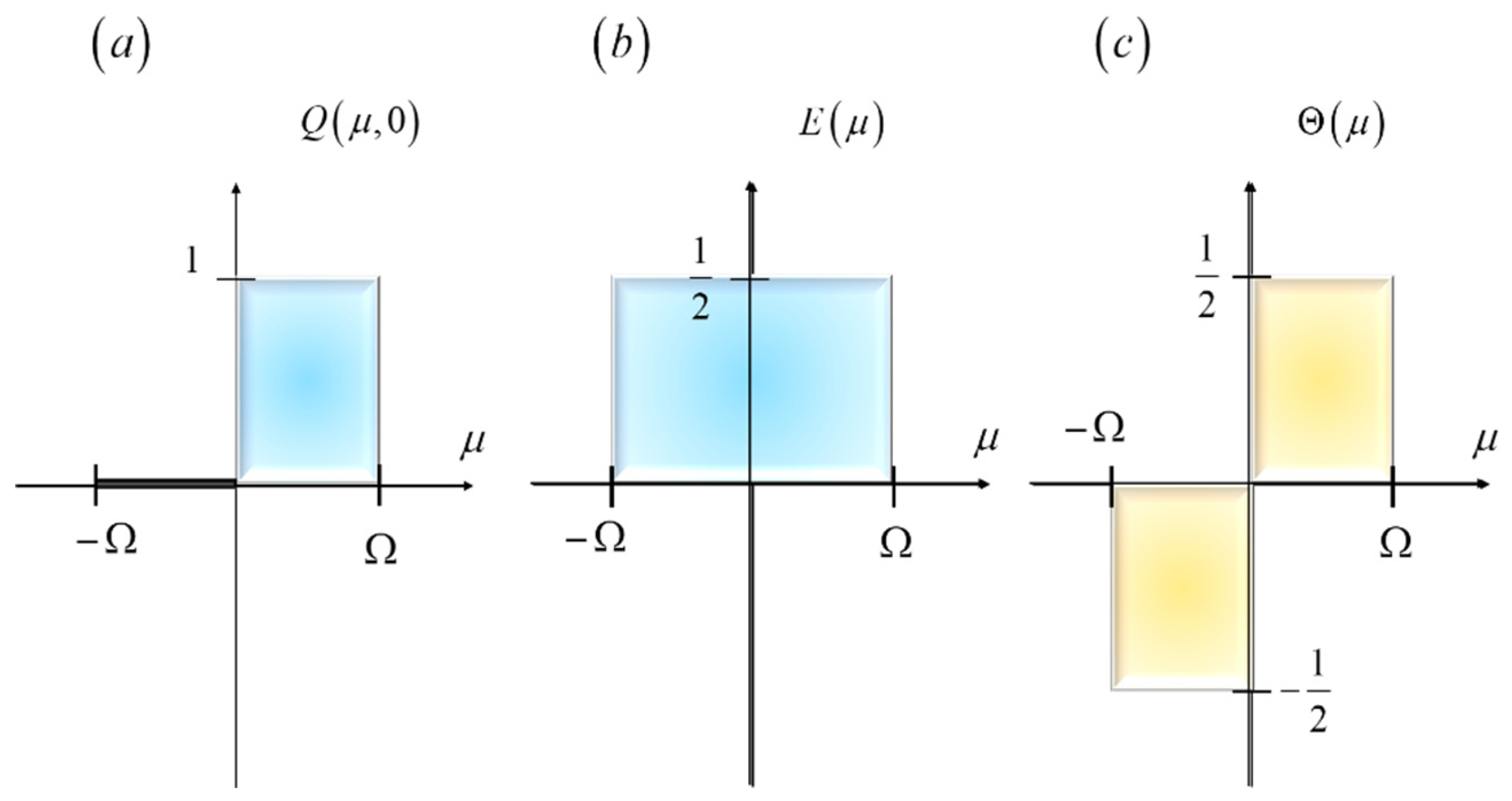
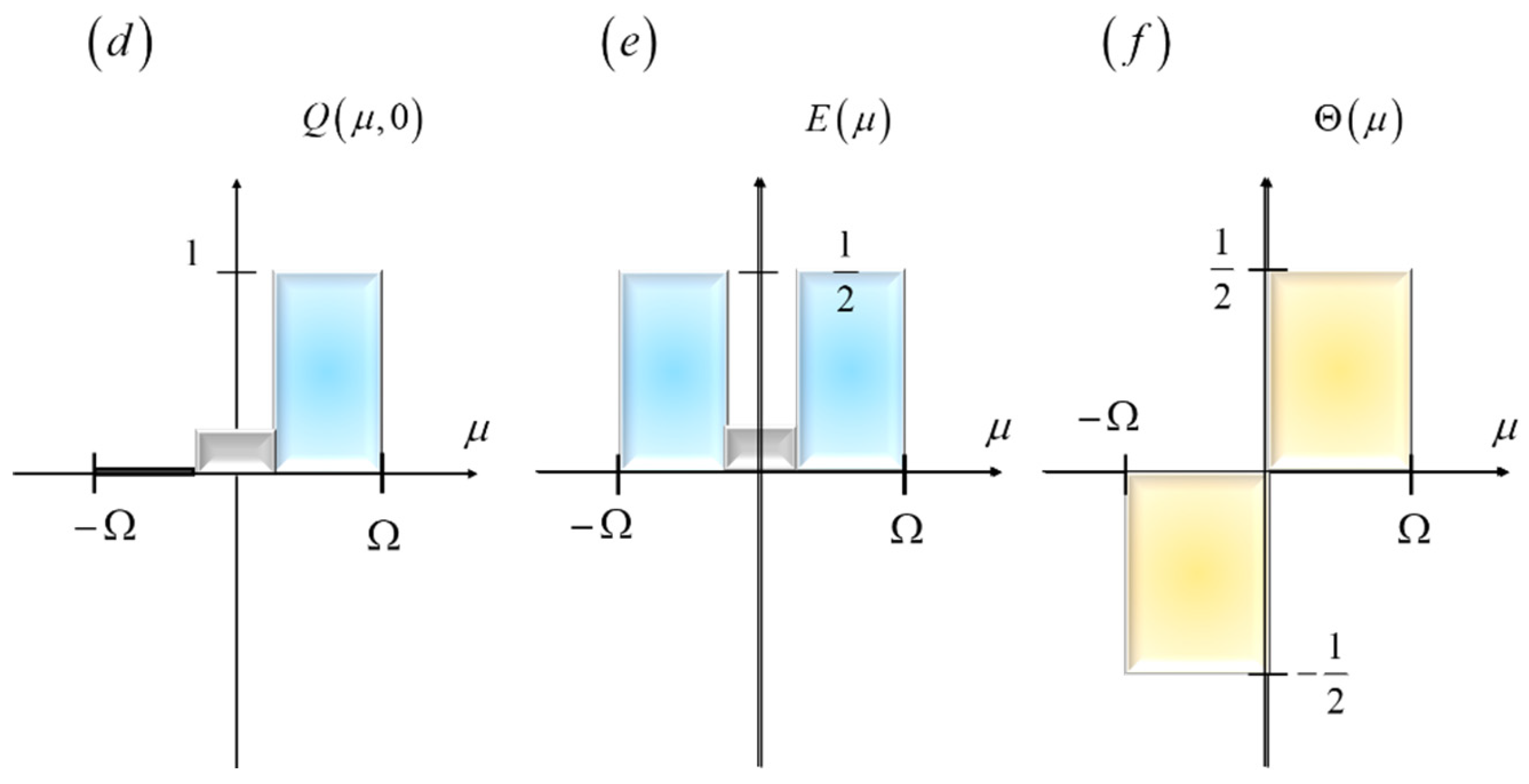
Figure 3.
Pictorial portraying the spatial frequency transfer of an initial amplitude sinusoidal distribution, into the final irradiance cosinusoidal distribution. At the center of the schematics, we depict the spatial frequency windows described in Equation (10).
Figure 3.
Pictorial portraying the spatial frequency transfer of an initial amplitude sinusoidal distribution, into the final irradiance cosinusoidal distribution. At the center of the schematics, we depict the spatial frequency windows described in Equation (10).
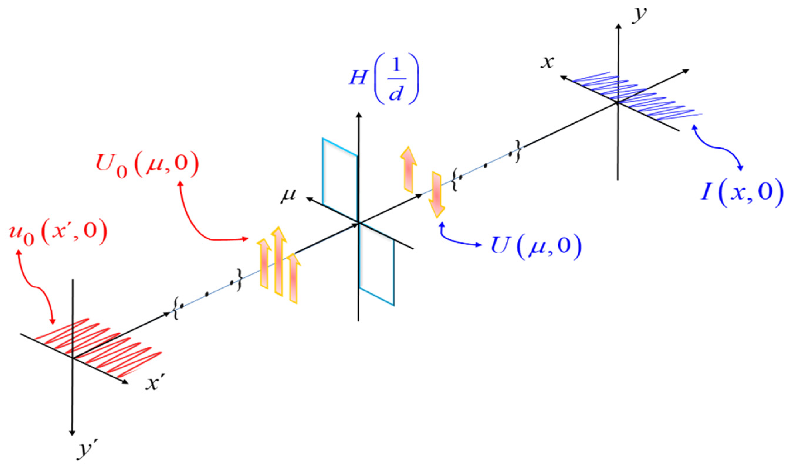
Figure 4.
Amplitude transmittance of an improved Schlieren technique. In (a) the amplitude distribution incorporates the light gathering advantage described in Equation (11). This mask also incorporates the advantage of reducing the amplitude transmittance, at the center of the mask, E(0), as in Equation (12). In (b) the odd component of the proposed mask.
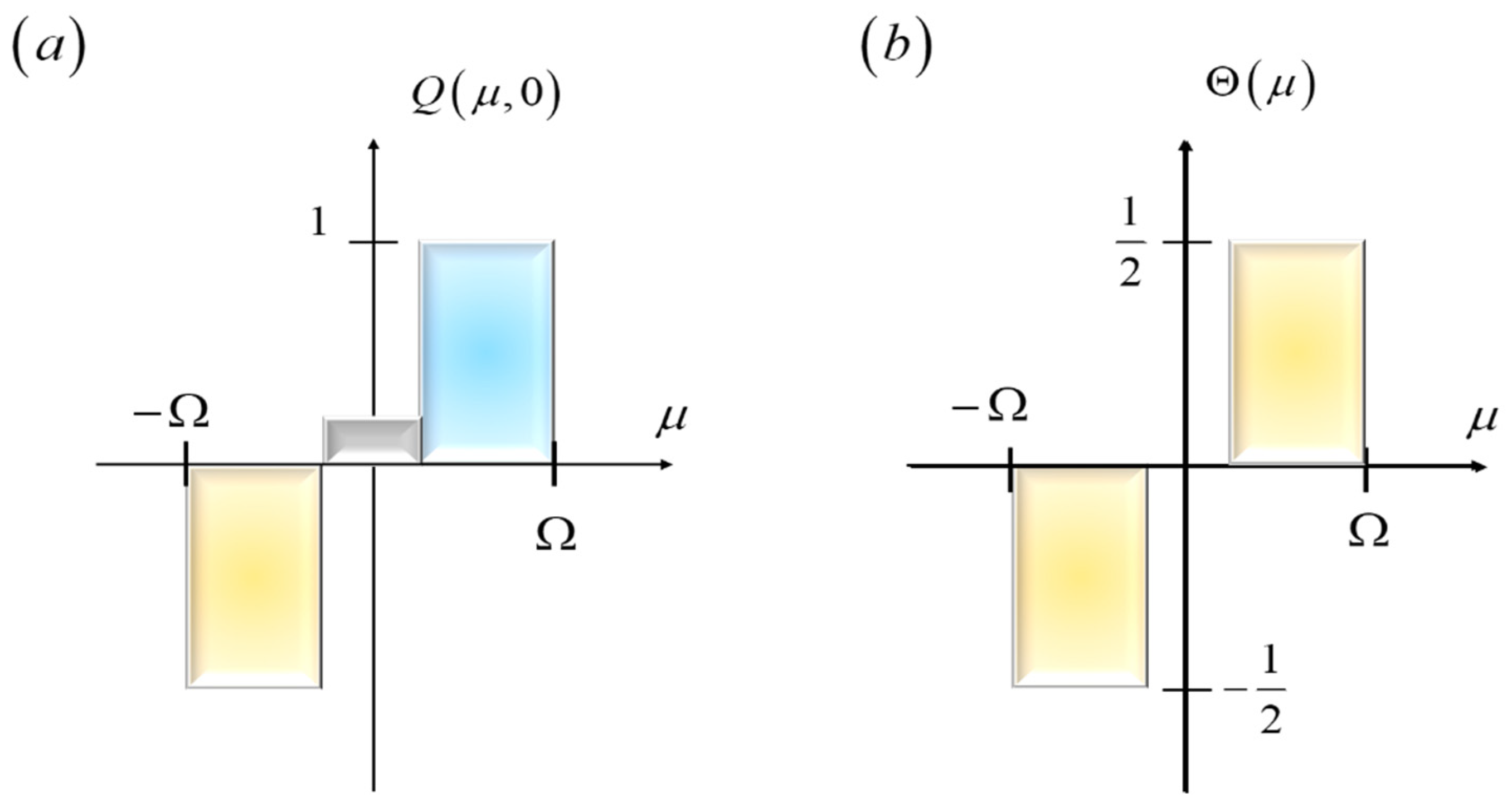
Figure 5.
Same as Figure 3, but now the effective transfer function is , as in Equation (20).
Figure 5.
Same as Figure 3, but now the effective transfer function is , as in Equation (20).
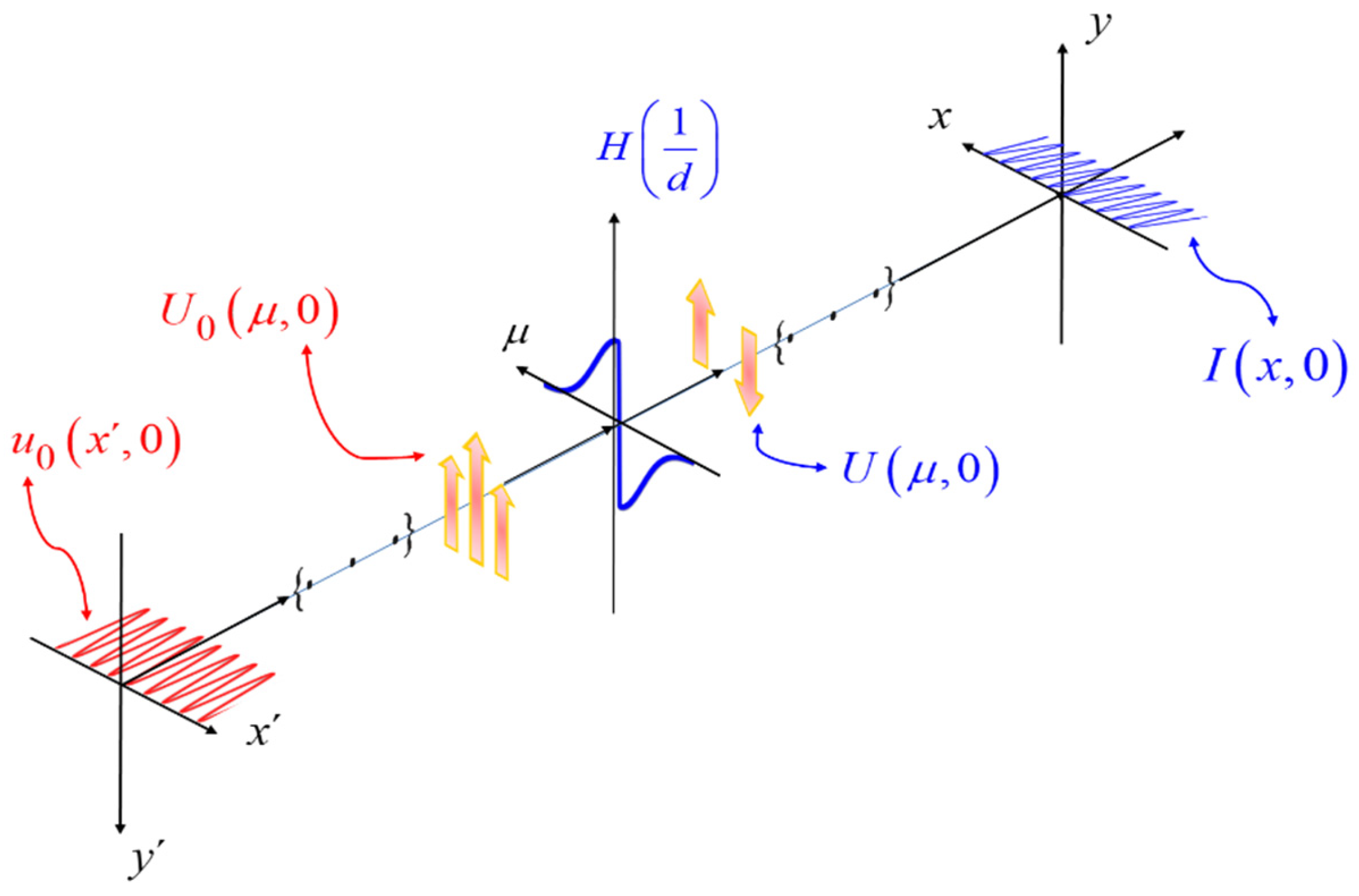
Figure 6.
The use of a coded source, in conjunction with a coded spatial filter. In (a) the source is a slit. At its conjugate image, the spatial filter is also a slit. In (b) we depict the impact of a phase gradient. In (c) two coded masks are used for implementing a mask product.
Figure 6.
The use of a coded source, in conjunction with a coded spatial filter. In (a) the source is a slit. At its conjugate image, the spatial filter is also a slit. In (b) we depict the impact of a phase gradient. In (c) two coded masks are used for implementing a mask product.
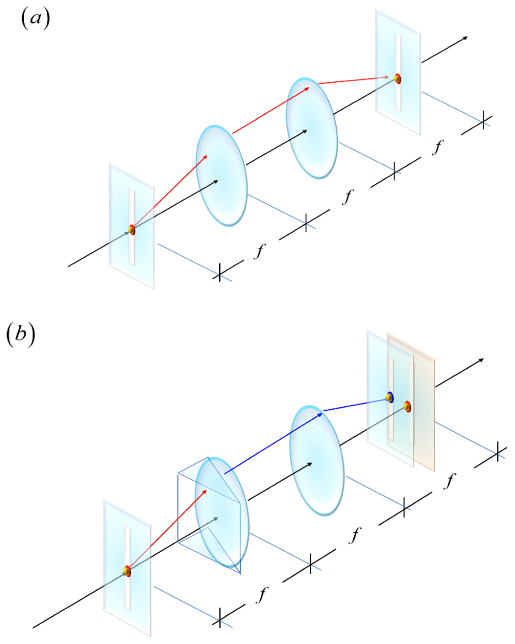
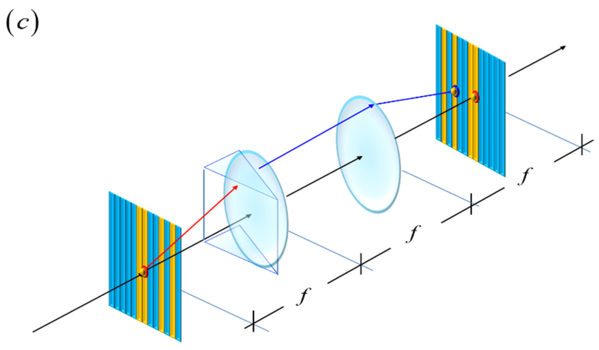
Figure 7.
Amplitude transmittance of the mask, Q L (η), which is coded with a pseudorandom sequence of length L. In (a) the length is L = 7. In (b) the length L = 15.
Figure 7.
Amplitude transmittance of the mask, Q L (η), which is coded with a pseudorandom sequence of length L. In (a) the length is L = 7. In (b) the length L = 15.
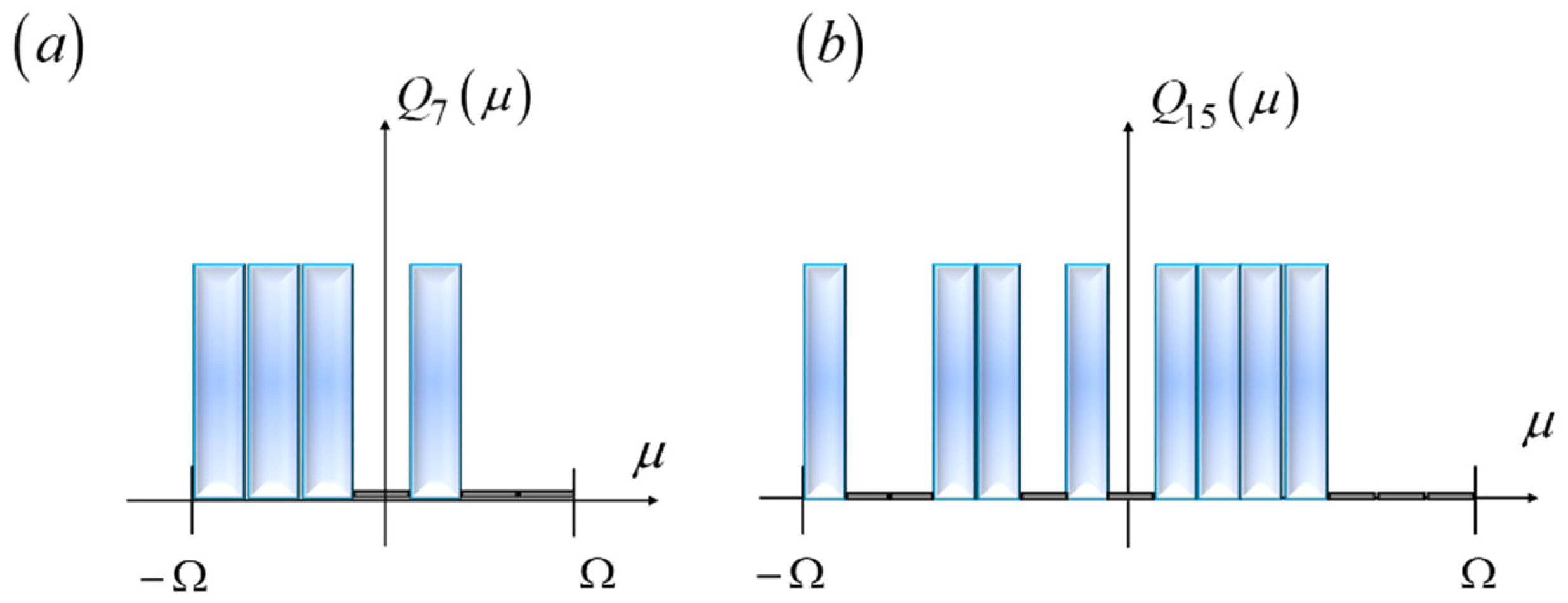
Figure 8.
Cyclic autocorrelations associate with the pseudorandom sequences in Figure 7. The cyclic autocorrelations exhibit peaks that overreach a uniform value.
Figure 8.
Cyclic autocorrelations associate with the pseudorandom sequences in Figure 7. The cyclic autocorrelations exhibit peaks that overreach a uniform value.
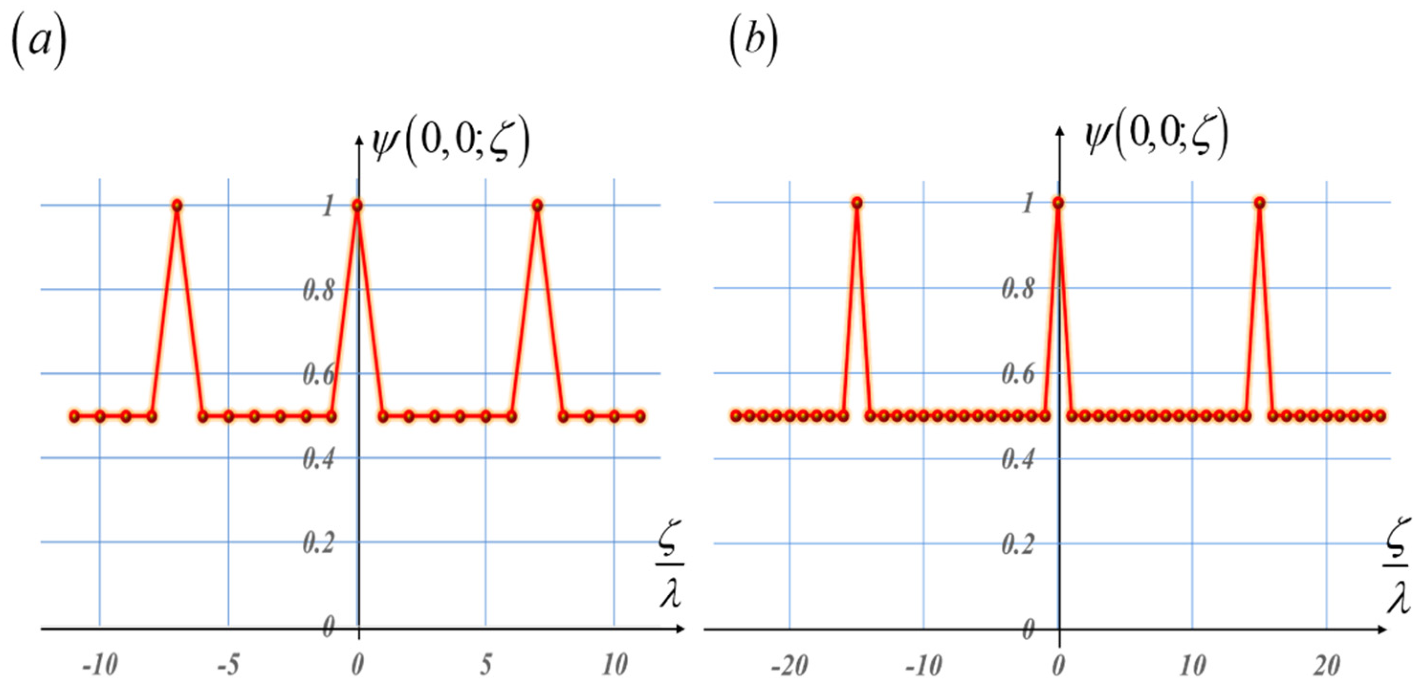
Figure 9.
Amplitude transmittance of the mask, Q L (η), which is coded with a Barker sequence of length L. In (a) the length is L = 7. In (b) the length L = 13.
Figure 9.
Amplitude transmittance of the mask, Q L (η), which is coded with a Barker sequence of length L. In (a) the length is L = 7. In (b) the length L = 13.
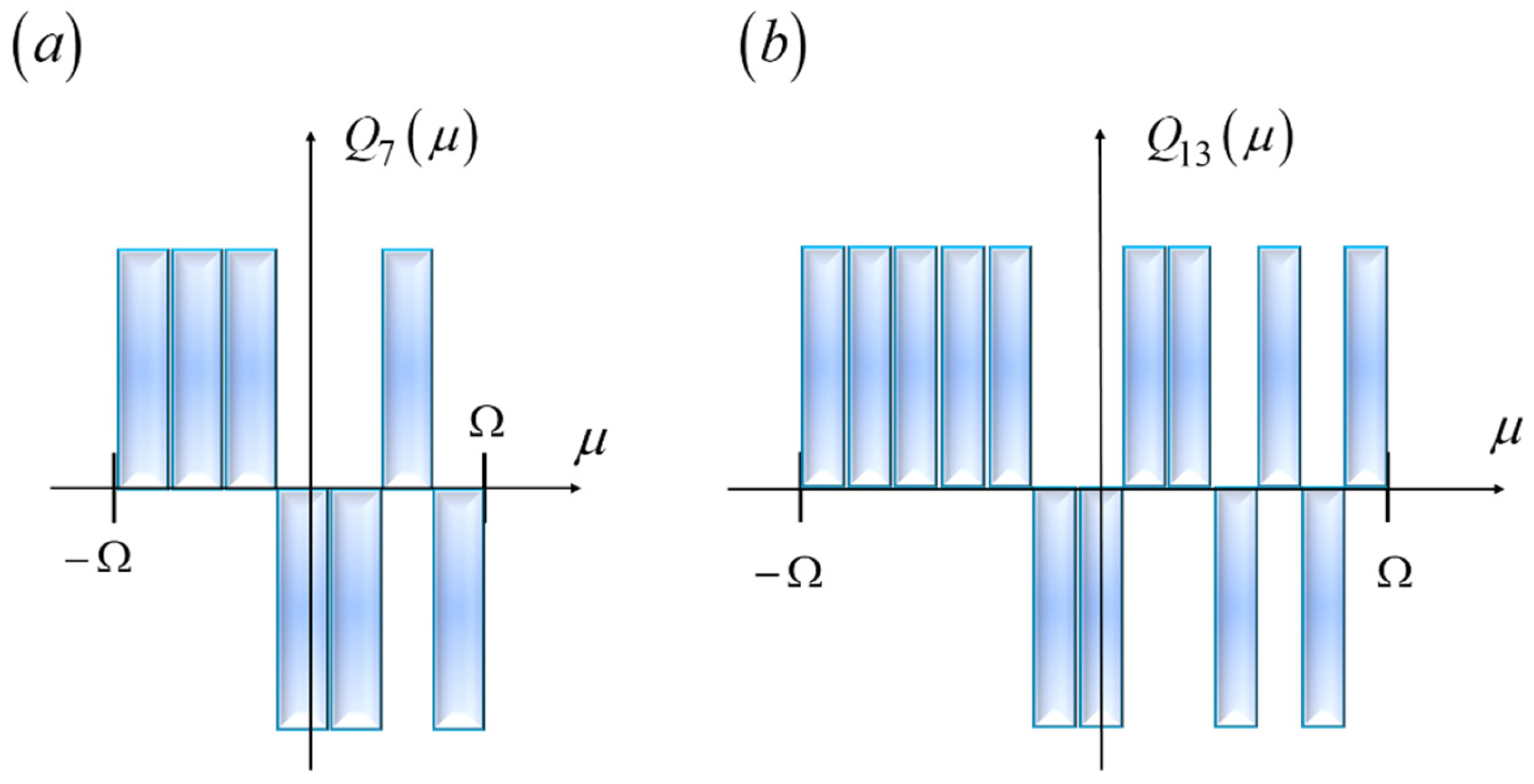
Figure 10.
Cyclic autocorrelation associated with the Barker sequences in Figure 9.
Figure 10.
Cyclic autocorrelation associated with the Barker sequences in Figure 9.
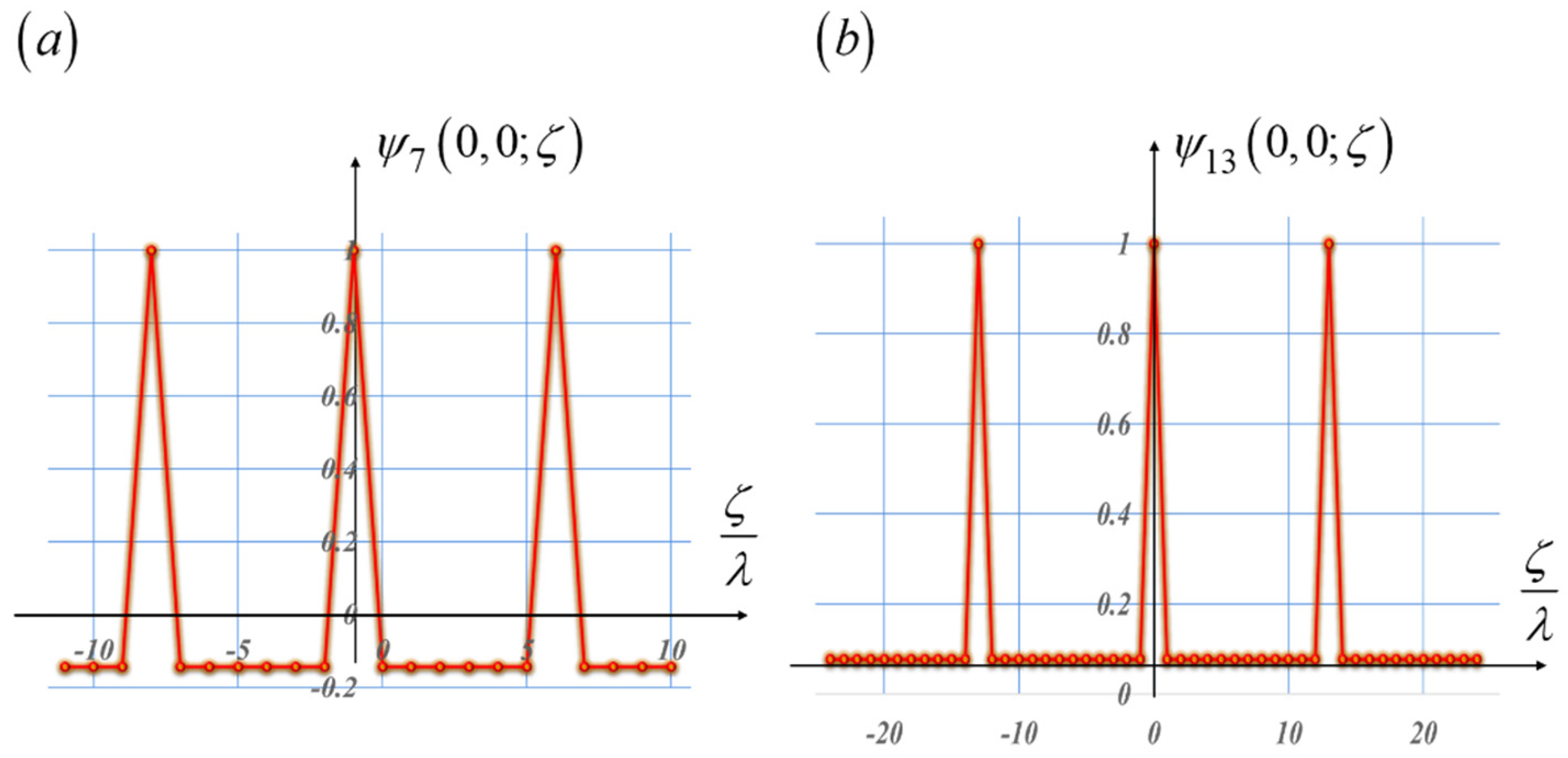
Figure 11.
Like Figure 7. However, autocorrelations are noncyclic. Now, the pseudo random sequences have values of unity or minus unity. The noncyclic autocorrelations have a distinctives central peak, with nonuniform sidelobes.
Figure 11.
Like Figure 7. However, autocorrelations are noncyclic. Now, the pseudo random sequences have values of unity or minus unity. The noncyclic autocorrelations have a distinctives central peak, with nonuniform sidelobes.
Figure 12.
Like Figure 10. However, now the autocorrelations are noncyclic. They exhibit a single central peak, with sidelobes that have constant value.
Figure 12.
Like Figure 10. However, now the autocorrelations are noncyclic. They exhibit a single central peak, with sidelobes that have constant value.
Figure 13.
Schematics of a Schlieren technique that acts as an automatic sensor of phase gradients. In (a) an unfolded version. In (b) a folded version.
Figure 13.
Schematics of a Schlieren technique that acts as an automatic sensor of phase gradients. In (a) an unfolded version. In (b) a folded version.
Disclaimer/Publisher’s Note: The statements, opinions and data contained in all publications are solely those of the individual author(s) and contributor(s) and not of MDPI and/or the editor(s). MDPI and/or the editor(s) disclaim responsibility for any injury to people or property resulting from any ideas, methods, instructions or products referred to in the content. |
© 2025 by the authors. Licensee MDPI, Basel, Switzerland. This article is an open access article distributed under the terms and conditions of the Creative Commons Attribution (CC BY) license (http://creativecommons.org/licenses/by/4.0/).
Copyright: This open access article is published under a Creative Commons CC BY 4.0 license, which permit the free download, distribution, and reuse, provided that the author and preprint are cited in any reuse.


