
Submitted:
19 April 2025
Posted:
21 April 2025
You are already at the latest version
Abstract
This paper proposes a novel approach to modeling the dependence of the number of cycles to failure on the initial crack length and stress amplitude. This model is applicable in the context of linear fracture mechanics in polycrystal materials, particularly metal alloys. The principal benefit of the proposed functions is that they enable the potential for obtaining closed-form analytical solutions for the fractal crack growth law. This proposed fractal propagation function is based on the hypothesis that the load ratio stays the same throughout the load history, and it describes the small in-crease in crack length with each cycle. In contrast to the common propagation laws, the crack length growth depends on branching of the crack. This feature enables a straightforward representation of the transition from common, straight cracks to fractionally non-planar cracks in metals. We pro-pose two fractional spreading functions, each with a different number of fitting parameters. One advantage of the proposed closed-form analytical solutions is that they facilitate the universal fit-ting of the constants of the fatigue law across all stages of fatigue. Another advantage is that the closed-form solution simplifies the application of the fatigue law, as the solution of a nonlinear fractional differential equation is no longer necessary. In addition, the corresponding formulas for the length of the non-fractional crack over the number of cycles are derived in terms of Lerch functions.
Keywords:
fractional Paris-Erdogan law
; linear fracture mechanics
; fractional derivative
Contents
- The growth of fractal crack 2
- The laws of propagation for cyclic loads 4
- Equation of the Fractal Crack (type I) 6
- Equation of the Fractal Crack (type II) 9
- Threshold-bounded formulations for propagating functions 10
- Conclusion 12
- List of symbols 13
- References 14
1. The Growth of Fractal Crack
The functional relationship between the loading properties, stress gradient, and the physical time-dependent characteristics of materials is fundamental to statistical fatigue analysis and the subsequent calculation of the number of cycles to failure (Carpinteri, 1994), (Suresh, 1998); (Fatemi & Yang, 1998), (Tada, Paris, & Irwin, 2000).
The process of fatigue fracture in metals can be categorized into three distinct stages: initiation, propagation, and final rupture (Totten, 2008), (Leese & Socie, 1989).
In the initial phase of fatigue in elastic polycrystal media, the initiation stage (Stage I) is characterized by the observation of a deceleration in the propagation of the fatigue crack with increasing cycle number, indicating the onset of the second stage of the process. This subsequent stage, referred to as crack propagation (Stage II), involves the propagation of the fatigue crack in a smooth and consistent manner. During this stage, the microscopic crack undergoes a change in direction, growing perpendicular to the tensile stress. The propagation stage is the most readily identifiable phase of a fatigue fracture.
The Paris law, as described by (Paris & Erdogan, 1963), provides a mathematical model for stage II propagation. This model posits the propagation of a fatigue crack per unit cycle as a power function of the range of the stress intensity factor.
The mechanical fatigue limit of vulcanised rubbers can be accurately predicted using the critical energy approach. The characteristics of cut growth at low crack energies and the effects of physical parameters on the critical crack energy and fatigue limit have been discussed by (Lake & Lindley, 1965). The actual paper looks exclusively at the study of fatigue phenomena in polycrystalline materials, focusing on metal alloys. However, it is recognised that the methodology presented in this study can also be applied to plastic and amorphous materials, such as rubber.
Since the 1970s, many models for predicting damage to structures have been created. These models build on the manuscript (Paris & Erdogan, 1963). The idea that the common propagation law can be slightly different at the threshold was first suggested by (Donahue, Clark, Atanmo, Kumble, & McEvily, 1972). This law successfully explained a well-known phenomenon: the rapid growth of cracks that eventually cause tearing. The article gave an equation to fix the problem of brittle fracture based on the power law. In the study (Kanninen & Popelar, 1985) researchers investigated various combinations of high and low stress intensity factor values. Another study, (McEvily & Groeger, 1977), suggested a similar approach for the transition zone between high and low stress intensity factors.
In order to achieve an accurate depiction of failure at elevated numbers of cycles, the structural materials are to be subdivided into two distinct categories: Type I and Type II (Mughrabi, 2006). The distinguishing characteristics of these materials include their purity, single-phase composition, annealed state, ductility, and the absence of significant internal defects.
A more generalized "unified law" has been proposed which accounts for certain deviations from the power-law regime (Pugno, Cornetti, & Carpinteri, 2007). The extension of the Paris law for crack propagation results in the generation of generalized Wöhler fatigue curves.
The transition region from high to low stress amplitudes is identified at a specific point (Abe, Furuya, & Matsuoka, 2001). t.The fatigue life curves display a near-piecewise-linear character with a distinct corner point in logarithmic scaling.The concept of endurance strength was identified as an endurance threshold limit for the stress intensity factor.
According to (Newman, 1984), the note posits a general crack opening stress equation for constant amplitude loading. The equation assumes an elongation per cycle as the expression, which depends on a stress ratio, stress level, and certain three-dimensional constraints describing the shape of the crack. The effects of these three-dimensional constraints have been simulated in a two-dimensional closure model by using a factor for tensile yielding.
The pioneering work reviewed the use of fractal structure to describe microstructural features of metals (Mandelbrot, Passoja, & Paullay, 1984). Hornbogen's review expanded the characterization technique for fracture surfaces by incorporating fractal theory concepts (Hornbogen, 1989), (Skrotzki & Hornbogen, 1994). The fractal structure was expanded relating a multitude of parameters, including the distribution of phases (Mecholsky, Passoja, & Feinberg-Ringel, 1989), martensitic and dendritic configuration (Mu & Lung, 1988), dislocation arrays (Tanaka, 1996), slip bands (Tsai & Mecholsky Jr, 1991), grain boundaries (Xin, Hsia, & Lange, 1995), and fracture surface roughness (Nagahama, 1994), (Lung, 1986).
A considerable body of literature has investigated the relationship between the fractal dimension of a fracture surface and the experimental values of the corresponding fracture toughness (Rodrigues & Pandolfelli, 1998). The recurrently reported properties and features in these studies include impact energy, fracture toughness, the type of fracture along the crack propagation, and roughness.
In the study (Maierhofer, Pippan, & Gänser, 2014), an analytical model was developed to describe how fast short and long cracks can grow under certain conditions. This model was used to study how residual stresses affect crack growth behavior. This investigation allowed us to understand how the combined effects of load and residual stresses, along with the build-up of crack closure, influence fatigue crack growth. As a result, a simple yet effective change to a formula used to predict how fast cracks grow was suggested. This approach was checked by doing experiments, and it was discussed how it could be used to see if surface-treated parts are fit for their purpose.
A fractography analysis was conducted in (Wojciech Macek, Faszynka, Branco, Zhu, & Nejad, 2023) for 2017-T4 aluminum alloy subjected to cyclic bending. A comparative analysis of fracture surface features was carried out using standard surface topography parameters and non-standard surface topography parameters , including fractal dimension Df. The introduction of a damage parameter that integrates both fractographic characteristics and stress state information was instrumental in assessing the fatigue durability of the material.
The objective of this paper is to provide a concise rederivation of one of the formulas derived in the aforementioned article (Kobelev, A proposal for unification of fatigue crack growth law, 2017). The paper presents a novel investigation into the dependencies of cycles to failure for a given initial crack length upon stress amplitude in the linear fracture approach.
The paper (Kobelev, Forman–Kearney–Engle fractal propagation law of fatigue crack, 2025) presents a closed-form analytical expression for the Forman–-Kearney–-Engle fractional-differential relationship between crack length and the number of cycles. Two novel functions have been introduced to express the damage growth per cycle. These functions facilitate the unification of disparate fatigue laws within a single expression, thereby providing a unified framework for analysis. The unified fatigue law provides analytical solutions for the relationship between crack length and the mean value and range of cyclic variation of the stress intensity factor. The solution presents the number of cycles to failure as a function of the initial size of the crack. This eliminates the need to solve a nonlinear fractional differential equation of the first order. The explicit formulas for stress versus number of cycles to failure are provided for both proposed unified fatigue laws.
The present manuscript proposes a substantial augmentation to a previously established methodology by incorporating fractional-differential relations. This incorporation facilitates the inclusion of an additional free parameter, thereby enabling the precise representation of experimental data. The principal difference between the actual research and the research (Kobelev, Forman–Kearney–Engle fractal propagation law of fatigue crack, 2025) is the following. The aforementioned hypothesis is predicated on the premise that there is a reduction in the propagation rate of cracks in the region of short crack length and low stress amplitude. In contrast, the Forman–Kearney–Engle propagation formula is employed to calculate the fracture toughness, which is defined as a material constant. It has been determined that this constant is independent of crack length; that is to say, it remains constant for any given crack length. Moreover, it has been ascertained that the critical value of the applied tension stress corresponding to every half crack length in an infinite sheet is determined by this constant. The formula for crack length over the number of cycles is finally derived using Lerch functions.
2. The Laws of Propagation for Cyclic Loads
2.1. The subsequent section will examine the laws of propagation in relation to cyclic loads. Crack propagation will be calculated as a function of the range of the stress intensity factor:
.
The factors in this equation are as follows:
the maximum stress intensity factor and
the minimum stress intensity factor per cycle.
Paris' law is a common form of quantification that is employed to determine the fatigue life of a specimen for a given crack size, . The range of stress intensity factor is as follows:
.
The range of stress intensity factor is contingent on:
the stress range,
the maximum stress,
the minimum stress per cycle,
the mean stress in cycle,
a dimensionless parameter that reflects the geometry.
The parameter possesses the value 1 for a center crack in an infinite sheet. In the present paper the traditional form for propagation law is implemented:
The propagation function is defined as the infinitesimal increase in crack length per unit increase in the number of load cycles n. The load ratio remains constant over the load history.
The symbol in Eq. (1) indicates the ordinary derivative of the function :
.
Subsequently, the demonstration shall be presented that the solution to Equation (1), which incorporates fractional derivatives, can be achieved by means of interchanging the independent and dependent variables. The ordinary derivative of corresponding inverse function reads:
.
The coefficients in the Eq. (1) are:
the material constant for a given stress ratio ,
the stress ratio of cyclic load,
the mean value of stress intensity factor.
It is possible to account for the variations in range and the mean value of the stress intensity factor over the load history by applying theories on damage accumulation (Sorensen, 1969) and (Wheeler, 1972).
The following equation describes the growth of the crack length with an increasing number of cycles , or equivalently where (Paris & Erdogan, 1963):
The material exhibits initial cracks, characterised by their length, designated as , The cycle count commences at the onset of crack propagation from its initial length:
2.2. As demonstrated in the aforementioned literature, extensive experimental evidence indicates that the S-N curves can be represented as nearly piecewise-linear graphs.This phenomenon can be explained from the perspective of crack propagation. In the initial stage, an examination of the planar crack with two distinct propagation regimes is undertaken.The growth of cracks occurs in a direction that attempts to maximize the subsequent energy release rate and minimize the strain energy density. The propagation path that optimizes this objective is aligned with the direction of maximum extension strains. Accordingly, the shape of the crack should be an ideally straight line. As the crack grows, the process of crack extension accelerates, resulting in a higher rate of elongation of the crack length per cycle, denoted as
. The crack gains sufficient strength to deform the polycrystalline material at its tip, thereby facilitating the most direct path for its propagation across the grain regions. The two processes occur concurrently, but the proclivity for grain destruction is dominant in the presence of elevated stresses.
It is assumed that the planar crack propagation would occur in the direction of greatest energy efficiency. Consequently, in the event of homogeneous material, the crack will propagate in the direction that is energetically optimal. This direction results in the greatest possible elongation for the given direction of the greatest principal stress. In the second step, we put forward a mechanism for crack extension that accounts for the deviation of the crack from its energetically preferred direction. The following consideration is proposed. It is evident that the process of fracture is an anisotropic phenomenon. The growth of microcracks occurs in directions that attempt to maximise the energy release rate and minimise the strain energy density. The process of crack propagation along grain boundaries necessitates a lesser expenditure of energy in comparison to the process of crack propagation across perfect grain crystals. The orientation of grain boundaries is randomly distributed. Therefore, the optimal propagation path deviates randomly from the ideal straight path, which is normal to the maximum principal stress. Furthermore, the deviation is attributable to the disordered orientations of anisotropy in grains and the highly warped grain boundaries. Therefore, due to the arbitrary anisotropy of individual polycrystalline domains and their irregular shapes, the crack does not follow a straight direction and randomly deviates from the direction that would be most energetically favourable. These considerations are employed in the construction of the physical background of the proposed mathematical model.
3. Equation of the Fractal Crack (Type I)
3.1. The first form of the equation, which describes how the crack propagates in the fractal medium, is as follows. This formulation assumes the application of the fractional differentiation operator
to the left side of equation (1):
The symbol in Eq. (3) indicates the sum of the ordinary derivative and fractional derivative of the order of the function :
The method is used to calculate the fractional derivative using the definition (Davison & and Essex, 1998), that is, first differentiate times, then integrate times:
where smallest integer greater than or equal to a number , . This definition handles differentiation orders .
The unit of the ordinary derivative is The unit of the fractional derivative of the order is The symbol represents the characteristic transition length between the fractal and common regimes. The factor has a unit of . Consequently, the unit of the derivative is The parameter is defined as a material property that is contingent upon the material's chemical composition and the specific heat treatment it undergoes. The characteristic value of this parameter is indicative of the size of the crystal grain in the polycrystal alloy. The dimensionless parameter is employed for the purpose of norming the equation. The value corresponds the ordinary differential equation in form of (Paris & Erdogan, 1963). The value leads to the fractional differential equation. For further presentation the value will be used.
The stress intensity factor that corresponds to the transition between the fractal and common regimes is .
3.2. It is initially presumed that
. The common propagation law (2), the crack length growth pro cycle depends solely on the stress intensity factor. In the proposed law, the crack length growth is contingent on the branching of the crack. This facilitates the straightforward representation of the transition from a common straight crack to a fractionally non-planar crack. The factor λ is a critical metric in the crack length, as it is instrumental in delineating the transition from the planar crack propagation to the branching regime. The employment of the fractional derivative in place of the conventional derivative within equation (3) results in the formulation of an integral-differential equation:
For the sake of brevity, we will henceforth use in our formulas the auxiliary value:
.
The integral transformation method is a valuable tool for solving linear fractional differential equation (6) (Luchko, 2019). The application of the Laplace transform to equation (6) results in the following linear algebraic equation:
The Laplace transform of the function is the unknown in the equation (7). The initial condition reads:. The solution of the equation (7) delivers the transformed function:
The Bromwich integral inverse Laplace transform of the function (8) is the solution to the fractional differential equation (6). The solution could be obtained with the common methods (Luchko, 2019). In order to identify the most elementary expression for closed-form solutions, it is necessary to establish the value of the fractional derivative , :
The number of cycles required for a crack to grow from a length of to a length of is given by the following expression:
One particular scenario, corresponding to the parameter , is that the crack progresses from start to finish in a fractal pattern:
The application of the Laplace transforms to the Eq. (11) and leads with to the transformed function
The inverse Laplace transform of (12) provides the closed form expression. In case , the number of cycles required for the crack to grow from length to length is equal to:
The other limit case corresponds to the parameter. This case corresponds to a common linear fracture mechanics due to (Paris & Erdogan, 1963). The crack progresses from start to finish in a linear trajectory:
The number of cycles necessary for crack growth from length to length reads:
3.3. Secondly, it is presumed that
. The definition of the fractional derivative, as delineated in equation (3), gives rise to an integral-differential equation:
The integration of the transformation method is employed once more in order to arrive at the solution to the linear fractional differential equation (16),(Luchko, 2019). The subsequent linear algebraic equation is derived from the implementation of the Laplace transform on the given equation (16):
Equation (17) contains the Laplace transform of the function as an unknown. The initial conditions require two constants:
The solution of the equation (17) delivers the transformed function:
For closed form solutions the value of fractional derivative will be put ,and the initial conditions assume . The solution to the fractional differential equation (16) is derived from the application of the Bromwich integral inverse Laplace transform of the function (19). The solution reads:
The quantity of cycles required for the crack to extend from a length to a length is equivalent to the following expression::
It is important to note that one limit case corresponds to the parameter θ being equal to zero . In this particular instance, the crack exhibits a fractal pattern of propagation, extending from its origin to its terminus within the fractal medium:
The application of the Laplace transforms to equation (23) and the subsequent integration of the resulting function leads to the following result, given the conditions :
The inverse Laplace transform of equation (24) affords a closed-form expression. In case , the number of cycles required for the crack to grow from length to length is equal to:
The other limit case corresponds to the parameter , as demonstrated in Equations (14) and (15). Henceforth, for the purpose of plotting, the value is assumed to be:
4. Equation of the Fractal Crack (Type II)
4.1. The second formulation presupposes the implementation of the fractional differentiation operator, denoted , on the right-hand side of the Eq. (1):
According to equation (26), the definition of the fractional derivative leads to an ordinary inhomogeneous differential equation of the first order:
The application of the Laplace transform (29) yields the following expression:
4.2. The number of cycles can be found by using the inverse Laplace transformation of the expression (30). Particularly, we get for :
The subsequent expression provides the number of cycles necessary for a crack to extend from a length to a length :
In the event that , the fully-fractional limit case manifests itself as follows:.
The other limit case, denoted by , corresponds to an infinitesimally small scaling parameter, λ. This leads to the equation (14) with an already known solution (15):
.
4.3. For , the inverse Laplace transformation of the expression (29) results in the formula for the number of cycles:
The number of cycles required for a crack to grow from length to length is given by the following expression:
The fully-fractional limit case follows from the equations (35), (36) with :
The other limit case, , corresponds to an infinitesimally small scaling parameter, . It yields the equation (14) with a known solution (15).
5. Threshold-Bounded Formulations for Propagating Functions
5.1. For a specific set of alloys, a theoretical value for stress amplitude exists. According to this theoretical framework, the material will not fail for any number of cycles if the stress amplitude remains below this theoretical value.
This paper employs a method of representing crack propagation functions through appropriate elementary functions. The choice of elementary functions is motivated by the available phenomenological data and covers a broad range of possible parameters. The crack propagation functions that have been introduced allow for the rigorous solution of differential equations that describe the crack propagation. The resulting closed-form solutions facilitate the evaluation of crack propagation histories and the effects of stress ratio on crack propagation.
The report (Miller & Gallagher, 1981) presents eight different methods for predicting fatigue life. Each of the presented methods can be applied to describe the three regions of the crack growth rate curve. The propagation function for damage growths per cycle encompasses the Paris propagation law and transition regions at elevated and diminished levels of stress intensity factors:
is the exponent at the short-term limit ,
is the endurance limit exponent .
The values , , and are material properties. The objective of this section is to determine the compact form of closed-form solution of the ordinary differential equation (39) with the initial condition:
The function shows the number of times the crack length grows from the starting value to the given value . This is true as long as the stress range and mean stress stay the same. Using equation (39), we can find two ultimate crack sizes right away. First, the value is the critical crack length at which instantaneous fracture will occur:
Secondly, the following value indicates the first crack length that causes fatigue cracks to start growing:
This estimation is based on the given stress range.
If the following condition is met
the initial crack length breaks after a certain number of cycles. The number of cycles will be explained in more detail below.
The unified propagation function (39) due to (Miller & Gallagher, 1981) could be studied in closed form, as shown later.
5.2. The Figure 6 shows how the crack growth rate
and the range of stress intensity factor () are related for the materials that were simulated. The endurance and short-time threshold exponents were measured in experiments (Albrecht, Martin, Lüthering, & Martin, 1976), aluminum alloys X-7075 (180°), X-7075 (100°), 7075 (100°).
The solution to the ordinary differential equation (41), given the initial condition, can be expressed in a simple analytical formula. This new formula gives the number of cycles left to break down:
The auxiliary function in Eq. (42) reads:
The Lerch -transcendent from (Lerch, 1887-1888), or §1.11, (Bateman & Erdelyi, 1953) appears In Eq. (43):
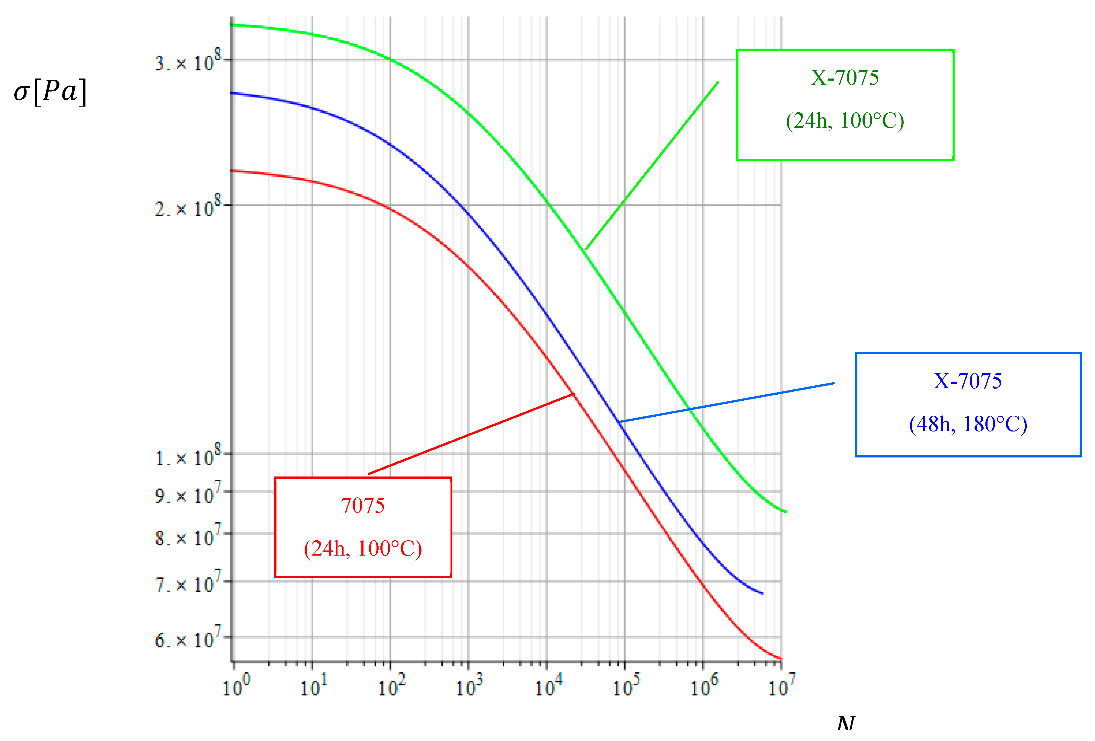
The following example shows how the metallic material with the unified propagation function (39) acts. The resulting diagrams show how cycles to failure (S-N curves) for aluminum alloys X-7075 (180°), X-7075 (100°), and 7075 (100°) (Albrecht, Martin, Lüthering, & Martin, 1976) look. The diagrams for are presented on the pictures on Figure 7. We used the same initial crack length (in all cases to be sure. The stress intervals for the calculations are contingent upon the threshold stress intensity factor:
As illustrated in the subsequent images, the correlation between crack length and cycle duration is depicted by the a-N curves. The numerical value of cycles is determined by the length of the crack within the specified interval:
6. Conclusion
The length of the crack's growth is contingent upon its branching structure, a phenomenon that diverges from the conventional framework employed in the description of propagation laws. This method is effective in demonstrating the transition of a straight crack into a non-planar crack. The manuscript is founded upon a preceding methodology incorporating fractional differential relations, which permits the incorporation of an additional free parameter to facilitate the precise representation of experimental data.
The objective of this paper is to propose a novel approach to modeling the dependence of the number of cycles to failure on the initial crack length and stress amplitude in the context of linear fracture mechanics in polycrystal materials, particularly metal alloys.The principal benefit of the proposed functions is the potential for obtaining closed-form analytical solutions for the fractal crack growth law. The proposed fractal propagation function is predicated on the assumption that the load ratio remains constant over the load history, and it describes the infinitesimal crack length growth per increasing number of load cycles. In contrast to the conventional propagation laws, the crack length growth is contingent on the branching of the crack. This enables a straightforward representation of the transition from a common straight crack to a fractionally non-planar crack in metals. Two fractional spreading functions, each with a different number of fitting parameters, are put forth for consideration.On the one hand, the closed-form analytical solutions facilitate the universal fitting of the constants of the fatigue law across all stages of fatigue.On the other hand, the closed-form solution simplifies the application of the fatigue law, as the solution of a nonlinear fractional differential equation is no longer necessary.
Furthermore, the corresponding formulas for the length of the non-fractional crack over the number of cycles are derived in terms of Lerch function. The paper presents an analytical expression for the relationship between the number of cycles and crack length in different fractal regimes. The fractional fatigue law provides analytical solutions for the relationship between crack length and the mean value and range of cyclic variation of the stress intensity factor. It introduces two novel functions that express the damage growth per cycle of the fractal crack. These functions facilitate the unification of disparate fatigue laws within a single expression, thereby providing a unified framework for analysis of variable elongation patterns. The solution shows the number of cycles to failure as a function of the initial size of the crack. Therefore, it can be concluded that the numerical solution of a nonlinear fractional differential equation of variable order is not a prerequisite for qualitative analysis.
Funding
This research received no external funding.
Institutional Review Board Statement
Not applicable.
Informed Consent Statement
Not applicable.
Data Availability Statement
The numerical results presented in this document can be replicated using the methodology and formulations described here. The analytical expressions used in the examples are available upon request to the authors.
Conflicts of Interest
The authors declare no conflicts of interest.
List of Symbols
| maximum stress intensity factor per cycle | |
| minimum stress intensity factor per cycle | |
| range of stress intensity factor, . | |
| stress range, | |
| maximum stress per cycle | |
| minimum stress per cycle | |
| dimensionless geometry parameter | |
| material constant | |
| Auxiliary parameter | |
| stress ratio of cyclic load | |
| mean value of stress intensity factor, | |
| unified propagation function of type I, Eq. (2) | |
| unified propagation function of type II, Eq. /(17) | |
| unified propagation function of type III, Eq. (25) | |
| fatigue exponent | |
| exponent at short-term limit | |
| endurance limit exponent | |
| short-term threshold limit () | |
| endurance threshold limit () | |
| number of cycles for growth of crack length | |
| . | Lerch transcendent, §1.11, (Bateman & Erdelyi, 1953) |
| Gamma function, §1.1, (Bateman & Erdelyi, 1953) | |
References
- Abe, T.; Furuya, F.; Matsuoka, S. Giga-cycle fatigue properties for 1800 MPa-class spring steels. Transactions of the Japan Society of Mechanical Engineers Vol.67, No.664 2001, 1988–1995. [Google Scholar] [CrossRef]
- Albrecht, J.; Martin, J.; Lüthering, G.; Martin, J. Influence of micromechanisms on fatigue crack propagation rate of Al-alloys; Nancy: E.N.S.M.I.M, <i>4th Int. Conf. on the Strength of Metals and Alloys</i> (p. 1408), 1976. [Google Scholar]
- Bateman, H.; Erdelyi, A. Ch. I, The Gamma Function, 1.11. In H. Bateman, & A. Erdelyi, Higher Transcendental Functions; New York: McGraw-Hill Book Company, Inc., 1953; pp. 27–31. [Google Scholar]
- Carpinteri, A. Handbook of Fatigue Crack Propagation in Metallic Structures; Elsevier Science B.V; Philadelphia, PA, 1994. [Google Scholar]
- Davison, M.; Essex, G. C. Fractional Differential Equations and Initial Value Problems. In The Mathematical Scientist. 1998, 108–116. [Google Scholar]
- Donahue, R. J.; Clark, H. M.; Atanmo, P.; Kumble, R.; McEvily, A. J. Crack opening displacement and the rate of fatigue crack growth. Int. J. Fract. Mech. 1972, 8. [Google Scholar] [CrossRef]
- Fatemi, A.; Yang, L. Cumulative fatigue damage and life prediction theories: A survey of the stat of the art for homogeneous materials. International Journal of Fatigue 20(1) 1998, 9–34. [Google Scholar] [CrossRef]
- Hornbogen, E. Fractals in microstructure of metals. Int. Mat. Rev. v. 34, n. 6 1989, 277–296. [Google Scholar] [CrossRef]
- Kanninen, M.; Popelar, C. Advanced Fracture Mechanics; Oxford University Press; New York, 1985. [Google Scholar]
- Kobelev, V. A proposal for unification of fatigue crack growth law. IOP Conf. Series: Journal of Physics: Conf. Series 2017, 843, 012022. [Google Scholar] [CrossRef]
- Kobelev, V. Forman–Kearney–Engle fractal propagation law of fatigue crack. Multidiscipline Modeling in Materials and Structures 2025. [Google Scholar] [CrossRef]
- Lake, J. G.; Lindley, P. B. The Mechanical Fatigue Limit for Rubber. JOURNAL OF APPLIED POLYMER SCIENCE VOL. 9 1965, 1233–1251. [Google Scholar] [CrossRef]
- Leese, G.; Socie, D. Multiaxial Fatigue, Analysis & Experiments. In SAE Pub. AE-14.; SAE; Warrendale, PA, 1989. [Google Scholar]
- Lerch, M. Note sur la fonction. Acta Math 1887-1888, 11, 19–24. [Google Scholar] [CrossRef]
- Luchko, Y.; Kochubei, A.; Luchko, Y. Operational method for fractional ordinary differential equations. In Handbook of Fractional Calculus with Applications; Walter de Gruyter GmbH; Berlin/Boston, 2019; Volume 2. [Google Scholar]
- Lung, C.; Pietronero, L.; Tosatti, E. Fractals and the fracture of cracked metals. In Fractals in Physics; Elsevier Science Publ, 1986; pp. 189–192. [Google Scholar]
- Maierhofer, J.; Pippan, R.; Gänser, H.-P. Modified NASGRO equation for short cracks and application to the fitness-for-purpose assessment of surface-treated components. Procedia Materials Science 3() 2014, 930–935. [Google Scholar] [CrossRef]
- Mandelbrot, B.; Passoja, D.; Paullay, A. Fractal character of fracture surfaces of metals. Nature v. 308, N.19 1984, 721–722. [Google Scholar] [CrossRef]
- McEvily, A.; Groeger, J. On the threshold for fatigue-crack growth. Fourth International Conference on Fracture; University of Waterloo Press; Waterloo, Canada, 1977; vol. 2, pp. 1293–1298. [Google Scholar]
- Mecholsky, J.; Passoja, D.; Feinberg-Ringel, K. Quantitative analysis of brittle fracture surfaces using fractal geometry. J. Am. Ceram. Soc. v. 72, n. 1 1989, 60–65. [Google Scholar] [CrossRef]
- Miller, M. S.; Gallagher, J. P.; Hudak, S. J.; Bucci, R. J. An analysis of several fatigue crack growth rate (FCGR) descriptions. In Fatigue crack growth measurement and data analysis, ASTM STP 738; American Society for Testing and Materials, 1981; pp. 205–251. [Google Scholar]
- Mu, Z.; Lung, C. Studies on the fractal dimension and fracture toughness of steel. J. Phys. D: Appl. Phys. v. 21 1988, 848–850. [Google Scholar] [CrossRef]
- Mughrabi, H. Specific features and mechanisms of fatigue in the ultrahigh-cycle regime. International Journal of Fatigue 28, Issue 11, November 2006, 1501–1508. [Google Scholar] [CrossRef]
- Nagahama, H. A fractal criterion for ductile and brittle fracture. J. Appl. Phys. v. 75, n. 6 1994, 3220–3222. [Google Scholar] [CrossRef]
- Newman, J. A crack opening stress equation for fatigue crack growth. Int J Fract 1984, 24. [Google Scholar] [CrossRef]
- Paris, P.; Erdogan, F. A critical analysis of crack propagation laws. J. Basic Eng. Trans. ASME 1963, 528–534. [Google Scholar] [CrossRef]
- Pugno, N.; Cornetti, P.; Carpinteri, A. New unified laws in fatigue: From the Wöhler’s to the Paris’ regime. Engineering Fracture Mechanics vol.74 2007, 595–601. [Google Scholar] [CrossRef]
- Rodrigues, J.; Pandolfelli, V. Insights on the Fractal-Fracture Behaviour Relationship; Materials Research, 1998; Vol. 1, No. 1, pp. 47–52. [Google Scholar] [CrossRef]
- Skrotzki, B.; Hornbogen, E. Fraktale Metallgefuge. Mat.-wiss. u. Wcrkstofftech. 1994, 25. [Google Scholar] [CrossRef]
- Suresh, S. Fatigue of materials; Cambridge University Press; Cambridge, 1998. [Google Scholar]
- Tada, H.; Paris, P.; Irwin, G. The stress analysis of cracks handbook, third edition; New York: American Society of Mechanical Engineers, 2000. [Google Scholar]
- Tanaka, M. Fracture toughness and crack morphology in indentation fracture of brittle materials. J. Mat. Sci. v.31 1996, 749–755. [Google Scholar] [CrossRef]
- Totten, G. Fatigue crack propagation. Advanced Materials & Processes 2008, 39–41. [Google Scholar]
- Tsai, Y.; Mecholsky, J., Jr. Fractal fracture of single crystal silicon. J. Mater. Res. v. 6, n. 6 1991, 1248–1263. [Google Scholar] [CrossRef]
- Wojciech Macek, D. R.; Faszynka, S.; Branco, R.; Zhu, S.-P.; Nejad, R. M. Fractographic-fractal dimension correlation with crack initiation and fatigue life for notched aluminium alloys under bending load. Engineering Failure Analysis 2023, 149. [Google Scholar] [CrossRef]
- Xin, Y.-B.; Hsia, K.; Lange, D. Quantitative characterization of the fracture surface of Si single crystals by confocal microscopy. J. Am. Ceram. Soc. v. 78, n. 12 1995, 3201–3208. [Google Scholar] [CrossRef]
Figure 1.
The logarithm of the number of cycles required for a crack to grow from length a2 to length a1 for both kinds of equations (3) and (16). Source: Authors own work
Figure 1.
The logarithm of the number of cycles required for a crack to grow from length a2 to length a1 for both kinds of equations (3) and (16). Source: Authors own work
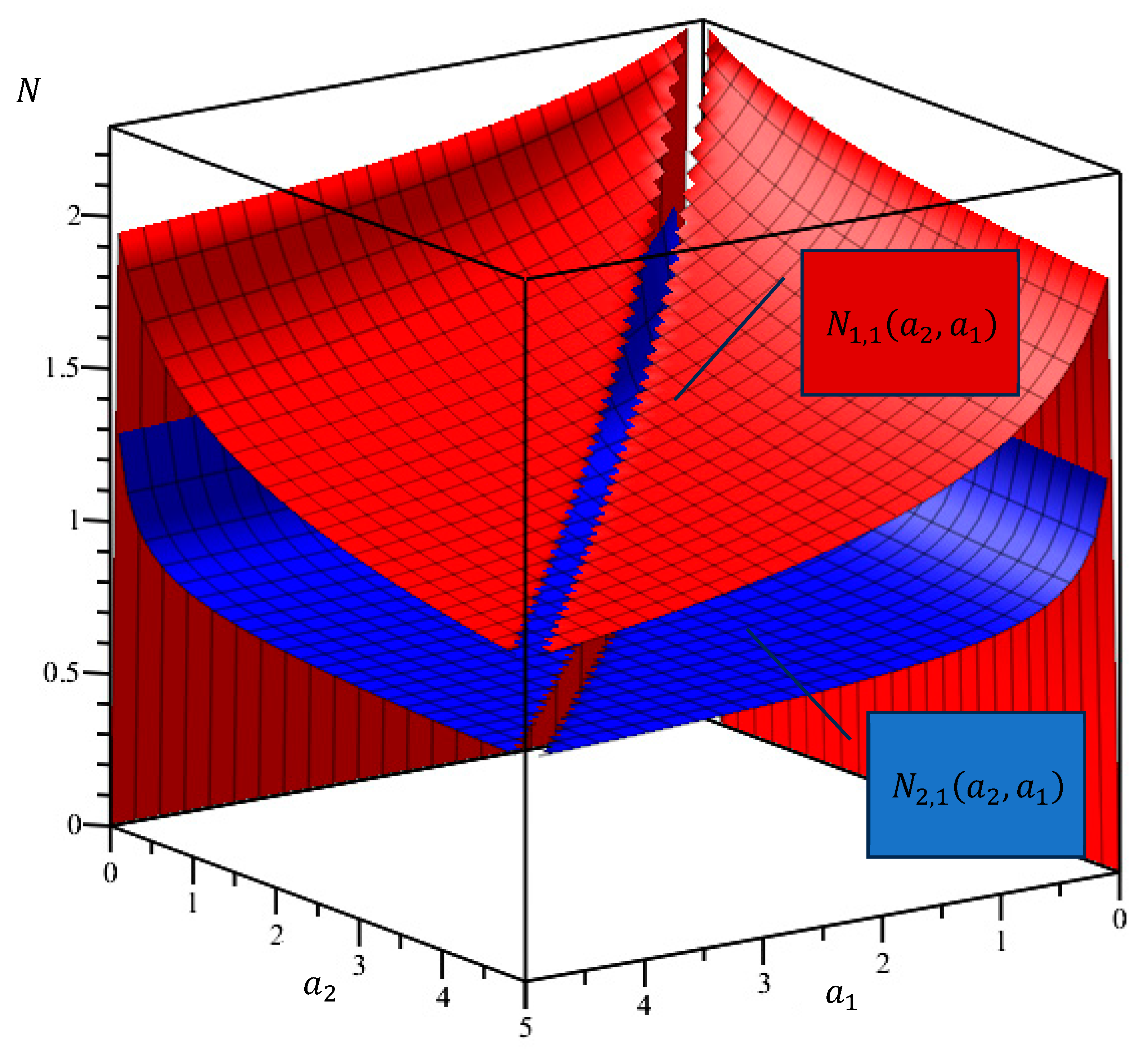
Figure 2.
The logarithm of the ratio of number of cycles required for a crack to grow from length a2 to length a1 for both kinds of equations (3) and (16). Source: Authors own work
Figure 2.
The logarithm of the ratio of number of cycles required for a crack to grow from length a2 to length a1 for both kinds of equations (3) and (16). Source: Authors own work

Figure 3.
The logarithmic plots of the number of cycles required for a crack to grow from the constant small length to length a_1 for both kinds of equations (3) and (16) for λ=1, c=1. Source: Authors own work.
Figure 3.
The logarithmic plots of the number of cycles required for a crack to grow from the constant small length to length a_1 for both kinds of equations (3) and (16) for λ=1, c=1. Source: Authors own work.

Figure 4.
The logarithmic plots of the number of cycles required for a crack to grow from the constant small length to length a_1 for both kinds of equations (3) and (16) for =1/2. Source: Authors own work
Figure 4.
The logarithmic plots of the number of cycles required for a crack to grow from the constant small length to length a_1 for both kinds of equations (3) and (16) for =1/2. Source: Authors own work
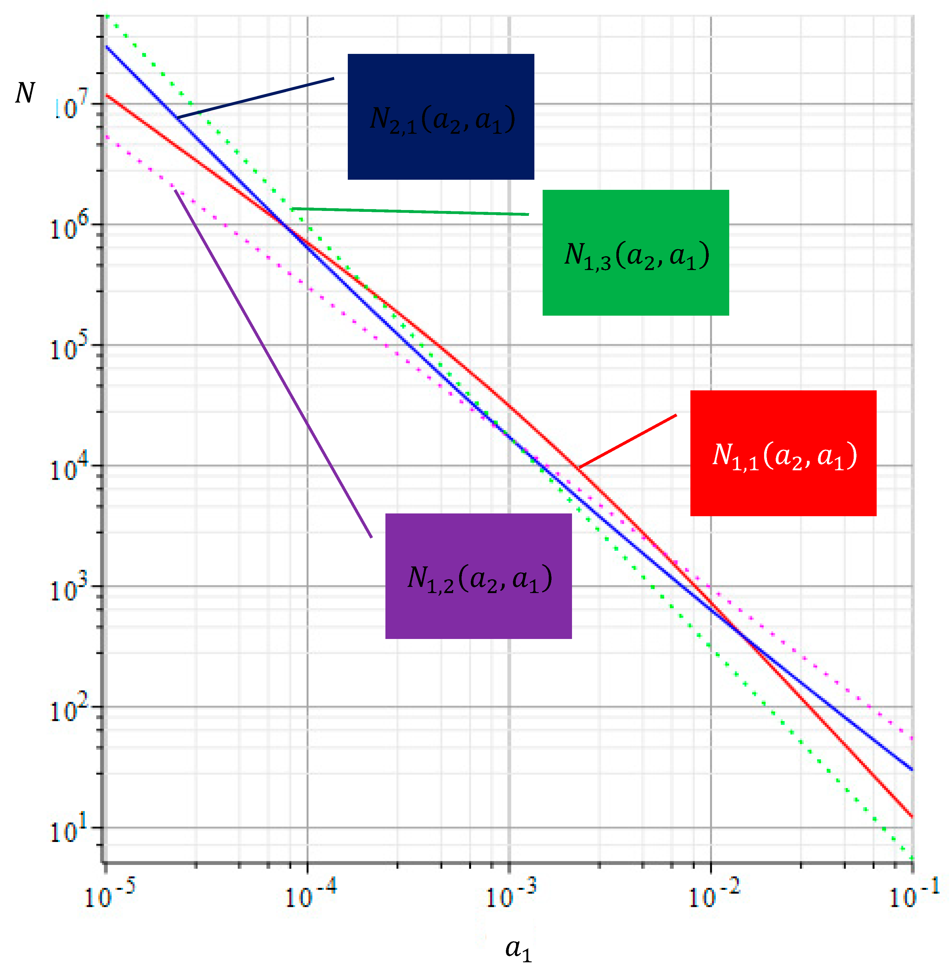
Figure 5.
The logarithmic plots of the number of cycles required for a crack to grow from the constant small length to length a_1 for both kinds of equations (3) and (16) for 3/2. Source: Authors own work
Figure 5.
The logarithmic plots of the number of cycles required for a crack to grow from the constant small length to length a_1 for both kinds of equations (3) and (16) for 3/2. Source: Authors own work
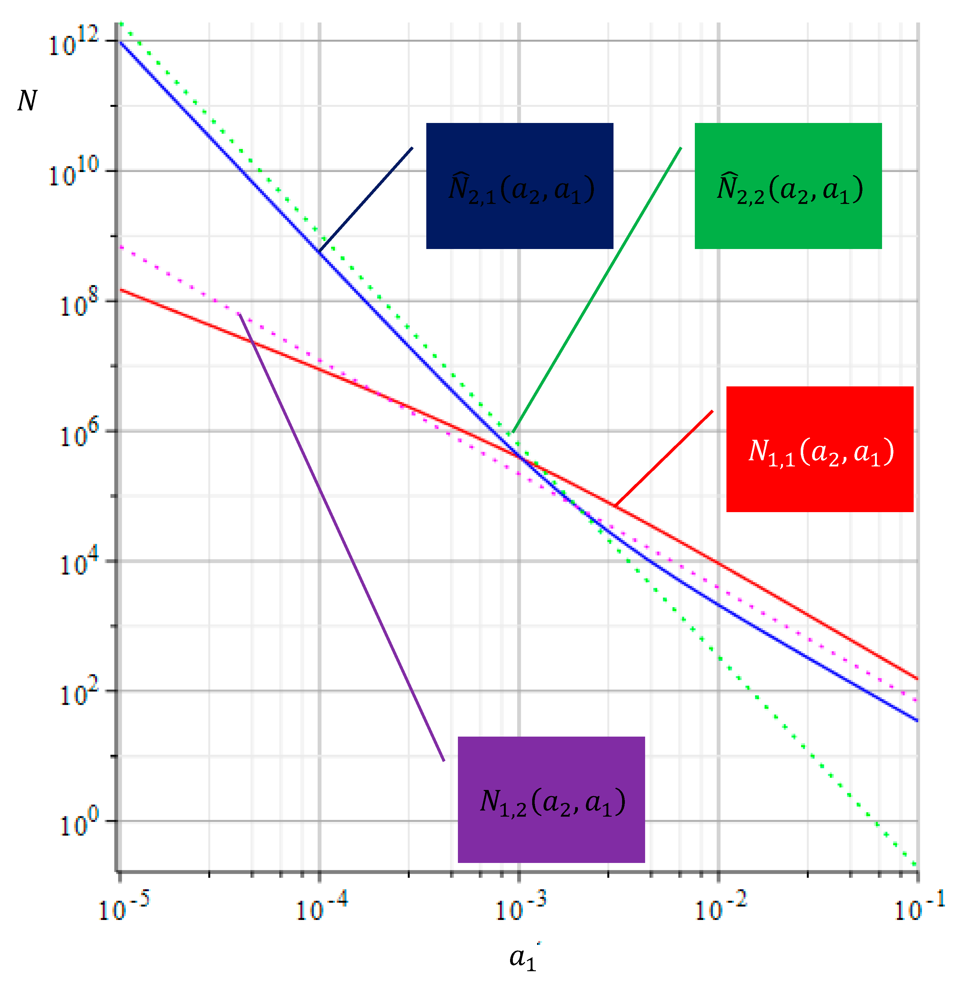
Figure 6.
The plot of the relations between the crack growth rate dn/da≡D0 [n(a)]=U_e (K)/c and the range of stress intensity factor K for aluminum alloys X-7075 and 7075 (Albrecht, 1976) Source: Authors own work.
Figure 6.
The plot of the relations between the crack growth rate dn/da≡D0 [n(a)]=U_e (K)/c and the range of stress intensity factor K for aluminum alloys X-7075 and 7075 (Albrecht, 1976) Source: Authors own work.
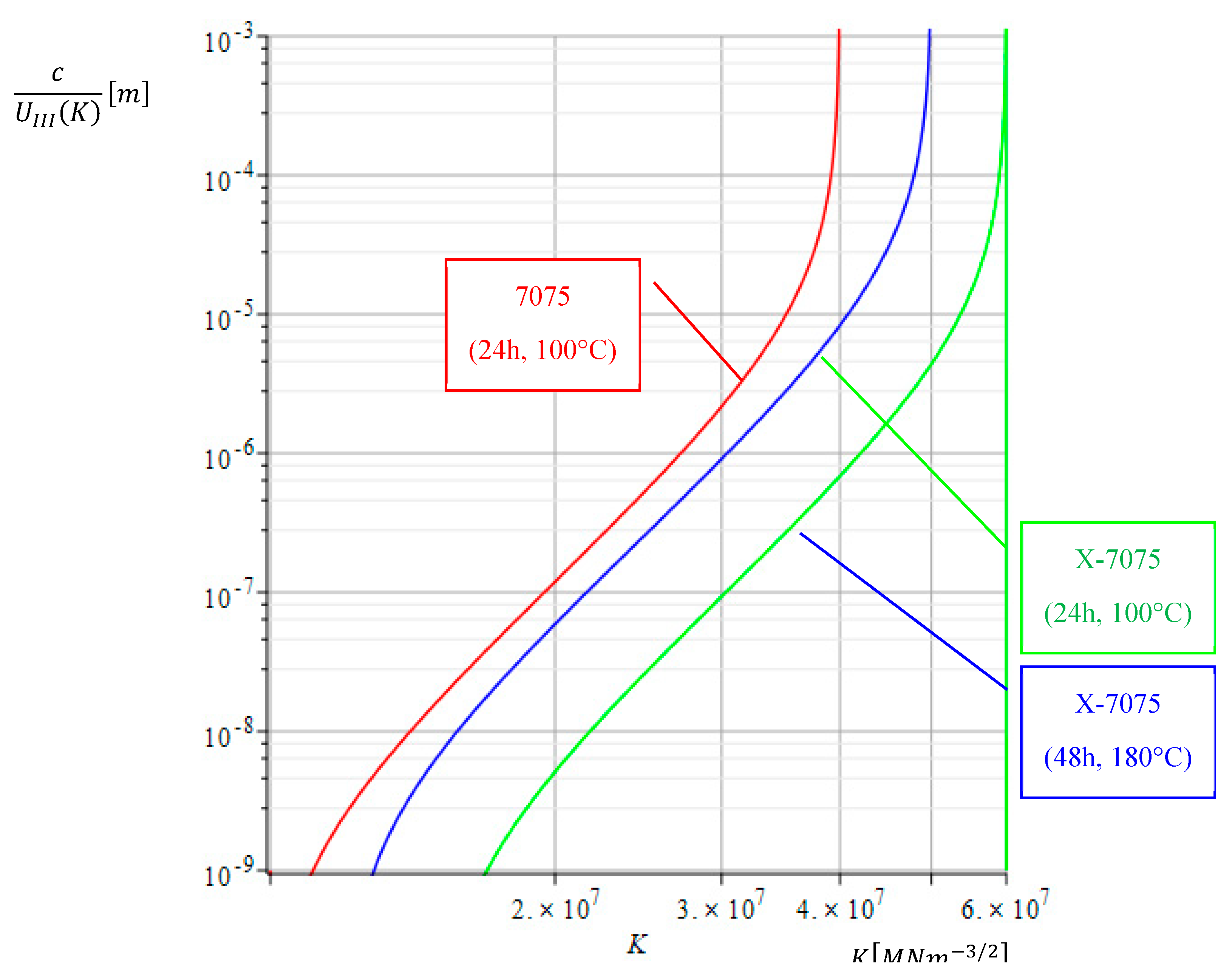
Figure 7.
The dependencies between the cycles to failure N for the given initial crack lengths upon the stress amplitude λ (s-N-curve) Source: Authors own work.
Figure 7.
The dependencies between the cycles to failure N for the given initial crack lengths upon the stress amplitude λ (s-N-curve) Source: Authors own work.
Disclaimer/Publisher’s Note: The statements, opinions and data contained in all publications are solely those of the individual author(s) and contributor(s) and not of MDPI and/or the editor(s). MDPI and/or the editor(s) disclaim responsibility for any injury to people or property resulting from any ideas, methods, instructions or products referred to in the content. |
© 2025 by the authors. Licensee MDPI, Basel, Switzerland. This article is an open access article distributed under the terms and conditions of the Creative Commons Attribution (CC BY) license (http://creativecommons.org/licenses/by/4.0/).
Copyright: This open access article is published under a Creative Commons CC BY 4.0 license, which permit the free download, distribution, and reuse, provided that the author and preprint are cited in any reuse.


