
Submitted:
20 April 2025
Posted:
21 April 2025
You are already at the latest version
Abstract
The capacity and generation of wind, solar, storage, nuclear, and gas are estimated for large, idealized copper plate electric grids. Wind/solar penetrations of 30% to 80% are considered together with different storage systems such as vanadium and lithium-ion batteries, pumped hydroelectric, compressed air, and hydrogen. In addition to a baseline dispatchable fleet without wind/solar, two bounding cases with wind/solar are analyzed: one without storage and one where the whole wind/solar fleet is connected to the storage system, hence providing a buffer between the wind/solar fleet and the grid. The reality will likely be somewhere between these bounding cases. The viability of a power grid with a large wind/solar penetration and no storage is not guaranteed but was nonetheless considered to provide a lower bound capital cost estimate. Overall, the options that rely strongly on wind/solar/storage may be more capital intensive than those that rely strongly on nuclear depending on the amount of storage necessary to ensure grid stability. This is especially true in the long run because wind/solar/storage assets have shorter operational lives than nuclear plants and, consequently, need to be replaced more frequently. More analyses (including grid stability and public acceptance) are necessary to determine which option is most likely to provide the path of least resistance to powering a clean, affordable and reliable grid in a timely manner. Depending on the priorities, the path of least resistance may not necessarily be the one that is less capital intensive.
Keywords:
Wind
; Solar
; Storage
; Nuclear
; Grid
; Adequacy
; Cost
1. Introduction
This paper presents some resource adequacy and capital cost considerations regarding the deployment of a large fleet of wind, solar photovoltaic (WS), and grid-scale storage on an idealized power grid. Though simplified, this approach enables useful comparisons highlighting relative differences between options. WS penetrations of 30 to 80% are considered. The WS fleets considered are scaled-up versions of the actual U.S. WS fleet, whose characteristics can be found on the U.S. Energy Information Administration (EIA) grid monitor portal. This idealized grid serves a large country, or a group of smaller countries or regions which need between 540 and 720 GW, with an average power of 600 GW (Figure 1).
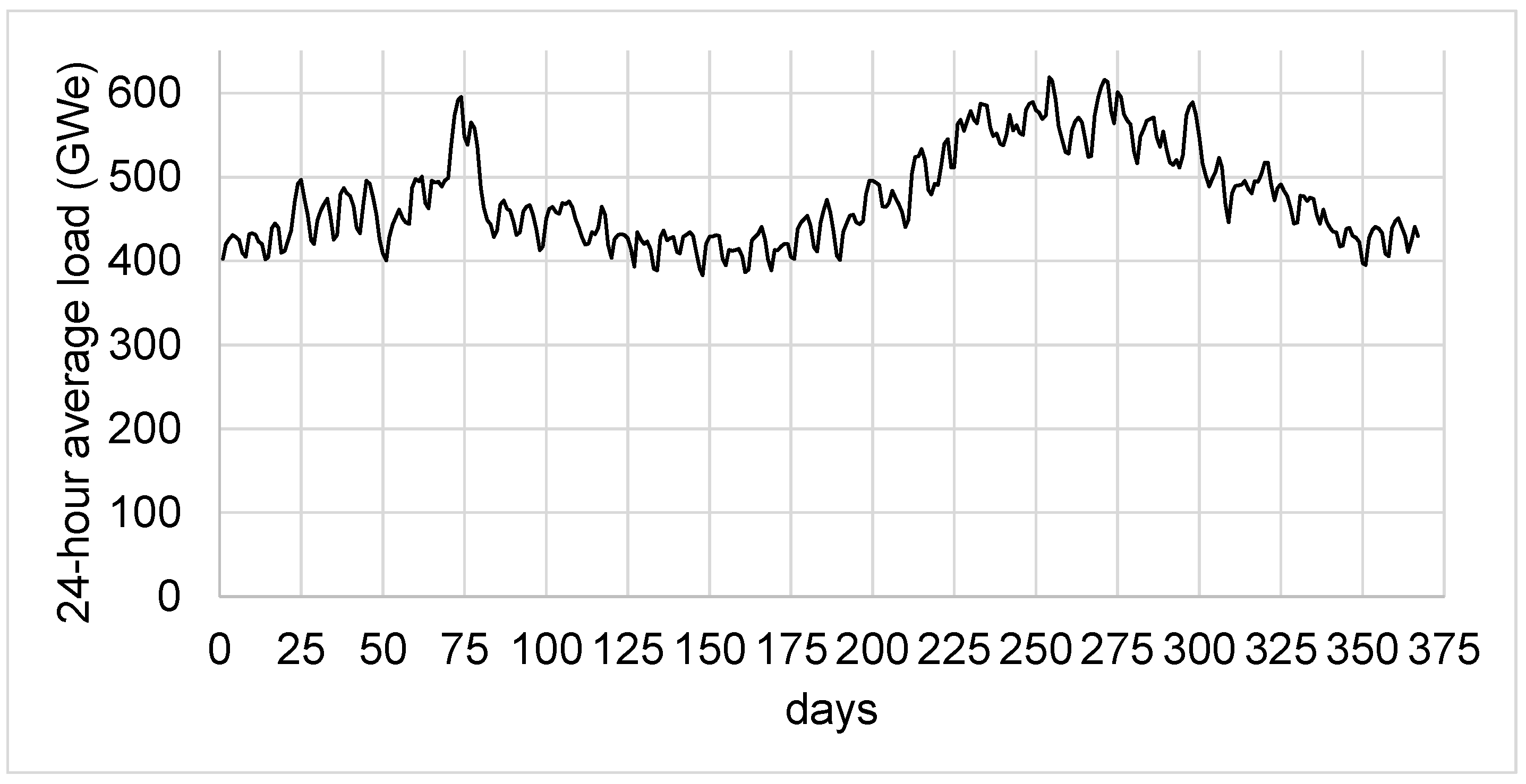
The corresponding annual electricity production is 5256 TWh or, equivalently, 600 GWy. This is about 25% more than what the U.S. currently needs (Figure 2). In its Annual Energy Outlook 2025 Reference Scenario, the EIA expects the U.S. demand to grow to that level by about 2045 [1].
Figure 1.
Illustrative grid load assumed for the sake of discussion. Average load = 600 GW.
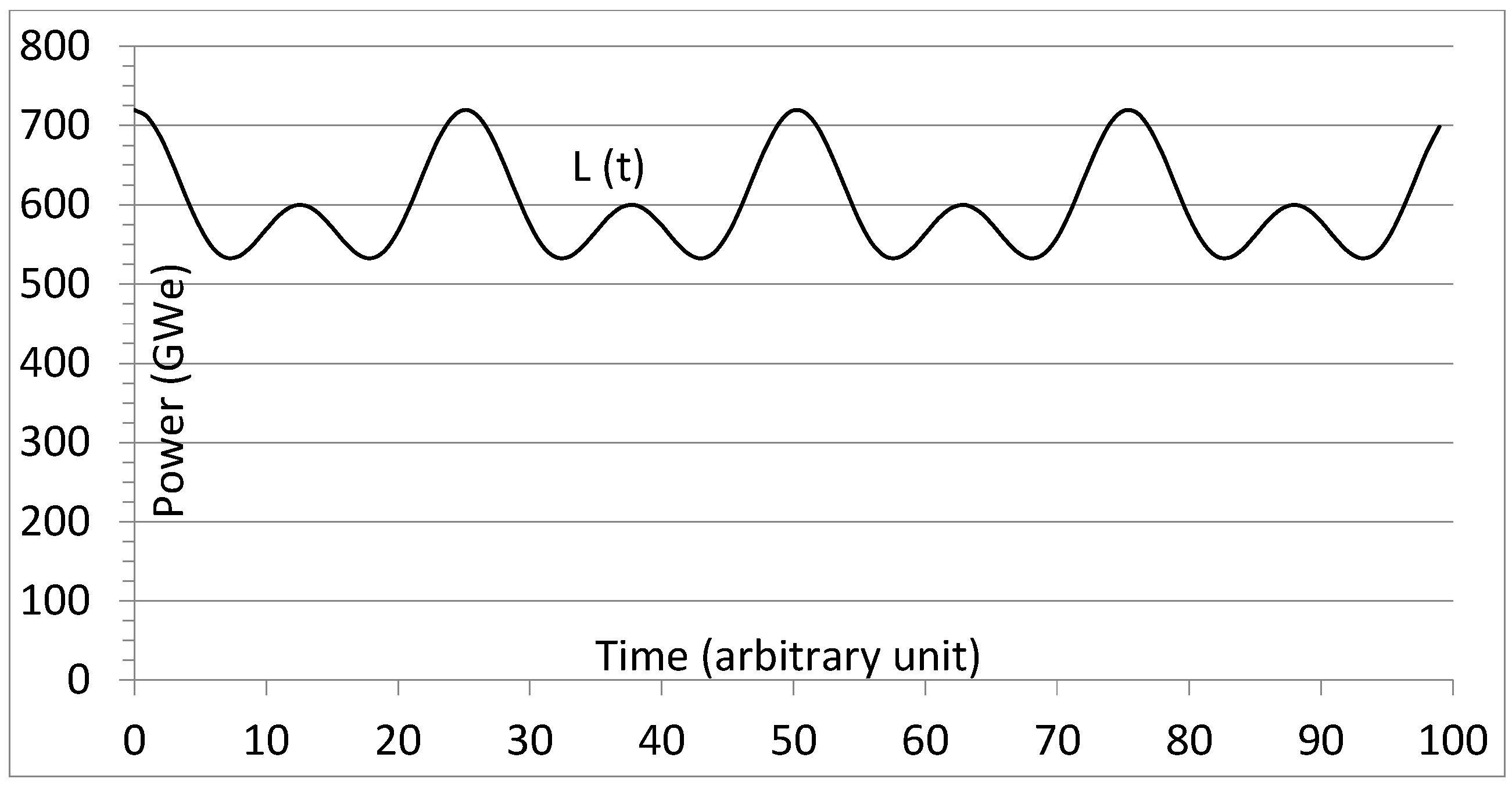
Figure 2.
Actual US grid load data between 11/5/2023 and 11/5/2024. Average load = 475 GW.
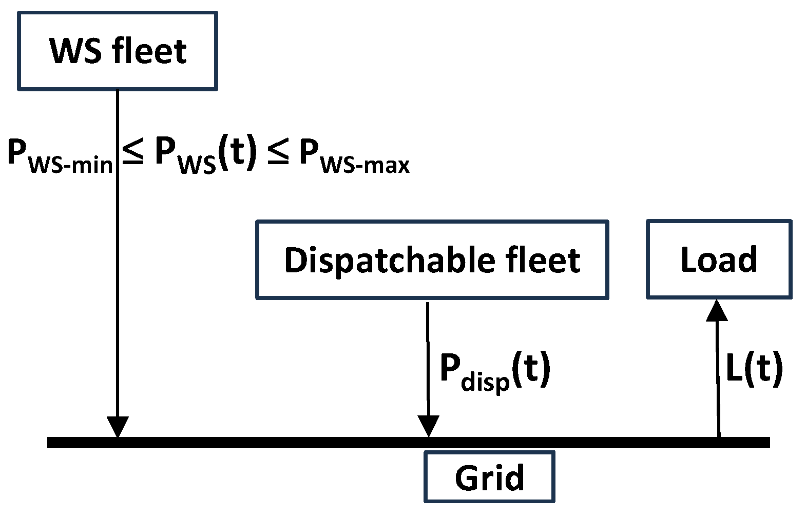
The load, L, satisfies the following expressions:
To simplify the discussion, the idealized grid is fully interconnected and without transmission losses (i.e., copper plate grid) so that electricity can flow unhampered from high quality WS location to high-quality storage locations or directly to distant load centers. This is an optimistic assumption and is central to enabling WS to contribute efficiently to the load. It is less important for the deployment of baseload power such as nuclear power plants. An actual grid will require more WS and storage capacity than this idealized grid to reach the same penetration.
Finally, the power system is assumed to be large enough to be considered an isolated system, i.e. supply and demand (i.e., load) must match without having recourse to an outside power grid either to export excess power or import power. The notion of an isolated system is important because it makes it necessary for the system designers and policy makers to fully internalize the consequences of the variability of the WS fleet. The U.S. grid almost satisfies this criterion because the exchanges of electricity with neighboring states (Canada and Mexico) are small compared to the electricity generated from within.
2. Baseline: No Wind, No Solar PV, Only Dispatchable Power
In the reference case, the load is met only with dispatchable thermal power generation such as fossil (coal and natural gas), nuclear, hydroelectric or geothermal (Figure 3).
Figure 3.
Illustration of the grid without WS.
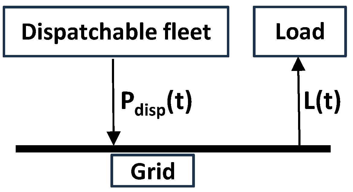
The power generated by the dispatchable fleet must satisfy the following in real time:
is the dispatchable nameplate capacity (the maximum power it can deliver to the grid), is the availability function at time t (fraction of the fleet that is available to generate power, i.e., not shut down for maintenance), and is the load following function at time t (the fraction of the available fleet called on by the grid to deliver power). It is assumed that, on average over any given year, the dispatchable power plants are down 15% of the time for maintenance and can generate their nominal power the rest of the time if needed. In other words, the yearly average of is 0.85. The load following function is equal to 1 for baseload plants and varies between 0 and 1 for load following plants. The instantaneous capacity factor of the dispatchable fleet, , is equal to . With these assumptions, the yearly average capacity factor is 0.85 for baseload plants and less than 0.85 for load following plants. Actual yearly average capacity factors for different technologies can be found, for example, in Reference [2].
At = , when the load is maximum, is, by definition, equal to 1 for all the power plants, i.e., . If, as a first approximation, is substituted by the average value, i.e., 0.85, then .
Under these assumptions, 847 GW of dispatchable plants () are necessary to ensure the 720 GW peak load is covered with sufficient confidence. In practice, more detailed analyses are of course necessary to determine the size of the fleet needed to meet the appropriate grid reliability criteria. As already mentioned, the load is assumed to vary between 540 and 720 GW with an average of 600 GW. One part of the fleet operates as baseload while the other follows the load. For instance, 588 GW of baseload plants could cover the load up to 500 GW (500/0.85) and 259 GW of load following plants between 500 and 720 GW (220/0.85) (see Figure 4).
The CO2 emission of a dispatchable fleet depends on the proportions of fossil fuel generation (coal, gas) and CO2-free generation (e.g., hydro, nuclear, geothermal). Overnight capital costs estimated by the U.S. EIA, natural resource consumption of coal, gas and nuclear power plants are shown in Table 1. The design lifetime of combined-cycle gas power plants is nominally 25-30 years, but many operators intend to extend it to 40-45 years [3]. A lifetime of 35 years was considered for gas power plants. Nuclear power plants are expected to operate for at least 60 years and modern coal power plants for 50-60 years.
To account for the operational lives of each technology, capital costs necessary for 60 years of operation are also presented in Table 1, assuming a zero discount rate and no credit for potential recycling of systems and components of assets with operational lives shorter than 60 years. The rationale for using a zero discount rate is presented in the next section. Sixty years of operation was chosen as a useful benchmark because it corresponds to the longest asset operational life, i.e. that of nuclear plants. With this approach, the capital cost expenditure over 60 years is simply the initial capital cost multiplied by [60 years ÷ asset operational life]. For example, if an asset has an operational life of 30 years and an overnight capital cost of $1.5B/GW, the estimated capital cost expenditure over 60 years is $3.0B/GW/60y. This simplified approach has the benefit of providing a lower and upper estimate of the capital cost expenditure with assets having different operational lives.
Figure 4.
Illustration of the baseload and load following distribution.
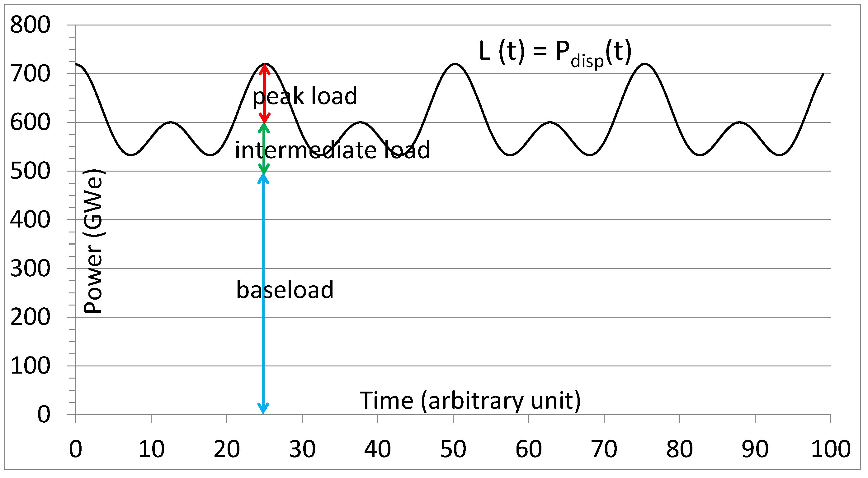

Table 1.
Thermal power plants characteristics.
| Natural Resource |
Techno. | Useful Life (Years) |
Net Efficiency (%) [4] |
Nat. Resource Consumption (MTA/GWy) |
Overnight Cap. Cost [4] ($B/GW) | Capital Cost Over 60 yrs ($B/GW/60y) |
| Coal | USCB | 50 | 39.5 | 3.4 million | 4.1 | 4.9 |
| Gas | CTC / CCD | 35 | 37.3/54.4 | 1.8/1.2 million | 0.84/0.92E | 1.4/1.6E |
| Uranium | PWRF | 60 | 32.2 | 150-210G | 7.9 | 7.9 |
(A) Metric Ton = 1000 kg. (B) Ultra-Supercritical. (C) Combustion Turbine, Single Cycle. (D) Combined Cycle. (E) The average values are considered for the cost estimations in the next sections, i.e., $0.88B/GW and $1.5B/GW/60y. (F) Large Pressurized Water Reactor (PWR) such as, for example, the AP1000 [5]. (G) U enrichment = 4.95%, average fuel burnup at discharge = 55-60 MWd/kg [6], U tail enrichment = 0.10%-0.25%.
If all 588 GW of baseload capacity is provided by nuclear power plants, and all 259 GW of load follow from gas power plants, the grid is 83% CO2-free and the capital cost is $4.9T, i.e., $5.0T/60y (Table 2). This dispatchable fleet provides a useful benchmark to compare the other fleets with. Most importantly, this dispatchable low-CO2 fleet provides a reference point to determine whether less capital-intensive fleets are possible by introducing WS and storage.
Table 2.
Installed capacity and annual electricity generation of the reference dispatchable-only fleet.
Table 2.
Installed capacity and annual electricity generation of the reference dispatchable-only fleet.
| Capacity (GW) | Gene (GWy) | |
| Baseload (Nuclear) | 588 | 500 |
| Load Follow (Gas) | 259 | 100 |
| Total Fleet | 847 | 600 |
| % CO2-free | 83 | |
| Initial Capital Cost ($T) | 4.9 | |
| 60-year Capital Cost ($T/60y) | 5.0 | |
3. The Zero Discount Rate Rationale
The analysis in this example assumes a discount rate of zero because the purpose of the example is to focus on resource utilization and not a financial consequence to a specific entity. That is, a monetary estimate of cost represents a metric to measure the quantity of resources used over the lifetime of the project. Assuming a non-zero discount rate implies subjective value in the concept of the time value of money, which is not the intent of the example. And if one chooses to apply the time value of money, then one must decide whose value is to be represented.
The choice of which discount rate should be applied in an analysis is a topic of considerable debate in the literature [7]. Economic reasoning suggests that identifying the purpose of the discount rate is a necessary but not sufficient condition [8]. For example, discounting public sector investments requires different assumptions than those underlying the discount rate choice for private sector investments [9]. Whereas the discount rate adjusts cash flows for the effects of financial risk and opportunity cost, neither of these can be identified without defining whose risk and cost.
The underpinnings of discounting cash flows date to Ramsey’s seminal work where the underlying components of the discount rate are derived in relation to the decision on savings versus consumption [10]. That is, decision maker’s rate of time preference, consumption, and projected economic growth play a role, as do systematic and non-systematic risks in the investment.
Because the aim of the example is to illustrate resource utilization across energy generation alternatives, and not the complexities of identifying which discount rate is best, zero discounting applies.
4. Deploying the WS Fleet Without Storage
The power generated by the WS and dispatchable fleets (Figure 5) must satisfy the following in real time:
is the WS nameplate capacity (the maximum power it can deliver to the grid), is the WS fleet availability function (fraction of the WS fleet that is available to generate power, i.e., not shut down for maintenance), and is the fraction of the available WS fleet delivering power to the grid. The instantaneous capacity factor of the WS fleet, , is equal to . The assumed yearly average capacity factor of the WS fleet is 30%, i.e., like that of the actual US WS fleet (in 2023, the yearly average capacity factors of the ~150 GW wind fleet and of the ~125 GW solar PV fleet were 33% and 23%, respectively) [11].
with an assumed yearly average equal to
In other words: , , and
Figure 5.
Illustration of the grid with WS and without storage.
Grid stability aspects are not explicitly treated here, but it is important to note that the viability of a power grid with a large WS penetration and no storage is not guaranteed. The reason is that ensuring the power delivered by the dispatchable fleet, , matches the residual load, , in real time is more challenging than just ensuring it matches the actual load, , as for the reference case without WS. The no-storage cases were nonetheless considered to provide lower bound capital cost estimates.
The assumed yearly average capacity of our WS fleet is 30%. This could be, for example, a WS fleet with equal installed capacity of wind and solar where = 0.35 and = 0.25. The estimated operational life of both wind turbines and PV systems is about 30 years [12,13]. Capital cost is about $1.5B/GW for both PV and onshore wind turbines [4]. Consequently, using the approach described in section 2, the capital expenditure over a 60-year period is $3.0B/GW/60y.
The extent of fluctuations, the [-] range, depends on factors such as the location of the WS fleet and its composition (i.e., the respective fractions of wind and solar). This is a crucial attribute of the WS fleet because it strongly impacts the composition and size of the dispatchable fleet needed to ensure an appropriate power supply to the grid. The WS penetrations considered here (30-80%) are larger than the current one (15%). Consequently, the dispatchable fleet needs to accommodate higher ramp rates than is currently the case to compensate for the variability of the WS fleet. This has consequences for the power plants that are not addressed here. It is assumed that the dispatchable fleet will adjust accordingly.
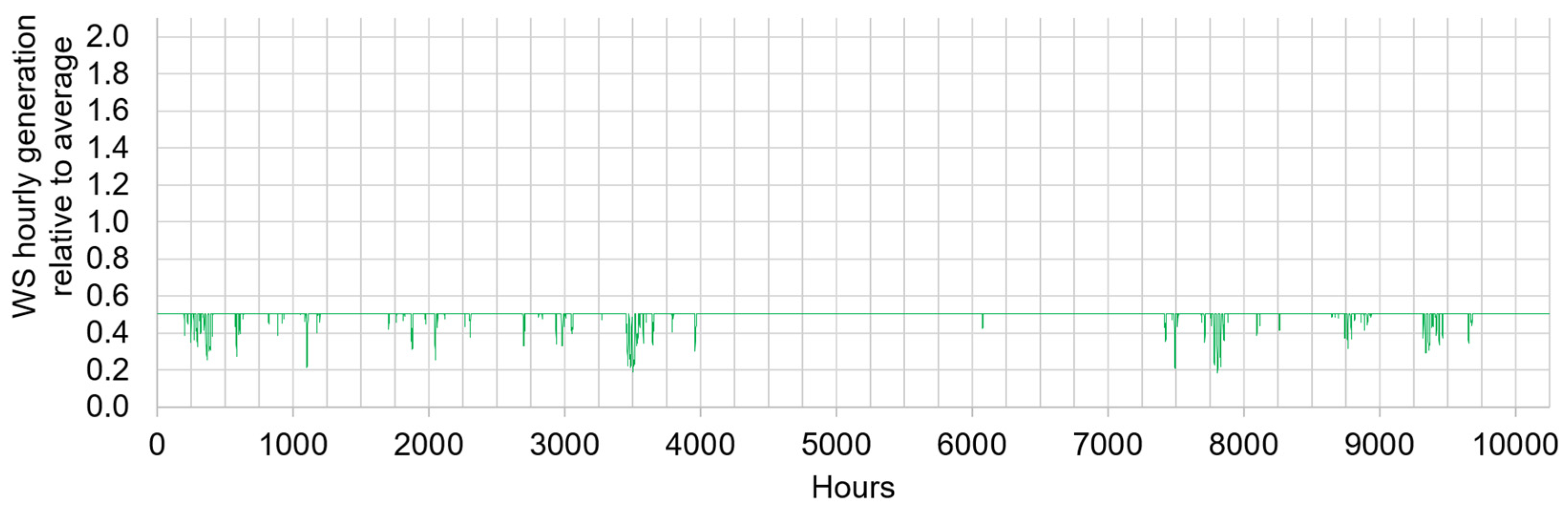
An indication of the potential [-] range can be found in the U.S. electric grid data maintained by the EIA [14]. The data corresponding to the actual U.S. WS fleet between 09/01/2023 and 10/31/2024 is shown in Figure 6.
Figure 6.
Hourly generation of the actual U.S. WS fleet relative to the average (72 GWh) between 09/01/2023 and 10/31/2024.
Figure 6.
Hourly generation of the actual U.S. WS fleet relative to the average (72 GWh) between 09/01/2023 and 10/31/2024.
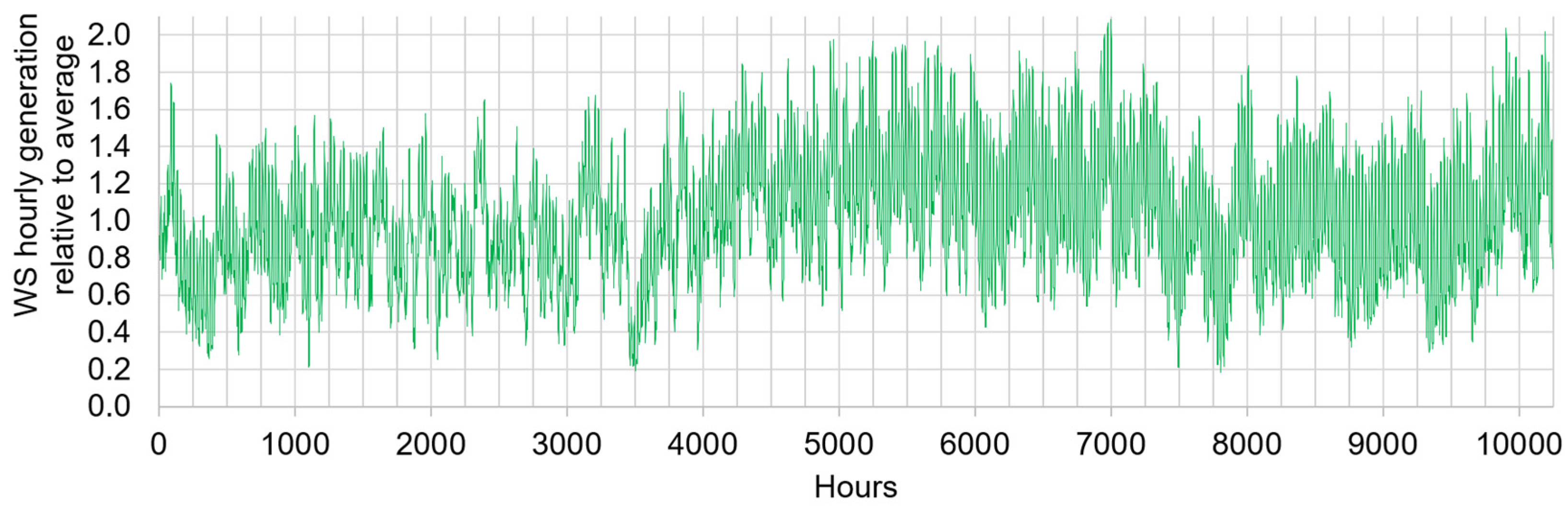
During that time, it produced on average 72 GW (50 GW from W; 22 GW from S) with maximum and minimum hourly averages of 150 GW (6/18/2024 @ 2 p.m. EST) and 13 GW (07/22/2024 @ 7 a.m. EST), respectively. In other words, the maximum and minimum hourly average were 2.1× and 0.18× the average, respectively. Applying these factors to our WS fleet, neglecting the intra-hour fluctuations as a first approximation, the instantaneous capacity factor varies between = 0.054 (0.18 × ) and = 0.63 (2.1 × ).
As mentioned above, the [-] range has important consequences on the dispatchable fleet. The larger it is, the more baseload it displaces and the larger the ramp rate of the load following plants is. With this respect, curtailment could be useful to minimize the [-] range. A curtailed WS fleet, WS*, satisfies the following:
The α/β couples obtained from the reference U.S. WS data are shown in Figure 7. For example, the couple 0.95/1.3 satisfies the equations above. In other words, if the reference U.S. WS fleet was curtailed when its power exceeded 1.3, it would still deliver to the grid 95% of the electricity generated by the reference, non-curtailed fleet. The [-] range is reduced by 42% ([1.3-0.18]÷[2.1-0.18]) compared to that of the non-curtailed case for a 5% loss of generation. The time series corresponding to three curtailed WS* fleets are shown in Figure 8, Figure 9 and Figure 10 as examples.
Figure 7.
Fraction of the non-curtailed WS generation as a function of the curtailment threshold.

It is noteworthy that the WS* power delivered to the grid becomes more predictable as the level of curtailment increases. For example, equals 22% of the time when the curtailment threshold is . When the curtailment threshold is , equals 75% of the time. And when the curtailment threshold is , equals 93% of the time. The benefits of increased predictability should be weighed against the energy lost due to curtailment. Ideally, the energy generated by the WS fleet when it exceeds the grid curtailment threshold would be used for off-grid applications better suited to cope with large power fluctuations, assuming such applications exist.
Figure 8.
Hourly generation of the U.S. WS fleet relative to the average assuming curtailment when which corresponds to 5% lost generation.
Figure 8.
Hourly generation of the U.S. WS fleet relative to the average assuming curtailment when which corresponds to 5% lost generation.
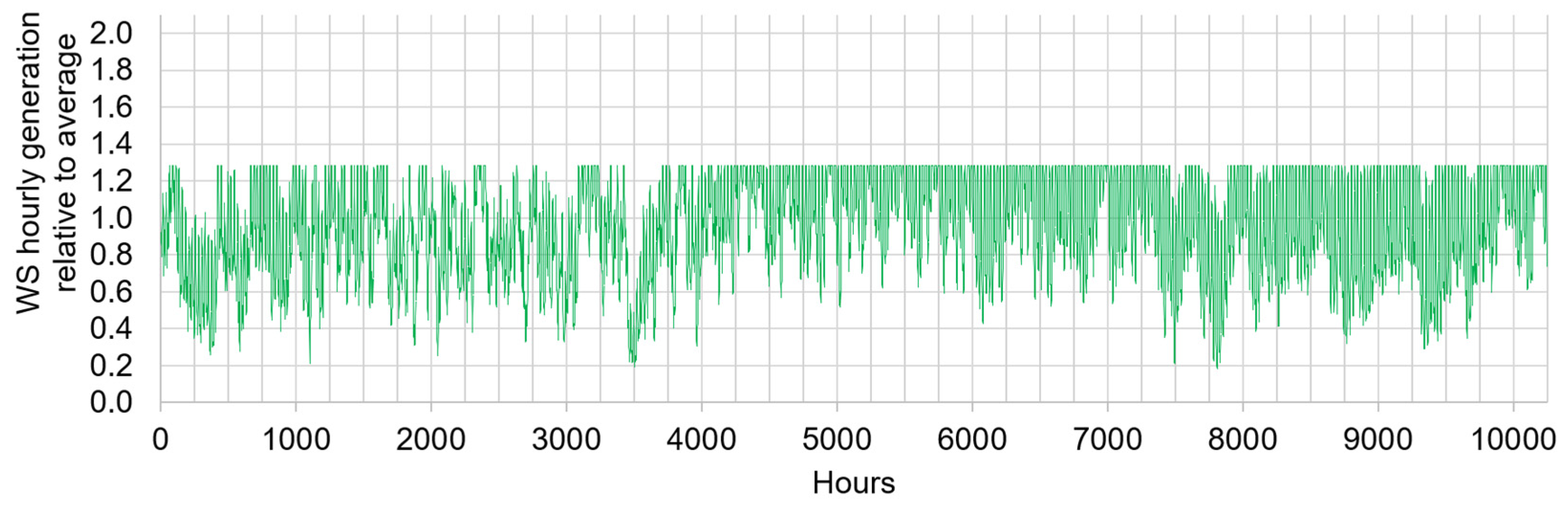
Figure 9.
Hourly generation of the U.S. WS fleet relative to the average assuming curtailment when which corresponds to 30% lost generation.
Figure 9.
Hourly generation of the U.S. WS fleet relative to the average assuming curtailment when which corresponds to 30% lost generation.
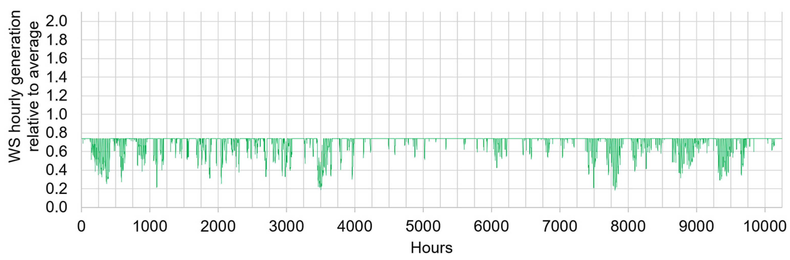
Figure 10.
Hourly generation of the U.S. WS fleet relative to the average assuming curtailment when which corresponds to 50% lost generation.
Figure 10.
Hourly generation of the U.S. WS fleet relative to the average assuming curtailment when which corresponds to 50% lost generation.
5. Deploying the WS Fleet with Storage
The energy storage systems of interest here should be scalable to 100s of GW. The whole WS fleet is assumed to be connected to it, as illustrated in Figure 11.
Figure 11.
Illustration of the grid with WS and with storage.
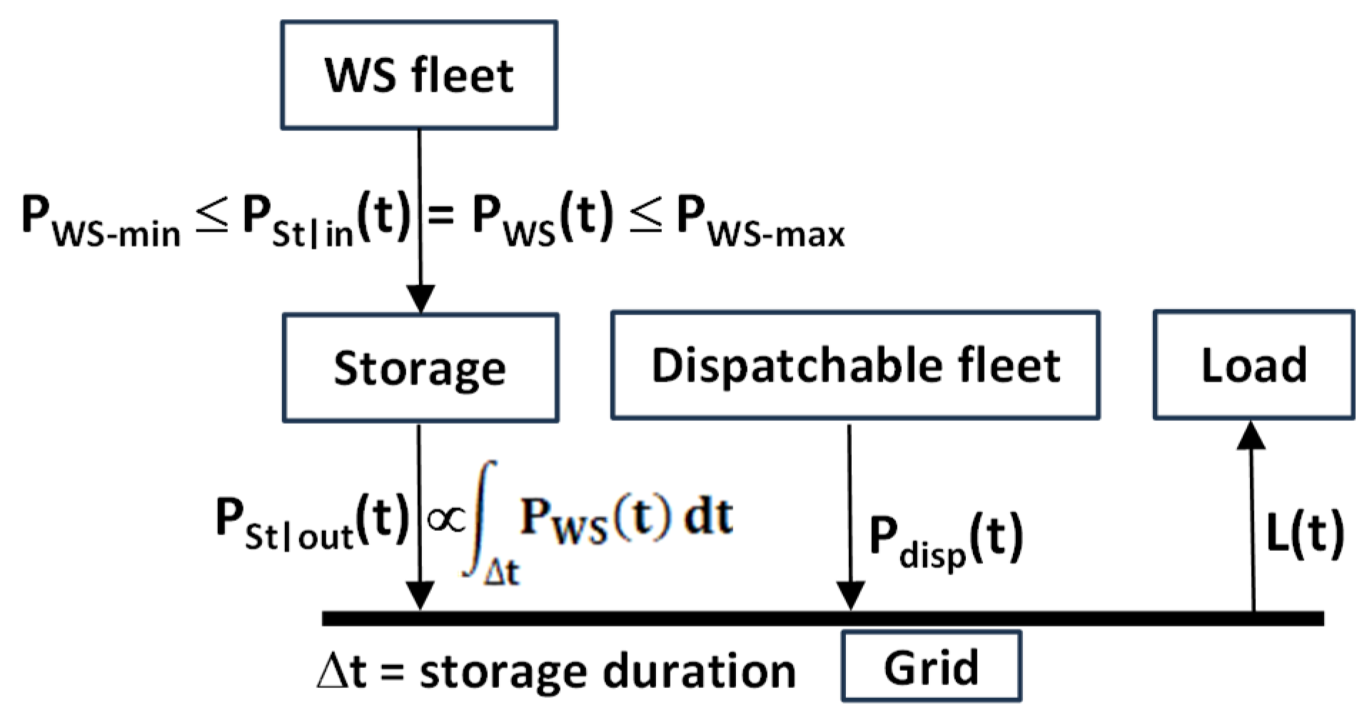
The energy storage system acts as a buffer, or integrator, between the WS fleet and the grid. It also contributes to grid stability. Just like curtailment, energy storage mitigates the rate and amplitude of the fluctuations of the power delivered to the grid and, consequently, makes it more predictable. Since curtailment and energy storage both increase predictability, it seems reasonable to expect that a curtailed WS fleet may require less energy storage than a non-curtailed WS fleet to reach the same level of predictability.
The underlying assumption is that, as WS penetration increases, future WS operators will be required to contribute some degree of firmness to the grid by using storage. The degree of firmness increases with the storage duration as well as with the curtailment level. The round-trip efficiency (RTE) of a storage system is defined as the kWh-out/kWh-in ratio. The storage system and the dispatchable fleet satisfy the following requirements:
with and is the power used to charge the storage system; It is equal to . is the power delivered to the grid by the storage system. Δt is the storage duration (4, 24, and 100 hours were considered). fluctuates less and less as the storage duration increases. In other words, the degree of firmness of the storage system increases with its duration and, consequently, its ability to replace dispatchable thermal power plants also increases. is more predictable than and, consequently, it is less challenging to ensure the power delivered by the dispatchable fleet, , matches in real time than to ensure it matches , as when there is no storage.
However, the inevitable inefficiencies of the storage systems require increasing the size of the WS fleet by a factor of 1/RTE compared to the WS fleet without storage to deliver the same energy to the grid. The power delivered to the grid by the storage system during an interval Δt is:
For example, if Δt = 24 hours, the average power delivered by the storage system on any given day is equal to the average power generated by the WS fleet the day before multiplied by the storage system RTE (assuming there is no residual from previous days).
In the previous equation, is the storage nameplate capacity, i.e., the maximum power it can deliver to the grid; is the fraction of the storage nameplate capacity delivering power to the grid between t and t + Δt; is the availability function of the storage power conversion system between t and t + Δt (fraction of the storage fleet that it is available to generate power); is the fraction of the available storage nameplate capacity called on by the grid to deliver power between t and t + Δt. The availability function yearly average is assumed to be 0.85. The storage nameplate capacity, , depends on the system characteristics. Four types of storage are possible (A, B, C, D).
∙ Type-A can charge with and charge/discharge concurrently. Storage systems such as pumped hydro (PHS), compressed air energy storage (CAES), or power-to-hydrogen-to-power (P2H2P) (see Section 6) have separate charge and discharge processes and subsystems and, consequently, either are type-A or could in principle be modified to be type-A. In the time interval Δt, when the storage system delivers its maximum power, , by definition, is equal to 1. If, as a first approximation, is substituted by its average value of 0.85, then, the nameplate capacity can be expressed as
Storage system A must be able to store up to .
∙ Type-B can charge with but cannot charge/discharge concurrently. Consequently, the type-A storage system must be doubled, and the nameplate capacity is:
Storage system B must be able to store up to ∙ Type-C cannot charge with but can charge/discharge concurrently. In this case the nameplate capacity must be equal to , i.e., divided by the availability of the storage system.
Storage system C must be able to store up to ∙ Type-D cannot charge with and cannot charge/discharge concurrently. Consequently, the type-C storage system must be doubled. Batteries typically belong to this category. The nameplate capacity is
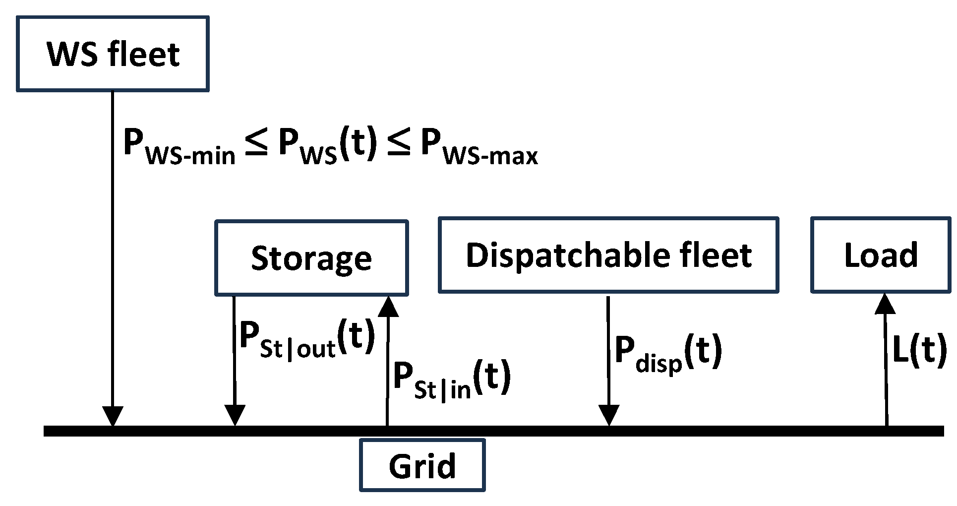
Storage system D must be able to store up to Finally, it is noteworthy that the storage configuration of interest here (Figure 11) is conceptually and operationally different from how most storage systems currently operate (Figure 12). In this case the storage system does not act as a buffer between the WS fleet and the grid and is mainly used for energy arbitrage. With typically only one cycle/day it is also used less intensively than in Figure 11. This configuration satisfies:
Figure 12.
Illustration of how most grid storage systems currently operate.
6. Energy Storage Systems Considerations
This section may be divided by subheadings. It should provide a concise and precise description of the experimental results, their interpretation, as well as the experimental conclusions that can be drawn.
6.1. Short-Duration Storage
For storage systems capable of storing energy for up to 4 hours, RTEs of 0.50-0.85 were considered. It is representative of a range of technologies such CAES (RTE ~ 0.5) [15], vanadium flow batteries energy storage (BES) (RTE = 0.65) [16], PHS (RTE=0.80) [17], and lithium-ion BES using a lithium iron phosphate (LFP) cathode (RTE = 0.85) [18].
The U.S. has 43 PHS plants with an estimated energy storage capacity of 553 GWh; the largest (Bath County) has a maximum generation capacity of 3 GW and a total storage capacity of 24 GWh. A resource assessment performed by the National Renewable Energy Laboratory (NREL) concluded that there are sufficient sites in the contiguous U.S. to generate up to 27 TWh [19] (2700 GW for 10 hours) with PHS, equivalent to 49× the current capacity.
As of 09/2024, the U.S. also had about 21 GW of utility-scale lithium-ion BES with an estimated energy storage capacity of 56 GWh [20]. Until it was recently destroyed by a fire, the largest LFP BES (Moss Landing, California) had a maximum generation capacity of 0.75 GW and total storage capacity of 3 GWh. Among the critical materials needed, LFP BES require about 0.08 kgLi/kWh [21], or 0.08 million metric tons of lithium per TWh. For comparison, recent estimates of worldwide lithium resources and annual production are about 105 and 0.18 million metric tons, respectively [22].
There is currently no vanadium BES in the U.S. to speak of. The largest vanadium flow BES (Dalian, China) has a maximum generation capacity of 0.1 GW and a total storage capacity of 0.4 GWh [23]. Vanadium flow BES have a typical power density of 20 kWh/m3 and vanadium concentration of 1-3 M (51-153 kgV/m3) [24]. Expressed differently, a vanadium flow BES system requires about 2.5-7.7 million metric tons of vanadium per TWh. For comparison, recent estimates of world vanadium resource and annual production are about 63 and 0.10 million metric tons, respectively [25]. Hence, vanadium BES are more resource limited than lithium BES.
Several small-scale CAES facilities have been built and operated around the world, including in the U.S. The largest one is currently located in Hubei, China. It has a maximum generation capacity of 0.3 GW, a total storage capacity of 1.5 GWh, and a claimed RTE of 0.64 [26]. The 0.11 GW McIntosh plant in Alabama has a total storage capacity of 2.6 GWh but is not entirely CO2-free as it also burns natural gas.
6.2. Long-Duration Storage
For storage systems capable of storing energy for 24 to 100 hours, a range of long-duration energy storage (LDES) technologies [27] was considered with RTEs of 0.30-0.80. This includes PHS, CAES, and P2H2P (RTE ~ 0.3) [28]. The 24-hour and 100-hour durations are long compared to the current mainstay 4-hour storage. Much longer durations (months) would however be necessary to get rid of most of the dispatchable power.
Assuming a power conversion system efficiency (gas turbine [29] or fuel cells) of 50%, 1 kg of hydrogen generates 16.7 kWh of electricity, whereas it takes about 45-55 kWh to create this kg through low-temperature water electrolysis. This corresponds to a P2H2P RTE of 0.30 to 0.37 (these values do not include losses during storage and transportation). The largest hydrogen electrolyzer (the P2H part of the P2H2P system) was manufactured by the Shuangliang Group (China) and was inaugurated in October 2024. It has the capacity to produce about 450 kg of hydrogen per hour (up to 3.94 million metric tons per year if operated 24/7) [30]. A resource assessment performed by NREL concluded that 9.8 million metric tons of pure hydrogen could be stored in existing U.S. underground gas storage facilities [31]. The largest hydrogen geological storage facility (in Utah) can store up to 11,000 metric tons [32].
6.3. Operational Life
PHS and CAES both have an estimated operating life of 60 years. For continuous baseload operation, the expected P2H2P electrolyzer stack lifetimes are 60,000 to 80,000 hours (7-9 years) of operation for proton exchanging membrane (PEM) and alkaline electrolyzers [33]. However, studies have shown that flexible operation, such as when powered by WS, may lead to shorter stack lifetime. DOE has set ultimate targets for fuel cell system lifetime under realistic operating conditions at 80,000 hours (9 years) for distributed power systems [34].
For 4-hour storage, lithium-ion LFP BES have an estimated life of 7300 cycles [35]. This corresponds to a 7.8-year life for the operating conditions of interest here, i.e., 3 cycles per day (24÷[2×4]) and an availability of 0.85 (7300÷[3×365×0.85]). Many references give longer BES lives because they consider only one cycle per day which implies the BES is mainly used for arbitrage purposes and not as a buffer between the WS fleet and the grid. The DOE Technology Strategy Assessments referenced previously yields a comparable life estimate; 2640 cycles for 10-hour storage lithium-ion LFP BES. This corresponds to a 7.1-year life for 1.2 cycles per day (24÷[2×10]) and an availability of 0.85 (2640 ÷ [1.2 × 365 × 0.85]). For 10-hour storage, vanadium BES are rated at 10,000 cycles (i.e., ~25,000 cycles for 4-hour storage). The corresponding vanadium BES operational life is 27 years.
6.4. Storage Overnight Capital Cost
Representative storage capital costs estimated by the U.S. Pacific Northwest National Laboratory for large 1 GW facilities in 2030 are presented in Table 3 for storage durations of 4-100 hours [36]. Table 4 shows the storage overnight capital cost that must be spent over a 60-year period ($B/GW/60y) using the zero discount rate approach described in Section 2. The short operational lives of P2H2P and Li-BES are particularly penalizing economically.
Table 3.
Storage overnight capital costs ($B/GW) for different storage technologies and durations.
| 4 hours | 10 hours | 24 hours | 100 hours | Operational Life (Years) |
RTE | |
| PHS | 1.7 | 2.2 | 2.9 | 6.9 | 60 | 0.80 |
| CAES | 1.1 | 1.1 | 1.2 | 1.6 | 60 | 0.50 |
| P2H2P | - | 1.0 | 1.1 | 1.5 | 9 | 0.30 |
| Li-BES | 1.1 | 2.5 | - | - | 8 | 0.85 |
| V-BES | 1.6 | 3.0 | 6.4 | - | 27 | 0.65 |
Table 4.
Storage overnight capital costs expenditure over 60 years ($B/GW/60y) for different storage technologies and durations.
Table 4.
Storage overnight capital costs expenditure over 60 years ($B/GW/60y) for different storage technologies and durations.
| 4 hours | 10 hours | 24 hours | 100 hours | |
| PHS | 1.7 | 2.2 | 2.9 | 6.9 |
| CAES | 1.1 | 1.1 | 1.2 | 1.6 |
| P2H2P | - | 6.7 | 7.3 | 10.0 |
| Li-BES | 8.3 | 18.8 | - | - |
| V-BES | 3.6 | 6.7 | 14.2 | - |
7. 30% Wind/Solar Penetration
A 30% WS penetration corresponds to approximately twice the current WS penetration of the U.S. grid. Power systems without storage and with storage are successively discussed.
7.1. No Energy Storage
The WS fleet delivers a yearly average of 180 GW to the grid, i.e., 30% of the average load of 600 GW. Since the yearly average WS capacity factor, , is also 30% the WS fleet nameplate capacity, , is 600 GW.
As mentioned in Section 4, based on existing data, it is assumed that the power delivered by our 600 GW WS fleet fluctuates between and . Since curtailment is not necessary. If it is deemed sufficiently unlikely that could be lower than this value, then it can be considered a firm capacity and, consequently, replace 38 GW of baseload power (32.4/0.85). Furthermore, 407 GW of baseload power must be replaced by 407 GW of fast-ramping load following plants ([378-32.4]/0.85) to compensate for potentially large and rapid fluctuations of the WS fleet. Out of the original 588 GW of baseload power (see Table 2-1), there remain 588 - 407 - 38 = 143 GW. If it cannot be ruled out with sufficient certainty that could happen concomitantly with peak load, then the same 259 GW of load following plants as before are needed to cover the load between 500 and 720 GW.
The resulting 1409 GW fleet is made up of 600 GW WS and 809 GW of dispatchable power (666 GW of load following plants and 143 GW nuclear baseload). It is 50% CO2-free (30% WS + 20% nuclear). Gas power plants would likely provide most of the necessary 666 GW of fast ramping load following capacity generating the other 50% of the electricity needed by the grid. The capital cost for this fleet is about $2.6T (0.90T WS, 0.59T gas power plants, 1.1T nuclear power plants) or $3.9T/60y.
The 809 GW dispatchable fleet could in principle meet the load without the WS fleet. The potential benefit of the WS fleet is that it may enable less fossil fuel consumption and, consequently, less CO2 emissions may result. This is, however, not necessarily the case. Indeed, even highly efficient power plants such as combined cycle gas turbines (CCGT) see their efficiency drop when they operate outside their range of optimal nominal operation. Consequently, they burn more fuel and emit more CO2 per kWh [37,38]. In other words, replacing highly efficient CCGT baseload power plants with a combination of WS and fast ramping gas power plants may not necessarily reduce CO2 emissions even if the fast ramping power plants generate overall fewer kWh than the baseload power plants that they replaced.
As discussed in Section 4, curtailment can be used to manage supply and demand. For example, if the power generated by a 632 GW WS fleet was curtailed when it exceeded 1.3× its average (189 GW), it would still generate on average 95% of the non-curtailed fleet, i.e., 180 GW. In this case the curtailed 632 GW WS* fleet fluctuates between and . As before, if this value can be considered a firm capacity, then 40 GW of baseload power (34/0.85) can be retired. Furthermore, 249 GW of baseload power must be replaced by 249 GW of fast-ramping load following plants ([246-34]/0.85) to compensate for the fluctuations of the WS fleet. Out of the original 588 GW of baseload power (see Table 2-1), there remain 588 - 249 - 40 = 299 GW. As previously, 259 GW of load following plants are needed to cover the load between 500 and 720 GW. In this example, curtailing 5% of the WS production enables doubling the nuclear baseload from 143 to 299 GW. Consequently, the CO2-free percentage increases from 50% to 72%. The capital cost for this fleet is about $3.8T (0.95T WS, 0.45T gas power plants, 2.4T nuclear power plants) or $5.0T/60y.
7.2. With Energy Storage
The storage system delivers a yearly average of 180 GW to the grid, i.e., 30% of the average load of 600 GW.
7.2.1. With 4-hour Storage
RTEs of 0.50-0.85 were considered representative of a range of technologies such as vanadium flow BES, lithium-ion BES, PHS and CAES. The range of fluctuations of depends on the 4-hour averages. Indications about the possible range of fluctuations can be found, for example, by averaging the reference hourly time series of Fig. 4-2 over 4-hour intervals. It results in a maximum and minimum 4-hour average of 2.0× and 0.20× the average. For the 5% curtailed case of Fig. 4-3, the maximum and minimum 4-hour averages are 1.3× and 0.20× the reference, non-curtailed, average.
As discussed in Section 5, is proportional to either the maximum 4-hour average (type-A) or to the maximum instantaneous (type-D) which are about 2× and 1.3× for the reference WS fleet and the 5% curtailed fleet, respectively. Hence, harvesting the entirety of the WS generation in the storage system, instead of only 95% of it, requires 54% (2/1.3) more storage power capacity, i.e., . The rest of the discussion considers only the 5% curtailed WS* fleet.
With neither storage nor curtailment, the = 600 GW (see Section 7.1). With storage and 5% curtailment, additional capacity must be deployed. Consequently, depending on the storage RTE, = 743-1263 GW to enable the storage system to deliver on average = 180 GW to the grid (743×0.3×0.95×0.85 or 1263×0.3×0.95×0.50). The corresponding capital cost is about $1.1-1.9T or $2.2-3.6T/60y.
The curtailed WS* maximum and minimum 4-hour average capacity factors are 39% (1.3×30%) and 6.0% (0.20×30%). During the 4-hour time periods when the capacity factor is 39%, the 743-1263 GW WS* fleet delivers on average 290-493 GW to the storage system which then 4 hours later delivers = 246 GW to the grid (290×0.85 or 493×0.50). During the very few 4-hour time periods when the capacity factor is only 6%, the storage system coupled to the 743-1263 GW WS* fleet would deliver only = 38 GW to the grid (743×0.06×0.85 or 1263×0.06×0.50).
As mentioned previously, the storage nameplate capacity depends on whether it is a type A, B, C or D (see Section 4). Assuming only type-A storage systems such as PHS are used, = 289 GW to ensure = 246 GW can be delivered to the grid (assumed availability is 0.85). Type-A storage systems should be able to store up to 1.2 TWh (289 GW × 4 hours), i.e., 2.1× the current US PHS capacity. Assuming only type-D storage systems such as lithium-ion or vanadium flow BES are used, the required storage nameplate capacities are, for example, = 682 GW for lithium-ion BES (RTE = 0.85) or = 892 GW for vanadium flow BES (RTE = 0.65) (see Section 4). Type-D storage systems should be able to store up to 2.4 TWh, i.e., 43× the current US lithium-ion BES storage capacity. Capital cost for 289 GW of 4-hour PHS is $0.49T ($0.49T/60y), that for 682 GW of lithium-ion BES is $0.75T ($5.7T/60y), and that for 892 GW of vanadium flow BES is $1.4T ($3.2T/60y).
Hence, the yearly average power delivered to the grid by the combination of the 743-1263 GW WS* fleet and of the 289-892 GW storage system is 180 GW but it can vary between 38 and 246 GW. If the minimum power delivered by the storage system (38 GW) can be considered a firm capacity, 45 GW of baseload power can be retired (38/0.85). Furthermore, because the power delivered by the storage system varies between 38 GW and 246 GW, 245 GW of baseload plants must be replaced by 245 GW of load following plants ([246-38]/0.85). Out of the original 588 GW of baseload power (see Table 4-1), there remain 588 - 245 - 45 = 298 GW. If it cannot be ruled out that could happen at the same time as the peak load, then the same 259 GW of load following plants as in the reference fleet without WS are needed to cover the load between 500 and 720 GW, bringing the total load following capacity to 504 GW (259 + 245).
The resulting 1881-2666 GW fleet is made up of 743-1263 GW of WS* coupled to 289-892 GW of storage, and 802 GW of dispatchable power (504 GW of load following plants and 298 GW nuclear baseload). The resulting power grid is 72% CO2-free (30% WS*/storage + 42% baseload nuclear). An important difference with the previous case without storage is the increased predictability of the power delivered by the storage system compared to that delivered directly by the WS* fleet.
The capital cost of the dispatchable fleet is about $2.8T ($0.4T gas + $2.4T nuclear) or $3.1T/60y. The capital cost of the WS* fleet + storage depends on the storage technology: $1.7T for WS*/PHS ($1.2T WS*, $0.49T PHS), $1.9T for WS*/LiBES ($1.1T WS*, $0.75T LiBES), $2.9T for WS*/VaBES ($1.5T WS*, $1.4T VaBES). Hence, the capital cost for the total fleet is $4.5-$5.7T depending on the 4-hour storage technology. Considering the operational lives: $2.9T/60y for WS*/PHS, $7.9T/60y for WS*/LiBES, $6.1T/60y for WS*/VaBES. The corresponding total capital expenditure over 60 years is $6.0-11.0T/60y. Results are summarized in Table 5.
7.2.2. With LDES (24-100 hours)
The assumed RTEs for LDES are 0.30-0.80, representative of a range of LDES technology (e.g., CAES, PHS, P2H2P). Only type-A storage systems are considered. The corresponding 5% curtailed WS fleet nameplate capacity () is 789-2105 GW to enable the storage system to deliver on average 180 GW to the grid.
Averaging the hourly time series shown in section 4 over 24-hour and 100-hour intervals show that the US WS fleet daily generation varied between 1.3× and 0.30× the non-curtailed average whereas the 100-hour average generation varied between 1.2× and 0.46× the non-curtailed average. Applying these factors to our WS/C fleet, the maximum and minimum 24-hour average capacity factors are 39% and 9% whereas the maximum and minimum 100-hour average capacity factors are 36% and 14%. The methodology is the same as before and is not reproduced here. Results are summarized in Table 5.
7.3. Summary of the 30% WS Penetration Case
The results obtained in the previous sections with the 5% curtailed WS* fleet are summarized in Table 5 for the no-storage case, and for the 4-, 24-, and 100-hour storage cases. The reality will likely be somewhere between these bounding cases.
Table 5.
Installed capacity and annual electricity generation of the fleet with 30% WS* penetration assuming 5% curtailment.
Table 5.
Installed capacity and annual electricity generation of the fleet with 30% WS* penetration assuming 5% curtailment.
| 0-hour storage | 4-hour storage | 24-hour storage | 100-hour storage | |||||
| Representative storage technology |
- | BES (Li-ion, Va-flow), PHS, CAES |
PHS, P2H2P, CAES | PHS, P2H2P, CAES | ||||
| WS* capacity factor Storage RTE (GW) (GW) (GW) (GW) (GW) / (GW) |
0.3×0.95 = 0.285 - 632 180 34 246 - - |
0.3×0.95 = 0.285 0.85 ↔ 0.50 743 ↔ 1263 212 ↔ 360 40 ↔ 68 290 ↔ 493 180 38 / 246 |
0.3×0.95 = 0.285 0.80 ↔ 0.30 789 ↔ 2105 225 ↔ 600 43 ↔ 114 308 ↔ 821 180 57 / 246 |
0.3×0.95 = 0.285 0.80 ↔ 0.30 789 ↔ 2105 225 ↔ 600 43 ↔ 114 308 ↔ 821 180 88 / 227 |
||||
| Capacity (GW) |
Gene. (GWy) |
Capacity (GW) |
Gene. (GWy) |
Capacity (GW) |
Gene. (GWy) |
Capacity (GW) |
Gene. (GWy) |
|
| Baseload (Nuclear) | 298 | 253 | 298 | 253 | 299 | 254 | 321 | 273 |
| Load Follow (Gas) | 509 | 167 | 504B | 167 | 481B | 166 | 423B | 147 |
| WS* | 632 | 180 | 743-1263 | - | 789-2105 | - | 789-2105 | - |
| Storage | - | - | 289C1 682C2-892C3 |
180 | 289D | 180E | 267F | 180E |
| Total Fleet | 1438 | 600 | 1881-2666 | 600 | 1858-3174 | 600 | 1800-3116 | 600 |
| % CO2-free | WS* alone = 30 WS*+Bsld = 72 |
WS*/St alone = 30 WS*/St+Bsld = 72 |
WS*/St alone = 30 WS*/St+Bsld = 72 |
WS*/St alone = 30 WS*/St+Bsld = 75 |
||||
| Initial Capital Cost ($T) | 3.8 | 4.5/5.0 - PHS/CAES 4.7/5.7 - Li/Va BES |
4.8/5.0 - PHS/CAES 6.3 - P2H2P |
5.9/5.2 - PHS/CAES 6.5 - P2H2P |
||||
| 60-year Capital Cost ($T/60y) | 5.0 | 6.0/7.2 - PHS/CAES 11.0/9.2 - Li/Va BES |
6.3/7.2 - PHS/CAES 11.5 - P2H2P |
7.4/7.4 - PHS/CAES 12.2 - P2H2P |
||||
(B) The storage system delivers more predictable power to the grid and, consequently, may enable nuclear power plants to contribute to load following. (C1) Type A storage such as PHS or CAES; 1.2 TWh of storage needed (289 GW × 4 hours) ≡ 2.1× the total US PHS. (C2) Lithium-ion BES (type D storage, RTE = 0.85); 2.3 TWh of storage needed ≡ 41× the total US lithium-ion BES. (C3) Vanadium flow BES (type D storage, RTE = 0.65); 2.3 TWh of storage needed. (D) Only type A storage considered; 6.9 TWh of storage needed (289 GW × 24 hours) ≡ 12× the total US PHS or 0.42 million metric tons of hydrogen. (E) The generation of 180 GWy (1577 TWh) per year requires 94 million metric tons of hydrogen per year. (F) Only type A storage considered; 27 TWh of storage needed (267 GW × 100 hours) ≡ 48× the total US PHS ≡ estimated total US PHS resource; or 1.6 million metric tons of hydrogen.
The size of the nuclear baseload fleet is only weakly dependent on the nature and duration of the storage system: 298 GW for the no-storage case and 321 GW for the 100-hour storage case. On the other hand, the size of the WS fleet (632-2105 GW) and that of the storage system (0-892 GW) depend strongly on the nature of the latter because of the difference in RTEs. The estimated overnight capital cost is $3.8-6.5T depending on the size and nature of the storage system. Considering the different technology operational lives, the estimated capital expenditure over 60 years is $5.0-12.2T/60y. These fleets are 72-75% CO2-free. As discussed in section 2, the capital cost of the reference 83% CO2-free dispatchable-only fleet relying on nuclear plants for the entirety of baseload power is $4.9T, or, equivalently, $5.0T/60y. Hence, depending on the amount of storage needed to guarantee grid stability, the WS/storage/nuclear/gas fleets may be more capital intensive than the reference 83% CO2-free nuclear/gas fleet. This is especially true in the long run because WS and storage assets have shorter operational lives than nuclear plants and, consequently, need to be replaced more frequently.
As mentioned in section 1, the grid considered here is assumed to be fully interconnected and without transmission losses (i.e., copper plate grid) which enables WS to contribute most efficiently to the load. Upgrading the current grid so it more closely approximates this idealized copper plate grid will require capital investment in addition to the capital necessary to deploy the WS and storage fleets. This aspect was not considered here. The copper plate grid assumption is less important for the reference dispatchable-only fleet and, consequently, less capital may be needed to upgrade the current grid compared to the cases with large contributions from WS and storage.
8. 60% Wind/Solar Penetration
The characteristics of the fleets were estimated using the same methodology discussed in the previous sections. The individual calculations are not reproduced here. The results obtained for the 5% curtailed WS* fleet are summarized in Table 6 for the no-storage case, and for the 4-, 24-, and 100-hour storage cases. As before, the reality will likely be somewhere between these bounding cases.
Table 6.
Installed capacity and annual electricity generation of the fleet with 60% WS* penetration assuming 5% curtailment.
Table 6.
Installed capacity and annual electricity generation of the fleet with 60% WS* penetration assuming 5% curtailment.
| 0-hour storage | 4-hour storage | 24-hour storage | 100-hour storage | |||||
| Representative storage technologies |
- | BES (Li-ion, Va-flow), PHS, CAES |
PHS, P2H2P, CAES | PHS, P2H2P, CAES | ||||
| WS* capacity factor Storage RTE (GW) (GW) (GW) (GW) (GW) / (GW) |
0.3×0.95 = 0.285 - 1263 360 68 493 - - |
0.3×0.95 = 0.285 0.85 ↔ 0.50 1486 ↔ 2526 424 ↔ 720 80 ↔ 136 580 ↔ 985 360 76 / 492 |
0.3×0.95 = 0.285 0.80 ↔ 0.30 1579 ↔ 4211 450 ↔ 1200 85 ↔ 227 616 ↔ 1642 360 114 / 492 |
0.3×0.95 = 0.285 0.80 ↔ 0.30 1579 ↔ 4211 450 ↔ 1200 85 ↔ 227 616 ↔ 1642 360 176 / 454 |
||||
| Capacity (GW) |
Gene. (GWy) |
Capacity (GW) |
Gene. (GWy) |
Capacity (GW) |
Gene. (GWy) |
Capacity (GW) |
Gene. (GWy) |
|
| Baseload (Nuclear) | 8 | 7 | 9 | 8 | 9 | 8 | 54 | 46 |
| Load Follow (Gas) | 758 | 233 | 748B | 232 | 704B | 232 | 586B | 194 |
| WS* | 1263 | 360 | 1486-2526 | - | 1579-4211 | - | 1579-4211 | - |
| Storage | - | - | 579C1 1364C2-1783C3 |
360 | 579D | 360E | 534F | 360E |
| Total Fleet | 2030 | 600 | 2915-4484 | 600 | 2871-5502 | 600 | 2753-5385 | 600 |
| % CO2-free | WS* alone = 60 WS*+Bsld = 61 |
WS*/St alone = 60 WS*/St+Bsld = 61 |
WS*/St alone = 60 WS*/St+Bsld = 61 |
WS*/St alone = 60 WS*/St+Bsld = 68 |
||||
| Initial Capital Cost ($T) |
2.6 | 4.1/5.2 - PHS/CAES 4.5/6.5 - Li/Va BES |
4.7/5.2 - PHS/CAES 7.6 - P2H2P |
7.0/5.6 - PHS/CAES 8.1 - P2H2P |
||||
| 60-year Capital Cost ($T/60y) |
5.0 | 6.9/9.4 - PHS/CAES 17.0/13.4 - Li/Va BES |
7.5/9.4 - PHS/CAES 18.0 - P2H2P |
9.7/9.7 - PHS/CAES 19.2 - P2H2P |
||||
(B) The storage system delivers more predictable power to the grid and, consequently, may enable nuclear power plants to contribute to load following. (C1) Type A storage such as PHS or CAES; 2.3 TWh of storage needed (579 GW × 4 hours) ≡ 4.2× the total US PHS. (C2) Lithium-ion BES (type D storage, RTE = 0.85); 4.6 TWh of storage needed ≡ 83× the total US lithium-ion BES. (C3) Vanadium flow BES (type D storage, RTE = 0.65); 4.6 TWh of storage needed. (D) Only type A storage considered; 14 TWh of storage needed (579 GW × 24 hours) ≡ 25× the total US PHS or 0.83 million metric tons of hydrogen. (E) The generation of 360 GWy (3154 TWh) per year requires 189 million metric tons of hydrogen per year. (F) Only type A storage considered; 53 TWh of storage needed (534 GW × 100 hours) ≡ 97× the total US PHS ≡ 2× estimated total US PHS resource; or 3.2 million metric tons of hydrogen.
In this case the nuclear baseload fleet is reduced to almost nothing (8-54 GW) because the fluctuations of the WS* fleet force baseload power into retirement. The size of the WS* fleet varies between 1263-4211 GW and that of the storage system between 0-1783 GW depending on the nature of the latter. The estimated overnight capital cost is $2.6-8.1T depending on the size and nature of the storage system. Considering the different technology operational lives, the estimated capital expenditure over 60 years is $5.0-19.2T/60y. These fleets are 61-68% CO2-free and almost nuclear-free. As previously, depending on the amount of storage needed to guarantee grid stability, the WS/storage/gas fleets may be more capital intensive than the reference 83% CO2-free nuclear/gas fleet. Each option has its pros and cons, and more analyses (including grid stability, resource availability, and public acceptance) would of course be necessary to determine which one is most likely to provide the path of least resistance to powering a clean, affordable and reliable grid in a timely manner.
As stated previously, the predictability of a WS* fleet generation increases with the level of curtailment and, consequently, less long duration storage may be needed compared to a non-curtailed fleet. For this reason, the impact of curtailment was evaluated. The results obtained for a 30% curtailed WS* fleet (see time series in Figure 9) are summarized in Table 7 for the no-storage case, and for the 4-, 24-, and 100-hour storage cases.
Table 7.
Installed capacity and annual electricity generation of the fleet with 60% WS* penetration assuming 30% curtailment.
Table 7.
Installed capacity and annual electricity generation of the fleet with 60% WS* penetration assuming 30% curtailment.
| 0-hour storage | 4-hour storage | 24-hour storage | 100-hour storage | |||||
| Representative storage technology |
- | BES (Li-ion, Va-flow), PHS, CAES |
PHS, P2H2P, CAES | PHS, P2H2P, CAES | ||||
| WS* capacity factor Storage RTE (GW) (GW) (GW) (GW) (GW) / (GW) |
0.3×0.7 = 0.21 - 1714 360 93 381 - - |
0.3×0.7 = 0.21 0.85 ↔ 0.50 2017 ↔ 3429 424 ↔ 720 109 ↔ 185 448 ↔ 761 360 103 / 377 |
0.3×0.7 = 0.21 0.80 ↔ 0.30 2143 ↔ 5714 450 ↔ 1200 116 ↔ 309 476 ↔ 1269 360 155 / 377 |
0.3×0.7 = 0.21 0.80 ↔ 0.30 2143 ↔ 5714 450 ↔ 1200 116 ↔ 309 476 ↔ 1269 360 221 / 377 |
||||
| Capacity (GW) |
Gene. (GWy) |
Capacity (GW) |
Gene. (GWy) |
Capacity (GW) |
Gene. (GWy) |
Capacity (GW) |
Gene. (GWy) |
|
| Baseload (Nuclear) | 140 | 119 | 145 | 123 | 145 | 123 | 145 | 123 |
| Load Follow (Gas) | 598 | 121 | 581B | 117 | 520B | 117 | 443B | 117 |
| WS* | 1714 | 360 | 2017-3429 | - | 2143-5714 | - | 2143-5714 | - |
| Storage | - | - | 443C1 1054C2-1378C3 |
360 | 443D | 360E | 443F | 360E |
| Total Fleet | 2452 | 600 | 3312-4741 | 600 | 3251-6822 | 600 | 3173-6745 | 600 |
| % CO2-free | WS* alone = 60 WS*+Bsld = 80 |
WS*/St alone = 60 WS*/St+Bsld = 80 |
WS*/St alone = 60 WS*/St+Bsld = 80 |
WS*/St alone = 60 WS*/St+Bsld = 80 |
||||
| Initial Capital Cost ($T) |
4.2 | 5.6/7.3 - PHS/CAES 5.8/7.8 - Li/Va BES |
6.1/7.3 - PHS/CAES 10.7 - P2H2P |
7.8/7.4 - PHS/CAES 10.8 - P2H2P |
||||
| 60-year Capital Cost ($T/60y) | 7.1 | 9.2/12.8 - PHS/CAES 16.8/14.9 - Li/Va BES |
9.6/12.7 - PHS/CAES 22.3 - P2H2P |
11.2/12.7 - PHS/CAES 23.3 - P2H2P |
||||
(B) The storage system delivers more predictable power to the grid and, consequently, may enable nuclear power plants to contribute to load following. (C1) Type A storage such as PHS or CAES; 1.8 TWh of storage needed (443 GW × 4 hours) ≡ 3.2× the total US PHS. (C2) Lithium-ion BES (type D storage, RTE = 0.85); 3.5 TWh of storage needed ≡ 63× the total US lithium-ion BES. (C3) Vanadium flow BES (type D storage, RTE = 0.65); 3.5 TWh of storage needed. (D) Only type A storage considered; 11 TWh of storage needed (443 GW × 24 hours) ≡ 19× the total US PHS or 0.64 million metric tons of hydrogen. (E) The generation of 360 GWy (3154 TWh) per year requires 189 million metric tons of hydrogen per year. (F) Only type A storage considered; 44 TWh of storage needed (443 GW × 100 hours) ≡ 80× the total US PHS ≡ 1.6× total US PHS estimated resource; or 2.7 million metric tons of hydrogen.
Compared to the 5% curtailment case, the increased curtailment level enables more nuclear baseload (140-145 GW) to contribute to the load. The size of the WS* fleet varies between 1714-5714 GW, and that of the storage system between 0-1378 GW depending on the nature of the latter. The estimated overnight capital cost is $4.2-10.8T depending on the size and nature of the storage system. Considering the different technology operational lives, the estimated capital expenditure over 60 years is $7.1-23.3T/60y. These fleets are 80% CO2-free compared to only 60% CO2-free in the previous case with 5% curtailment. Here again, depending on the amount of storage needed to guarantee grid stability, the WS/storage/gas fleets may be more capital-intensive than the reference 83% CO2-free nuclear/gas fleet.
9. 80% Wind/Solar Penetration
The results presented in Table 7 indicate that the grid can still accommodate 140-145 GW of baseload power at 60% WS* penetration if 30% of WS* output is curtailed. The next logical step is to increase the WS* capacity until all baseload power has been displaced. This results in an 80% WS* penetration. Results are summarized in Table 8.
Table 8.
Installed capacity and annual electricity generation of the fleet with 80% WS* penetration assuming 30% curtailment.
Table 8.
Installed capacity and annual electricity generation of the fleet with 80% WS* penetration assuming 30% curtailment.
| 0-hour storage | 4-hour storage | 24-hour storage | 100-hour storage | |||||
| Representative storage technologies |
- | BES (Li-ion, Va-flow), PHS, CAES |
PHS, P2H2P, CAES | PHS, P2H2P, CAES | ||||
| WS* capacity factor Storage RTE (GW) (GW) (GW) (GW) (GW) / (GW) |
0.3×0.7 = 0.21 - 2253 473 122 500 - - |
0.3×0.7 = 0.21 0.85 ↔ 0.50 2677 ↔ 4551 562 ↔ 956 145 ↔ 246 594 ↔ 1010 478 137 / 500 |
0.3×0.7 = 0.21 0.80 ↔ 0.30 2845 ↔ 7586 597 ↔ 1593 154 ↔ 410 632 ↔ 1684 478 205 / 500 |
0.3×0.7 = 0.21 0.80 ↔ 0.30 2845 ↔ 7586 597 ↔ 1593 154 ↔ 410 632 ↔ 1684 478 293 / 500 |
||||
| Capacity (GW) |
Gene. (GWy) |
Capacity (GW) |
Gene. (GWy) |
Capacity (GW) |
Gene. (GWy) |
Capacity (GW) |
Gene. (GWy) |
|
| Baseload (Nuclear) | 0 | 0 | 0 | 0 | 0 | 0 | 0 | 0 |
| Load Follow (Gas) | 704 | 127 | 686B | 122 | 606B | 122 | 503B | 122 |
| WS* | 2253 | 473 | 2677-4551 | - | 2845-7586 | - | 2845-7586 | - |
| Storage | - | - | 588C1 1399C2-1829C3 |
478 | 588D | 478E | 588F | 478E |
| Total Fleet | 2957 | 600 | 4119-6016 | 600 | 4038-8779 | 600 | 3935-8676 | 600 |
| % CO2-free | WS* alone = 79 | WS*/St alone = 80 | WS*/St alone = 80 | WS*/St alone = 80 | ||||
| Initial Capital Cost ($T) |
4.0 | 5.9/8.1 - PHS/CAES 6.2/8.8 - Li/Va BES |
6.5/8.1 - PHS/CAES 12.6 - P2H2P |
8.8/8.2 - PHS/CAES 12.7 - P2H2P |
||||
| 60-year Capital Cost ($T/60y) | 7.8 | 10.6/15.3 - PHS/CAES 20.7/18.1 - Li/Va BES |
11.1/15.3 - PHS/CAES 28.0 - P2H2P |
13.3/15.3 - PHS/CAES 29.4 - P2H2P |
||||
(B) The storage system delivers more predictable power to the grid and, consequently, may enable nuclear power plants to contribute to load following. (C1) Type A storage such as PHS or CAES; 2.4 TWh of storage needed (588 GW × 4 hours) ≡ 4.2× the total US PHS. (C2) Lithium-ion BES (type D storage, RTE = 0.85); 4.7 TWh of storage needed ≡ 84× the total US lithium-ion BES. (C3) Vanadium flow BES (type D storage, RTE = 0.65); 4.7 TWh of storage needed. (D) Only type A storage considered; 14 TWh of storage needed (588 GW × 24 hours) ≡ 26× the total US PHS or 0.85 million metric tons of hydrogen. (E) The generation of 478 GWy (4187 TWh) per year requires 251 million metric tons of hydrogen per year. (F) Only type A storage considered; 59 TWh of storage needed (588 GW × 100 hours) ≡ 106× the total US PHS ≡ 2.2× total US PHS estimated resource; or 3.5 million metric tons of hydrogen.
The size of the WS* fleet varies between 2253-7586 GW and that of the storage system between 0-1829 GW depending on the nature of the latter. The estimated overnight capital cost is $4.0-12.7T depending on the size and nature of the storage system. Considering the different technology operational lives, the estimated capital expenditure over 60 years is $7.8-29.4T/60y. These fleets are 80% CO2-free and 100% nuclear-free. As before, depending on the amount of storage needed to guarantee grid stability, the WS/storage/gas fleets may be more capital intensive than the reference 83% CO2-free nuclear/gas fleet ($4.9T, $5.0T/60y). To reiterate what was said earlier, more analyses would of course be necessary to determine which option is the most likely to provide the path of least resistance to powering a clean, affordable and reliable grid in a timely manner. Depending on the priorities, the path of least resistance may not necessarily be the less capital intensive.
10. Conclusions
This paper presents some resource adequacy and capital cost considerations regarding the deployment of a large fleet of WS and storage on an idealized power grid. The yearly average capacity factor of the WS fleet is 30% without curtailment. WS penetrations of 30 to 80% were analyzed. A range of storage technologies was considered (lithium-ion and vanadium flow BES, CAES, PHS, and P2H2P) together with three storage durations (4, 24, and 100 hours). Nuclear power plants provide baseload power whenever the grid can accommodate it, whereas gas power plants provide load following capacity.
The average load is 600 GW, and it varies between 540 GW and 720 GW. The corresponding total annual electricity production is 5256 TWh. This is about 25% more than current U.S. power generation. In its Annual Energy Outlook 2023, the EIA expects demand to grow to that level by about 2045.
Overnight capital costs for each technology was obtained from appropriate references. Furthermore, to account for the operational lives of each technology, capital costs necessary for 60 years of operation were estimated assuming a zero discount rate and no credit for potential recycling of systems and components of assets with shorter operational lives than 60 years. The 60 years of operation was chosen as a useful benchmark because it corresponds to the longest asset operational life, which is that of nuclear plants.
The baseline fleet does not include WS. It is made up of 847 GW of dispatchable power plants: 588 GW operate as baseload and 259 GW follow the load. If all baseload generation is from nuclear power plants, and load follow from gas power plants, the grid is 83% CO2-free and the capital cost is $4.9T. Considering the different technology operational lives, the estimated capital expenditure over 60 years is $5.0T/60y.
In addition to the baseline dispatchable fleet, two bounding WS cases are analyzed for each WS penetration level: one without storage and one where the whole WS fleet is connected to the storage system, hence providing a buffer between the WS fleet and the grid. The reality will likely be somewhere between these bounding cases. The viability of a power grid with a large WS penetration and no storage is not guaranteed but was nonetheless considered to provide a lower bound capital cost estimate.
In the 30% WS penetration case, a 5% curtailment was used to facilitate grid integration. The size of the dispatchable fleet is only weakly dependent on the nature and duration of the storage system: 298-321 GW of nuclear baseload and 423-509 GW of load following gas power plants. On the other hand, the size of the WS fleet (632-2105 GW) and that of the storage system (0-892 GW) depend strongly on the nature of the latter because of the difference in RTEs. The estimated overnight capital cost is $3.8-6.5T depending on the size and nature of the storage system, i.e., $5.0-12.2T/60y. Between WS and nuclear, these fleets are 72-75% CO2-free.
In the 60% WS penetration case, 5% and 30% curtailment were used to evaluate the impact of curtailment level. In the 5% curtailment case, the nuclear baseload fleet is reduced to almost nothing because the fluctuations of the WS fleet force baseload power into retirement. The size of the WS fleet varies between 1263-4211 GW and that of the storage system between 0-1783 GW depending on the nature of the latter. About 586-758 GW of load following gas power plants are also needed. The estimated overnight capital cost is $2.6-8.1T depending on the size and nature of the storage system, i.e., $5.0-19.2T/60y. Between WS and nuclear, these fleets are 61-68% CO2-free. Increasing curtailment up to 30% enables more nuclear baseload to contribute to the load (140-145 GW). The size of the WS fleet varies between 1714-5714 GW and that of the storage system between 0-1378 GW depending on the nature of the latter. About 443-598 GW of load following gas power plants are also needed. The estimated overnight capital cost is $4.2-10.8T depending on the size and nature of the storage system, i.e., $7.1-23.3T/60y. Between WS and nuclear, these fleets are 80% CO2-free.
In the 80% WS penetration case, a 30% curtailment was assumed. The size of the WS fleet varies between 2253-7586 GW and that of the storage system between 0-1829 GW depending on the nature of the latter. About 503-704 GW of load following gas power plants are also needed. The estimated overnight capital cost is $4.0-12.7T depending on the size and nature of the storage system, i.e., $7.8-29.4T/60y. These fleets are 80% CO2-free and 100% nuclear-free.
Hence, depending on the amount of storage needed to guarantee grid stability, the WS/storage/nuclear/gas fleets and the WS/storage/gas fleets may be more capital intensive than the reference 83% CO2-free nuclear/gas fleet (Figure 13). This is especially true in the long run because WS and storage assets have shorter operational lives than nuclear plants and, consequently, need to be replaced more frequently. Each option has its pros and cons, and more analyses (including grid stability, resource availability, and public acceptance) would be necessary to determine which one is the most likely to provide the path of least resistance to powering a clean, affordable and reliable grid in a timely manner. Depending on the priorities, the path of least resistance may not necessarily be the less capital-intensive one.
Figure 13.
Estimated capital cost expenditures over 60 years for power fleets generating the same amount of energy (5256 TWh/yr) with different WS penetrations and storage capacity.
Figure 13.
Estimated capital cost expenditures over 60 years for power fleets generating the same amount of energy (5256 TWh/yr) with different WS penetrations and storage capacity.

References
- U.S. Energy Information Administration, Annual Energy Outlook 2025, Reference Case Projections Tables, https://www.eia.gov/outlooks/aeo/tables_ref.php.
- U.S. Energy Information Administration, Electric Power Annual 2023, Tables 4.8.A and 4.8.B, https://www.eia.gov/electricity/annual/pdf/epa.pdf.
- Mid-Life Evaluation of F-Class Combined-Cycle Power Plants, EPRI, 3002016837, 2019. https://www.epri.com/research/products/000000003002016837.
- U.S. Energy Information Administration, Capital Cost and Performance Characteristics for Utility-Scale Electric Power Generating Technologies, 2024.
- Advanced Large Water Cooled Reactors. A Supplement to IAEA Advanced Reactors Information System (ARIS), 2020 Edition. https://aris.iaea.org/Publications/20-02619E_ALWCR_ARIS_Booklet_WEB.pdf.
- Optimum Cycle Length and Discharge Burnup for Nuclear Fuel - A Comprehensive Study for BWRs and PWRs Phase I: Results Achievable Within the 5% Enrichment Limit, EPRI, Palo Alto, CA: 2001. 1003133.
- Hansen, J. , & Lipow, J. (2013). Accounting for systematic risk in benefit-cost analysis: a practical approach. Journal of Benefit-Cost Analysis, 4(3), 361-373.
- Burgess, D. F. , & Zerbe, R. O. (2011). Appropriate discounting for benefit-cost analysis. Journal of Benefit-Cost Analysis, 2.
- U.S. Office of Management and Budget. (1992). Guidelines and Discount Rates for Benefit-Cost Analysis of Federal Programs (No. A-94 Revised). Retrieved from http://www.whitehouse.gov/omb/circulars_a094.
- Ramsey, F. P. (1928). A mathematical theory of saving. The economic journal, 38(152), 543-559.
- U.S. Energy Information Administration, Electric Power Annual 2023, Table 4.8.B, https://www.eia.gov/electricity/annual/pdf/epa.pdf.
- Winding Down: End of Service and Recycling for Wind Energy, 2024. https://www.nrel.gov/docs/fy24osti/89658.pdf.
- DOE Solar Energy Technologies Office, Photovoltaics End-of-Life Action Plan, 2022, https://www.energy.gov/sites/default/files/2022-03/Solar-Energy-Technologies-Office-PV-End-of-Life-Action-Plan_0.pdf.
- Hourly Electric Grid Monitor, https://www.eia.gov/electricity/gridmonitor/dashboard/electric_overview/US48/US48.
- DOE/OE-0037 - Compressed-Air Energy Storage Technology Strategy Assessment.
- DOE/OE-0033 - Flow Batteries Technology Strategy Assessment.
- DOE/OE-0036 - Pumped Storage Hydropower Technology Strategy Assessment.
- DOE/OE-0031 - Lithium-ion Batteries Technology Strategy Assessment.
- Closed-Loop Pumped Storage Hydropower Resource Assessment for the United States. Final Report on HydroWIRES Project D1: Improving Hydropower and PSH Representations in Capacity Expansion Models. May 2022. NREL/TP-6A20-81277. https://www.nrel.gov/docs/fy22osti/81277.pdf.
- https://www.eia.gov/todayinenergy/detail.php?id=63025.
- Key Challenges for Grid-Scale Lithium-Ion Battery Energy Storage, Adv. Energy Mater. 2022, 2202197.
- https://pubs.usgs.gov/periodicals/mcs2024/mcs2024-lithium.pdf.
- https://www.energy-storage.news/first-phase-of-800mwh-world-biggest-flow-battery-commissioned-in-china/.
- U.S. DOE Energy Storage Handbook, Chapter 6, Redox Flow Batteries. https://www.sandia.gov/ess/publications/doe-oe-resources/eshb.
- https://pubs.usgs.gov/periodicals/mcs2024/mcs2024-vanadium.pdf.
- https://estec.eu.com/china-unveils-300mw-1500mwh-hubei-yingchang-compressed-air-energy-storage-plant-touted-as-worlds-largest-grid-connected-system-of-its-kind-built-in-2-years-using-abandoned-salt-mines-64-70-effic/.
- Pathways to Commercial Liftoff: Long Duration Energy Storage, 2023.
- DOE/OE-0040 - Hydrogen Storage Technology Strategy Assessment.
- https://www.gevernova.com/news/press-releases/ge-vernova-announces-first-100-percent-hydrogen-aeroderivative-gas-whyalla.
- https://fuelcellsworks.com/2024/10/21/electrolyzer/china-shuangliang-unveils-world-s-largest-alkaline-electrolyzer-at-innovation-conference.
- Characterizing Hydrogen Storage Potential in U.S. Underground Gas Storage Facilities, Geophysical Research Letters, 2023. https://agupubs.onlinelibrary.wiley.com/doi/full/10.1029/2022GL101420.
- https://hydrogentechworld.com/worlds-largest-green-hydrogen-underground-storage-project-moves-forward.
- Technology Brief, Water Electrolyzer Stack Degradation, EPRI & GTI. https://restservice.epri.com/publicdownload/000000003002025148/0/Product.
- https://www.energy.gov/eere/fuelcells/fuel-cells.
- Section 19, Table 19-1, in Capital Cost and Performance Characteristics for Utility-Scale Power Generating Technologies, U.S. Energy Information Administration 2024.
- 2022 Grid Energy Storage Technology Cost and Performance Assessment, Publication No. PNNL-33283, 2022.
- Impact of Load Following on Power Plant Cost and Performance: Literature Review and Industry Interviews, DOE/NETL-2013/1592, October 1, 2012. L: of Load Following on Power Plant Cost and Performance.
- “Flexible generation: Backing up renewables”, EURELECTRIC, 2011.
Disclaimer/Publisher’s Note: The statements, opinions and data contained in all publications are solely those of the individual author(s) and contributor(s) and not of MDPI and/or the editor(s). MDPI and/or the editor(s) disclaim responsibility for any injury to people or property resulting from any ideas, methods, instructions or products referred to in the content. |
© 2025 by the authors. Licensee MDPI, Basel, Switzerland. This article is an open access article distributed under the terms and conditions of the Creative Commons Attribution (CC BY) license (https://creativecommons.org/licenses/by/4.0/).
Copyright: This open access article is published under a Creative Commons CC BY 4.0 license, which permit the free download, distribution, and reuse, provided that the author and preprint are cited in any reuse.


