
Submitted:
21 April 2025
Posted:
21 April 2025
You are already at the latest version
Abstract
We use an example to study how finite-time thermodynamics (with finiteness constraints along with a criterion for determining optimal solutions) works when we change our space-time reference frame and move by relative motion. The example we have chosen concerns a hyperbolic conservation equation for a single chemical component, in one dimension of space. The relativistic study requires us to consider four-vectors, which can also be seen as the general necessity, of quantum origin, of placing ourselves in an open system. This is the case for entropy in the pair (entropy, entropy flow), or for the system considered in the pair (resource, resource flow). Lorentz invariance then concerns entropy production in particular, and not scalar entropy alone. The usual relativistic relations of length contraction and time dilation extend to resources and their flows: we can combine the two classes of relations and demonstrate complementary type relations between resources and their flows on the one hand, and the times and spaces concerned on the other, i.e. between the two classes of finiteness: if times are finite, so are resources, which can be neither zero nor infinite.
Keywords:
finite-time thermodynamics
; finite resources
; Lorentz invariance
; entropy production
; optimization
; complementarity relations
; hyperbolic problem
; conservation of matter
; four-vectors
; non-equilibrium
1. Introduction
“Finite-time thermodynamics” studies the evolution of non-equilibrium systems subject to finiteness constraints: finite resources, finite time allocated to transformations, etc. A criterion is used to define the values of physical quantities that make a given objective optimal (see, among many references, [1,2,3,4]).
Studies on the subject are generally based on a single space-time reference frame. They do not consider the case of another reference frame moving relative to the first. A relativistic approach raises a number of questions. - How do finiteness constraints change? - How do quantities change and accommodate the contraction/dilation effects established for space and time? - How do optimization criteria change? - What compatibility is there between different points of view? etc.
In this article, we’d like to address these issues using a simple example inspired by geology. Our plan will be as follows. In the first part (materials and methods), we’ll set out the useful formulations for placing ourselves in a relativistic framework (in particular, using four-vectors, writing the transformation of quantities and requesting Lorentz invariance). In the second part (results), we present the example studied and its solution: the finiteness relations express the conservation of matter, and the criterion for optimizing or choosing physical quantities is the production of entropy. We’ll look at how the various equations used (conservation, quantities, optimization criterion) are transformed. We will highlight the complementary type relationships between time finiteness and resource finiteness. We conclude with a discussion section.
2. Materials and Methods
2.1. Revision of Mathematical Tools
If we place ourselves in a framework compatible with the relativist approach, we must revise our conceptual equipment. It is useful to deal with physical quantities not “on their own”, but by associating them in pairs that allow us to define four-vectors: it is these that will be the subject of relativistic transformations. The pairs (time, position), (momentum, energy), (current, electric charge) are among the best-known. In relativity, we extend the formalism to three-component vector pairs such as (electric field, magnetic field) in appropriate tensorial mathematical entities.
In the present thermodynamic approach, we’ll have to deal with entropy in this way. What pair should we consider for it? For reasons that will become clear later, we propose the pair (entropy, entropy flow), denoted (S, F), where entropy S is a scalar depending on the variables f of the system, and F is a three-dimensional vector. This pair is already used as such in the solution of the hyperbolic-type equations we’ll be dealing with in our example (part 2). It is tantamount to placing ourselves in a potentially open system, which is in line with the conclusions of quantum thermodynamics: there is no rigorously closed physical system that has no relationship with the rest of the universe [5].
For the concentration variables used in our example, we must similarly consider a pair (concentration, concentration flux) for a small, open rock system; we’ll call it (f, g).
2.2. Links Between the Concepts of Space and Time
Our work on relativity has led us to renew our interpretation of the concepts of space and time (see, for example, [6,7,8]). Our approach is not one of substantial epistemology, in which the concepts of space and time are each grasped for their own sake; it is of relational epistemology, in which they are grasped in opposition/composition to each other, based on a comparison between phenomena or movements (these being envisaged in a primary way before words, through experience, experimental protocols, embodied cognition, designation). To space, relative movements that are barely perceptible or “stopped”, compared to faster movements on which time is defined. Quantitative measurements are made by giving a particular movement the role of a standard: this is the meaning of the second postulate of the theory of relativity. In this context, it’s interesting to take up the mathematization of time using three intermediate parameters: the coordinates of the position of the mobile that defines time (the photon in the atomic clock has replaced the relative position of the sun and the earth), i.e., tx, ty, tz. From these three coordinates, we can define the scalar t in various ways, for example by . This approach offers greater symmetry between spatial and temporal variables, and opens up new possibilities compared with the standard approach. For entropy, we need to define an intermediate vector with three components, Sx, Sy, Sz, measuring the inhomogeneity of a system along the three directions of space, and enabling us to define the entropy scalar. This is useful for generalizing the results that follow, but, no more than for time, we won’t need this generalization, as we’ll be reasoning on a simple one-dimensional example. We’ll be dealing with pairs of scalars (x, t), or (S, F). Generalization to several space and time variables is not a priori a problem, apart from the cumbersomeness of the formalism.
2.3. General Conservation Constraints
The systems studied by finite-time thermodynamics are subject to finiteness constraints of various kinds. Here, we shall consider constraints on the conservation of matter: these are the most fundamental constraints that can be expressed for common physical systems. In the general case, we must write them in the following local form; f is a physical quantity defined by its volume concentration, and is a flux vector in three-dimensional space:
Knowing that we will restrict ourselves here to laws of the form
where f and g are two scalars. We will assume that, due to the granularity of the representation adopted, there is no production term in the mass balances. The preceding relationship can be understood another way: in a relational spirit, the space and time variables x and t, and more generally the physical quantities f and g, are not known in themselves, but only in their reciprocal relationships: we express the latter by the equality of their coupled variations of the type
(we keep the - sign to respect the first conservation formulation). Knowing that the dual expression
would also be an admissible law1. The nullity of a transport derivative along an appropriate motion would be yet another way of understanding equation (2).
For the pair (entropy, entropy flow) we don’t have a strict equality in a conservation equation, but the inequality expressing the Second law in an open system; the entropy balance is written:
And we also write (even if the notation is confusing):
2.4. Lorentz Invariance and Conservation Laws
Lorentz transformation will play hereafter. It allows us to pass from the values (x, t) (we use one dimension of space and one of time), evaluated in a first frame of reference, to those (x’, t’) in a second frame of reference moving relative to the first. Subject to various constraints that we won’t repeat here, we obtain the following results:
with only two coefficients a and b, and not four (expressing a symmetry between t and x; we have taken c = 1) which depend on the speed v of displacement between the two reference frames, according to
x’ = ax + bt
t’ = bx + at
As we shall see, there is a special link between Lorentz invariance and the general form of linear conservation laws, explained above for pairs (f, g) of two scalars; we have written:
Let’s now write down the Lorentz transformation for the quantities f and g linked by the law (2). We want this law to be Lorentz invariant, i.e., to be conserved in a change of Galilean reference frame R→ R’ (Einstein’s first postulate), with reference frame R’ moving at speed v relative to reference frame R. It is shown in [10] that the law
is also verified provided we write:
where the coefficients a and b describe the Lorentz transformations for x and t. Equations (2), (6) and (7) have been used (the Lorentz transformation assumes the second postulate of relativity). We therefore obtain transformation laws for physical quantities that are identical to the transformations for space and time coordinates (these results can be found in the developments of standard relativity).
f’ = af + bg
g’ = bf + ag
The reciprocal holds. If the transformation laws of type (6), (7) and (9) are verified, then the laws (2) linking f to g and (8) linking f’ to g’ are such that
This last result expresses both the form of the law sought and its invariance under the action of the change of reference frame; if we note that relations (10) are valid for all forms of functions f and g, they are in particular verified for functions f and g equal to zero, and the common value of the two expressions in relation (10) is zero. This is written as:
Thus, a necessary and sufficient condition for a law to be Lorentz invariant (the Lorentz transformation being given for x and t) is that it has the specified form of type (2), or a mathematically equivalent form, (at orders derived or integrated with respect to the original formulation). The characteristic of this form is to equalize derivatives of quantities with respect to time with derivatives of coupled quantities with respect to space. As mentioned above (note (1)), this is the case for Maxwell’s equations and the equations of mechanics usually tested for Lorentz invariance. This result expresses a strong link between relational thinking (we spoke of relational epistemology) and Lorentz invariance. It also shows that the pair (x, t) is on the same footing as pairs of physical quantities in duality, and behaves in the same way.
2.5. Entropy Balance
The same applies to entropy (by formally replacing f and g by S and F in the linear conservation relation)
In particular, if
We’ll have
With again
S’ = aS + bF
F’ = bS + aF
3. Results
3.1. Study of an Example
Let’s turn now to the concrete example already suggested. We assume that the balance of a physical quantity f is governed by the following conservation equation, analogous to those seen above:
where g represents the flux of the quantity f (recall that the problem is posed in one dimension of space x and one of time t). This equation simulates the behavior of a rock defined by the concentration f (related to the unit length) of a single chemical constituent C (e.g., iron) in the solid phase ([14,15]; ion-exchange columns provide an analogous problem, see e.g., [16]). The rock is traversed in its porosity p (assumed to be low) by a fluid in disequilibrium, characterized by the concentration g in the fluid. The flow involves the velocity w of the percolating fluid and the porosity p in the complete expression pwg. We’ll assume that we’ve normalized the quantities so that pw (Darcy velocity) = 1, and a velocity is thus hidden in g. We’ll also assume that a local equilibrium is achieved between the solid and the fluid, according to a law, called a isotherm, not necessarily linear, g = g(f). By normalizing the quantities appropriately, we assume that g(0) = 0 and g(1) = 1 (Figure 1).
We impose a disequilibrium on the system with the following contrasted initial and boundary conditions (Figure 2): the fluid arrives at x = 0 with g = 1 in a rock characterized by g = 0 from abscissa 0 to infinity to the right. We’re considering a reactor of size L. We’re interested in the finite time T for complete transformation of the reactor to the value 1 of the concentrations. This will correspond to a finite content Φ of the component inside the reactor, and a integrated flux necessary for transformation Γ.
Various scenarios are possible, described by g(x, t) distributions. For reasons of generality, we pose the problem in terms of distributions in the mathematical sense (weak solutions). Multiple, discontinuous solutions (also called shocks) may indeed be encountered; continuous solutions are called détentes. We need to impose an optimization criterion that selects the weak solutions that make physical sense. To do this, we postulate the existence of a (entropy, entropy flux) pair, i.e., (S, F), where S depends on the quantity g (or, what is equivalent, to f, thanks to local equilibrium), verifying (see the theory of hyperbolic problems, e.g., [17,18]):
There are weak formulations of the previous entropy condition. It also corresponds to an extremum [19]. This is in line with [3]. The local equilibrium condition can be written as ([14]):
Hyperbolic problem theory teaches that the velocities of progression of different concentrations in space are proportional to the slopes of the isotherm at the corresponding points (scalar case). Similarly, shocks or discontinuities between various points have velocities proportional to the slopes connecting the points concerned (cf. [20]). Refer to caption of Figure 1.
3.2. Solving the Problem
Figure 3, Figure 4 and Figure 5 show various weak solutions to the problem posed in Figure 2. In Figure 3, two compositional shocks or discontinuities propagate through the system. The shock leading from the starting concentration (f = g = 0) to that of point A moves more rapidly than the shock seeing the concentration change from that of point A to that of point B. The concentration at point A can have any value between 0 and 1. In Figure 4, after an initial shock similar to that in the previous figure, we see a détente between A and B. Figure 5 shows the propagation of a single shock going directly from level 0 to level 1. The various profiles satisfy the shock conditions just described.
Figure 6 shows a détente between point O (0, 0) and point B (1, 1). Only this détente meets the entropy condition. In fact, this profile can be understood as meeting a stability constraint: if a fluctuation causes an intermediate composition between 0 and 1 to appear, this composition is maintained and propagated in the sequence of compositions (the profiles in the previous figures are not stable, as they cannot avoid the propagation of intermediate compositions between the compositions of the initial condition and the composition of the boundary condition, should these appear through fluctuation).
3.3. “Finite” Quantities
On the basis of the above results, we can define various quantities characterizing the finiteness of the problem: time T for the complete transformation of the reactor of size L. We can see from the above that this is the time it takes for the composition B to pass through the reactor from abscissa 0 to abscissa L. Depending on the case, the speed of B is not the same, particularly if B is produced after a shock (non-physical solution, Figure 3 and Figure 5) or at the end of a détente (physical solution, Figure 6; or partially physical, Figure 4).
The times T are as follows, for Figure 3, Figure 4 and Figure 5 respectively (we call T3 the transformation time corresponding to the propagation shown in Figure 3, and similarly for other times):
T3 = L/vAB where vAB is the velocity of the shock passing from A to B
T4 = L/vB where vB is the velocity of point B (tangent to the isotherm)
T5 = L/vOB = L where vOB = 1
T6 = L / vB = T4
We can also calculate the total quantity Φ of chemical component C contained in the reactor of dimension L, and the finite flux Γ that was required for the transformation. Here we see that Φ = Γ = L. This particular result originates from the initial condition where g(t = 0) = 0.
3.4. Moving Frame: Transformation of Equations
Let’s now consider a moving frame of reference R’, relative to the frame of reference R used to solve the problem described in the previous section. Let v be the relative velocity between the two reference frames. We’ll bring into play the relativistic approach described in the first section and ask ourselves a series of questions:
- -
- What will be the new conservation equation linking the physical quantities in the moving frame of reference?
- -
- What will be the new optimization criterion?
- -
- What relationships can we write between the quantities x, t, f, g, S, F (frame R) and the quantities x’, t’, f’, g’, S’ and F’ (frame R’)?
- -
- How will the finite quantities L and T, as well as Φ and Γ, which relate to the finite-time thermodynamics problem, be transformed?
- -
- Can we write relationships between these different finite quantities?
These questions can be answered simply for this particular example, thanks to the results of the first part. The conservation equation (2) is Lorentz invariant and the new equation is
And, as far as the optimization principle is concerned, it is also Lorentz invariant and we’ll have
We are therefore in the simple situation of having the same Lorentz transform formulas for both space and time variables, and for concentrations.
and
where a and b are the coefficients given by relation (7). We won’t dwell on what concerns the primary physical quantities involved in the Lorentz transformations just written. In our research on finite-time thermodynamics, we’ll take a closer look at what concerns the finite quantities L, T, Φ and Γ.
x’ = ax + bt
t’ = bx + at
f’ = af + bg
g’ = bf + ag
3.5. Moving Reference Frame: Transformation of Finite Quantities
The transformation of space amplitudes L is given by the following classical formula:
with
where a is greater than 1. This relationship expresses that a length L’ evaluated in the moving frame of reference is seen contracted from the fixed frame of reference. For durations T, we also have, according to the classic formula
where, this time, the durations evaluated T’ in the moving frame of reference are seen dilated from the fixed frame of reference. From the above relationships, we derive
L = L’/a
T = aT’
LT = L’T
Or
Which expresses that the relative variations of lengths and durations are correlated.3
Let’s now look at how the quantities Φ and Γ are transformed. To do this, let’s return to the first postulate of relativity: the laws of physics are the same in the two reference frames in Galilean motion relative to each other. Just as quantities Φ are evaluated in proportions of lengths L, quantities Φ’ will be evaluated in proportions of lengths L’, in accordance with the following ratios
Φ/L = Φ’/L’
For Γ flows, we can similarly say that they are evaluated by T durations and that the following relationships must be respected
Γ/T = Γ’/T’
By multiplying the two previous relationships, we obtain
Φ Γ /LT= Φ’ Γ ‘/L’T’
By virtue of LT = L’T’ (19), this gives
Φ Γ = Φ’ Γ’
This relationship expresses that the relative variations of the finite quantities Φ and Γ are also correlated.
Other similar relationships can be obtained. Carrying (17) into (21), we obtain
Φ = Φ’/a
Using (18), this gives
ΦT = Φ’T’
Which we can also write
Analogous reasoning yields the relationship
ΓL = Γ’L’
Which we can also write
This expresses a complementarity between finite resources (reactor contents, summation of the flux supplied) and finite time and space. The size of the systems mobilized, and the possible durations of the reactions concerning them, have something to do with the quantities of resources involved, directly or contributed. Complementarity is understood in the sense of relativity, i.e., the variety of reference points, providing a perspective on the correlations between variables.
4. Discussion and Conclusion
At the end of this work, let’s sketch out a few conclusions: the future will tell us what general value they may have, having been obtained by studying an example. We can use them as a basis for further fundamental research, to be carried out over the long term.
The constraints brought by the relativistic functioning as influencing the thermodynamic functioning, particularly in the use of four-vectors, have oriented us, as far as the optimization criterion is concerned, towards the entropy production. Entropy alone is not a relativistic invariant.
We have seen the complementary type relationships between finite resources and finite time and space. Finitudes are linked between space and time, on the one hand, and resources and their flows, on the other. If time is finite, so are resources, which can be neither zero nor infinite. This is a way of reiterating that space and time cannot be thought of on their own, and are a way of understanding the phenomena associated with material resources. Along these lines, we can imagine posing the problem differently, by exchanging the roles of the variables (x, t) on the one hand and (f, g) on the other in the mathematical equations, in particular the conservation equation (2) from which we start. The equivalence between the two approaches expresses the equivalence between time/space and quantities of matter.
We have also seen that relativistic changes in conservation constraints and optimization criteria are analogous. Can we see these two types of mathematical relations as the expression of one and the same point of view? We can think of Kruzhkov’s [23] formulation of hyperbolic problems, where conservation and entropy condition derive from a single mathematical writing. We may also think of the formulations of the two principles of thermodynamics as forms of a single principle entitled “stable-equilibrium-state-principle” according to [24] (see also [25]).
Finally, the results we’ve obtained give us food for thought on the relationships between thermodynamics and relativity. We can indeed write complementarity type relations linking entropy variations and its flux, to spatial and temporal quantities (identical to (26) and (27)). Is this a way of understanding the necessity for homogeneity, of both spatio-temporal origin (based on regularly spaced graduations, in the postulate c = cte) and thermodynamic origin in the Second law? In [26], we laid propositions in this direction.
Funding
This research received no external funding
Acknowledgments
I would like to thank Bjarne Andresen for his invitation and his trust. This does not mean his complete agreement, as the imperfections of the paper are my sole responsibility. I would like to thank Marc Doumas for his help with bibliographical research.
Conflicts of Interest
The author declares no conflicts of interest.
References
- Andresen B., Berry R.S., Nitzan A. & Salamon P. Thermodynamics in finite time. I. The step-Carnot cycle, Phys. Rev. A, 1977, 15, 2086. [CrossRef]
- Andresen B., Salamon P. & Berry R.S. Thermodynamics in finite time, Physics Today, 1984, 37, 9, 62.
- Bejan A. Entropy generation minimization: the new thermodynamics of finite-size devices and finite-time processes, J. Appl. Phys., 1996, 79 (3) 1191-1218. [CrossRef]
- Feidt M. Optimal thermodynamics in finite physical dimensions, Lavoisier, Paris, 2013, 428 p.
- Gemmer J., Michel M. & Mahler G. Quantum thermodynamics. Emergence of thermodynamic behavior within composite quantum systems. Springer, 2004, 288 p. [CrossRef]
- Guy B. Thinking time and space together, Philosophia Scientiae, 2011, 15, 3, 91-113. English version: <hal-00651429>.
- Guy B. On the cross-fertilization of the foundations of thermodynamics, quantum mechanics and relativity theory, Proceedings of the 16th Joint European Thermodynamics Conference, Prague, 2021, June 14-18.
- Guy B. Refreshing the theory of relativity, Intentio, 5, special issue Relativity, 2024, 9-55. English version: <hal-04708512>.
- Tsabary G. and Censor A. An alternative mathematical model for special relativity, ArXiv:math-ph/0402054v1 19 Feb 2004. And: Nuovo Cimento B, 120, 2, 2005, 179-196.
- Guy B. (2012) Degree zero of physical laws. Heuristic considerations < hal-00723183 > (in French).
- Chen X. (2005) Three-dimensional time theory: to unify the principles of basic quantum physics and relativity, arXiv: quant-ph/0510010v1, 3 Oct 2005.
- Ares de Parga G., Lopez-Carrera B. & Angulo-Brown F. A proposal for relativistic transformations in thermodynamics, J. Phys. A: Math. Gen., 2005, 38, 2821. [CrossRef]
- Gavassino L. Proving the Lorentz invariance of the Entropy and the co-variance of thermodynamics, Foundations of Physics, 2022, 52: 11, 22 p.
- Guy B. Mathematical revision of Korzhinskii’s theory of infiltration metasomatic zoning, Eur. J. Mineral, 1993, 5, 317-339. [CrossRef]
- Guy B. The behavior of solid solutions in geological transport processes: the quantization of rock compositions by fluid-rock interaction, in: Complex inorganic solids, structural, stability and magnetic properties of alloys, edited by P. Turchi, A. Gonis, K. Rajan and A. Meike, Springer, 2005, 265-273.
- Tondeur D. & Klein G. Multicomponent ion exchange in fixed beds. Ing. Eng. Chem. Fundamentals, 1967, 6, 351-361. [CrossRef]
- Lax P.D. Shock waves and entropy, in: Zarantonello E.M. (edit.) Contribution to nonlinear functional analysis, Acad. Press, 1971, 603-634.
- Lax P.D. Hyperbolic systems of conservation laws and the mathematical theory of the shock waves, SIAM regional conference series in applied mathematics, 1973, n°11.
- Dafermos C.M. The entropy rate admissibility criterion for solutions of hyperbolic conservation laws, J. Differ. Equat., 1973, 14, 202-212. [CrossRef]
- Oleinik O.A. Uniqueness and stability of the generalized solutions of the Cauchy problem for a quasi-linear equation, Amer. Math. Soc. Trans., 1963, 287, 979-1007.
- Bequerel J. Exposé élémentaire de la théorie d’Einstein, Payot, Paris, 1922, 206 p.
- Guy B. The duality of space and time and the theory of relativity, Hadronic Journal Supplement, 2001, 16, 369-412.
- Kruzhkov S.N. Generalized solutions for the Cauchy problem in the large for non-linear equation of first order. Soviet. Math. Dokl., 1969, 10, 785-788.
- Gyftopoulos E.P. & Beretta G.P. Thermodynamics, foundations and applications, Dover, 2005, 756 p.
- Haywood R.W. Teaching thermodynamics to first-year students by the single axiom approach. In: Lewins, J.D. (eds) Teaching Thermodynamics. Springer, Boston, MA., 1985. [CrossRef]
- Guy B. Some reflections on the relations between thermodynamics and relativity theory, Comm. to 17th Joint European Thermodynamics Conference, Salerno, 2023.
| 1 | In the general framework proposed in our work, complete formulations would be of the type
|
| 2 | In short, we mustn't separate physical quantities from the laws in which they are involved, in this case laws involving the simultaneous time and space derivatives of dualistic quantities. It's a way of joining up with the requirements of quantum mechanics concerning the absence of rigorously isolated systems. |
| 3 |
Figure 1.
Isotherm linking rock and fluid concentrations at equilibrium. The concentration f of the chemical constituent in the solid is shown on the abscissa, that in the fluid, g, on the ordinate. Concentrations are normalized so that the amplitude of variation is between 0 and 1 in the solid and in the fluid respectively. The isotherm is concave downwards and connects points O (0, 0) and B (1, 1). An intermediate point A is shown. Hyperbolic problem theory teaches that the velocities of progression of different concentrations in space are proportional to the slopes of the isotherm at the corresponding points. So the arrow drawn from point B, tangent to the isotherm at this point, gives the speed of progression of concentration (1, 1). Similarly, shocks or discontinuities between various points have velocities proportional to the slopes connecting the points concerned [20]. So a shock between point (0, 0) and point A will have a velocity along OA, and the shock between point B and point (1, 1) will have a velocity along AB.
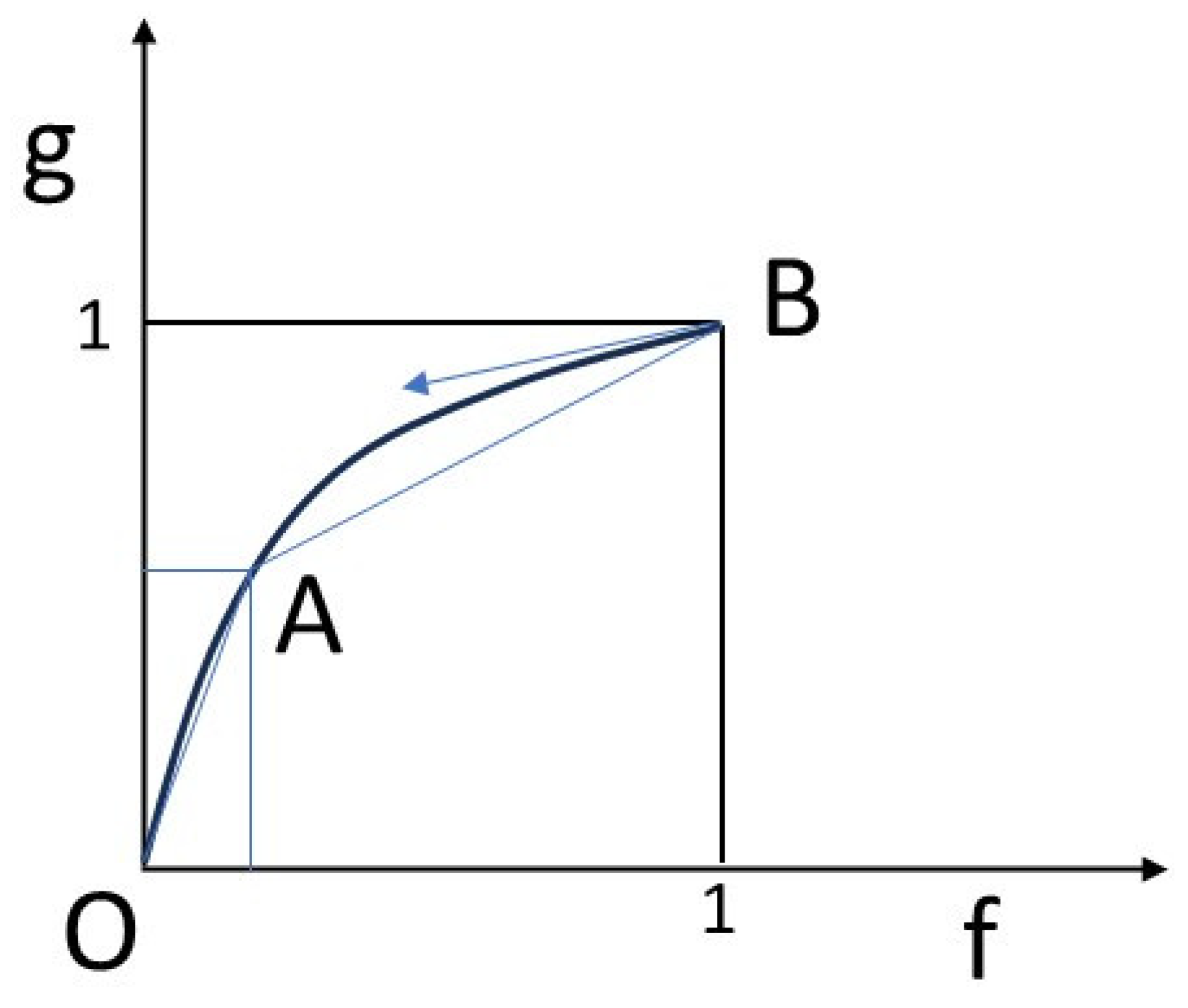
Figure 2.
Representation of the reactor studied. The reactor of finite length L is represented along the x-axis. The fluid enters from its left side at x = 0, and leaves to the right from x = L. The initial concentration in the fluid contained in the reactor (and along the x-axis) is g = 0, the incoming concentration at x = 0 is g = 1. The corresponding equilibrium concentrations for the solid are f = 0 and f = 1, respectively.
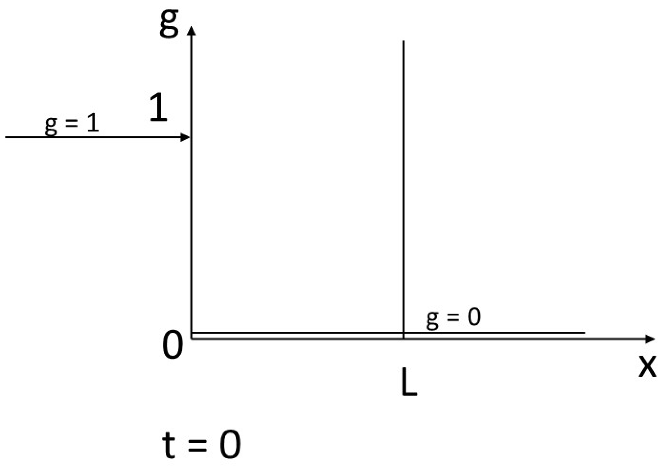
Figure 3.
Representation of the reactor crossed by two composition discontinuities. The state of the reactor at a given moment has been represented, traversed by a composition discontinuity leading from g = 0 to point A, followed by another discontinuity connecting point A to point B; points A and B are shown in Figure 1. Applying the rules governing velocities recalled in the caption of Figure 1, we can see that the velocity of the first front is almost six times faster than that of the second.
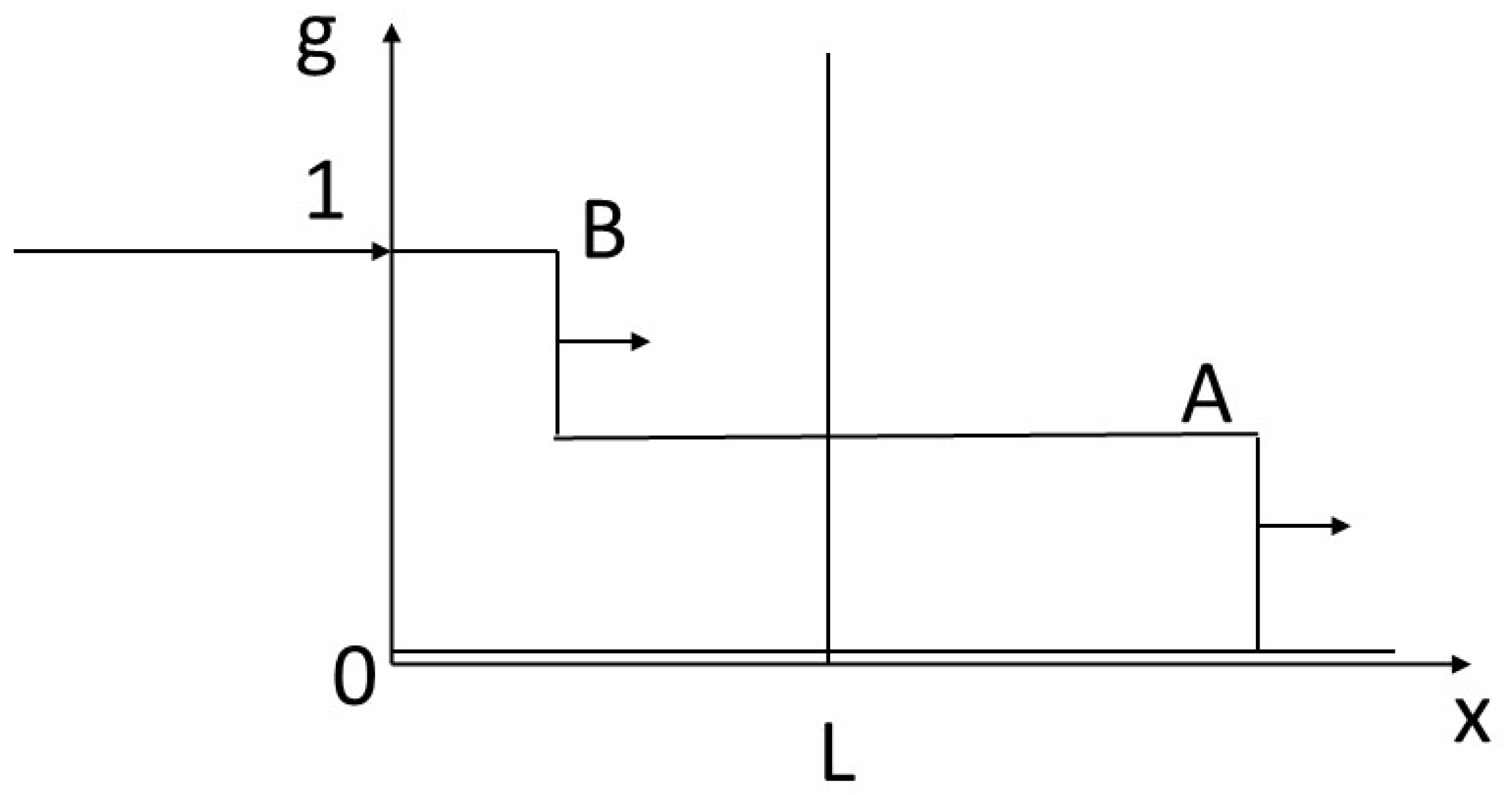
Figure 4.
Representation of the reactor pervaded by a shock and a détente. By comparison with the previous figure, the discontinuity between 0 and A is kept, but there is a détente between A and B. The advance velocity of B is given by the tangent to the isotherm at the corresponding point (see Figure 1).
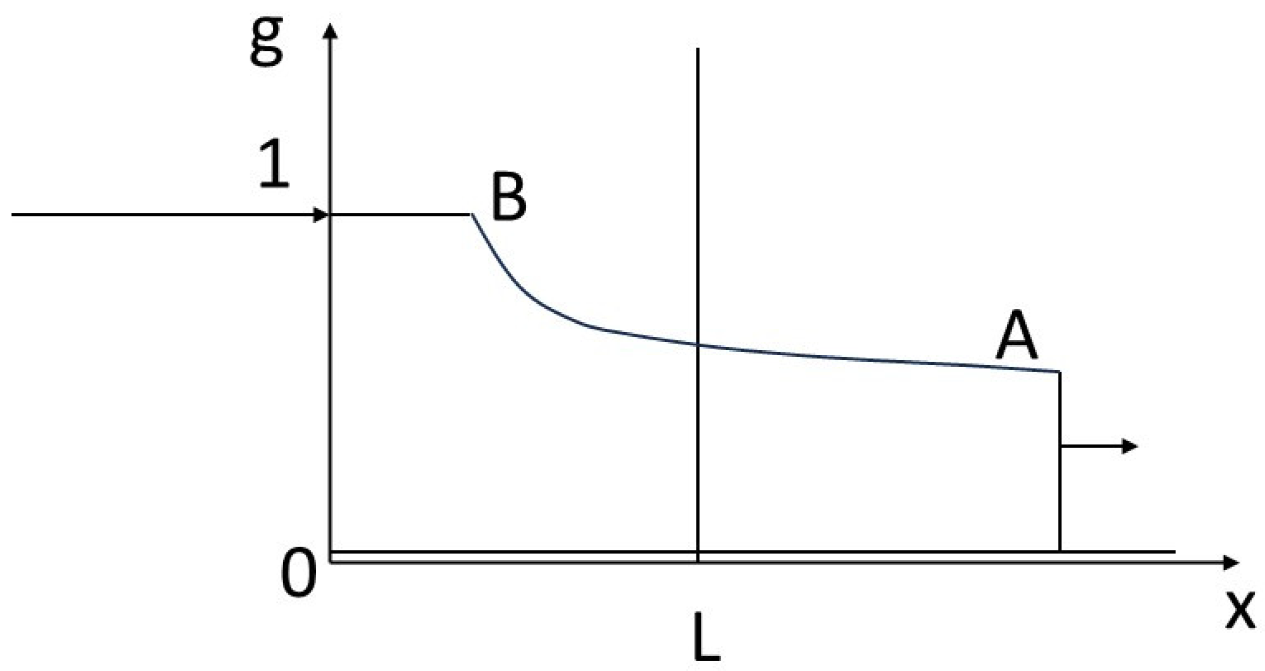
Figure 5.
Representation of a reactor traversed by a single shock. Here we have the case of a single discontinuity between point O (0, 0) and point B (1, 1) with a velocity equal to 1, i.e., the slope of the segment connecting the two points on the isotherm (Figure 1).
Figure 5.
Representation of a reactor traversed by a single shock. Here we have the case of a single discontinuity between point O (0, 0) and point B (1, 1) with a velocity equal to 1, i.e., the slope of the segment connecting the two points on the isotherm (Figure 1).
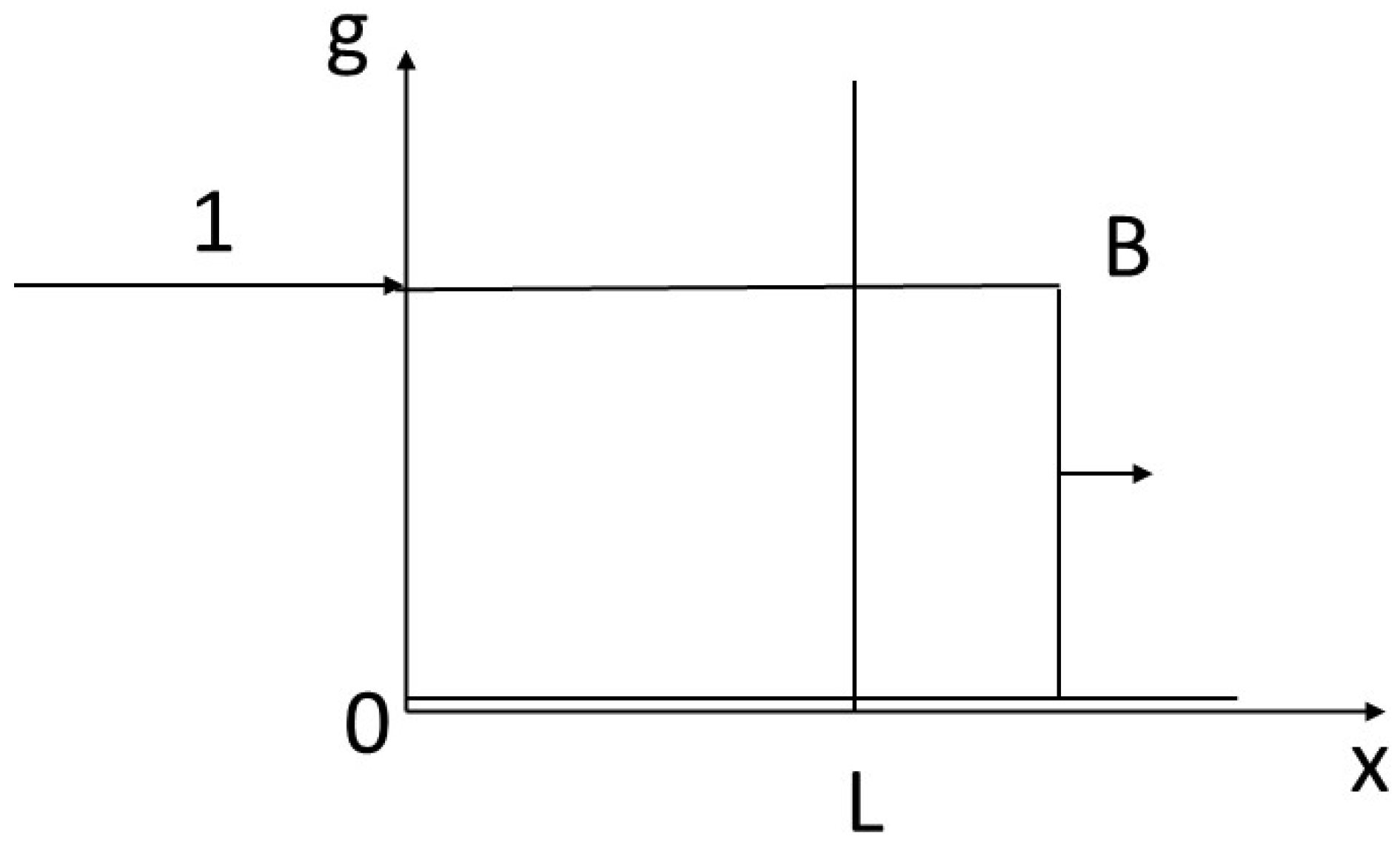
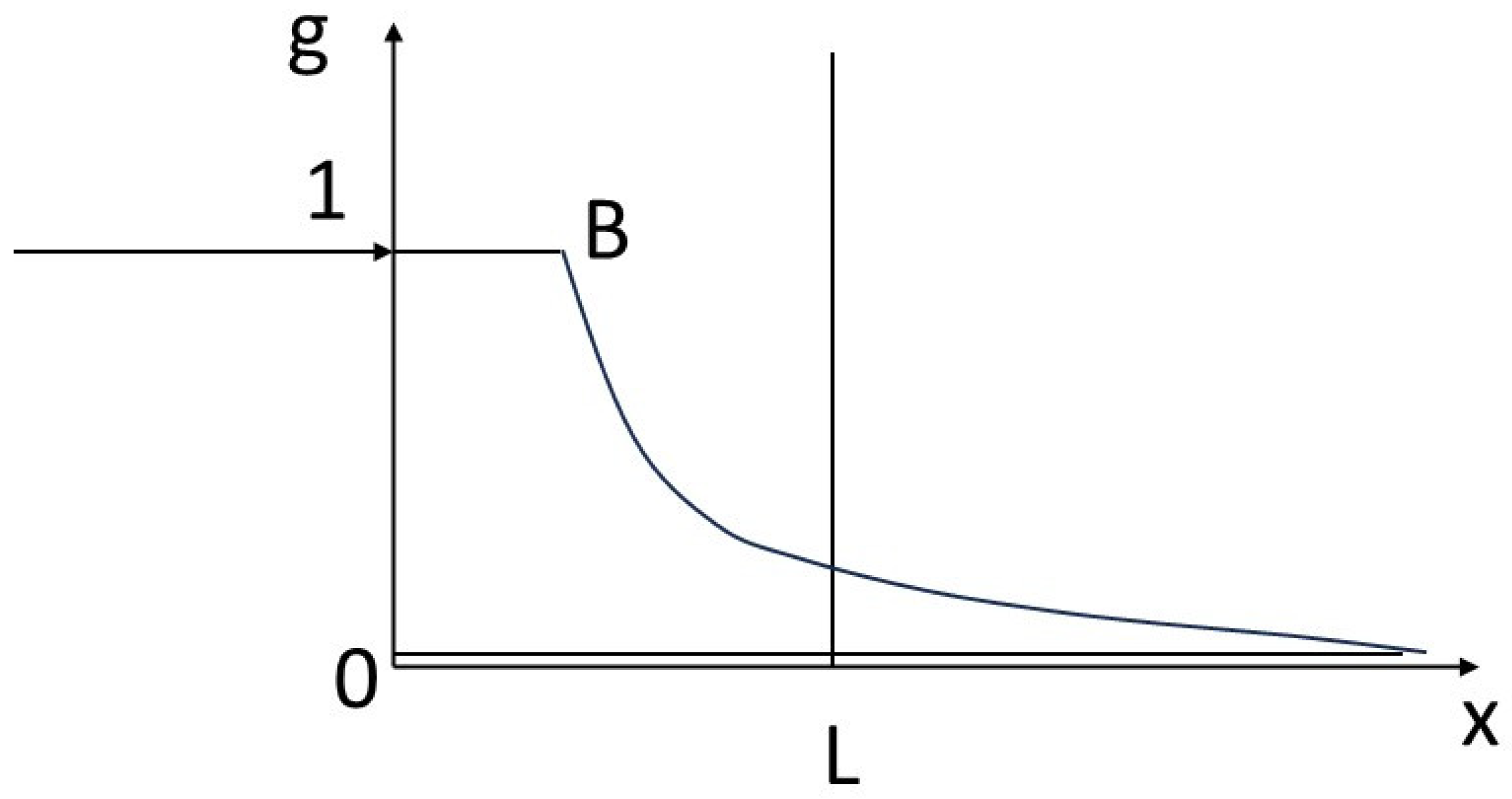
Figure 6.
Representation of the reactor through which a composition détente takes place. In contrast to Figures 3 to 5, the reactor here is traversed by a complete détente linking point (0, 0) and point (1, 1) of the isotherm (Figure 1). The first velocities (for the smallest concentrations), visible on the slopes of the isotherm, are faster than those for the largest concentrations, which arrive behind (lower slopes) and are therefore ahead, generating the détente. Only this configuration respects the entropy condition and makes physical sense.
Disclaimer/Publisher’s Note: The statements, opinions and data contained in all publications are solely those of the individual author(s) and contributor(s) and not of MDPI and/or the editor(s). MDPI and/or the editor(s) disclaim responsibility for any injury to people or property resulting from any ideas, methods, instructions or products referred to in the content. |
© 2025 by the authors. Licensee MDPI, Basel, Switzerland. This article is an open access article distributed under the terms and conditions of the Creative Commons Attribution (CC BY) license (http://creativecommons.org/licenses/by/4.0/).
Copyright: This open access article is published under a Creative Commons CC BY 4.0 license, which permit the free download, distribution, and reuse, provided that the author and preprint are cited in any reuse.


