
Submitted:
21 April 2025
Posted:
21 April 2025
Read the latest preprint version here
Abstract
In this paper, the author utilizes the frailty model to construct a new Archimedean copula. This copula depends on the transformed Median Based Unit Rayleigh (MBUR) distribution to unbounded distribution defined on the interval from zero to infinity. The copula only models the positive dependency. In the paper, the joint PDF and CDF of the copula are derived for two bivariate distributions. The singularity of the copula is explained. The generator and inverse generator of the new copula are explored with various graphs to depict the decreasing and convex nature of the generator with different dependency parameter values. The Kendall tau measure of dependency is derived. For this copula, the lower and upper tail dependencies exist. The formula for each one is derived. This new copula is one of the parametric Archimedean copulas. Unfortunately, the Archimedean copulas are not widely used.
Keywords:
Frailty model
; Archimedean copula
; generator
; inverse generator
; MBUR distribution
Introduction
A copula is a function mapping and satisfying the boundary condition in the form of , the unit marginal conditions in the form of , and 2-increasing property that states,
then,
and for , hence satisfying Lipschitz condition that is
Sklar (Sklar, 1973) showed that a copula exists for any multivariate distribution, such that the joint distribution equals the copula applied to the marginal. In other words, Let X and Y be random variables with joint distribution and marginal distribution functions and , respectively. Then there is a uniquely determined copula, C, on the , such that for . So copulas connect joint distributions functions to their margins. They are crucial for constructing bivariate and multivariate distributions because they are a statistical method for studying scale-free measures of dependence.
Definition 1
(Sklar’s theorem 1): For any bivariate distribution function H with marginal
and , there exists a copula such that
If H is continuous, then the copula C is unique. Otherwise, it is uniquely determined on the . The converse is also true, for any copula and univariate distribution functions and , the function is a bivariate distribution function with margins and .
Definition 2
: A bivariate Archimedean copula
can be written in the form of with marginal and , where is the generator function being continuous, strictly decreasing and convex function mapping onto , in other words, , decreasing) and (convex), , and → φ1=0
Definition 3
: a bivariate copula has which is the joint PDF of the copula.
So the copula links the marginal distributions through the dependency parameter.
The singular part of the copula is defined by (Genest & Mackay, 1986) in the following Theorem, the ratio between the generator and the first derivative of the generator evaluated at zero does not equal zero.
Theorem
: the distribution generated by has a singular component iff in that case, with probability =
In the last few years many models have been proposed for copulas. The applications of copulas are too plentiful to list so further improvements of copulas are encouraged to be further advanced. The applied applications rely mainly on the parametric models for copulas in comparison to the semi-parametric and non-parametric model for copulas which have limited applied implementations in real life.
Many eminent scientists and authors had in depth papers discussing the estimation methods, simulation, probabilistic interpretations, and analytical properties. Many problems face the statistical scientific community and in need for solutions. (Nadarajah et al., 2018) mentioned some of these problems like estimation of copula under misspecification, copula density estimation, Bayesian copula, change point estimation of copulas, efficient estimation and simulation algorithms, characterization of copulas, selection criteria between two or more copulas, time series models constructed on copulas, bounds for copulas, copula calibration, transformations to enhance fits of copulas, extreme value manners of bivariate and multivariate copulas, compatibility of copulas, additional measures of asymmetry for bivariate and multivariate copulas, extra tests for symmetry for bivariate and multivariate copulas, time varying copulas, space changing copulas and copulas fluctuating with sense of both time and space.
Many books had been written by pioneer and innovator scientists in the field of copulas like books written by (Drouet-Mari & Kotz, 2001), (Cuadras et al., 2002), (Cherubini et al., 2004), (Genest, 2005a), (Genest, 2005b), (Nelson, 2006), (McNeil et al., 2005), (Alsina et al., 2006), (Mai & Scherer, 2014), (Durante & Sempi, 2015), (Salvadori et al., 2007), (Malevergne & Sornette, 2006), (Schweizer & Sklar, 2005), (Jaworski et al., 2010),(Jaworski et al., 2013), (Joe, 2014), (Joe, 1997)and many others. Numerous papers had been published by many prominent scientists like (Nelsen, 2002), (Embrechts et al., 2003), (Manner & Reznikova, 2012), (Patton, 2012),(Genest et al., 2009),(Schweizer, 1991), (Kolev et al., 2006), (Kolev & Paiva, 2009), and (Frees & Valdez, 1998).
The copula can be grouped into five subgroups which are the Archimedean copulas, the elliptical copulas, the Eyraud-Farlie-Gumbel-Morgenstern (EFGM) copula, extreme value copulas, and other copulas. Each of these subgroups includes more copulas. For more details, the reader can be referred to the paper of (Nadarajah et al., 2018) and references therein.
The simplest copula is the product copula or the independence copula . It is for two independent random variables with . The other two very essential dependencies between two variables are the perfect positive and the perfect negative dependencies. These can be expressed by copulas. For the positive state, this yields . Hence, for random variables X and Y with distributions , and the joint distribution , and because the copula is symmetric, the random variable X is an increasing function of Y and vice versa. The converse, with decreasing instead of increasing holds true for the joint distribution function with . This one is also a copula. These boundaries are themselves copulas and they are called Frechet-Hoeffding upper and lower bound respectively. As long as both and are not differentiable in u and v, they have no density functions. Joe (Joe, 1990), (Joe & Hu, 1996), (Joe, 1993) developed copulas that allow for positive dependency only. These copulas are recently used in portfolio risk analysis with Asian equity markets (Ozun & Cifter, 2007).
This paper is structured in 6 sections. Section 1 discusses the methodology of derivation. section 2 illustrates the generator and its properties. Section 3 explores the inverse generator and its properties. Section 4 explains the Kendal Tau measure of dependency. Section 5 enlightens how the copula can model both lower and upper tail dependencies. Section 6 elucidates the final conclusions and future works. Numerous figures for its PDF and CDF are depicted.
1. Methodology of Derivation
This copula depends on the frailty method for generating the copula. Assuming two individuals have survival time distributed as exponential and . They have exponential baseline hazard function with . The survival function is shown in equation (1) and the hazard function in equation (2)
The Cox proportional hazard model uses the hazard function as shown in equation (3)
where the Z are the explanatory variables in survival analysis and b(t) is the baseline hazard function. And B is the vector of regression coefficients. It is proportional because all information is contained in the multiplicative factor , this is called the frailty model when some explanatory variables (Z) and hence the factor are unobserved. And the factor is called the frailty parameter. Integrating and exponentiating the negative hazard
for 2 explanatory variables for example
The marginal distribution for a single life time T is obtained by taking expectation over the potential values of that is , assuming the is the PDF of the frailty variable so
Let y be a random variable distributed as Median Based Unit Rayleigh (BMUR) (Attia, M.I., 2024), transform this variable to be defined on the interval from zero to infinity as shown below. The PDF of the Median Based Unit Rayleigh (MBUR) is shown in equation (4)
The following transformation will be applied to the above PDF:
Let
The Jacobian is shown in equation (5)
Replace the transformation of equation (5) into equation (4) as shown in equation (6):
Now this w is the frailty variable which is distributed as unbounded MBUR defined on the interval . Now take the conditional expectation of the survival function of the time distributed as exponential random variable with hazard rate equal one (scale parameter or lambda=1) given the frailty variable as shown in equation (7)
We can think of this expectation as a function of the frailty variable, it is averaging the probability to survive beyond specific time given that frailty. It is the expectation of a function of the frailty not the variable frailty itself so this function which is the baseline survival function should be multiplied by the PDF of the frailty variable. This way the frailty variable is integrated out. So this expectation is considered as the joint CDF of the two random variables T1 and T2. How to get this time? By inverting this expectation as shown in equation (8). Let us call this expectation u then solving second degree polynomial to get its root.
2. The Generator
In previous work by Iman M. Attia (Attia, 2025), the generator obtained by this method (modeling the frailty variable) yielded a Kendall tau measure that is fixed. As shown here the same method with different re-parameterization yielded a generator with no dependency parameter; therefore, the author did some manipulations to enhance the Kendall tau measures. The author added dependency parameter and remove the denominator as shown in the following equation (9), is the marginal CDF.
This (t) is the generator and (u) is the inverse generator. So the time (t) is a function of (u)
Preposition 1
: the generator shown in equation (9), can be considered as a generator for this new Archimedean copula.
Proof
: The generator fulfills the sufficient conditions of a generator.
- 1)
- 2)
- 3)
-
This ensures that the generator is a decreasing function in u.
- 4)
-
This ensures that the generator is a convex function atFor bivariate distribution with uniform marginal CDF (u) and (v), the generators are shown in equations (10-12)
3. The Inverse Generator
To get the inverse generator of this modified generator, the author inverts this (t) as shown in equation (13), as long as t equals:
Recall that
As a valid bivariate Archimedean copula can be expressed as
Proposition 2
: The copula expressed in equation (13) can be assumed to be a valid copula as it fulfills the boundary conditions, the marginal uniformity and 2- increasing conditions. And this is equivalent to the necessary conditions of the inverse generator to be fulfilled which are the following:
Proof:
, boundary conditions are fulfilled
, the marginal uniformity, when u=1
The same is true for v, if v=1 so
Proposition 3
: This is a valid copula as it is 2-increasing, i.e.,
in equation (14)
Proof:
Let
Proposition 4
: This copula is absolutely continuous copula and it has no singular part.
Proof:
to test for singularity: in equation (15). If this limit is zero so the copula has no singular part.
As long as this limit is zero at u=0 so the copula has no singular part and it is absolutely continuous copula.
4. Kendall Tau Measure of Dependency
Proposition 5
: Kendall tau for this copula is
in equation (16)
Proof:
For this copula, new one can be created using the following pattern for the generator:
Let the so other generators can be created and hence related new copulas for each generator such as:
But the Kendall Tau measure of dependency calculation will be
For large values of the first part of integration will converge to and when added to the second part, the final result will converge to , when h attains large values so the Kendall tau measure of dependency will be
for large values of
Figure 1, Figure 2, Figure 3, Figure 4, Figure 5, Figure 6, Figure 7, Figure 8, Figure 9, Figure 10, Figure 11, Figure 12, Figure 13, Figure 14, Figure 15, Figure 16, Figure 17, Figure 18, Figure 19, Figure 20, Figure 21, Figure 22, Figure 23, Figure 24, Figure 25, Figure 26, Figure 27, Figure 28, Figure 29 and Figure 30 illustrate the joint PDF, the joint CDF and the related generator for the copula with different values of dependency parameter.
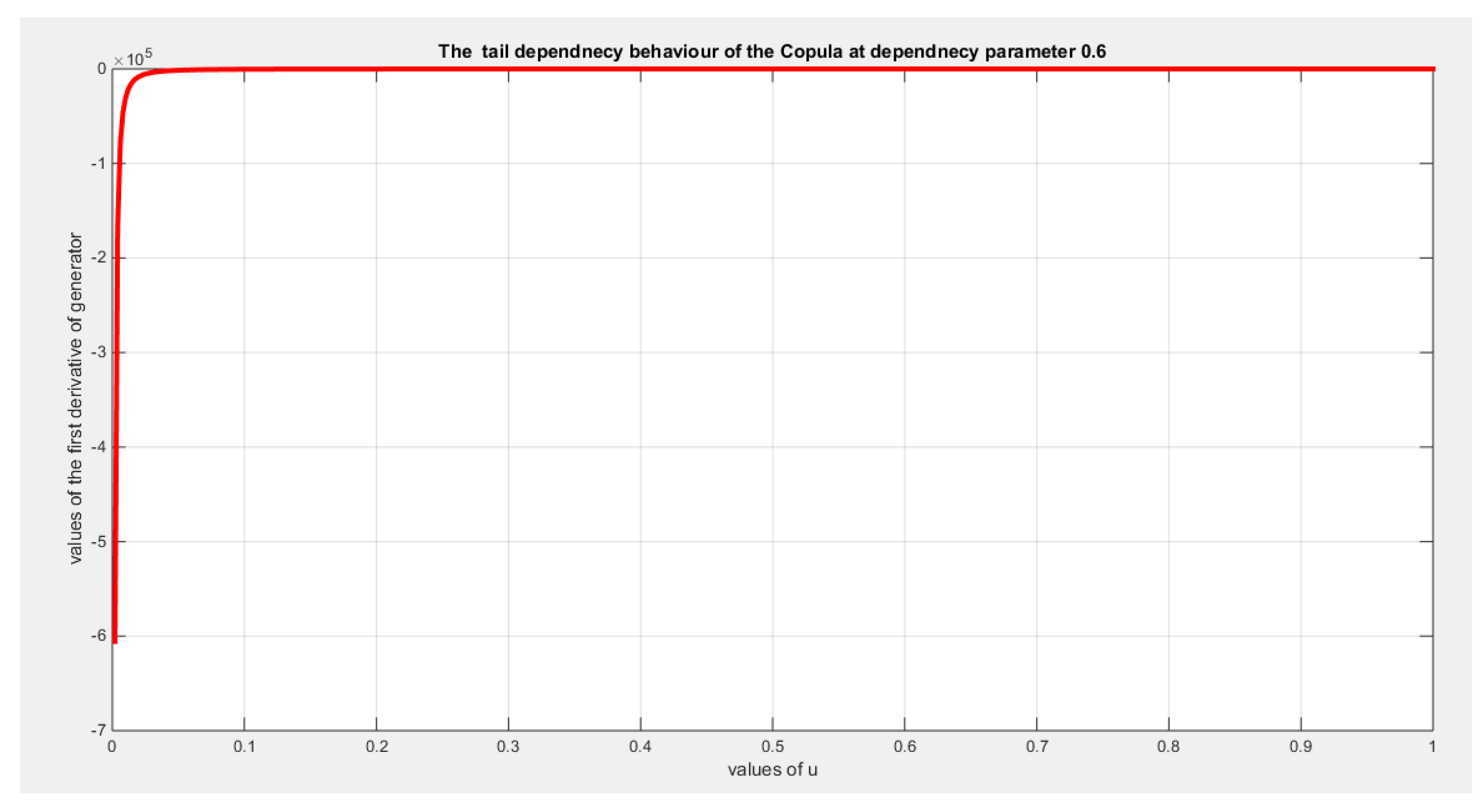
5. Tail Dependency
Preposition 6:
Lower and upper tail dependencies for this copula exist.
Proof:
Since both limits in equation (17-18) are infinite and as illustrated in Figure 3) so both lower and upper tail dependencies exist. Moreover, as shown in equation (19) and in Figure 32 the first derivative of the generator approaches at so the upper tail dependency exists.
Preposition 7
: The values of lower and upper tail dependency can be calculated as shown in equations (20-21)
Proof:
Lower tail dependency:
Upper tail dependency
As long as u is small
6. Conclusions
This copula which is based on frailty model and cox proportional hazard model can only model positive dependency. These types of copula can be used in applications to model the positive dependency between variables. This copula can also model lower and upper tail dependency. This copula has a generator whose derivative is zero when evaluated at zero and this supports modeling upper tail dependency. The definitions of lower and upper tail dependencies that involve the copula equation yielded infinite values and this also supports the tail dependencies.
While the joint distribution function, for two random variables X and Y, the bivariate density function these 2 variables is shown in equation (22)
Future Works
More works are needed to develop efficient estimation and simulation algorithms. Also Bayesian estimation can be used to enhance the estimation procedures. The copula can also be tested for some of the problems mentioned earlier in the introduction.
Author Contributions
AI carried the conceptualization by formulating the goals, aims of the research article, formal analysis by applying the statistical, mathematical and computational techniques to synthesize and analyze the hypothetical data, carried the methodology by creating the model, software programming and implementation, supervision, writing, drafting, editing, preparation, and creation of the presenting work.
Funding
No funding resource. No funding roles in the design of the study and collection, analysis, and interpretation of data and in writing the manuscript are declared
Ethics Approval and Consent to Participate
Not applicable.
Consent for Publication
Not applicable
Data Availability Statement
Not applicable. Data sharing not applicable to this article as no datasets were generated or analyzed during the current study.
Conflicts of Interest
The author declares no competing interests of any type.
References
- Alsina, C. Franks, M. F., & Schweizer, B. (2006). Associative Functions.Triangular Norms and Copulas. World Scientific, Singapore.
- Attia, I. M. (2025). New Three Different Generators for Constructing New Three Different Bivariate Copulas. Preprint.org. [CrossRef]
- Attia, M.I. (2024). A Novel Unit Distribution Named as Median Based Unit Rayleigh (MBUR):Properties and Estimations. Preprints.Org, Preprint, 7 October 2024(7 October 2024). [CrossRef]
- Cherubini, U. Luciano, E., & Vecchiato, W. (2004). Copula Methods In Finance. John Wiley and Sons.
- Cuadras, C. M. , Fortiana, J., & Rodriguez-Lallena, J. A. (2002). Distributions with Given Marginals and Statistical Modellings. Kluwer. Distributions with Given Marginals and Statistical Modellings.
- Drouet-Mari, D. , & Kotz, S. (2001). Correlation and Dependence. Imperial College Press.
- Durante, F. , & Sempi, C. (2015). Principles of Copula Theory. CRC Press.
- Embrechts, P. Lindskog, F., & Mcneil, A. (2003). Modelling Dependence with Copulas and Applications to Risk Management. In Handbook of Heavy Tailed Distributions in Finance (pp. 329–384). Elsevier. [CrossRef]
- Frees, E. W. , & Valdez, E. A. Understanding Relationships Using Copulas. North American Actuarial Journal 1998, 2, 1–25. [Google Scholar] [CrossRef]
- Genest, C. (2005a). Preface (Vol. 33). Candian Journal of statistics.
- Genest, C. (2005b). Preface (Vol. 37). Insurance: Mathematics and Economics.
- Genest, C. , & Mackay, J. The Joy of Copulas: Bivariate Distributions with Uniform Marginals. The American Statistician 1986, 40, 280–283. [Google Scholar] [CrossRef]
- Genest, C. , Rémillard, B., & Beaudoin, D. Goodness-of-fit tests for copulas: A review and a power study. Insurance: Mathematics and Economics 2009, 44, 199–213. [Google Scholar] [CrossRef]
- Jaworski, P. , Durante, F., & Hardle, W. (2013). Copula in Mathematical and Quantitative Finance. Springer Verlag.
- Jaworski, P. , Durante, F., Hardle, W., & Rychlik, T. (2010). Copula Theory and Its Applications: Proceedings of the Workshop held in Warsaw. (Lecture Notes in Statistics, Vol. 198). Springer Verlag.
- Joe, H. Families of min-stable multivariate exponential and multivariate extreme value distributions. Statistics & Probability Letters 1990, 9, 75–81. [Google Scholar] [CrossRef]
- Joe, H. Parametric Families of Multivariate Distributions with Given Margins. Journal of Multivariate Analysis 1993, 46, 262–282. [Google Scholar] [CrossRef]
- Joe, H. (1997). Multivariate Models and Dependence Concepts. Chapman and Hall.
- Joe, H. (2014). Dependence Modeling with Copulas. CRC Press.
- Joe, H. , & Hu, T. Multivariate Distributions from Mixtures of Max-Infinitely Divisible Distributions. Journal of Multivariate Analysis 1996, 57, 240–265. [Google Scholar] [CrossRef]
- Kolev, N. , Anjos, U. D., & Mendes, B. V. D. M. Copulas: A Review and Recent Developments. Stochastic Models 2006, 22, 617–660. [Google Scholar] [CrossRef]
- Kolev, N. , & Paiva, D. Copula-based regression models: A survey. Journal of Statistical Planning and Inference 2009, 139, 3847–3856. [Google Scholar] [CrossRef]
- Mai, J. F. & Scherer, M. (2014). Finanial Engineering with Copula Explained. Palgrave Macmillan.
- Malevergne, Y. , & Sornette, D. (2006). Extreme Financial Risks: From Dependence to Risk Management. Springer Verlag.
- Manner, H. , & Reznikova, O. A Survey on Time-Varying Copulas: Specification, Simulations, and Application. Econometric Reviews 2012, 31, 654–687. [Google Scholar] [CrossRef]
- McNeil, A. J. , Frey, R., & Embrechts, P. (2005). Quantitative Risk Management: Concepts, Techniques and Tools. Princeton University Press.
- Nadarajah, S. , Afuecheta, E., & Chan, S. A Compendium of Copulas. Statistica 2018, 77, 279–328. [Google Scholar] [CrossRef]
- Nelsen, R. B. (2002). Concordance and Copulas: A Survey. In C. M. Cuadras, J. Fortiana, & J. A. Rodriguez-Lallena (Eds.), Distributions With Given Marginals and Statistical Modelling (pp. 169–177). Springer Netherlands. [CrossRef]
- Nelson, R. B. (2006). An Introduction to Copulas. Springer Verlag.
- Ozun, A. , & Cifter, A. Estimating Portfolio Risk with Conditional Joe-Clayton Copula: An Empirical Analysis with Asian Equity Markets The IUP Journal of Financial Economics 2007, 28–41.
- Patton, A. J. A review of copula models for economic time series. Journal of Multivariate Analysis 2012, 110, 4–18. [Google Scholar] [CrossRef]
- Salvadori, G. , Michele, C. D., Kottegoda, N. T., & Rosso, R. (2007). Extremes in nature. An approach Using Copulas. Springer Verlag.
- Schweizer, B. (1991). Thirty Years of Copulas. In G. Dall’Aglio, S. Kotz, & G. Salinetti (Eds.), Advances in Probability Distributions with Given Marginals (pp. 13–50). Springer Netherlands. [CrossRef]
- Schweizer, B. , & Sklar, A. (2005). Probabilistic Metric Space. Dover, Mineola.
- Sklar, A. Random Variables, Joint distribution functions, and copulas. Kybernetika 1973, 9, 449–460. [Google Scholar]
Figure 1.
shows the generator function (decreasing and convex) at theta = 0.3.
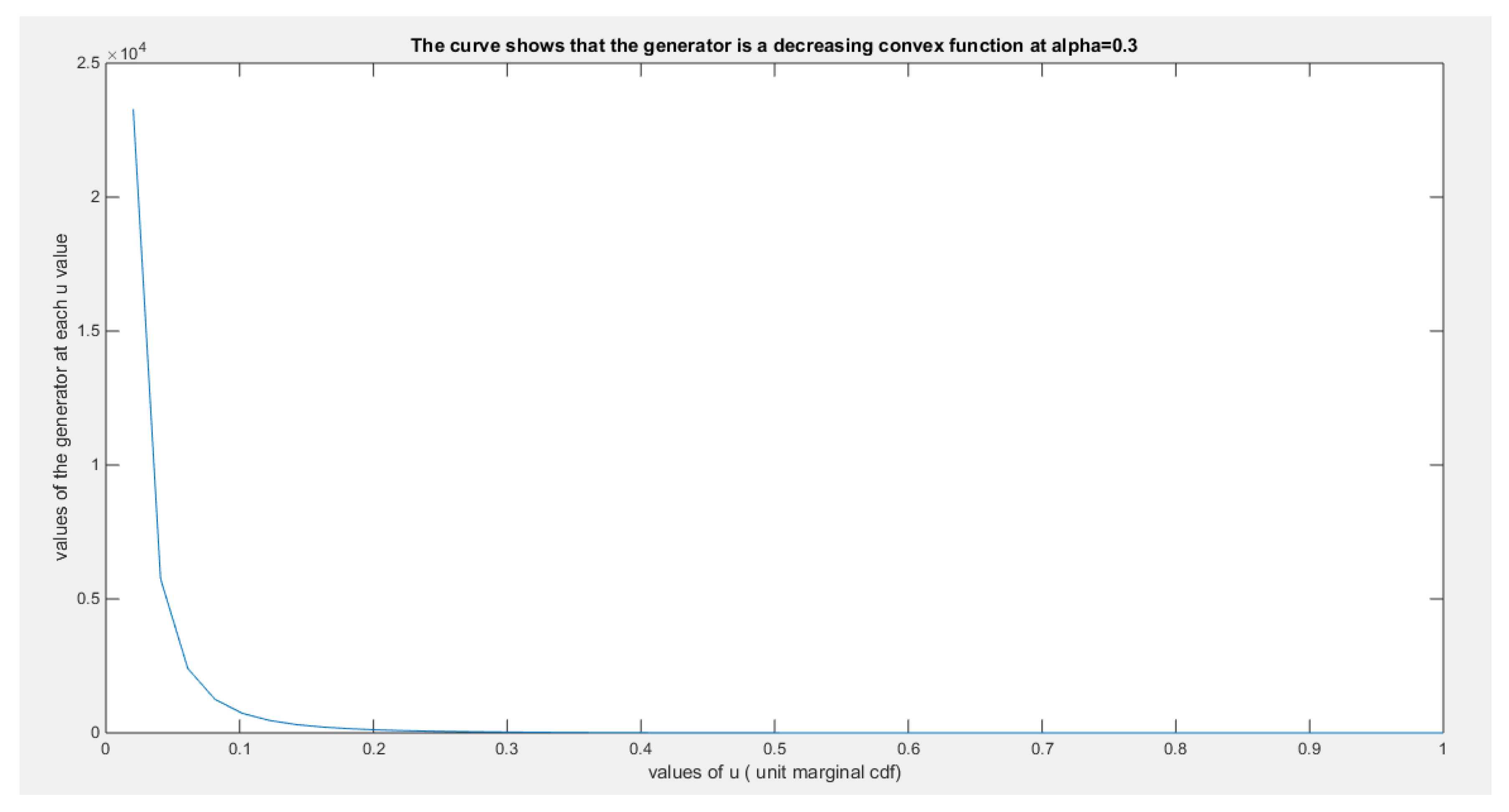
Figure 2.
shows the joint CDF copula (Copula) at theta = 0.3.
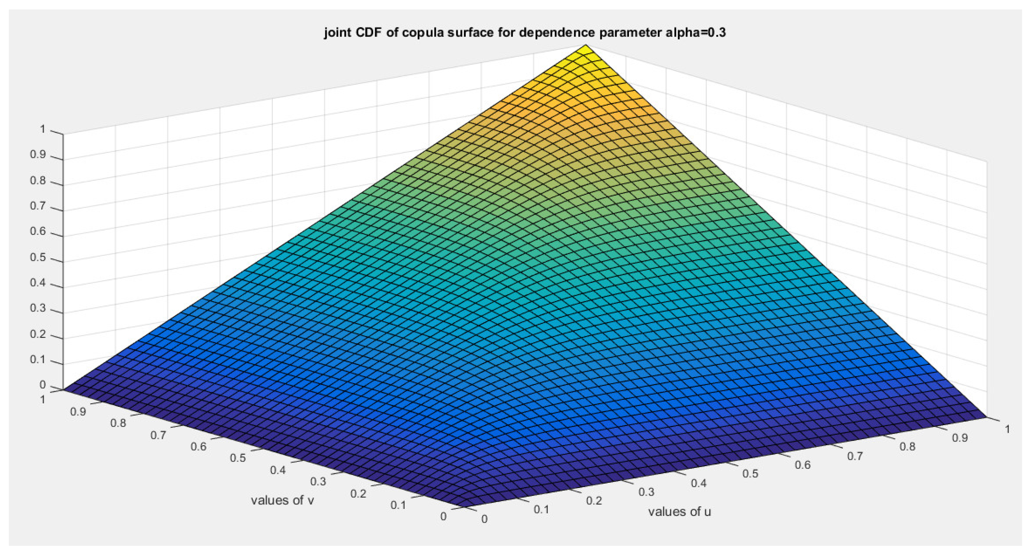
Figure 3.
shows the joint PDF copula (copula density) at theta = 0.3.
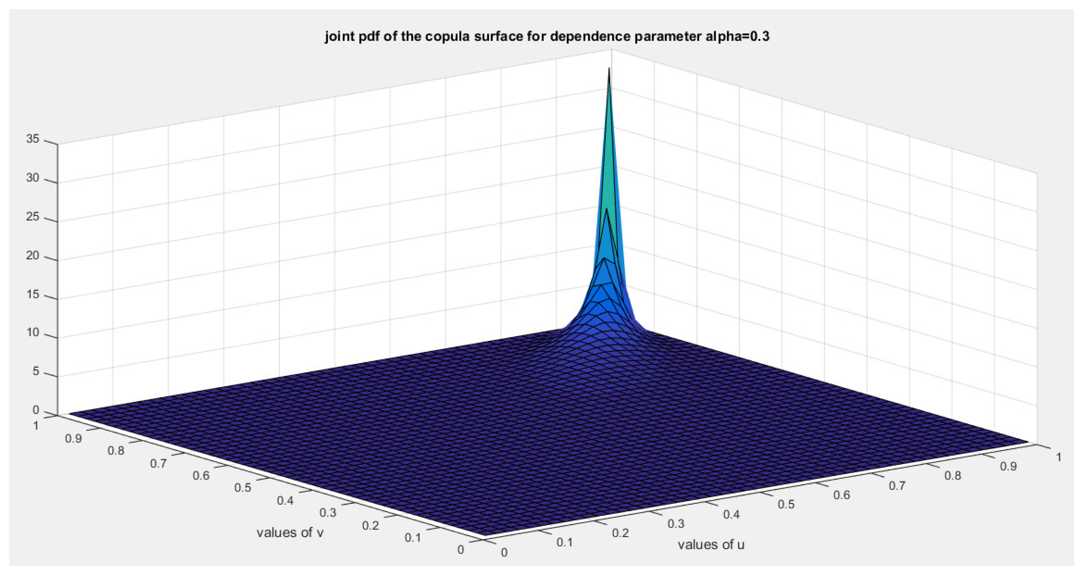
Figure 4.
shows the generator function (decreasing and convex) at theta = 0.6.
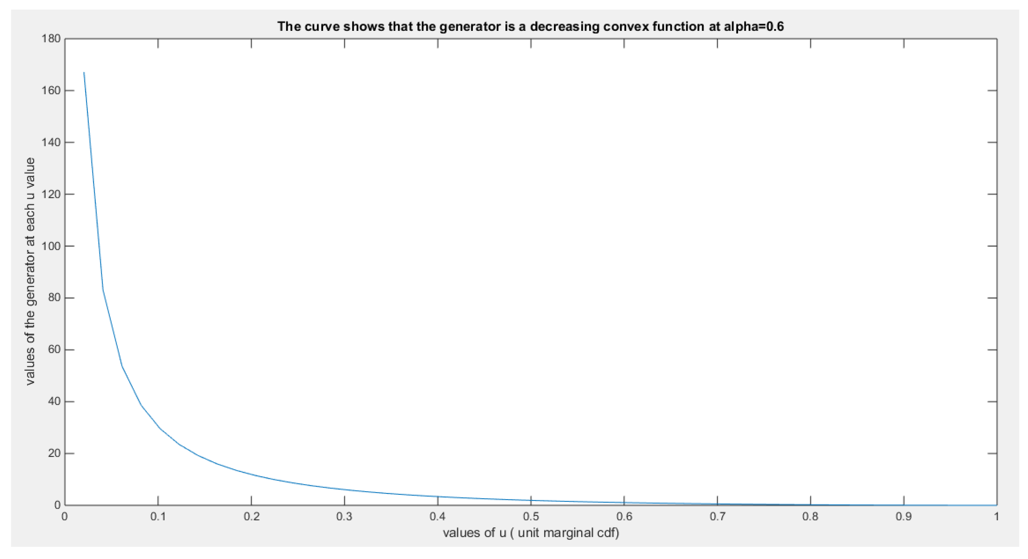
Figure 5.
shows the joint CDF copula (Copula) at theta = 0.6.
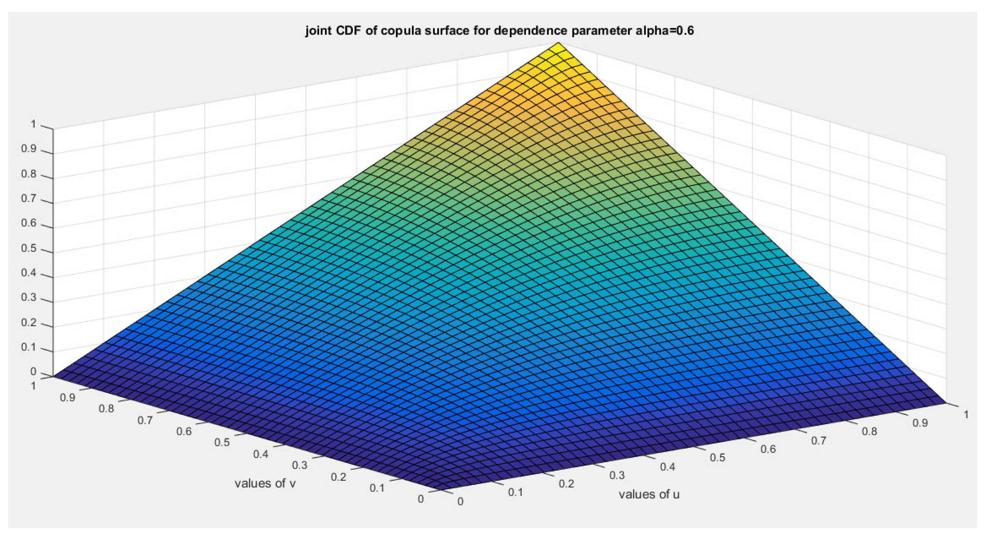
Figure 6.
shows the joint PDF copula (copula density) at theta = 0.6.
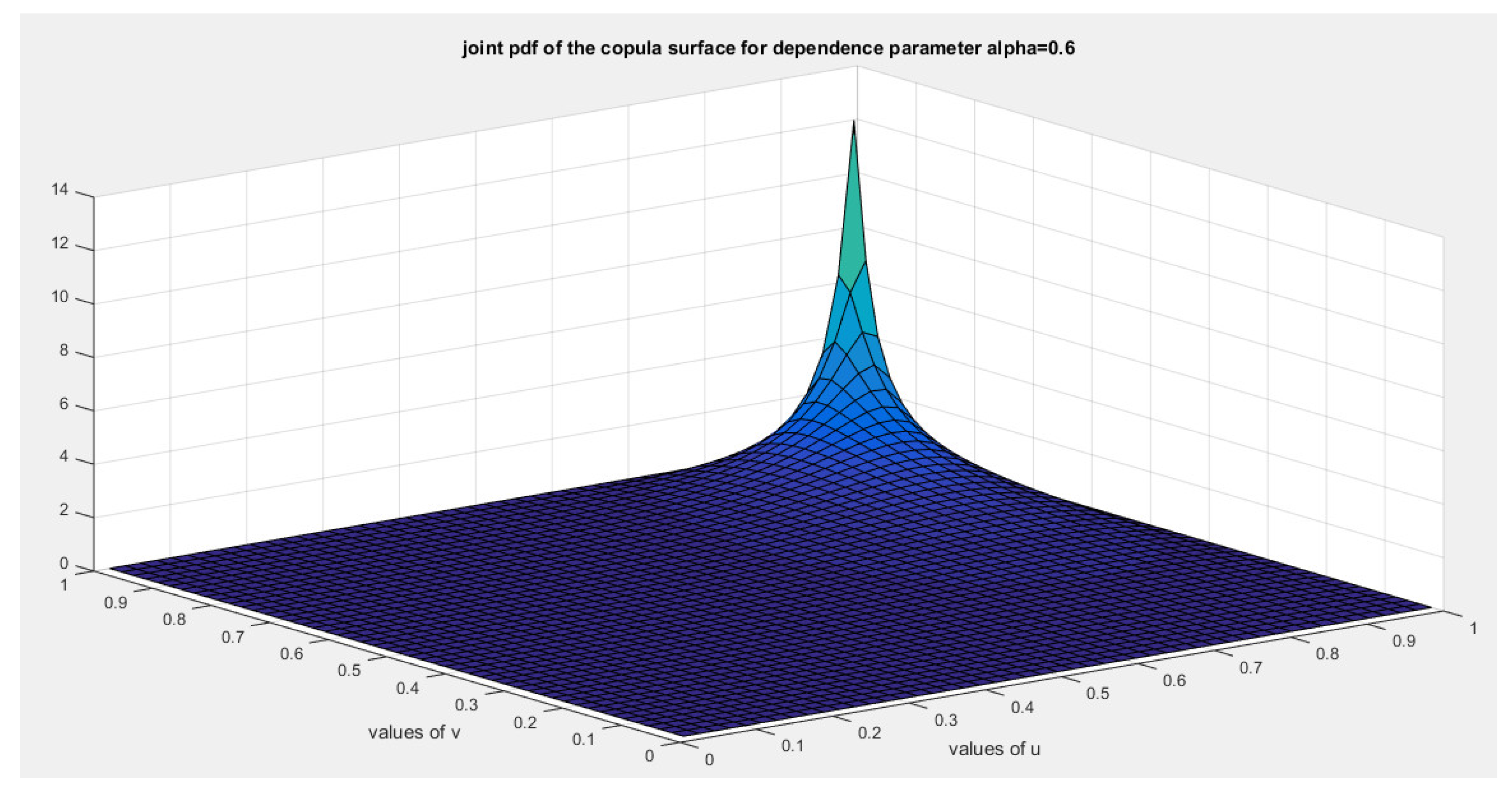
Figure 7.
shows the generator function (decreasing and convex) at theta = 0.888.
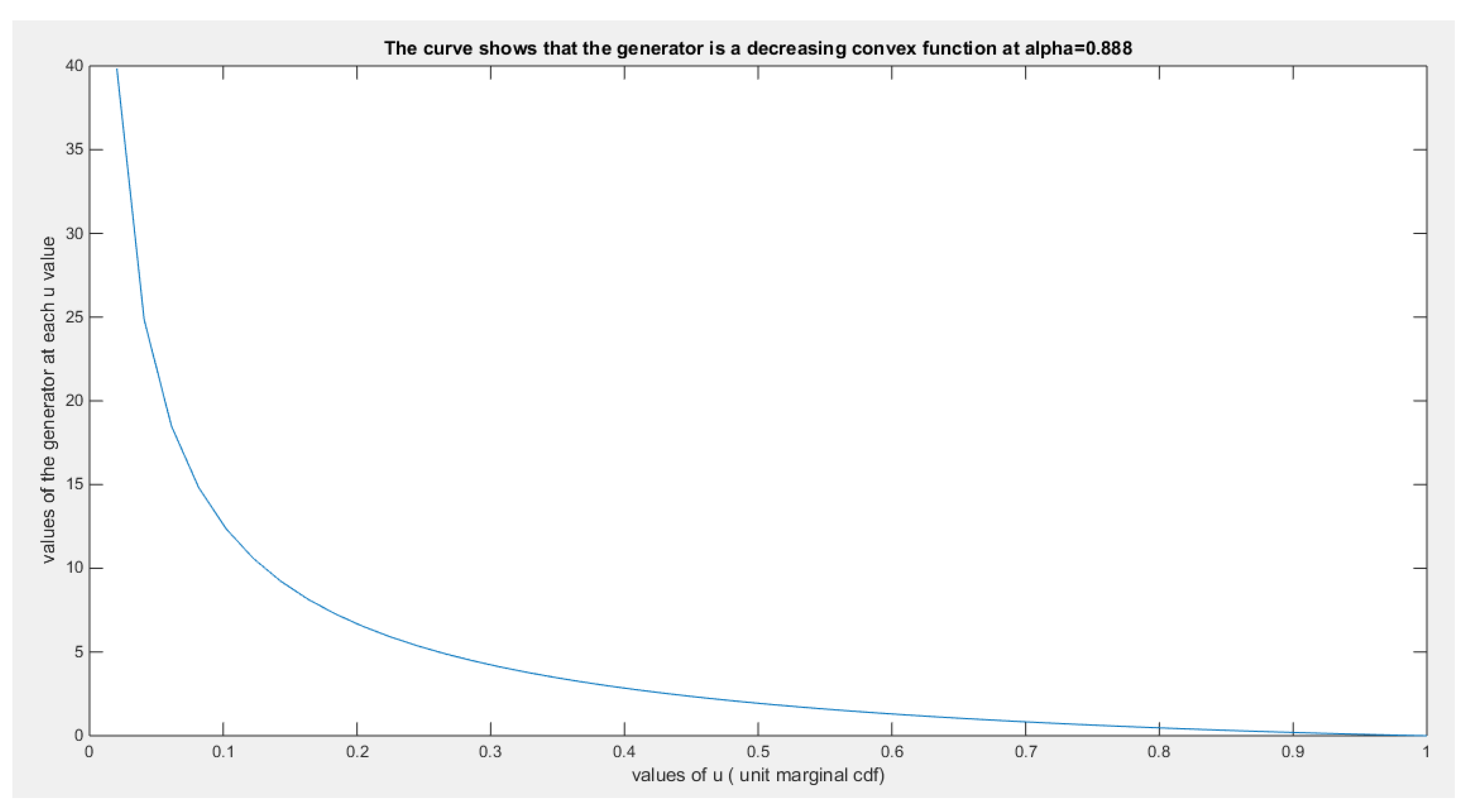
Figure 8.
shows the joint CDF copula (Copula) at theta = 0.888.
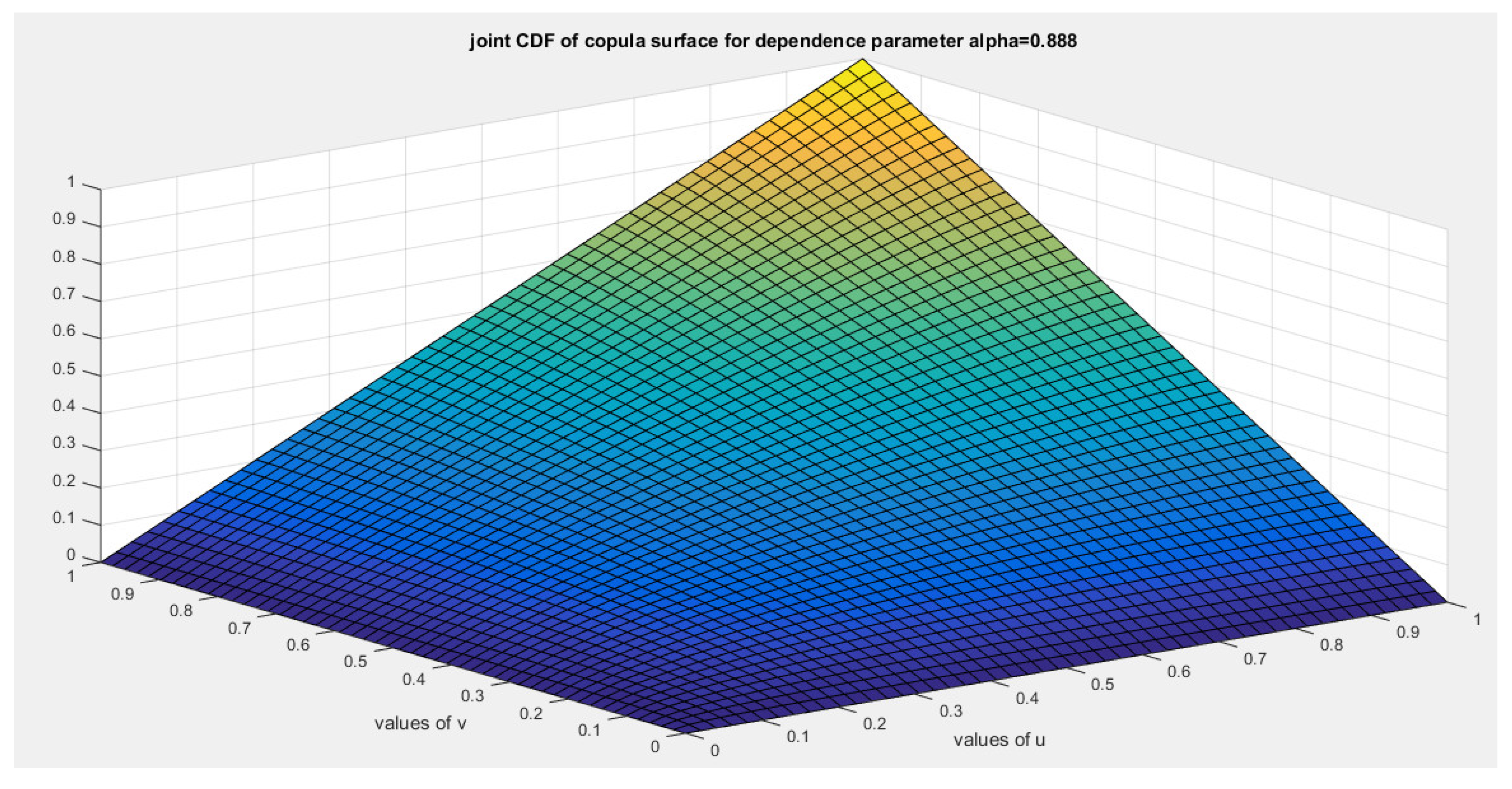
Figure 9.
shows the joint PDF copula (copula density) at theta = 0.888.
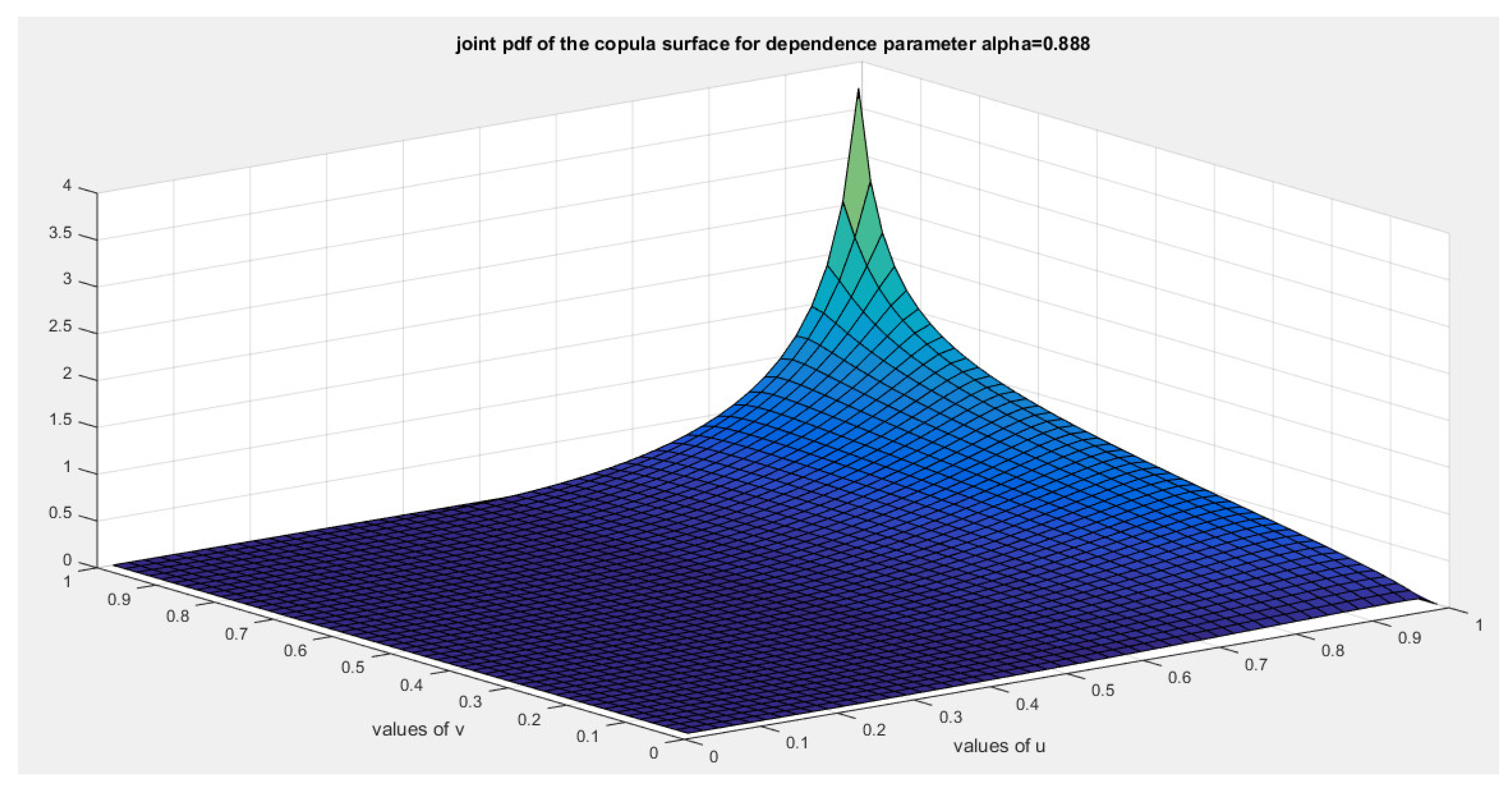
Figure 10.
shows the generator function (decreasing and convex) at theta = 0.999.
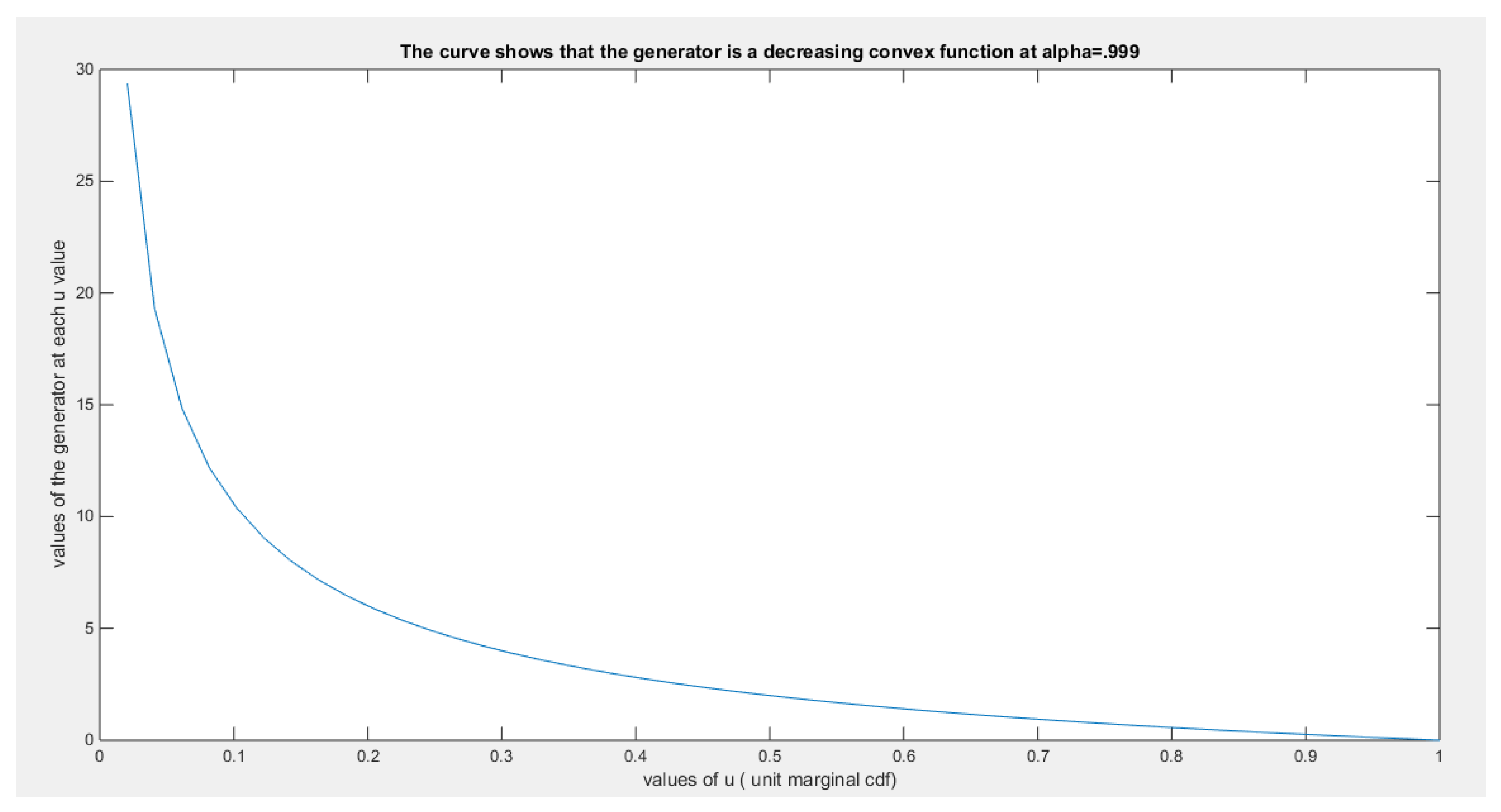
Figure 11.
shows the joint CDF copula (Copula) at theta = 0.999.

Figure 12.
shows the joint PDF copula (copula density) at theta = 0.999.
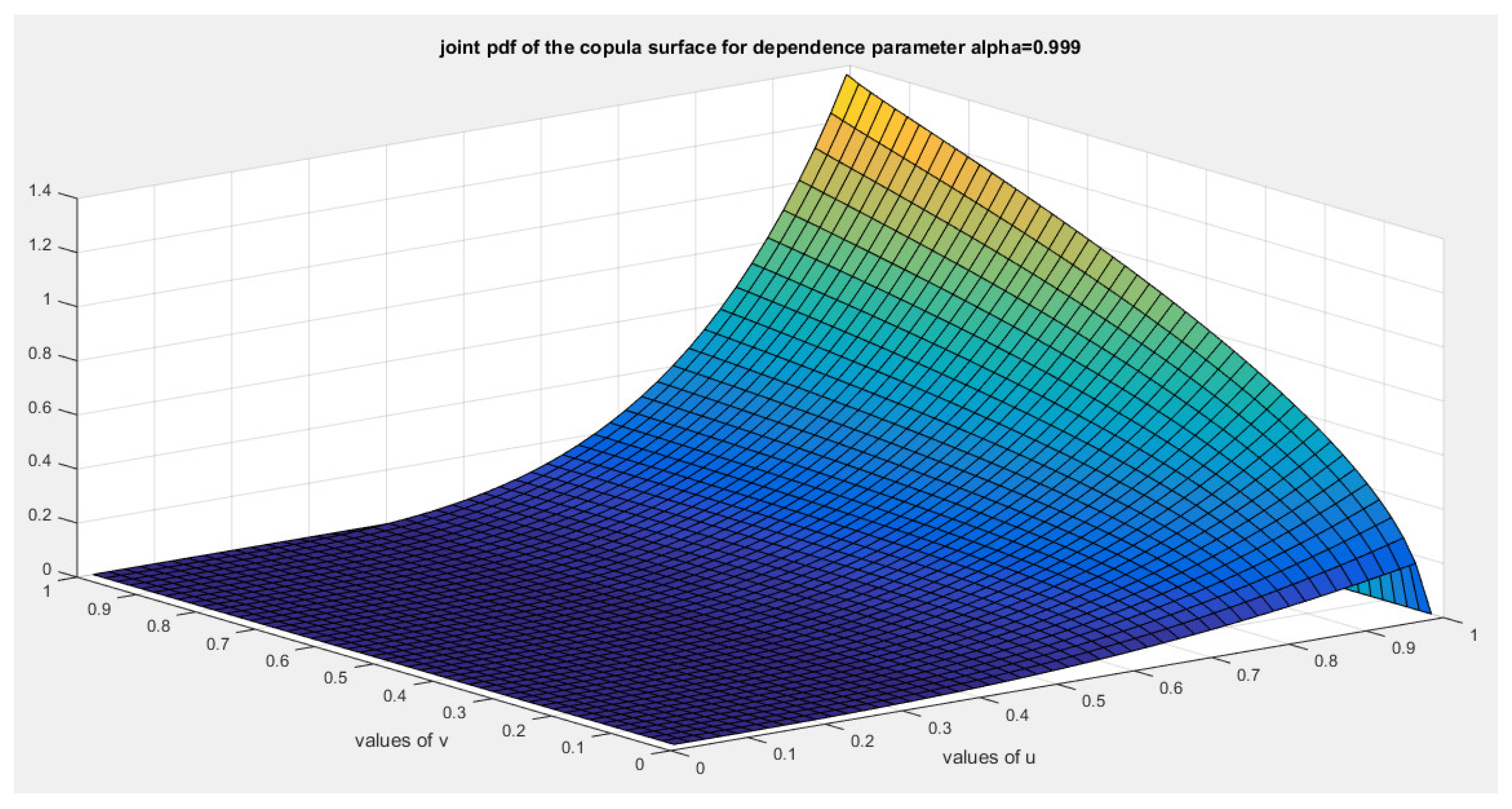
Figure 13.
shows the generator function (decreasing and convex) at theta = 1.
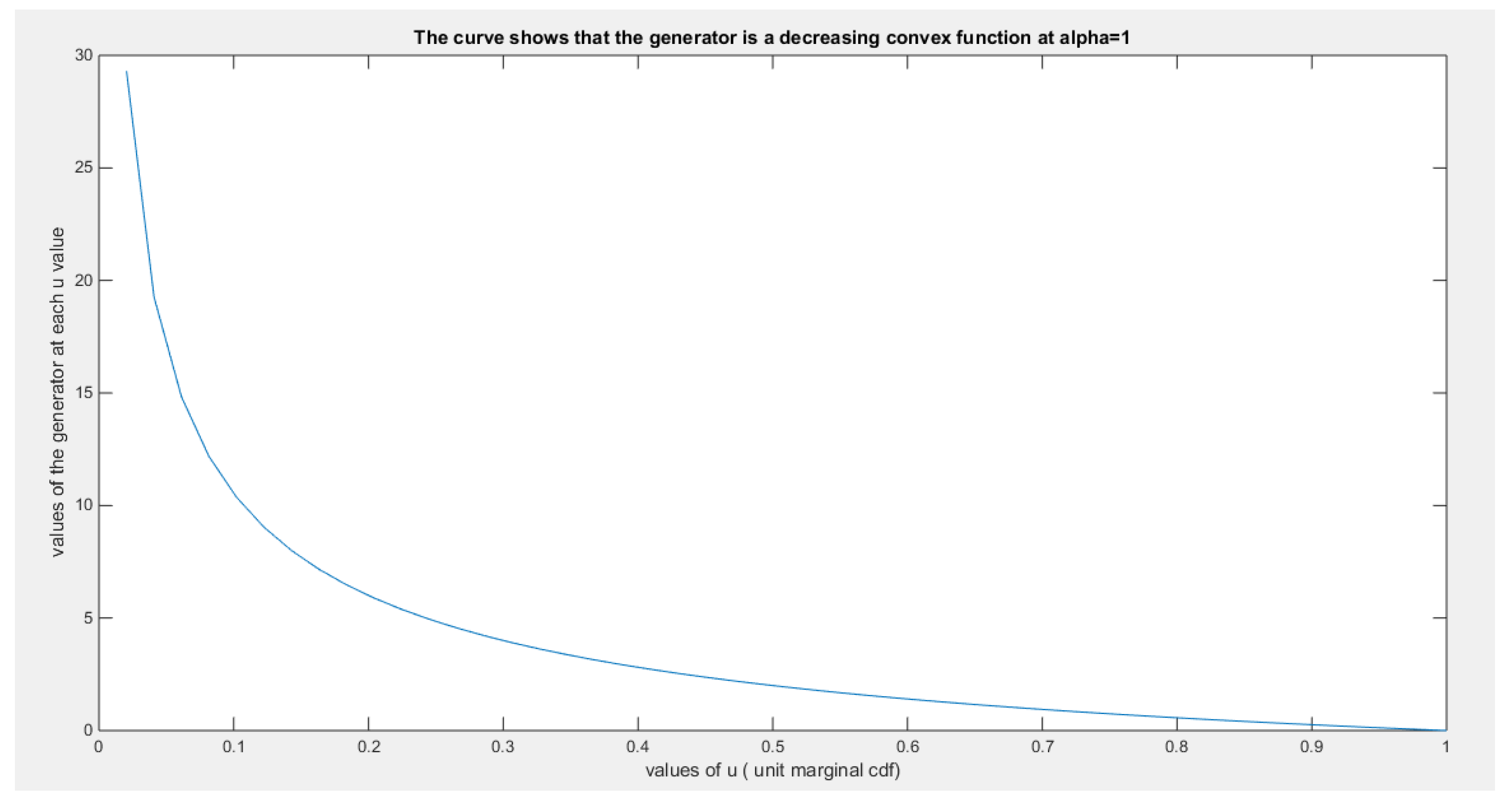
Figure 14.
shows the joint CDF copula (Copula) at theta = 1.
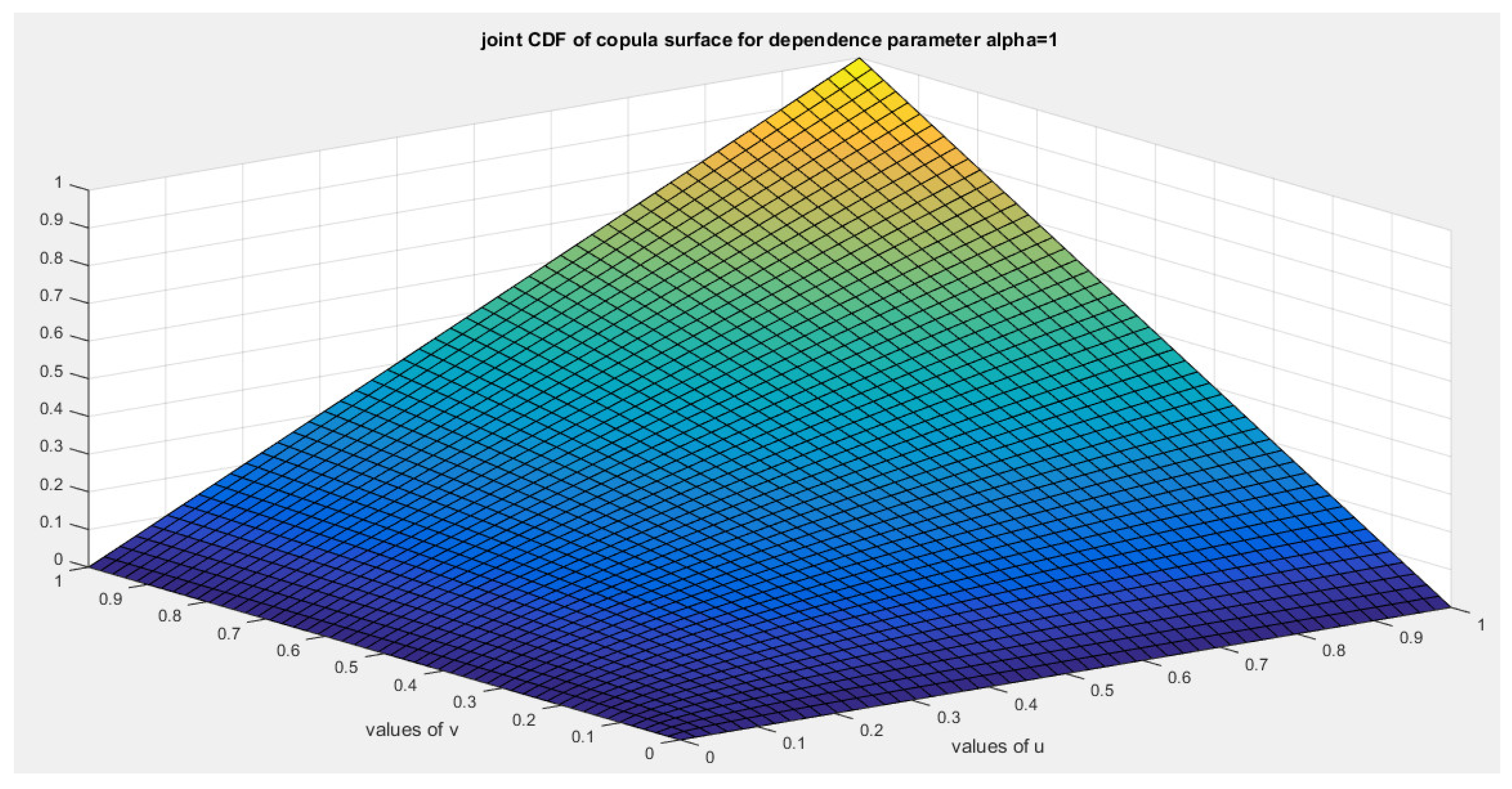
Figure 15.
shows the joint PDF copula (copula density) at theta = 1.

Figure 16.
shows the joint CDF copula (Copula) at theta = 0.001.
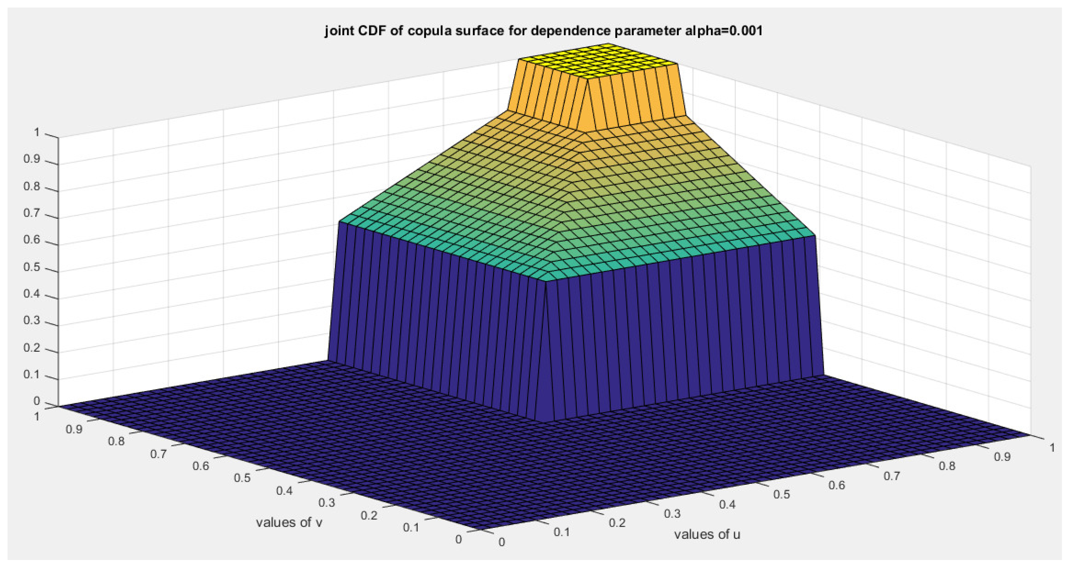
Figure 17.
shows the joint PDF copula at theta = 0.001.

Figure 18.
shows the joint CDF copula (Copula) at theta = 0.002.
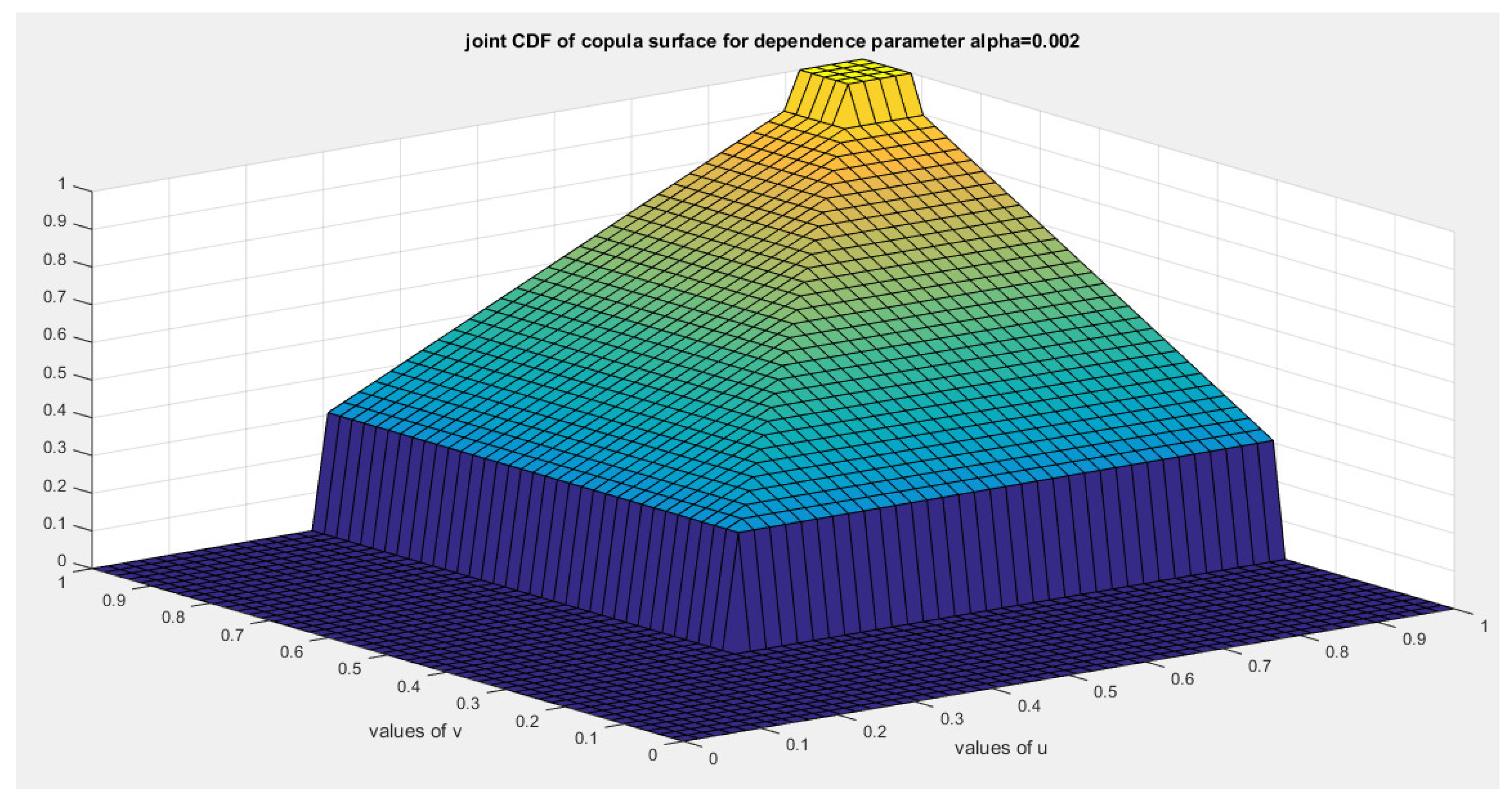
Figure 19.
shows the joint PDF copula at theta = 0.002.

Figure 20.
shows the joint CDF copula (Copula) at theta = 0.003.
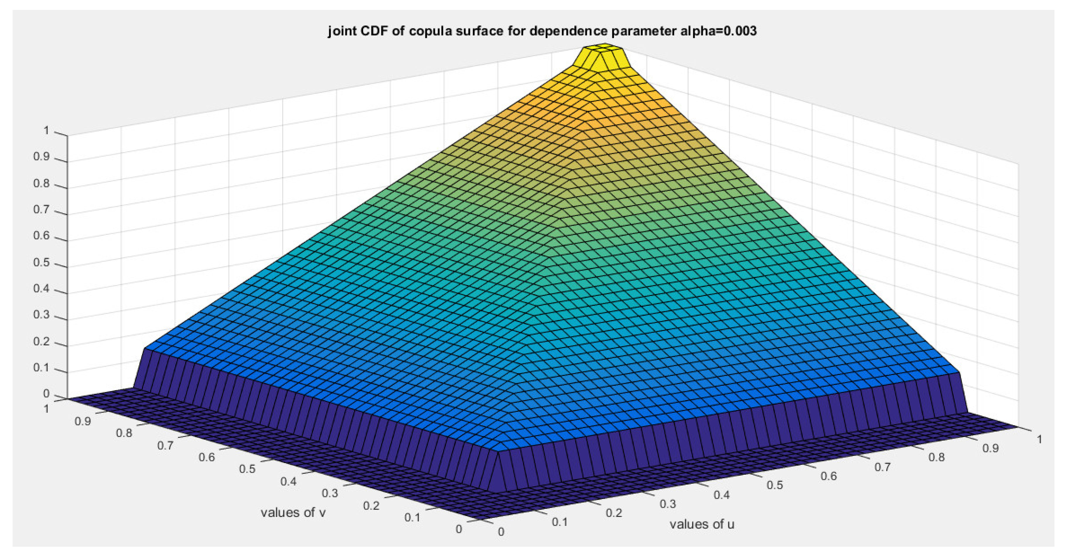
Figure 21.
shows the joint PDF copula at theta = 0.003.
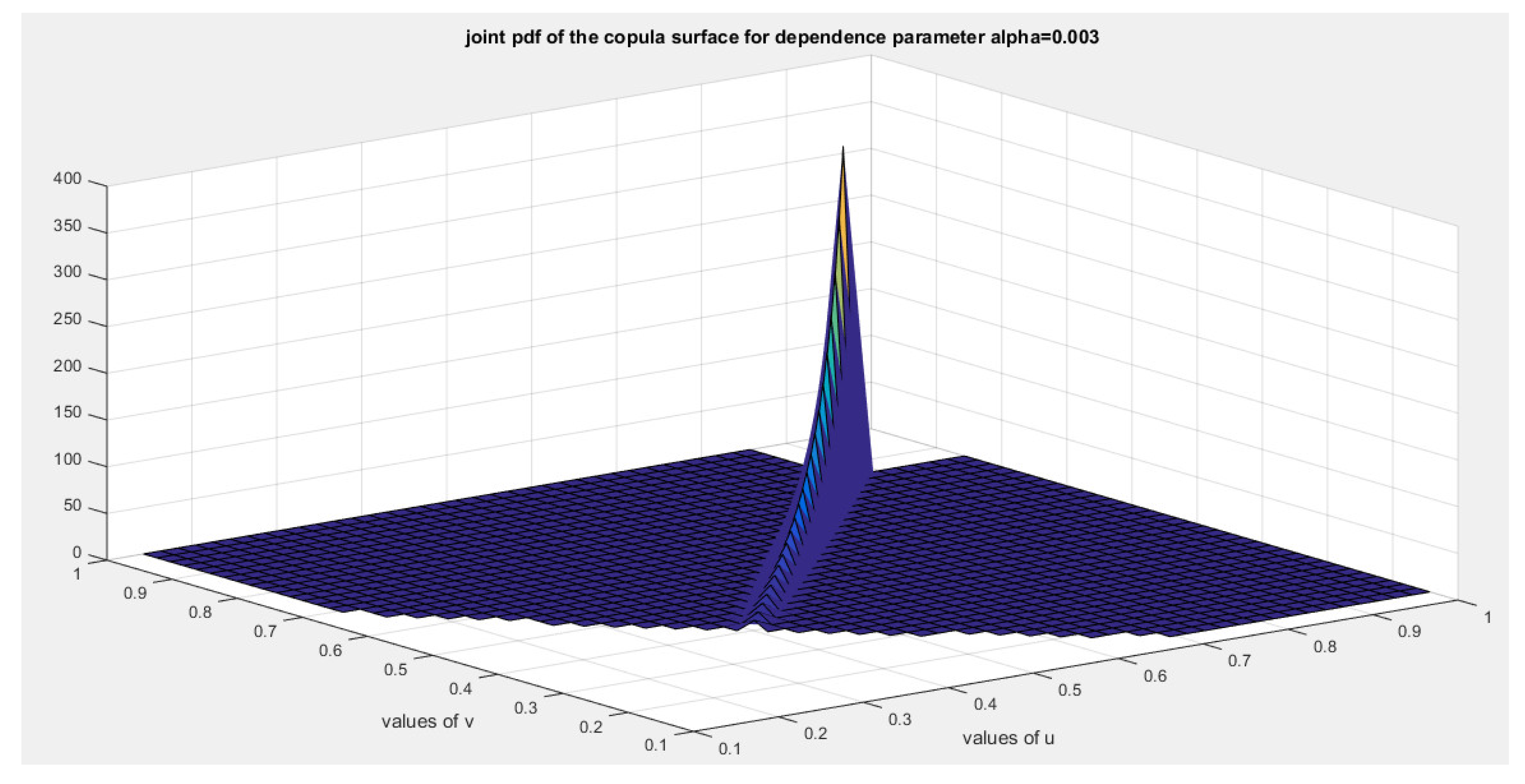
Figure 22.
shows the joint CDF copula at theta = 0.004.
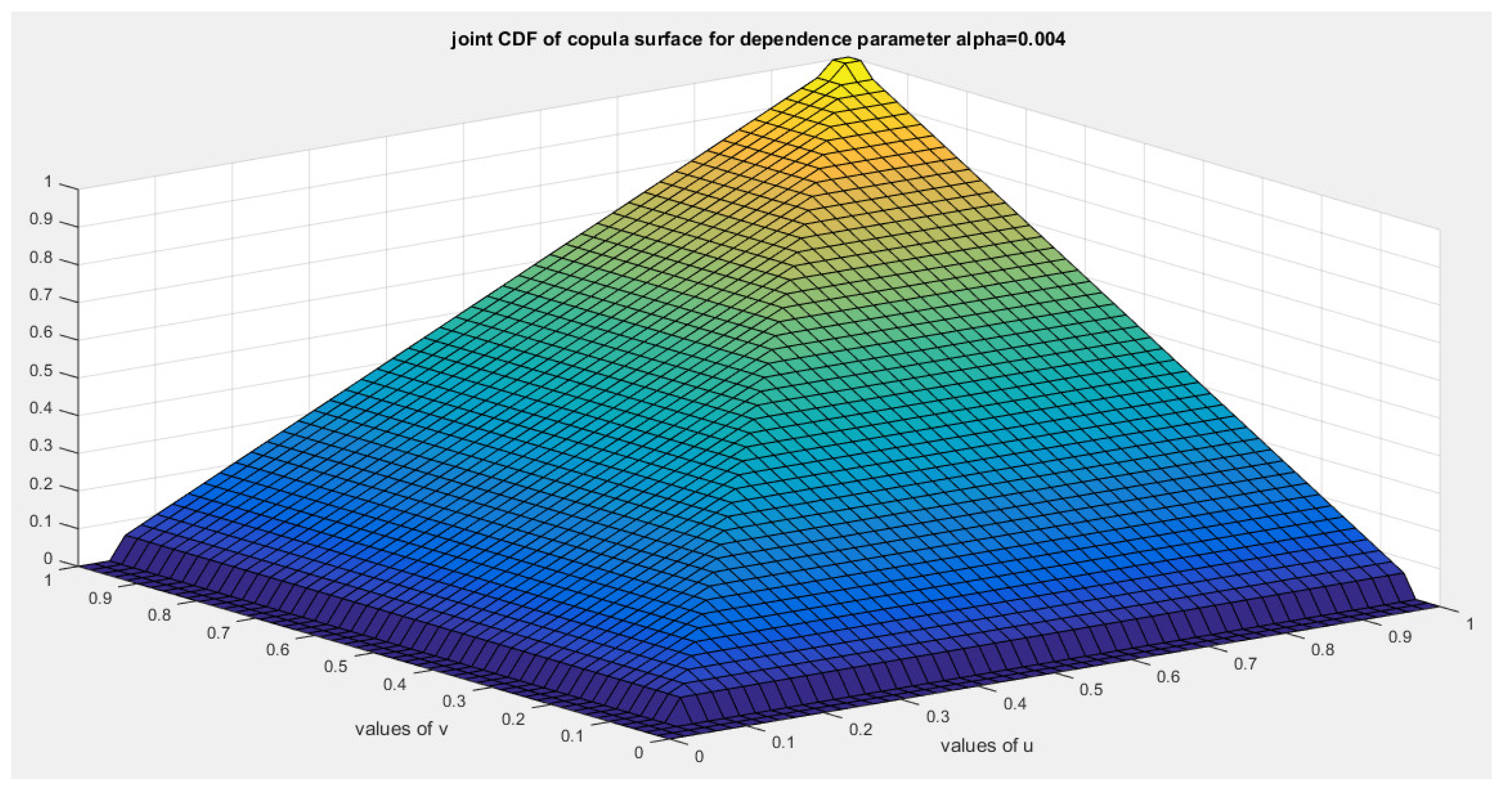
Figure 23.
shows the joint PDF copula at theta = 0.004.
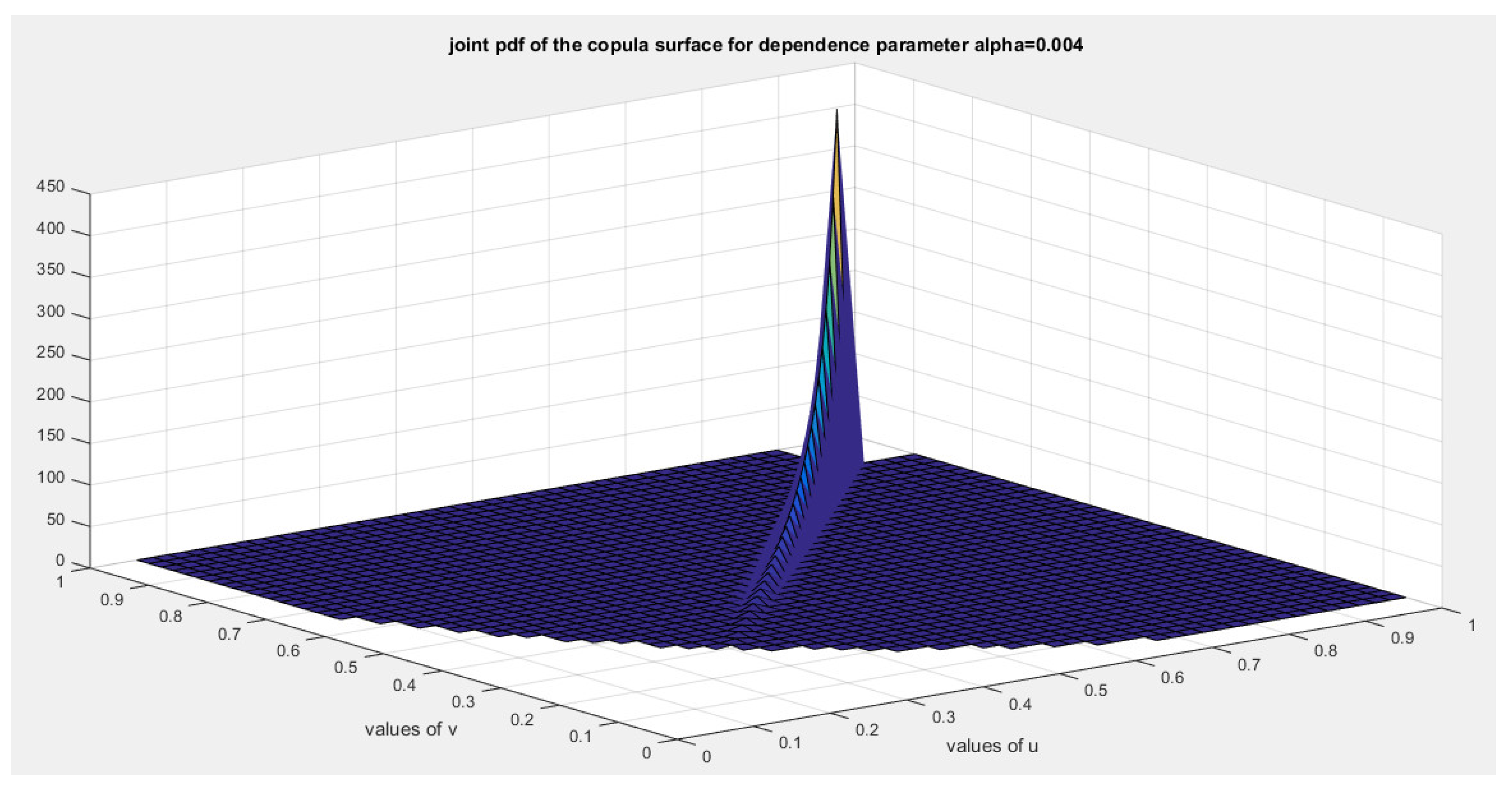
Figure 24.
shows the joint PDF copula at theta = 0.005.
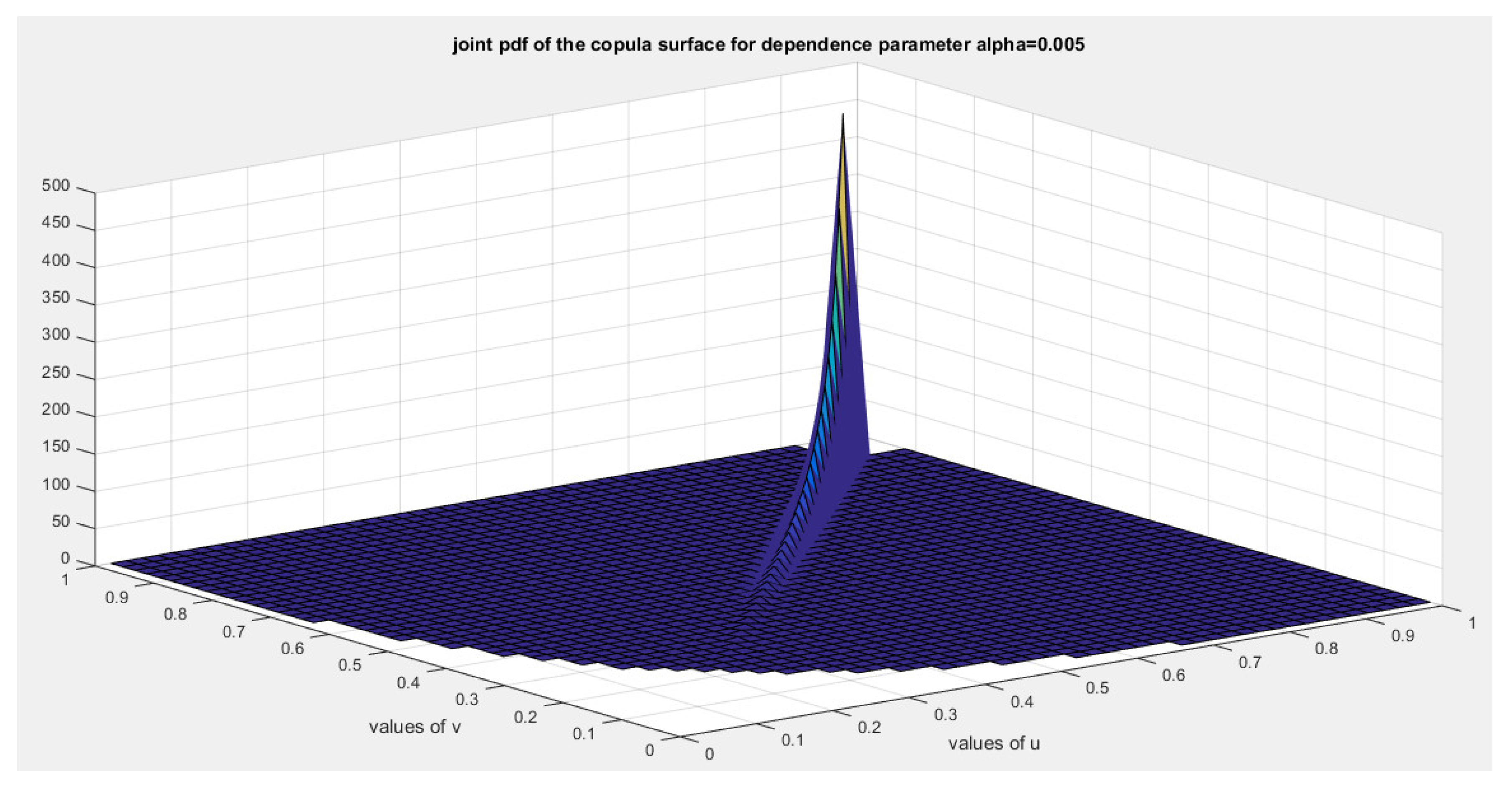
Figure 25.
shows the joint CDF copula at theta = 0.005.
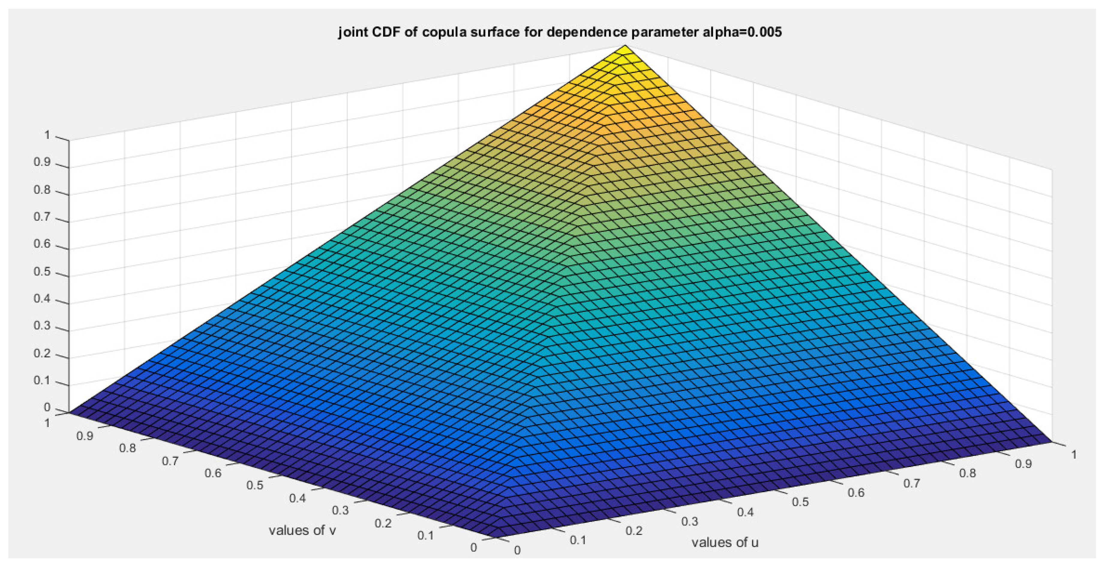
Figure 26.
shows the joint PDF copula at theta = 0.006.
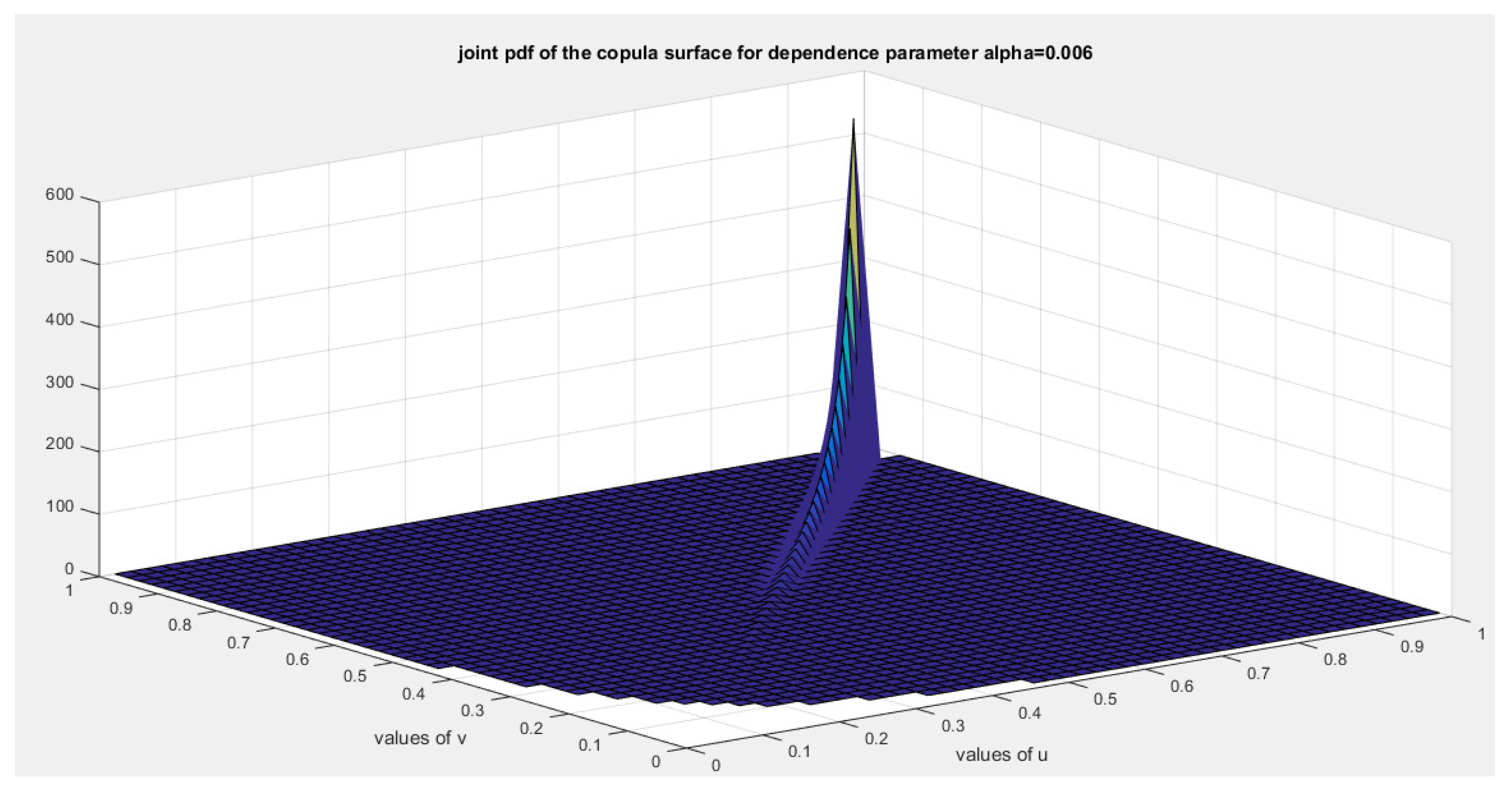
Figure 27.
shows the joint PDF copula at theta = 0.007.

Figure 28.
shows the joint PDF copula at theta = 0.008.
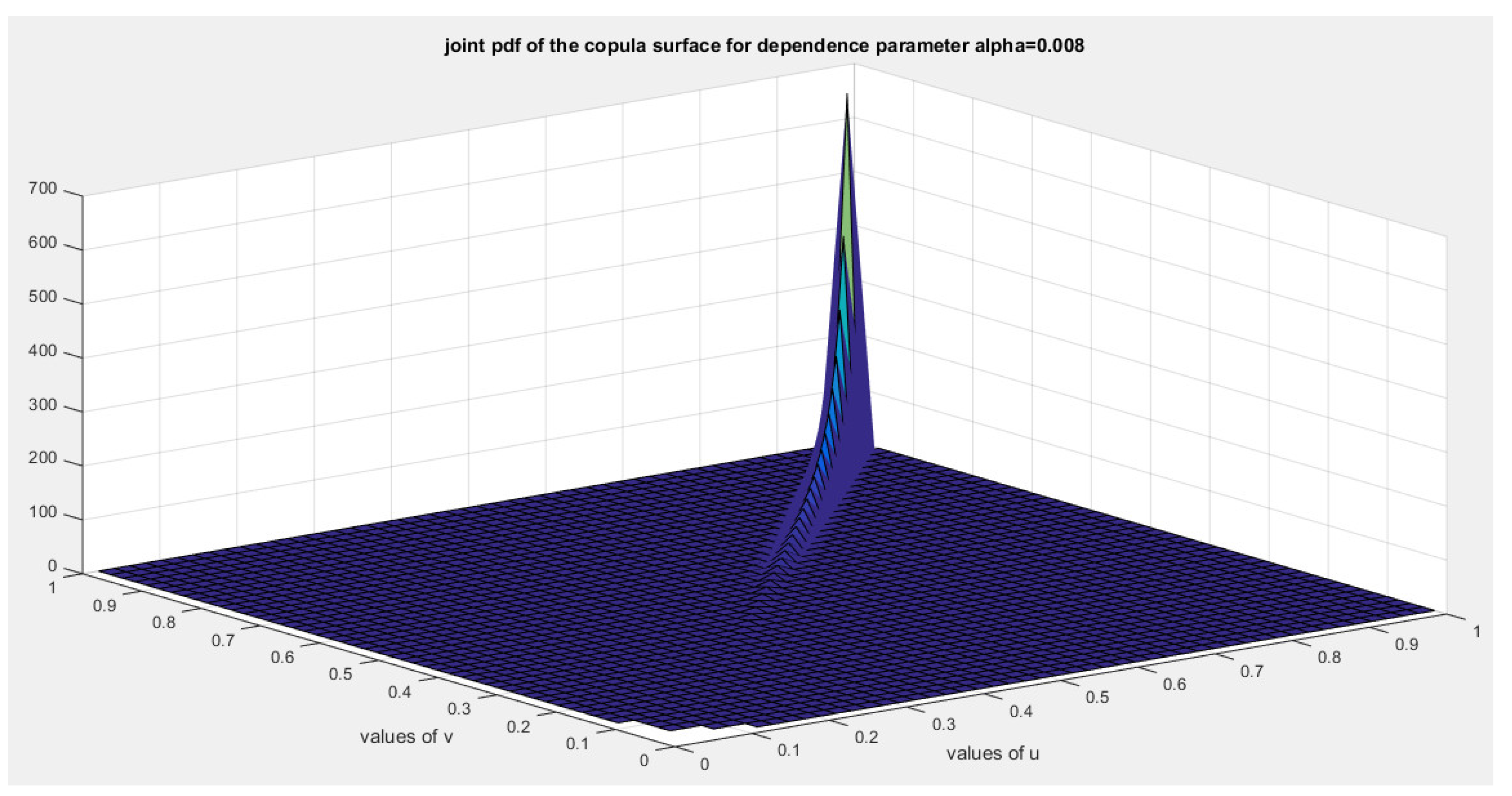
Figure 29.
shows the joint PDF copula at theta = 0.009.
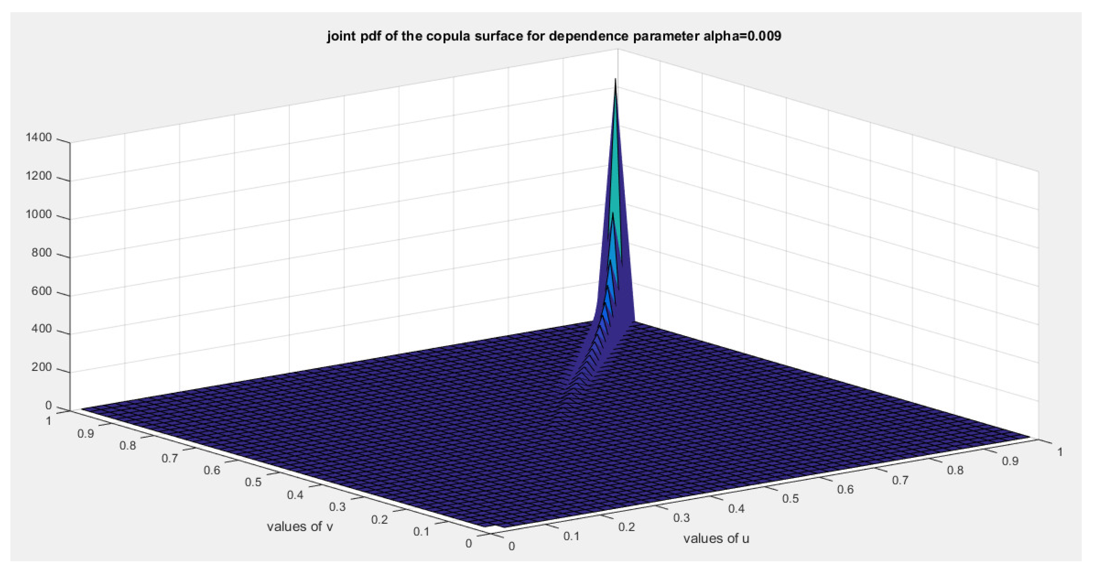
Figure 30.
shows the joint PDF copula at theta = 0.01.
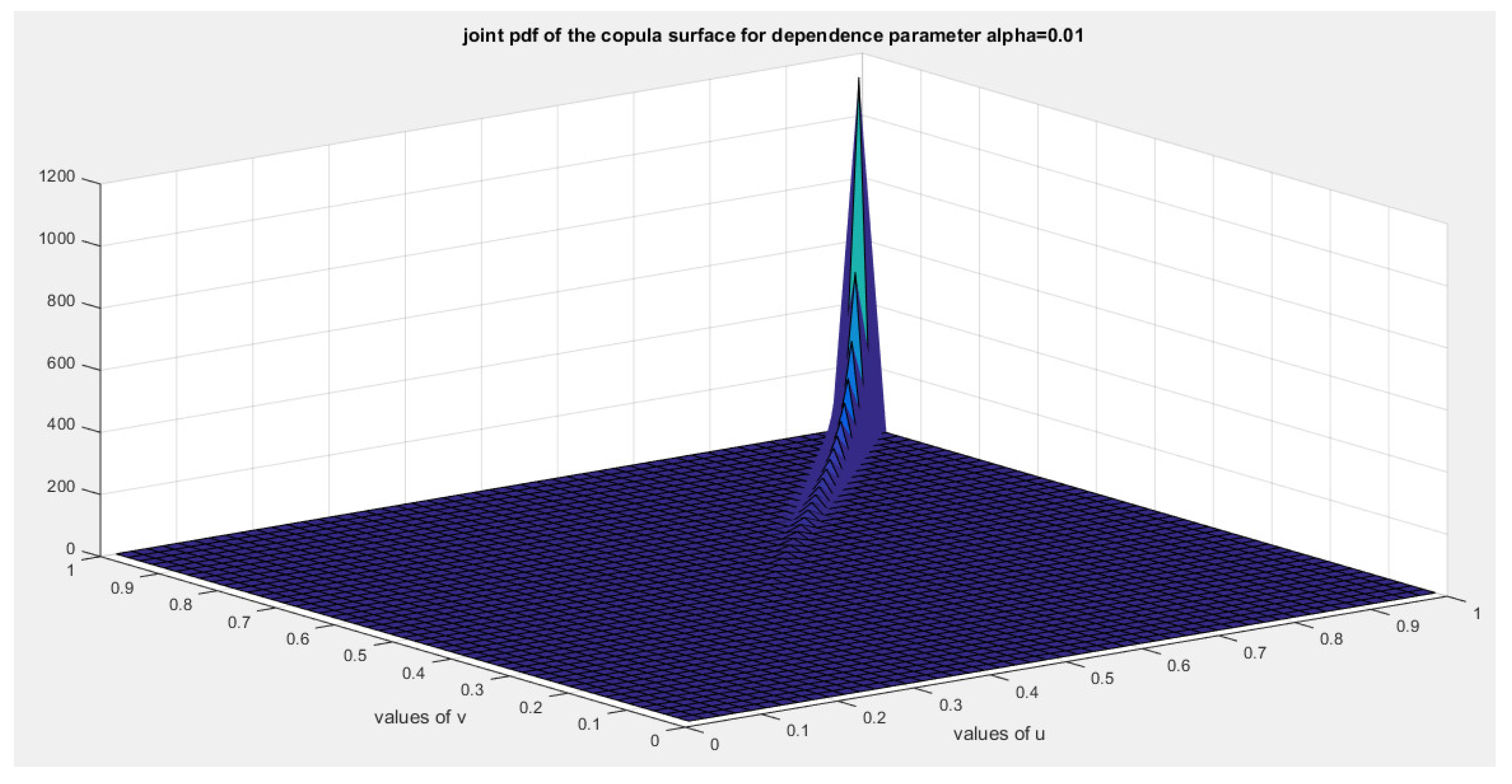
Figure 31.
tail dependency behavior of the Copula at dependency parameter 0.01.
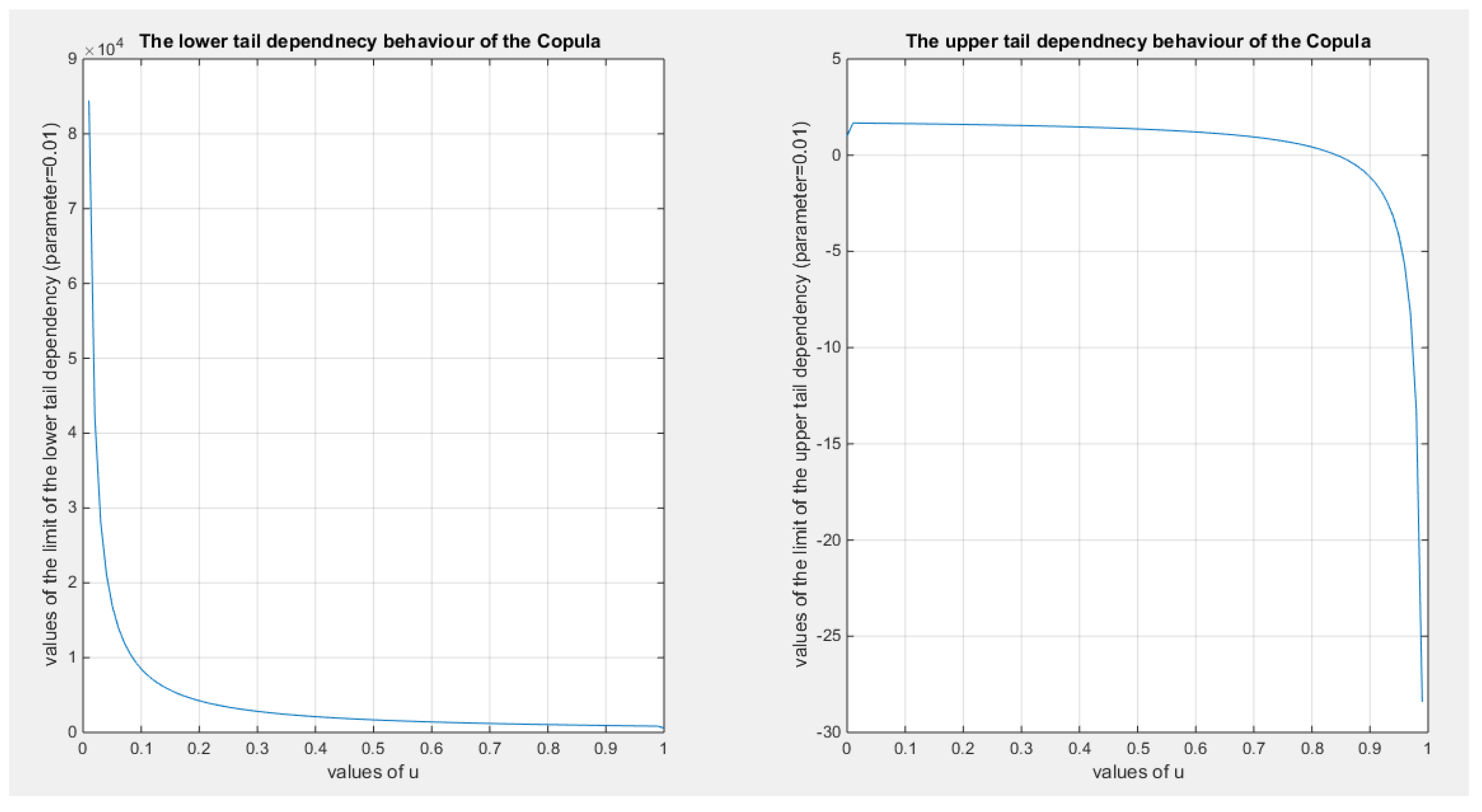
Figure 32.
tail dependency behavior of the Copula at dependency parameter 0.6.
Disclaimer/Publisher’s Note: The statements, opinions and data contained in all publications are solely those of the individual author(s) and contributor(s) and not of MDPI and/or the editor(s). MDPI and/or the editor(s) disclaim responsibility for any injury to people or property resulting from any ideas, methods, instructions or products referred to in the content. |
© 2025 by the authors. Licensee MDPI, Basel, Switzerland. This article is an open access article distributed under the terms and conditions of the Creative Commons Attribution (CC BY) license (http://creativecommons.org/licenses/by/4.0/).
Copyright: This open access article is published under a Creative Commons CC BY 4.0 license, which permit the free download, distribution, and reuse, provided that the author and preprint are cited in any reuse.


