
Submitted:
17 April 2025
Posted:
21 April 2025
You are already at the latest version
Abstract
Aortic stenosis is a valvular heart disease characterised by the narrowing of the valve opening area. Calcific and rheumatic aortic stenosis (AS) have distinctly different valve morphologies. The haemodynamic environment of generic calcific and rheumatic aortic valves of various severities is analysed through the use of 3D FSI modelling techniques. For moderate (AVA = 1-1.5 cm2), severe (AVA <1 cm2), and very severe (AVA ≪1 cm2) cases of calcific and rheumatic AS, larger TPGs with higher velocity magnitudes are estimated in the rheumatic cases compared to the calcific cases. The additional work required by the left ventricle to overcome the TPG caused by the moderate, severe, and very severe rheumatic valve lesions are 6.6 %, 42.5 %, and 58.3 % higher compared to the calcific valves of the same severity. The clinical approximation of the TPG is determined according to the simplified Bernoulli approximation and compared to the ground-truth TPG from the FSI results. The insensitivity of the clinical TPG approximation to the type and severity of stenosis is evident. Overall, the clinical approximation of the TPG either over or under predicts the TPG depending on the type and severity of the lesion, with smaller errors in the rheumatic cases compared to the calcific cases.
Keywords:
fuid structure interaction
; aortic valve pressure gradients
; rheumatic stenosis
; calcic stenosis
1. Introduction
Aortic stenosis (AS) or the narrowing of the aortic valve (AV) orifice, is the most common valvular lesion encountered in cardiology. Assessing the valve area and haemodynamic impact of the valve lesion is central to the management of this condition [1,2]. Calcific AS (CAS), commonly seen in older patients is the most prevalent cause of AS seen in high income countries [3]. In low- and middle income countries, including most countries in Sub-Saharan Africa, rheumatic AS (RAS), a late sequelae of rheumatic fever and rheumatic heart disease (RHD), is also a frequent case of AS. RHD is considered the most frequent cause of primary valvular heart disease (VHD), where up to 40 million people were affected in 2019 with an incidence of over 2 million per year [4]. Bicuspid aortic valve (BAV) is the most common congenital heart defect causing AS [5] however, the majority of AS cases seen in South Africa are caused by CAS or RAS.
The severity of AS is determined by the effect that the pathology has on the subsequent haemodynamic environment of the valve and is diagnosed by evaluating the mean transvalvular pressure gradient (TPG), the velocity profile of the blood flowing through the valve, the geometric and haemodynamic valve opening areas, and the function of the left ventricle. These geometrical and flow parameters are often determined through a combination of both invasive and non-invasive examination techniques. However, invasive cardiac catheterisation is only recommended in symptomatic cases with inconclusive non-invasive findings [1,2,5]. The classification ranges for these parameters are outlined in the guidelines published by the American College of Cardiology and the American Heart Association (ACC/AHA), and the European Society of Cardiology and European Association for Cardio-Thoracic Surgery (ESC/EACTS) [1,2].
When considering the two main causes of AS in South Africa, it is important to note that the pathology causing a reduction in AV area (AVA) results in differing valve morphologies, including the shape of the valve orifice, thereby impacting the TPG and the velocity profile of blood flowing through the valve. CAS is caused progressive fibrosis and calcification of the leaflets resulting in the semilunar leaflets becoming immobile and fixed in systole. The reduction in AVA due to CAS is characterised by the residual slit-like opening of the commisure between the leaflets. RHD leads to commissural fusion of the leaflets and the resulting reduced AVA found in RAS is characterised by a central triangular shaped orifice [6,7].
During systole, blood propelled out of the left ventricle through the systemic loop leads to a pressure differential across the aortic heart valve that causes the valve to open and close rhythmically. In the case of AS, the narrowing of the valve opening area leads to an increased resistance to the flow of blood which influences the mechanical work demand of the LV and results in an elevated TPG. As the relationship between the cardiac output and the pressure gradient across a stenosed valve is non-linear, it is important to determine the true TPG when diagnosing AS [8,9]. In a clinical setting, the anatomical and flow parameters of the defective valve are often analysed through transthoracic echocardiography (TTE) with 2D imaging and Doppler interrogation with the Doppler beam orientation parallel to the aortic valve blood jet. Through Doppler spectral analyses, the velocity profile is generated, and the TPGs are estimated according to a simplified Bernoulli correlation [1,2]. This correlation is empirically manipulated and derived from the Bernoulli equation for steady, incompressible and inviscid flow and relates the peak and mean jet velocity to the peak and mean TPG [10]. The uncertainty of the TPG estimation through the recommended Bernoulli correlation is well documented in recent studies [8,9,11,12,13,14,15,16,17,18] where efforts have been made to improve the accuracy through numerical and computational approaches. It is evident from the literature that the accuracy of the clinical TPG estimation in RHD and RAS cases is limited.
Studies where the TPG is estimated using steady-state computational fluid dynamics (CFD) approaches often consider the valve at peak systole conditions where either the peak or mean velocity conditions are used [8,17,18]. This results in peak TPG simulated measurements instead of the mean TPG diagnostic parameter or a mean TPG that is estimated at a peak AVA. As the AVA dynamically changes during systole, and there exists a non-linear relationship between the TPG and the velocity profile, it is possible that the mean TPG can not be accurately estimated at peak systole (and peak AVA) conditions. From a previous study by the authors, steady-state CFD simulations for various magnitudes of cardiac output (CO) indicated that there is a discrepancy between the haemodynamic environment of CAS and RAS of the same severity when considering the simulated TPG, the magnitude and location of the peak jet velocity (and therefore the location of the effective orifice area, EOA), and the corresponding clinical estimation of the TPG [8].
The simplifying assumptions associated with steady-state CFD analyses warranted further investigation using more complex modelling techniques. To overcome the limitation of steady-state CFD analyses of a compliant aortic valve, computational fluid-structure interaction (FSI) approaches are used. Through the use of FSI models, the dynamic behaviour of the deforming leaflets and the momentum and dampening of the blood flow is captured, allowing for a more accurate representation of the haemodynamic environment of the diseased aortic valves. In cardiovascular biomechanics, FSI has gained popularity due to the inclusion of both the structural and fluid domains when analysing the haemodynamics of the aortic heart valve [19,20]. More specifically, FSI models of the aortic heart valve include that of healthy native, synthetic or mechanical, and pathological valves mostly pertaining to calcific and bicuspid VHD [19,20,21,22,23,24,25,26,27,28,29]. To the best of the authors’ knowledge, there is no substantial literature regarding FSI modelling of RHD and RAS where the haemodynamic environments of the two AS pathologies are studied and compared to CAS simulated results.
The current work analyses the TPG and velocity profiles of the blood flow through generic calcific and rheumatic stenosed aortic valves by developing FSI models. For the same severity of AS, the effect of the different disease morphology on the aortic valve’s haemodynamic environment is evaluated. This includes the peak and mean TPGs, the peak and mean jet velocities, the location of the EOAs, and the lost work due to the pressure drop across the valves. Furthermore, the velocity profile at the EOA is used to estimate the corresponding peak and mean TPG according to the clinical Bernoulli equation and compare it to the corresponding simulated TPGs from the FSI models. The results from this numerical study provide a better understanding of the haemodynamic environment of the aortic valve in varying degrees of both calcific and rheumatic stenosed conditions and enable further discussion on the accuracy of the clinical TPG estimation in both disease types.
2. Materials and Methods
2.1. Description of Computational Domain
The computational domain assumes that the left ventricular outflow tract (LVOT), aortic valve, and aortic root are symmetrical about the axial axis. Therefore, of the entire three-leaflet aortic valve, the computational domain only considers one-sixth of the valve, i.e., half of one leaflet as illustrated in Figure 1 (a) and (b), where symmetry planes are used to create the full domain. The fluid domain includes the aortic root (upstream from the leaflet) modelled as rigid walls, a moving wall at the fluid-solid interface, a velocity profile at the inlet boundary condition (BC) shown in Figure 1 (c), and a constant pressure outlet BC [13,27,30]. In the current work, the compliance of the aortic root is disregarded in order to investigate the valve’s haemodynamic effect in isolation. The fluid domain shown in Figure 1 (a) does not represent the entire downstream and upstream regions. For a heartrate of 60/, the velocity profile over time for a single heartbeat of the cardiac cycle is shown in Figure 1 (c). These transient velocity profiles are generated for moderate, severe, and very severe cases of AS using the lumped parameter model (LPM) developed by Laubscher et al. (2022) [31]. The solid domain consists of a solid leaflet fixed within the LVOT.
2.2. Case Studies
The generic valve model [32,33] in each case study is based on the characteristics of the respective pathology. Similar generic pathological valve models were introduced in a previous study by the authors of the current work [8]. To represent the calcification of the leaflets in CAS cases, the leaflets are modelled as uniformly thickened structures where the thickness increases with an increase in severity [34]. The commissural fusion evident in RAS cases is mimicked by the fusion of a healthy native valve’s leaflet edges [7]. The moderately stenosed valve models are shown in Figure 2 where the thickening of the leaflets in the calcific case is indicated in (a), and the increased commissural fusion length in the rheumatic case is indicated in (b). It is important to note that the leaflet thickness in the RAS cases is considered to be that of a native valve (0.65), as the combined effect of calcification and commissural fusion is not considered in the current work. As a result, the characteristics of each pathology is evaluated in isolation, and its effect on the haemodynamic environment of the aortic valve is analysed.
The valve models are created during the FSI simulations according to the AVA measured at peak systole (i.e., peak BC and EOA velocity) for each severity which ranges between [range-units=single,range-phrase=-]11.5 for moderate AS, and < 1for severe and very severe AS [1,2]. The geometric valve opening area ratio (AR) is determined by the ratio of the AVA to the area of the LVOT at the base of the valve. Therefore, the AR at peak systole is governed by the severity of the disease, and is used to determine the thickness of the leaflets in the CAS cases and the fusion lengths in the RAS cases. The geometric parameters, AVA’s and AR’s at peak systole for each valve model are summarised in Table 1. The resultant moderate, severe, and very severe calcific and rheumatic valve models at peak systole conditions are discussed in Section 3. These valve models are included in the FSI simulations as deforming solid structures.
2.3. Modelling Theory
An FSI simulation is governed by the principle that the fluid and solid continua deform with the same kinematics and experience the same traction at the fluid-structure interface[35]. At the fluid-structure interface, fluid traction is transferred from the fluid domain to the solid domain resulting in deformation of the solid domain. Deformation of the solid domain in the form of displacement is consecutively transferred to the fluid domain, resulting in a two-way coupled FSI simulation. The FSI algorithm follows a partitioned approach where the fluid and structural equations are solved separately. The fully coupled fluid and structural solvers require a concurrent solution strategy and are formulated implicitly in time. The time dependent fluid domain () is solved within the fluid solver () and the time dependent structural domain () is solved within the structural solver (). To enable a two-way coupled FSI model of the blood flowing through and deforming the aortic valve, contact interfaces () between the structural and fluid surfaces at the valve are created [20,30].
In essence, the flow equations are solved for a given displacement (u) of the contact interface as a Dirichlet BC. The structural equations are solved for a given traction (T) at the contact interface as a Neumann BC. Therefore, at , the respective domains are solved according to Equation 1.
2.3.1. Fluid Flow Conservation Equations
Blood as the working fluid is considered incompressible and assumed to exhibit Newtonian behaviour at the geometric scale modelled in the present work [12,13,23,24,26,28,36]. The finite volume fluid flow solver () is based on the incompressible Navier-Stokes equations for Newtonian fluids [35,37]. The velocity and pressure fields are determined by the conservation of mass and momentum equations shown in Equation 2 for position vector . Note the momentum equations below are the Reynolds-averaged Navier-Stokes formulation.
In Equation 2, is the velocity vector in the , and directions respective, is the fluid density, is the fluid static pressure, and is the body force vector per unit fluid volume. The viscous stress tensor is given in Equation 3 where is the viscosity of the fluid.
The Reynolds stresses arising due to turbulent velocity fluctuations in the momentum equation (2 (b)) are closed using a turbulence model and the Boussinesq approximation shown in Equation 4 where the turbulent viscosity is denoted and the turbulent kinetic energy . The specifics of the turbulence model used in the present work will be discussed later.
2.3.2. Structure Mechanics Conservation Equations
The structural solver () uses the finite element method to solve the conservation of mass and momentum equations of the solid continuum and the constitutive equation of the material model [35,38]. For the position of a material point in the solid continuum in the undeformed configuration and in the deformed configuration , the deformation of displacement vector is given by Equation 5.
As a measure of the deformation change between points in the continuum, the deformation gradient tensor is defined and its determinant . The motion of a solid body is governed by Cauchy’s equilibrium where the displacement () of a solid body for is expressed according to the Lagrangian form of the law of conservation of momentum in Equation 6.
For the second material derivative in Equation 6, is the density of the solid, is the solid displacement vector in the , and direction, is the Cauchy stress tensor, and is the body force vector on the solid per unit volume. In the deformed configuration, is a measure of the traction acting on the surfaces of the solid body, and the Piola-Kirchhoff stress tensor () a measure of the traction acting on the surfaces of the solid body in the undeformed configuration. These tensors are related according to Equation 7.
The Cauchy stress tensor is related to the strain tensor according to the constitutive relations of the material model. For a hyperelastic material model, the general strain-stress relationship is given by Equation 8 where is the strain energy density function of the material described by the material model.
To ensure kinematic equilibrium between the fluid and solid domains with no-slip conditions at , the velocity vector of the fluid has to be equal to the velocity vector of the solid in Equation 9 [20].
Similarly, the traction of the fluid and the solid at is in equilibrium according to Equation 10. Here, the fluid stress tensor , and and are the respective unit normal vectors of and .
2.4. Model Development
The fluid solver () and structural solver () are coupled in a partitioned approach in Siemens STAR CCM+ (2402 build 19.02.009, Siemens Digital Industries Software, Plano, TX, USA [35]). The Arbitrary Lagrangian-Eulerian (ALE) technique is used to account for the solid displacement of in the fluid domain, where the fluid mesh is deformed and re-meshed to conform to the solid domain [28,30,35]. A first-order unsteady FSI model with a constant time step solves for a heartrate of 60/ and cardiac cycle of 1.0. The time step size depends on the case and ranges between [range-units=single,range-phrase=-]0.080.2 as a smaller time step is required to solve the FSI models with larger deformation gradients. A dynamic stabilisation method that adds force correction that is proportional to the displaced fluid per unit area as a pre-condition to the FSI interface is enabled to improve stability and ensure convergence at each iteration. The structutal solver is converged for absolute residuals of force and displacement below 1E-5. The fluid solver is converged for absolute residuals of continuity, momentum, and turbulence below 1E-6. The respective domains and their associated boundaries are discussed in Section 2.4.1 and Section 2.4.2 and are shown in Figure 3.
2.4.1. Fluid Domain
Blood is modelled as an incompressible Newtonian fluid with a density and dynamic viscosity of 995/ and 0.0035, respectively [8,31,36,39,40]. The fluid solver uses a SIMPLE implicit scheme with a realizable two-layer k- turbulence model and blended wall functions. As shown in Figure 3 (a), the fluid domain has rigid walls with no-slip conditions, two symmetry plane BC’s (A and B), a velocity inlet BC at the LVOT (shown in Figure 1 (c)), a constant pressure outlet BC of 0, and a no-slip displacement contact interface at . For the purpose of meshing and re-meshing efficiency, the fluid domain is divided into three regions; namely Fluid Core, Downstream and Upstream.
The Fluid Core region shown in Figure 3 (a) is discretised with polyhedral cells according to a mesh base size and target face size equal to the thickness of the leaflet. The polyhedral mesh is governed by a minimum cell surface size ranging between [range-units=single,range-phrase=-]1025 relative to the base size (depending on the case) and has a volume growth rate of 1.1. A two-layer prismatic cell layer with a thickness of 32 relative to the base size is generated at and the fluid walls. To conform the fluid vertices to the displaced solid structure, a new fluid mesh with a minimum face quality of 0.2 is generated in the Fluid Core region when the volume of a cell changes with [range-units=single,range-phrase=-]2540 (depending on the case) between time steps.
The Downstream and Upstream regions are generated from the respective downstream and upstream surfaces of Fluid Core region as 200 surface extrusions with the same fluid properties. As a result, boundary-type interfaces indicated in Figure 3 (a) between the respective fluid-fluid regions are generated. The extended regions are discretised with 160 layers of hexahedral cells where the cell sizes conform to the cell size of the neighbouring cells at the boundary interfaces (while the thickness of the cells remains constant). Therefore, the velocity inlet BC is applied at the downstream surface of the Downstream region (i.e., the LVOT), and the pressure outlet BC is applied at the upstream surface of the Upstream region. Each FSI model has a total fluid mesh size ranging between [range-units=single,range-phrase=-]135 000220 000cells, with 90 of the cells with a cell quality > 0.3 and a skewness angle < 40∘.
2.4.2. Solid Domain
The valve models described in Section 2.2 are included in the solid domain as shown in Figure 3 (b). The solid domain is modelled as a hyperelastic, isotropic, and homogeneous material with a density of 1000/. A Neo-Hookean material model in Equation 11 is used with a bulk modulus () of 53 and a C10 parameter of 0.1666[8,25,26] where is the first invariant of the deviatoric right Cauchy-Green deformation tensor, and J is the determinant of the deformation gradient tensor from Section 2.3.2.
Depending on the thickness of the leaflet, the solid domain is discretised with [range-units=single,range-phrase=-]9 50022 000cells quadrilateral elements with a minimum cell quality of 0.6 and a maximum skewness angle < 7∘. The leaflet has a fixed constraint at the base where it is attached to the LVOT as shown in Figure 3 (b), and a solid displacement contact interface at the surfaces. To ensure the leaflet deforms within the periodic symmetry boundaries of the computational domain, a displacement constraint in the direction perpendicular to symmetry plane A is applied at the side edge of the leaflet. To ensure the leaflet does not penetrate the imagined opposing leaflet, a contact plane at symmetry plane B with a gap offset of 0.2 to the inner surface of the leaflet is created as shown in Figure 3 (b). This prescribed clearance between the solid domain and the symmetry plane of the fluid domain is important to prevent the leaflet from deforming the fluid cells to zero volume.
2.4.3. Post Processing of Simulation Results
The simulated FSI results are analysed in MATLAB R2024a [41] to extract important haemodynamic values such as pressure gradients, stroke volume and lost work. The equations and parameters used to extract these and other important values will be discussed below.
The pressure gradient in s calculated at each time step as the difference between the mass flow averaged total pressure at the inlet and at the outlet of the fluid domain. All peak and mean TPG measurements in this text are converted to units of y dividing the pressure in y 133.33/. The velocity profiles in t the LVOT (i.e., the inlet BC due to fluid incompressibility) and at the EOA are evaluated. The peak and mean velocity conditions are determined from the velocity profiles as the maximum and the integral with respect to time, respectively. The EOA represents the area within a 4 radius from the centre of the domain where the velocity reaches its maximum. This prescribed radius represents the approximate diameter of an echo-Doppler ultrasound probe aligned parallel to the velocity jet [42].
The peak TPG from the FSI data is denoted and represents the maximum TPG calculated over the systolic period (). The mean TPG from the FSI results, denoted , is calculated as the time integral of the TPG over the systolic period in Equation 12.
The peak velocity at the EOA () is determined as the maximum velocity in the domain at timestamp . The TPG at timestamp is denoted . The mean velocity is calculated as the velocity time integral () of the jet velocity over the systolic period (time from valve opening to closing) according to Equation 13.
The timestamp associated with is denoted and is used to determine the TPG at timestamp denoted . The clinical TPG approximation is determined according to the simplified Bernoulli equation in Equation 14 where is the clinical TPG in nd V is the jet velocity in easured at the EOA.
The peak and mean TPGs, according to the clinical estimations, are therefore a function of the peak and mean velocities at the EOA and are denoted and , respectively in Equation 15.
The mass flow rate in n the domain is measured at each time step and is converted to volume flow rate (Q) in nd cardiac output () in The mean flow rate () in ver the systolic period is calculated as the time integral of Q over in Equation 16.
To quantify the impeding effect of the valve on the flow of blood, the lost work due to the pressure drop across the valve is calculated according to Equation 17 as the time integral of power (the product of TPG and Q) in ver the systolic period.
For a heartrate of 60/, the blood volume pumped out of the LV at each beat is called the stroke volume (SV) measured in The SV of a cardiac cycle is calculated from the time integral of Q over one heartbeat (T = 1.0) according to Equation 18.
3. Results and Discussion
The FSI models developed for moderate, severe, and very severe cases of CAS and RAS using the methods described in Section 2 is presented in this section. A grid convergence study is included in Section 3.1 followed by Section 3.2 that describes the necessary interpretation of the simulated FSI results presented in Section 3.3 and Section 3.4. For the same degree of stenosis, the CAS and RAS results are compared in Section 3.5. In this section, subscripts , , and refers to moderate, severe, and very severe CAS cases respectively. Similarly, , , and refers to moderate, severe, and very severe RAS cases respectively.
3.1. Mesh Convergence
A grid convergence study is performed on the initial fluid mesh of each FSI model to determine the optimal mesh size where the accuracy of the solution becomes independent of the computational grid [43]. The peak velocity and mean TPG at the EOA are used as the convergence criteria where a grid convergence index (GCI) in each case is calculated for a safety factor of 1.5 and a grid refinement ratio between 1.2 and 1.8. The mesh convergence results are summarised in Table 2. A maximum GCI of 1.85 for the peak velocity and 1.18 for the mean TPG is calculated in the moderate calcific case. As these GCI magnitudes are smaller than the recommended 4, the fluid meshes used in the FSI simulations are therefore considered converged and the solution sufficiently independent of the computational grids for the the current study.
3.2. Data Interpretation
The following data interpretation methodology applies to all case studies presented below:
- The systolic period () is calculated from the inlet velocity BC as the time when the velocity profile is positive. For the moderate, severe, and very severe CAS and RAS cases, the systolic periods are 0.2403, 0.2413 and 0.2554, respectively.
- With the exception of SV, all other data only pertains to the systolic period of the cardiac cycle. For the moderate, severe, and very severe CAS and RAS cases, the SV is 71.1/, 72.3/ and 68.1/, respectively.
- As the valve opens, the AR rapidly increases and fluctuates before it settles, whereafter it increases and decreases proportionally to the BC velocity profile. The valve is considered open after the AR has settled.
- Peak haemodynamic conditions are determined after the valve is considered open.
- The EOA velocity in the domain increases as the valve opens and reaches a maximum (). The time of peak EOA velocity () describes the phrase peak systole.
3.3. Calcific Aortic Stenosis
In Figure 4, the valve opening area ratio’s (left), EOA velocity (middle), and pressure gradient (right) results for the moderate ( Figure 4), severe ( Figure 4), and very severe ( Figure 4) CAS cases are shown. By analysing the AR profiles over the systolic period, in all cases, the AR increases rapidly during the opening phase of the valve, where it stabilises and is considered open at = 0.027, = 0.026, and = 0.015, respectively. The moderate CAS valve in Figure 4 has the longest opening phase with longer durations of AR oscillations compared to the more severe cases. This can be ascribed to the reduced stiffness of the valve body at lower levels of severity. From the EOA velocity profiles, the models reach peak systole at = 0.052, = 0.073, and = 0.12 respectively. The corresponding AR at peak systole is 0.330, 0.219, and 0.134, respectively, with peak velocities of = 3.69/, = 4.39/, and = 5.46/. The TPG recorded peak systole is = 40.5, = 60.23, and = 90.50 respectively. The AR and velocity profiles exhibit similar trends where the profile gradients decrease as the severity of CAS increases. This can be attributed to the reduced motion of the more severe leaflets, which enables the valve to reach peak systole later and remain at peak systole for longer periods before the valve starts to close.
From the pressure gradient profiles, the true peak TPG in each case is recorded at = 0.03, = 0.029, and = 0.015. This indicates that the maximum pressure gradient in the domain is reached before the model reaches peak systole with pressure gradients of = 83.30, = 97.50, and = 114.75. Therefore, as the true peak TPG is not recorded at peak systole, the respective TPG estimations at peak systole are 42.8, 37.3, and 24.3 lower than the true peak TPG for the moderate, severe, and very severe CAS cases, respectively. The findings indicate that relying solely on to estimate the TPG using methods such as echo-Doppler for the present modelled examples will result in an underestimation of the TPG.
The mean velocity and TPG in the moderate, severe, and very severe CAS cases are = 2.84/ and = 10.2, = 3.63/ and = 34.85, and = 4.77/ and = 77.59, respectively This indicates a relative percentage increase in VTI values of 27.82 between moderate and severe cases and 31.4 between severe and very severe cases. Similarly, the mean gradient shows percentage increases of 241 from moderate to severe cases and 122 from severe to very severe cases.
From the pressure gradient profiles in Figure 4, the TPG profiles decrease proportionally to the valve area as the valve starts to close. As the moderate calcific valve opens and closes more rapidly compared to the more severe cases, the TPG profile is expected to have the steepest gradients with an almost linear decrease as the AR decreases. The severe and very severe CAS cases have similar TPG profile trends where the pressure gradient gradually decreases proportionally to the AR, where the TPG remains relatively constant during peak systole in the very severe case. As a result, the mean haemodynamic conditions are closer in magnitude to the peak haemodynamic conditions as the severity of CAS increases.
3.4. Rheumatic Aortic Stenosis
Similar to the CAS cases, the valve opening area ratios (left), EOA velocity (middle), and pressure gradient (right) results for the moderate, severe, and very severe RAS cases are shown in Figure 5. The AR profiles of the RAS cases exhibit similar trends to the CAS cases where the AR increases and fluctuates before it settles and is considered open at = 0.026, = 0.023, and = 0.021. However, from the AR profiles of the RAS cases, it can be seen that these valve models reach fully open states later and exhibit fewer oscillations of the AR compared to the CAS cases. The respective RAS cases reaches peak systole at = 0.043, = 0.076, and = 0.11. At peak systole, the moderate, severe, and very severe cases have corresponding AR’s of 0.335, 0.222, and 0.138, maximum EOA velocities of = 4.18/, = 5.73/, and = 7.54/, and pressure gradients of = 53, = 105, and = 200, respectively. Therefore, as the severity of RAS increases, the geometric opening area decreases, resulting in a decreased AR. The AR and velocity profiles are observed to require more time to reach fully open and peak systole states, and the valves remain at peak systole for longer periods before the valve start to close.
The true peak TPG is, again, measured before peak systole is reached at = 0.03, = 0.029, and = 0.047. The true peak TPG for each of the cases are = 90, = 135, and = 207. The respective TPG estimations at peak systole are therefore of 37, 30, and 7 lower than the true peak TPG in the moderate, severe, and very severe RAS cases, respectively. The pressure gradient profile increases and decreases rapidly in the moderate case and more gradually in the severe case. In the very severe RAS case the TPG remains relatively constant at 200 before it reduces rapidly at the end of the systolic period.
The mean haemodynamic conditions for the respective RAS cases are calculated as = 2.87/ and = 37.28, = 4.61/ and = 82.76, and = 6.79/ and = 173.57. As observed in the CAS cases, the difference between the peak and mean velocity and pressure gradient magnitudes decreases with an increase in severity. These results indicate a relative percentage increase in VTI values of 60.6 between moderate and severe cases and 47.3 between severe and very severe cases. Similarly, the mean gradient shows percentage increases of 122 from moderate to severe cases and 109 from severe to very severe cases. This demonstrates that as severity increases, RAS cases exhibit greater relative increases in VTI changes between severity levels and smaller relative increases in pressure gradients compared to CAS cases.
3.5. General Comparison Between CAS and RAS
The effect of each disease morphology on the flow of blood through the valve is determined by comparing the results discussed in Section 3.3 and Section 3.4. The generic valve models for the moderate, severe, and very severe calcific and rheumatic cases at peak flow conditions are shown in Figure 4 and Figure 5 and the AR’s and AVA’s summarised in Table 1. From Figure 4 and Figure 5, it can be seen that for the same severity and similar AVAs and ARs, the two pathologies produce distinctly different opening morphologies where the calcific valve area has a more star-like shape, and the rheumatic valves a more circular and triangular shape. Consequently, calcific valves have smaller hydraulic diameters than their equivalent RAS valves, resulting in lower Reynolds numbers and reduced frictional and secondary loss effects. This is evident in the previously mentioned results, where RAS valves exhibit substantially higher TPG values for the same ARs. Furthermore, it is evident that the rheumatic valve models experience more severe bulging due to the decreased stiffness of the leaflets, and reach fully open valve states faster and with smaller AR fluctuations during the opening phase compared to the calcific models.
The impeding effect of the diseased valves on the flow of blood is quantified by the mean flow rate (Equation 16) and the lost work (Equation 17) experienced by the blood flowing through the aortic valve. The mean flow rate indicates the CO of the left ventricle-aortic valve combination, and the lost work indicates the additional work required by the ventricle to overcome the valvular pressure drop. These values (mean flow rate and lost work ) are shown for the different morphologies and severities in Table 3. The peak and mean velocity magnitudes are used to determine the clinical TPG estimations according to Equation 15 and compared to the ground truth FSI results. These values are also shown in the table below.
For each severity of AS, the same velocity profile is used for both calcific and rheumatic cases. Therefore, the SV describing the volume of blood pumped out of the LV at each heartbeat remains the same for both pathologies with the same stenosis severity. The moderate, severe, and very severe cases have SV’s of 71.1/, 72.3/, and 68.1/, respectively. For the same SV, the mean flow rate in Table 3 is higher in the RAS cases compared to the CAS cases. The lost work in the RAS cases are 6.6, 42.5, and 58.3 higher compared to the CAS cases for moderate, severe, and very severe cases, respectively, which alludes to the higher resistance the RAS valves offer to the flow of blood compared to the CAS valves. As a result, the LV must work harder in the presence of rheumatic stenosed valves to overcome the pressure drop caused by the pathology compared to the calcific stenosed valves of the same severity. Furthermore, the mean flow rate decreases with an increase in severity, which is proportional to the decrease in SV, and the lost work increases with an increase in severity due to the higher pressure gradients experienced by the more severe valves. The mean flow rate and lost work is, therefore, a function of the severity of stenosis (i.e., SV) and the type of stenosis described by the morphology of the valve.
The peak TPG recorded from the FSI data is compared to the TPG at the time of peak velocity () to determine the relative timing of the EOA velocity and pressure profiles as discussed in Section 3.3 and Section 3.4. The peak and mean velocity and TPG measurements increase proportionally to the degree of stenosis in both cases. The moderate, severe, and very severe peak EOA velocities in the RAS models are 0.49/, 1.34/, and 2.08/ higher than the corresponding CAS models. Similarly, the mean velocity in the RAS cases are 0.03/, 0.98/, and 2.02/ higher than the CAS cases. Due to the high-velocity profiles evident in the rheumatic cases, the peak and mean TPGs are expected to be higher than the calcific cases. The peak TPG () in the rheumatic cases are 7, 28, and 45 higher than in the corresponding CAS case. The mean TPG in the RAS cases are 73, 58, and 55 higher than the respective CAS cases.
As the clinical estimation of the pressure gradient is a function of velocity only (Equation 15), the clinical peak TPG () and clinical mean TPG () estimations are compared to the respective peak and mean FSI estimations summarised in Table 3. In the calcific case, with respect to the true peak TPG, the peak clinical TPG underestimates the pressure gradient by 28.7 in moderate and 20.3 in severe and overestimates the pressure gradient by 4.3 in the very severe case. Conversely, the mean clinical estimations are consistently overestimated by 22.2, 18, and 13 in moderate, severe, and very severe CAS cases, respectively. From these errors, it is clear that the clinical pressure estimation either under or overestimates the pressure gradient depending on the severity of the calcifications. In the rheumatic case, the peak clinical TPG estimation is 20 and 3.8 lower than the FSI results for the moderate and severe cases and 20.3 higher in the very severe case. The mean clinical TPG estimation is 4.3 lower in the moderate case and 2.2 and 10.7 higher in the severe and very severe cases. As is seen in the calcific models, the clinical estimations in the RAS cases are again inconsistent as they either underestimate or overestimate the pressure gradient depending on the severity of the disease. However, the clinical TPG estimation errors are higher in the CAS cases compared to the RAS cases.
In Figure 6, Figure 7, and Figure 8, the velocity contours (left) and TPG-Q relationships (right) are shown for each severity of AS along a plane orientated to cut through two of the valve leaflets. The velocity contour at peak systole is used to determine the velocity jet’s shape and the EOA’s location in the jet. The relationship between the pressure gradient and the flow rate is evaluated by presenting the TPG at each volume flow rate where the colour and the opacity of the data points are a function of the AR. The TPG-Q relationships in these figures are generated by analysing the system curve for each data point as a function of AR. Therefore, each data point represents the instantaneous TPG and Q at a specific AR as the valve opens and closes and allows for the analysis of the combined resultant system curve (not to be confused with a typical fluid system quadratic system curve) for each case during the time when the flow is nearly or fully established.
As mentioned in Section 2.2, the stenosis present in the rheumatic valve models is only a function of the commissural fusion length, not the leaflet thickness. The stiffness of the leaflets in the RAS cases is therefore not influenced by the degree of stenosis to the same extent as in the CAS cases. It explains the excessive bulging of these valves and the elevated pressure gradients seen in Figure 5. Although the two pathologies are governed by the same severity when considering AR and SV, the increased jet velocity and pressure gradient profiles in the rheumatic cases can be attributed to the morphology of the valve area reduction. At peak systole, the morphology of the rheumatic valves closely resemble that of an orifice (although not perfectly circular), compared to a star-like valve morphology of the calcific valves. The contraction mechanism drives the velocity jets in both the CAS and RAS cases and, therefore, friction at the valve walls proximal to the AVA, and sudden expansion distal to the AVA. As a result of the different valve morphologies, the velocity jet in the RAS cases is more concentrated and less dispersed compared to the CAS cases, as seen in the velocity contour plots at peak systole illustrated in Figure 6, Figure 7, and Figure 8. The higher velocity jet core zones in the rheumatic valves result in larger magnitudes of shear stresses, higher energy dissipation, and, as a result, greater pressure gradients. From the velocity contour plots it is evident that as the severity of the stenosis increases, the EOA moves proximal to the valve in the CAS cases, and more distal in the RAS cases.
From the TPG-Q relationship in the moderately stenosed cases in Figure 6 and Figure 6, the calcific and rheumatic cases follow similar trends where the TPG increases with an increase in flow rate. At an AR of 0.33, the moderate CAS and RAS valves are fully open. For AR’s between 0.28 and 0.33 and volume flow rates between [range-units=single,range-phrase=-]300450/, the TPG increases at a rate of 0.14/ in MC case compared to 0.19/ in MR case. Therefore, the TPG in the moderate cases increases at a 26 higher rate in the rheumatic valve as it approaches fully open and peak systole states.
As with the moderate valves, the TPG-Q relationship in the severe cases in Figure 7 and Figure 7 also follow similar trends where the TPG in both disease types increases with an increase in flow rate. The severe models reach fully open states with an AR of approximately 0.22. For ARs between 0.17 and 0.22 and volume flow rates between [range-units=single,range-phrase=-]300450/, the TPG-Q gradient is 0.35/ in the SC case and 0.38/. Therefore, the TPG in the severe cases increases at an 8 higher rate in the rheumatic valve compared to the calcific valve when it approaches fully open and peak systole states.
The velocity jet in the very severe calcific model in Figure 8 (left) develops upstream with a longer, more dispersed jet compared to the very severe rheumatic case in Figure 8 (left). The TPG-Q relationship in the very severe cases in Figure 8 and Figure 8 (right) follow slightly different trends compared to the less severe cases. However, the TPG still increases as the volume flow rate increases. At least two trends with varying gradients can be identified for this severity. For flow rates below 150/, the VSR model in Figure 8 has an approximate linear TPG-Q gradient of 1.4/ and for volume flow rates between [range-units=single,range-phrase=-]200350/ with AR’s between 0.08 and 0.13, it has a gradient of 0.4/. Alternatively, the VSC model in Figure 8 has gradients of 2.7/ for flow rates between 100/ and 200/ and 0.58/ for volume flow rates between 200/ and 350/ and AR’s between 0.08 and 0.13. Therefore, the TPG increases at a rate that is 48 and 31 higher in the VSC case compared to the VSR case for volume flow rates of [range-units=single,range-phrase=-]100200/ and [range-units=single,range-phrase=-]200350/, respectively. It is however important to note the difference in TPG magnitude between the two cases where the TPG in the VSR model is approximately double the TPG in the VSC model.
4. Conclusions
The results show that the haemodynamic behaviour of stenosed aortic heart valves depends on the disease’s type and severity. Calcific and rheumatic aortic stenosis is modelled by considering the characteristics of the respective pathologies and, through the use of FSI modelling methodologies, the haemodynamic conditions in the aortic valve lesions are determined by analysing the velocity profiles, pressure gradients and lost work in the domain. The results show that, for all severities of stenosis, the rheumatic valves offer higher resistance to the flow of blood compared to the calcific valves for similar flow rates and areas. The velocity profiles in the rheumatic cases have higher magnitudes with more concentrated and less dispersed velocity jets than the calcific cases. Consequently, the pressure gradients are higher in the rheumatic cases than in the calcific cases. Velocity reaches a maximum at the vena contracta (i.e., EOA) located proximal to the valve in the CAS cases and distal to the valve in the RAS cases. The clinical estimation of the pressure gradient is considered to determine the impact that the type of stenosis has on the estimated TPG according to the simplified Bernoulli equation used in clinical practice. The results emphasise the insensitivity of the clinical estimation on valve morphology as it either under- or overestimates the TPG depending on the type and the severity of the valve lesion. Therefore, it can be concluded from this numerical study, considering the dynamics of the opening and closing of the aortic valve in isolation, that the morphology of the valve has a significant effect on the haemodynamic conditions of stenosed aortic valves and that the clinical estimation generally performs better in predicting the TPG in the RAS cases compared to the CAS cases.
Author Contributions
Model development, L.G.K. and R.L.; data analysis, L.G.K., R.L., J.v.d.M., M.P.V., and P.G.H.; original draft preparation, L.G.K.; review and editing, L.G.K., R.L., M.P.V., J.v.d.M., A.F.D., and P.G.H.; visualization, L.G.K., R.L., and J.v.d.M.; project administration, L.G.K., R.L., J.v.d.M., and P.G.H.; funding acquisition, L.G.K. and R.L.; All authors contributed to the critical review and revision of the manuscript.
Funding
This work is based on the research supported in part by the National Research Foundation of South Africa (reference number PMDS22071138485).
Acknowledgments
The authors would like to thank the support team at Siemens AG for their support and assistance.
Conflicts of Interest
The authors declare no conflicts of interest.
References
- Otto, C.M.; Nishimura, R.A.; Bonow, R.O.; Carabello, B.A.; Erwin, J.P.; Gentile, F.; Jneid, H.; Krieger, E.V.; Mack, M.; McLeod, C.; et al. 2020 ACC/AHA Guideline for the Management of Patients With Valvular Heart Disease: A Report of the American College of Cardiology/American Heart Association Joint Committee on Clinical Practice Guidelines. Journal of the American College of Cardiology 2021, 77, e25–197. [Google Scholar] [CrossRef] [PubMed]
- Vahanian, A.; Beyersdorf, F.; Praz, F.; Milojevic, M.; Baldus, S.; Bauersachs, J.; Capodanno, D.; Conradi, L.; Bonis, M.D.; Paulis, R.D.; et al. 2021 ESC/EACTS Guidelines for the management of valvular heart disease: Developed by the Task Force for the management of valvular heart disease of the European Society of Cardiology (ESC) and the European Association for Cardio-Thoracic Surgery (EACTS). European Heart Journal 2022, 43, 561–632. [Google Scholar] [CrossRef]
- Timmis, A.; Aboyans, V.; Vardas, P.; Townsend, N.; Torbica, A.; Kavousi, M.; Boriani, G.; Huculeci, R.; Kazakiewicz, D.; Scherr, D.; et al. European Society of Cardiology: the 2023 Atlas of Cardiovascular Disease Statistics. European Heart Journal 2024, 45, 4019–4062. [Google Scholar] [CrossRef]
- Coffey, S.; Roberts-Thomson, R.; Brown, A.; Carapetis, J.; Chen, M.; Enriquez-Sarano, M.; Zühlke, L.; Prendergast, B.D. Global epidemiology of valvular heart disease. Nature Reviews Cardiology 2021, 18, 853–864. [Google Scholar] [CrossRef]
- Yang, L.T.; Ye, Z.; Ullah, M.W.; Maleszewski, J.J.; Scott, C.G.; Padang, R.; Pislaru, S.V.; Nkomo, V.T.; Mankad, S.V.; Pellikka, P.A.; et al. Bicuspid aortic valve: long-term morbidity and mortality. European Heart Journal 2023, 44, 4549–4562. [Google Scholar] [CrossRef] [PubMed]
- Alizadeh, L.; Peters, F.; Vainrib, A.F.; Freedberg, R.S.; Saric, M. Rheumatic Heart Disease: A Rare Cause of Very Severe Valvular Aortic Stenosis. CASE 2024, 8, 320–324. [Google Scholar] [CrossRef]
- Afifi, A.; Hosny, H.; Yacoub, M. Rheumatic aortic valve disease-when and who to repair? Annals of Cardiothoracic Surgery 2019, 8, 383–389. [Google Scholar] [CrossRef] [PubMed]
- Grobler, L.; Laubscher, R.; van der Merwe, J.; Herbst, P.G. Evaluation of Aortic Valve Pressure Gradients for Increasing Severities of Rheumatic and Calcific Stenosis Using Empirical and Numerical Approaches. Mathematical and Computational Applications 2024, 29. [Google Scholar] [CrossRef]
- Franke, B.; Weese, J.; Waechter-Stehle, I.; Brüning, J.; Kuehne, T.; Goubergrits, L. Towards improving the accuracy of aortic transvalvular pressure gradients: rethinking Bernoulli. Medical & and Biological Engineering & Computing 2020, 58, 1667–1679. [Google Scholar] [CrossRef]
- Hatle, L.; Brubakk, A.; Tromsdal, A.; Angelsen, B. Noninvasive assessment of pressure drop in mitral stenosis by Doppler ultrasound. British Heart Journal 1978, 40, 131–140. [Google Scholar] [CrossRef]
- Pase, G.; Brinkhuis, E.; Vries, T.D.; Kosinka, J.; Willems, T.; Bertoglio, C. A parametric geometry model of the aortic valve for subject-specific blood flow simulations using a resistive approach. Biomechanics and Modeling in Mechanobiology 2023, 22, 987–1002. [Google Scholar] [CrossRef]
- Hellmeier, F.; Brüning, J.; Sündermann, S.; Jarmatz, L.; Schafstedde, M.; Goubergrits, L.; Kühne, T.; Nordmeyer, S. Hemodynamic Modeling of Biological Aortic Valve Replacement Using Preoperative Data Only. Frontiers in Cardiovascular Medicine 2021, 7, 593709. [Google Scholar] [CrossRef]
- Hoeijmakers, M.J.; Waechter-Stehle, I.; Weese, J.; de Vosse, F.N.V. Combining statistical shape modeling, CFD, and meta-modeling to approximate the patient-specific pressure-drop across the aortic valve in real-time. International Journal for Numerical Methods in Biomedical Engineering 2020, 36, e3387. [Google Scholar] [CrossRef] [PubMed]
- Harris, P.; Kuppurao, L. Quantitative Doppler echocardiography. BJA Education 2016, 16, 46–52. [Google Scholar] [CrossRef]
- Ha, H.; Lantz, J.; Ziegler, M.; Casas, B.; Karlsson, M.; Dyverfeldt, P.; Ebbers, T. Estimating the irreversible pressure drop across a stenosis by quantifying turbulence production using 4D Flow MRI. Scientific Reports 2017, 7. [Google Scholar] [CrossRef]
- Kazemi, A.; Padgett, D.A.; Callahan, S.; Stoddard, M.; Amini, A.A. Relative pressure estimation from 4D flow MRI using generalized Bernoulli equation in a phantom model of arterial stenosis. Magnetic Resonance Materials in Physics, Biology and Medicine 2022, 35, 733–748. [Google Scholar] [CrossRef] [PubMed]
- Liu, X.; Guo, G.; Wang, A.; Wang, Y.; Chen, S.; Zhao, P.; Yin, Z.; Liu, S.; Gao, Z.; Zhang, H.; et al. Quantification of functional hemodynamics in aortic valve disease using cardiac computed tomography angiography. Computers in Biology and Medicine 2024, 177, 108608. [Google Scholar] [CrossRef]
- Franke, B.; Brüning, J.; Yevtushenko, P.; Dreger, H.; Brand, A.; Juri, B.; Unbehaun, A.; Kempfert, J.; Sündermann, S.; Lembcke, A.; et al. Computed Tomography-Based Assessment of Transvalvular Pressure Gradient in Aortic Stenosis. Frontiers in Cardiovascular Medicine 2021, 8, 706628. [Google Scholar] [CrossRef]
- Kuchumov, A.G.; Makashova, A.; Vladimirov, S.; Borodin, V.; Dokuchaeva, A. Fluid–Structure Interaction Aortic Valve Surgery Simulation: A Review. Fluids 2023, 8. [Google Scholar] [CrossRef]
- De Hart, J.; Peters, G.W.M.; Schreurs, P.J.G.; Baaijens, F.P.T. A three-dimensional computational analysis of fluid-structure interaction in the aortic valve. Journal of Biomechanics 2003, 36, 103–112. [Google Scholar] [CrossRef]
- Cai, L.; Hao, Y.; Ma, P.; Guangyu, Z.; Luo, X.; Gao, H. Fluid-structure interaction simulation of calcified aortic valve stenosis. Mathematical Biosciences and Engineering 2022, 19, 13172–13192. [Google Scholar] [CrossRef]
- Sun, W.; Martin, C.; Pham, T. Computational modeling of cardiac valve function and intervention. Annual Review of Biomedical Engineering 2014, 16, 53–76. [Google Scholar] [CrossRef]
- Luraghi, G.; Wu, W.; Gaetano, F.D.; Matas, J.F.R.; Moggridge, G.D.; Serrani, M.; Stasiak, J.; Costantino, M.L.; Migliavacca, F. Evaluation of an aortic valve prosthesis: Fluid-structure interaction or structural simulation? Journal of Biomechanics 2017, 58, 45–51. [Google Scholar] [CrossRef] [PubMed]
- Luraghi, G.; Migliavacca, F.; García-González, A.; Chiastra, C.; Rossi, A.; Cao, D.; Stefanini, G.; Matas, J.F.R. On the Modeling of Patient-Specific Transcatheter Aortic Valve Replacement: A Fluid–Structure Interaction Approach. Cardiovascular Engineering and Technology 2019, 10, 437–455. [Google Scholar] [CrossRef] [PubMed]
- Zakerzadeh, R.; Hsu, M.C.; Sacks, M.S. Computational methods for the aortic heart valve and its replacements. Expert Review of Medical Devices 2017, 14, 849–866. [Google Scholar] [CrossRef]
- Spühler, J.H.; Jansson, J.; Jansson, N.; Hoffman, J. 3D fluid-structure interaction simulation of aortic valves using a unified continuum ALE FEM model. Frontiers in Physiology 2018, 9, 363. [Google Scholar] [CrossRef] [PubMed]
- Ghasemi Pour, M.J.; Hassani, K.; Khayat, M.; Haghighi, S.E. Modeling of aortic valve stenosis using fluid-structure interaction method. Perfusion 2021, 37, 367–376. [Google Scholar] [CrossRef]
- Khodaei, S.; Henstock, A.; Sadeghi, R.; Sellers, S.; Blanke, P.; Leipsic, J.; Emadi, A.; Keshavarz-Motamed, Z. Personalized intervention cardiology with transcatheter aortic valve replacement made possible with a non-invasive monitoring and diagnostic framework. Scientific Reports 2021, 11, 10888. [Google Scholar] [CrossRef]
- Kaiser, A.D.; Shad, R.; Hiesinger, W.; Marsden, A.L. A design-based model of the aortic valve for fluid-structure interaction. Biomechanics and Modeling in Mechanobiology 2021, 20, 2413–2435. [Google Scholar] [CrossRef]
- Dake, P.G.; Mukherjee, J.; Sahu, K.C.; Pandit, A.B. Computational Fluid Dynamics in Cardiovascular Engineering: A Comprehensive Review. Transactions of the Indian National Academy of Engineering 2024, 9, 335–362. [Google Scholar] [CrossRef]
- Laubscher, R.; van der Merwe, J.; Liebenberg, J.; Herbst, P. Dynamic simulation of aortic valve stenosis using a lumped parameter cardiovascular system model with flow regime dependent valve pressure loss characteristics. Medical Engineering and Physics 2022, 106, 103838. [Google Scholar] [CrossRef] [PubMed]
- Kouhi, E.; Morsi, Y.S. A parametric study on mathematical formulation and geometrical construction of a stentless aortic heart valve. Journal of Artificial Organs 2013, 16, 425–442. [Google Scholar] [CrossRef] [PubMed]
- De Gaetano, F.; Serrani, M.; Bagnoli, P.; Brubert, J.; Stasiak, J.; Moggridge, G.D.; Costantino, M.L. Fluid dynamic characterization of a polymeric heart valve prototype (Poli-Valve) tested under continuous and pulsatile flow conditions. International Journal of Artificial Organs 2015, 38, 600–606. [Google Scholar] [CrossRef]
- Rajamannan, N.M.; Evans, F.J.; Aikawa, E.; Grande-Allen, K.J.; Demer, L.L.; Heistad, D.D.; Simmons, C.A.; Masters, K.S.; Mathieu, P.; O’Brien, K.D.; et al. Calcific aortic valve disease: Not simply a degenerative process: A review and agenda for research from the national heart and lung and blood institute aortic stenosis working group. Executive summary: Calcific aortic valve disease - 2011 update. Circulation 2011, 124, 1783–1791. [Google Scholar] [CrossRef]
- Siemens Digital Industries Software. Simcenter STAR-CCM+ User Guide, version 2024.1. In Theory; Siemens, 2024; pp. 8474–9869.
- Le, T.B.; Usta, M.; Aidun, C.; Yoganathan, A.; Sotiropoulos, F. Computational Methods for Fluid-Structure Interaction Simulation of Heart Valves in Patient-Specific Left Heart Anatomies. Fluids 2022, 7. [Google Scholar] [CrossRef]
- Versteeg, H.K.; Malalasekera, W. An Introduction to Computational Fluid Dynamics The Finite Volume Method, 2nd ed.; Pearson Education Limited, 2007.
- Reddy, J.N. Introduction to Nonlinear Finite Element Analysis: With Applications to Heat Transfer, Fluid Mechanics, and Solid Mechanics, 2nd ed.; Oxford University Press, 2015.
- Vitello, D.J.; Ripper, R.M.; Fettiplace, M.R.; Weinberg, G.L.; Vitello, J.M. Blood Density Is Nearly Equal to Water Density: A Validation Study of the Gravimetric Method of Measuring Intraoperative Blood Loss. Journal of Veterinary Medicine 2015, 2015, 152730. [Google Scholar] [CrossRef] [PubMed]
- Yan, W.; Li, J.; Wang, W.; Wei, L.; Wang, S. A Fluid–Structure Interaction Study of Different Bicuspid Aortic Valve Phenotypes Throughout the Cardiac Cycle. Frontiers in Physiology 2021, 12, 716015. [Google Scholar] [CrossRef]
- The MathWorks Inc.. MATLAB, 2024. Version R2024a.
- Reynolds, H.R.; Spevack, D.M.; Shah, A.; Applebaum, R.M.; Kanchuger, M.; Tunick, P.A.; Kronzon, I. Comparison of image quality between a narrow caliber transesophageal echocardiographic probe and the standard size probe during intraoperative evaluation. Journal of the American Society of Echocardiography 2004, 17, 1050–2. [Google Scholar] [CrossRef]
- Celik, I.B.; Ghia, U.; Roache, P.J.; Freitas, Christopher J.and Coleman, H.; Raad, P.E. Procedure for Estimation and Reporting of Uncertainty Due to Discretization in CFD Applications. Journal of Fluids Engineering 2008, 130, 078001. [CrossRef]
Figure 1.
Computational Domain (a) fluid and solid domain sectioning according to the symmetry conditions and the symmetry planes (b) top-view of the solid domain and symmetry planes (c) moderate, severe, and very severe velocity inlet boundary condition.
Figure 1.
Computational Domain (a) fluid and solid domain sectioning according to the symmetry conditions and the symmetry planes (b) top-view of the solid domain and symmetry planes (c) moderate, severe, and very severe velocity inlet boundary condition.
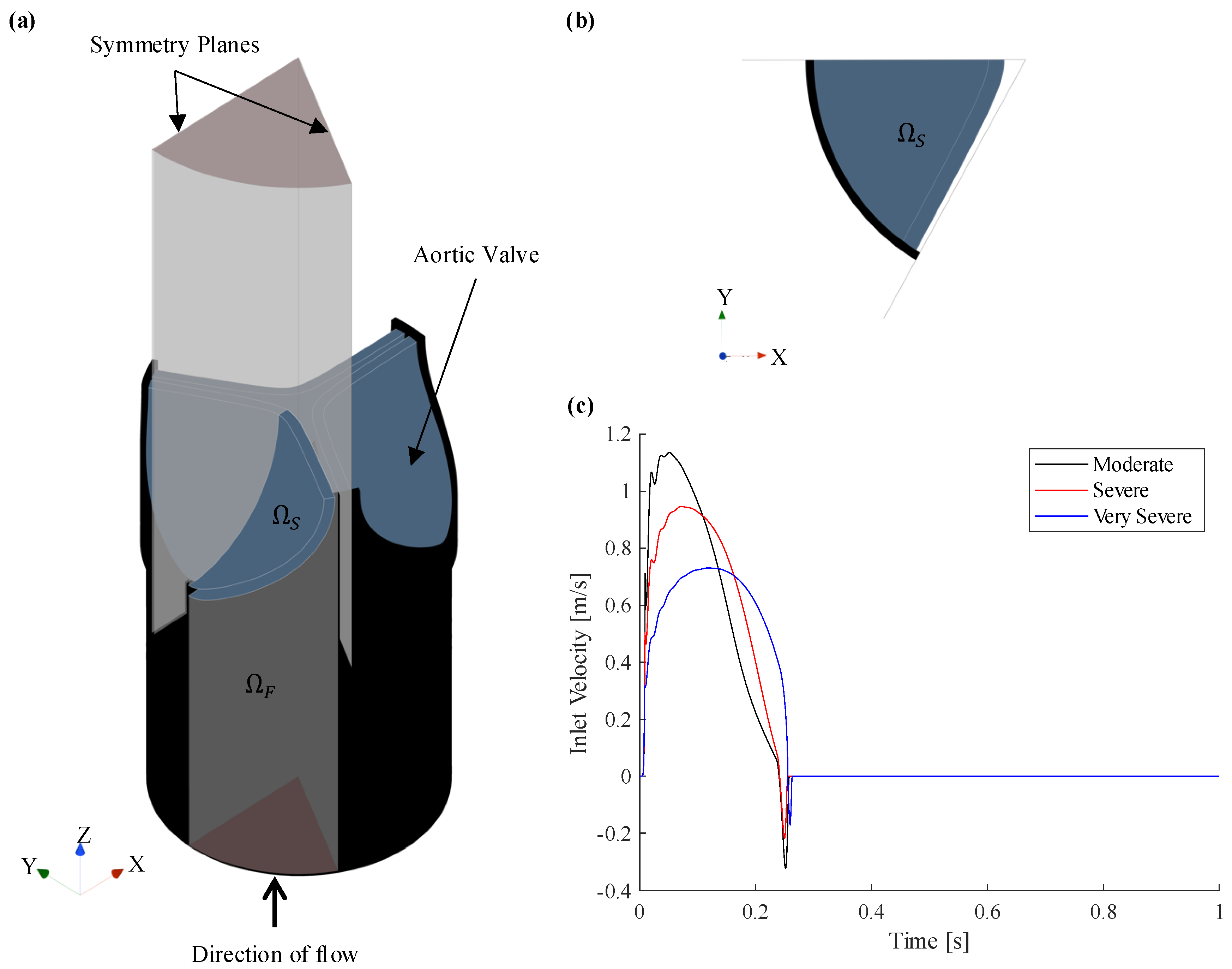
Figure 2.
Leaflet thickening and commissural fusion evident in the moderate (a) calcific, and (b) rheumatic AS valve models.
Figure 2.
Leaflet thickening and commissural fusion evident in the moderate (a) calcific, and (b) rheumatic AS valve models.
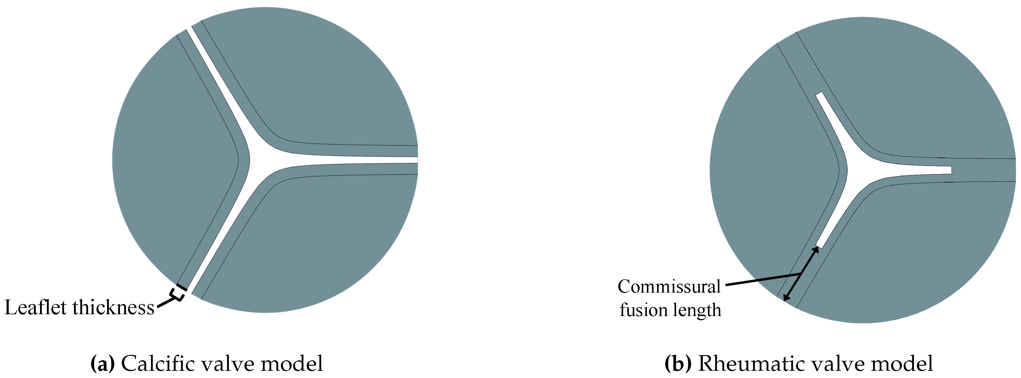
Figure 3.
Model Development. (a) Fluid () and (b) solid () domain.
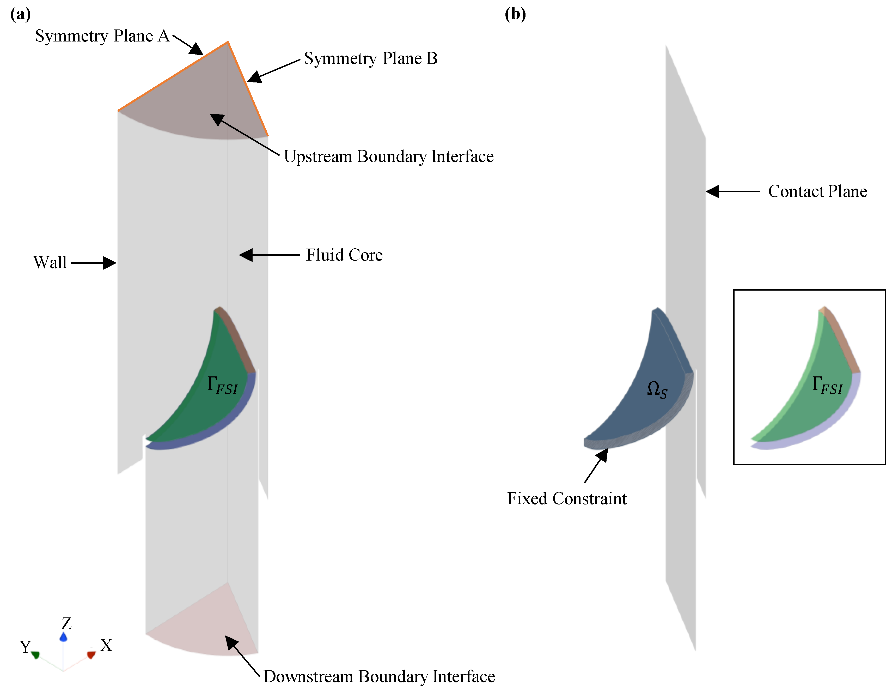
Figure 4.
Calcific Aortic Stenosis. (a) Moderate, (b) severe, and (c) very severe cases showing the area ratio (left), EOA velocity (middle), and TPG (right) profiles over the systolic period.
Figure 4.
Calcific Aortic Stenosis. (a) Moderate, (b) severe, and (c) very severe cases showing the area ratio (left), EOA velocity (middle), and TPG (right) profiles over the systolic period.
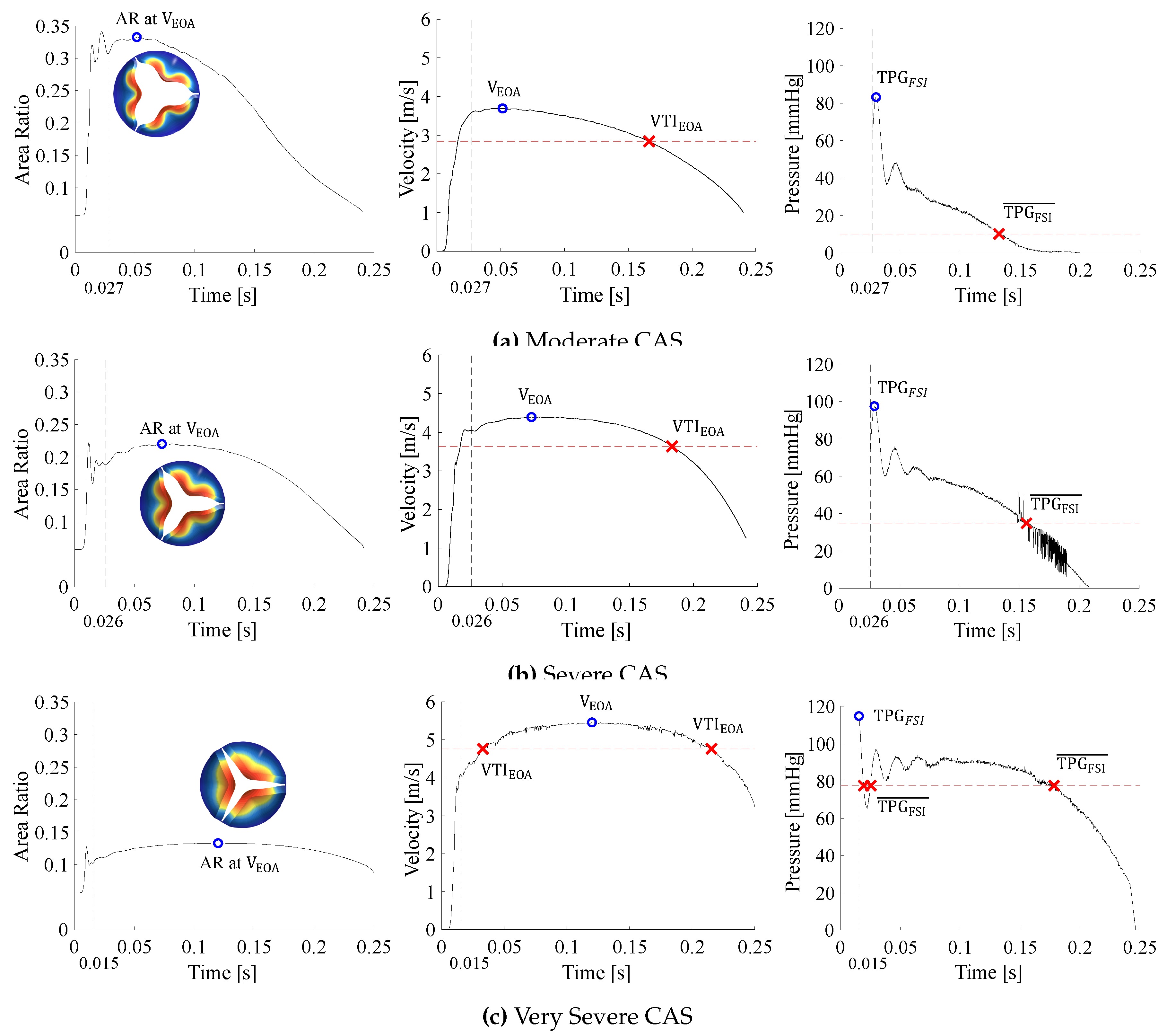
Figure 5.
Rheumatic AS. (a) Moderate, (b) severe, and (c) very severe cases showing the area ratio (left), EOA velocity (middle), and TPG (right) profiles over the systolic period.
Figure 5.
Rheumatic AS. (a) Moderate, (b) severe, and (c) very severe cases showing the area ratio (left), EOA velocity (middle), and TPG (right) profiles over the systolic period.
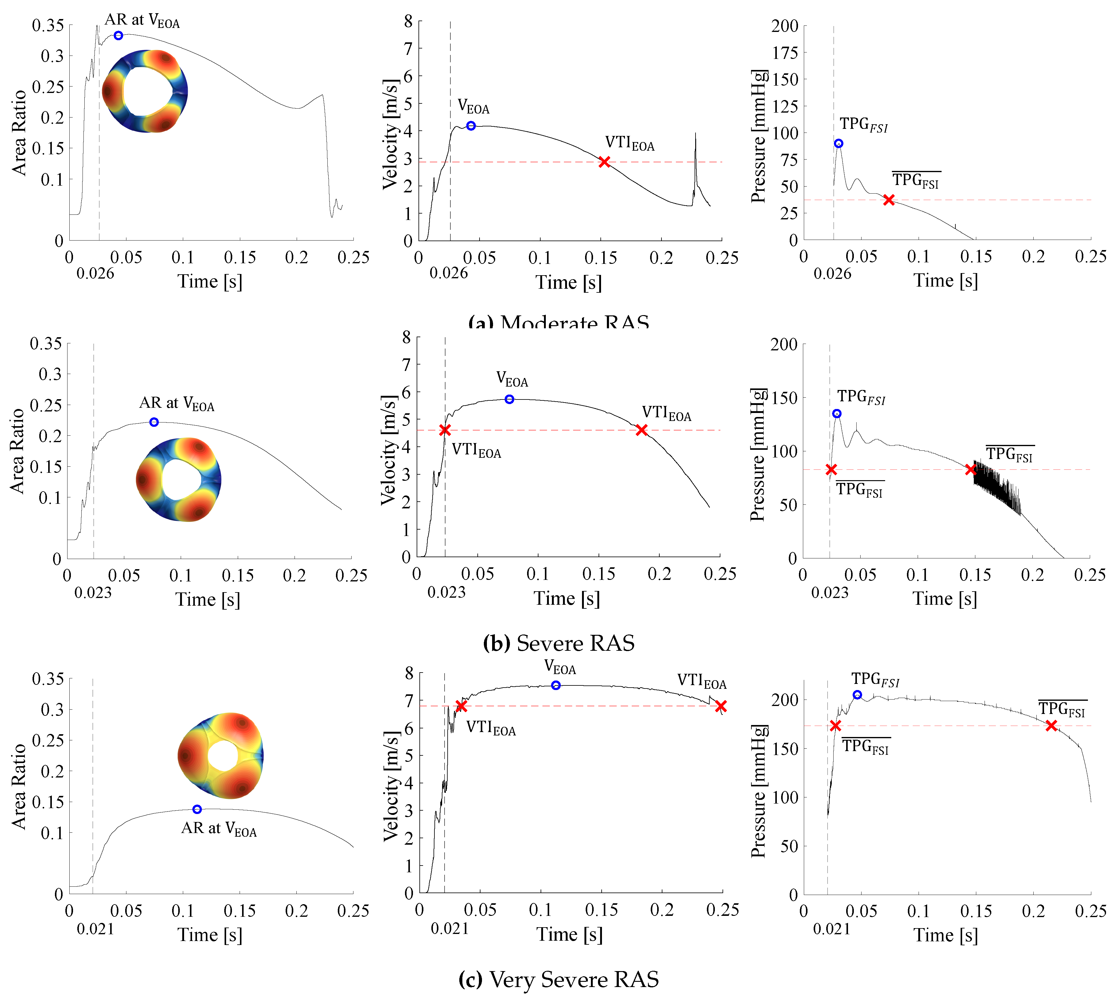
Figure 6.
Moderate CAS and RAS peak systole velocity contour (left) and pressure gradients vs volume flow (right). (a) Moderate Calcific, and (b) Moderate Rheumatic.
Figure 6.
Moderate CAS and RAS peak systole velocity contour (left) and pressure gradients vs volume flow (right). (a) Moderate Calcific, and (b) Moderate Rheumatic.
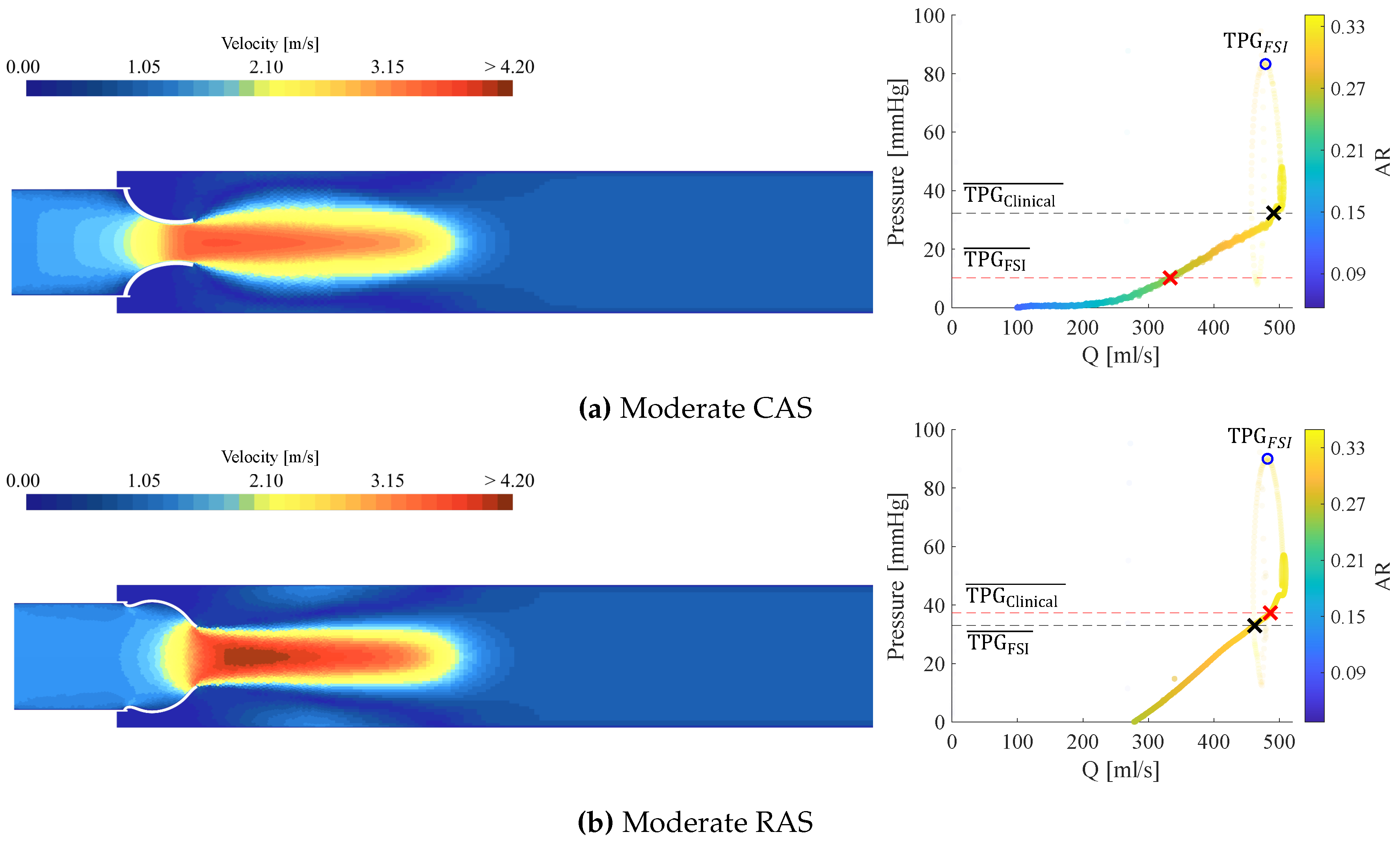
Figure 7.
Severe CAS and RAS peak systole velocity contour (left) and pressure gradients vs volume flow (right). (a) Moderate Calcific, and (b) Moderate Rheumatic.
Figure 7.
Severe CAS and RAS peak systole velocity contour (left) and pressure gradients vs volume flow (right). (a) Moderate Calcific, and (b) Moderate Rheumatic.
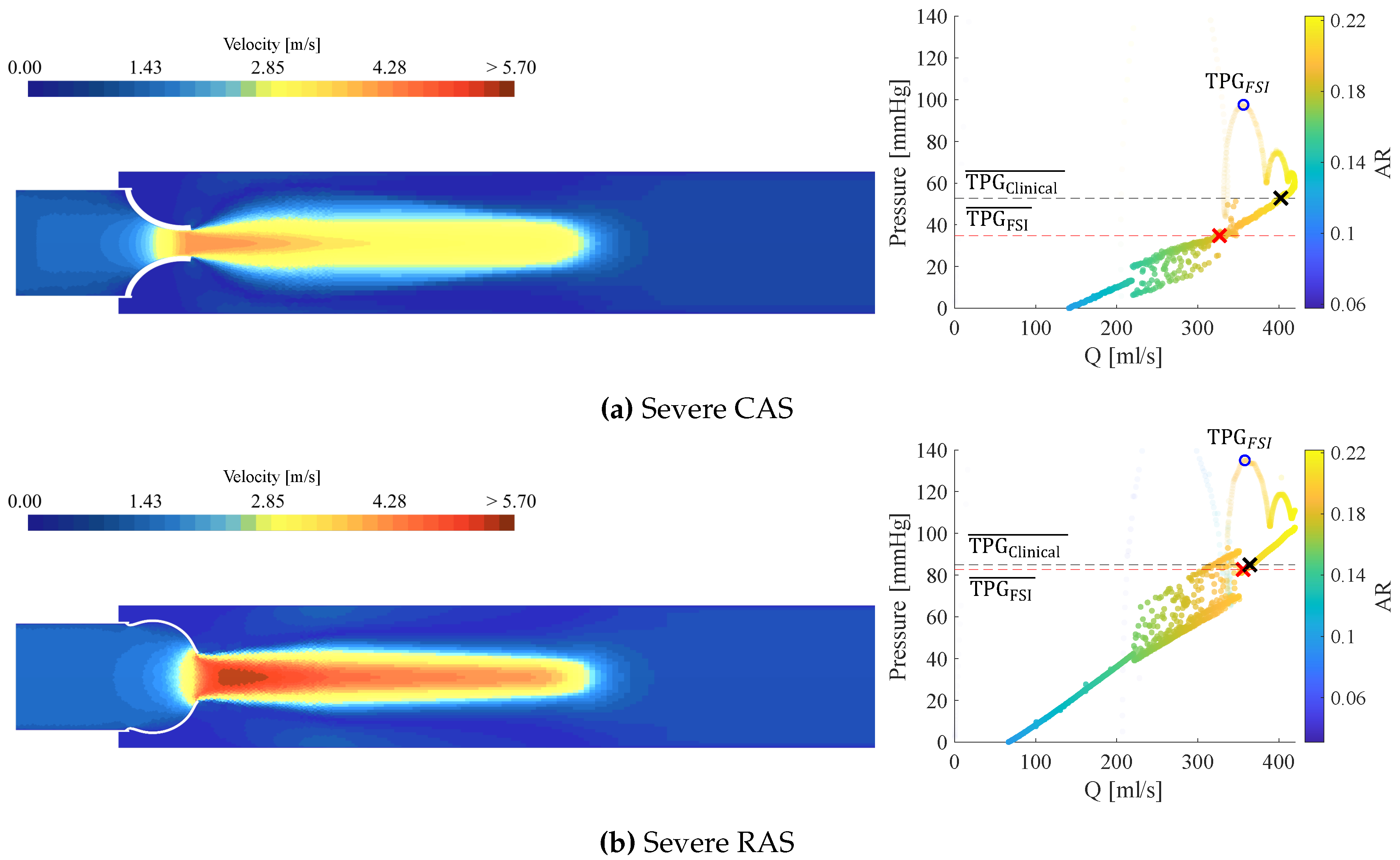
Figure 8.
Very Severe CAS and RAS peak systole velocity contour (left) and pressure gradients vs volume flow (right). (a) Moderate Calcific, and (b) Moderate Rheumatic.
Figure 8.
Very Severe CAS and RAS peak systole velocity contour (left) and pressure gradients vs volume flow (right). (a) Moderate Calcific, and (b) Moderate Rheumatic.
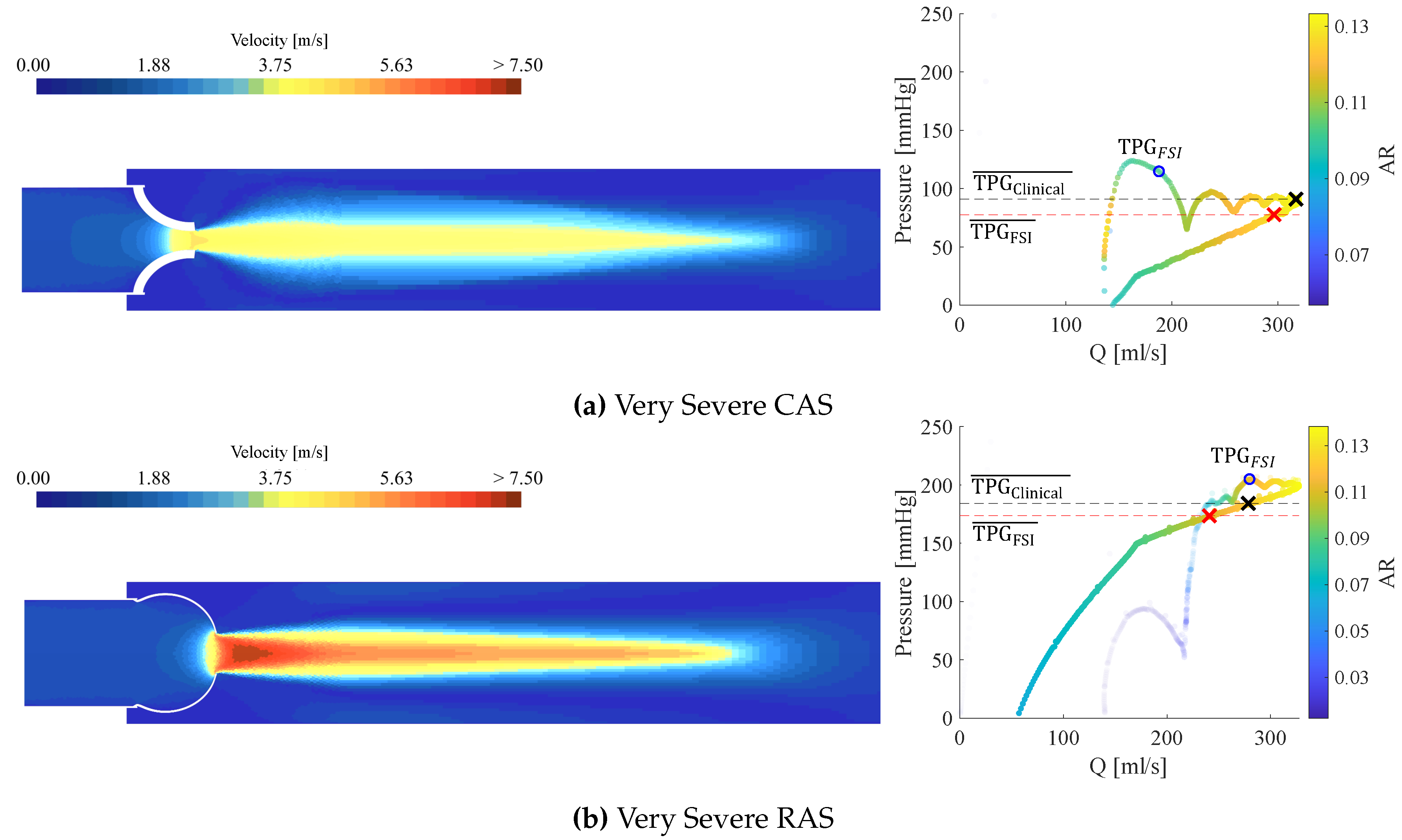

Table 1.
Moderate, severe and very severe CAS and RAS valve model characteristics at peak systolic flow conditions.
Table 1.
Moderate, severe and very severe CAS and RAS valve model characteristics at peak systolic flow conditions.
| Type | Severity | Leaflet thickness [mm] | Commissural fusion length [mm] | AVA [cm2] | AR |
|---|---|---|---|---|---|
| Moderate | 0.896 | - | 1.494 | 0.330 | |
| CAS | Severe | 1.180 | - | 0.992 | 0.219 |
| Very Severe | 1.950 | - | 0.604 | 0.134 | |
| Moderate | 5.05 | 1.516 | 0.335 | ||
| RAS | Severe | 0.650 | 7.75 | 1.004 | 0.222 |
| Very Severe | 10.65 | 0.626 | 0.138 |
Table 2.
Mesh Independence Study.
| Total Cell Count | Peak Velocity GCI | Mean TPG GCI | ||||
|---|---|---|---|---|---|---|
| MC | 219,715 | 1.85 | 1.18 | |||
| SC | 161,259 | 0.74 | 0.02 | |||
| VSC | 135,160 | 0.01 | 0.29 | |||
| MR | 189,563 | 0.82 | 0.18 | |||
| SR | 199,343 | 0.28 | 0.15 | |||
| VSR | 196,378 | 1.17 | 0.31 | |||
Table 3.
Comparison between RAS and CAS simulation results for moderate, severe and very severe stenosis
Table 3.
Comparison between RAS and CAS simulation results for moderate, severe and very severe stenosis
| Flow Parameters | Peak | Mean | |||||||
|---|---|---|---|---|---|---|---|---|---|
| [ | [ | [ | [ | [ | [ | [ | [ | [ | |
| MC | 298 | 1.41 | 3.69 | 40.5 | 83.3 | 54.5 | 2.84 | 10.2 | 32.3 |
| SC | 297 | 2.10 | 4.39 | 60.2 | 97.5 | 77.2 | 3.63 | 34.9 | 52.8 |
| VSC | 260 | 2.74 | 5.46 | 90.0 | 114.8 | 119.1 | 4.77 | 77.6 | 90.9 |
| MR | 300 | 1.51 | 4.18 | 53.0 | 90.0 | 70.0 | 2.87 | 37.3 | 33.0 |
| SR | 301 | 3.65 | 5.73 | 105.0 | 135.0 | 131.2 | 4.61 | 82.8 | 85.0 |
| VSR | 266 | 6.57 | 7.54 | 200.3 | 207.0 | 227.3 | 6.79 | 173.6 | 184.2 |
Disclaimer/Publisher’s Note: The statements, opinions and data contained in all publications are solely those of the individual author(s) and contributor(s) and not of MDPI and/or the editor(s). MDPI and/or the editor(s) disclaim responsibility for any injury to people or property resulting from any ideas, methods, instructions or products referred to in the content. |
© 2025 by the authors. Licensee MDPI, Basel, Switzerland. This article is an open access article distributed under the terms and conditions of the Creative Commons Attribution (CC BY) license (http://creativecommons.org/licenses/by/4.0/).
Copyright: This open access article is published under a Creative Commons CC BY 4.0 license, which permit the free download, distribution, and reuse, provided that the author and preprint are cited in any reuse.


