
Submitted:
21 April 2025
Posted:
22 April 2025
You are already at the latest version
Abstract
A common test configuration used to produce mixed mode I/II in composite materials is the Asymmetric Double Cantilever Beam (ADCB), which consists of two sublaminates with different thickness or elastic properties. This situation usually occurs in bimaterial adhesive joints. During this test, the sample undergoes rotation. In this work, the influence of the rotation of the ADCB samples on the calculation of the energy release rate (ERR) in modes I and II has been studied. When the rotation of the specimen is not negligible, it is important to take this rotation into account in the calculation of modes I and II. This study has been developed using the Finite Element Method (FEM). Several models with different degrees of asymmetry (different thickness ratio and/or elastic modulus ratio) and different applied displacements were prepared to obtain different degrees of rotation during the test. As is known, the concept of modes I and II refers to the components of the energy release rate calculated in the direction perpendicular and tangential to the delamination plane respectively. If the model suffers large rotation during the application of the load, this nonlinearity must be considered in the calculation of the mode partition I/ II. In this work, appreciable differences have been observed in the values of modes I and II depending on their calculation in a global system or a local system that rotates with the sample. Currently, this correction is not usually implemented in finite element calculation codes or in analytical developments. The purpose of this article is to draw attention to this aspect when the rotation of the specimen is not negligible.
Keywords:
FEM
; Composite laminate
; Interlaminar fracture toughness
; Mixed mode
; Delamination
; CFRP
; ADCB
1. Introduction
Because fibre reinforced thermoset matrix composites are made up of sheets, delamination failure is one of the factors that limit the service life of these materials. Crack initiation and growth can take place in pure modes I, II and III. However, in most real situations a combination of these modes is usually observed.
The double cantilever beam (DCB) test configuration is usually used to obtain pure mode I and the end notch flexure (ENF) is commonly used to obtain pure mode II. These test procedures are elevated to the status of international standards [1,2,3].
On the other hand, there are several test procedures developed in the scientific literature to obtain pure mode III, although there is no scientific consensus to elevate any of them to international standard status. Some of these methods are the Split Cantilever Beam (SCB), Crack Rail Shear (CRS), Edge Crack Torsion test (ECT) and Longitudinal Semi Fixed Beam (LHFB) [4,5,6,7,8,9].
One of the most studied mixed modes in the scientific literature is mode I/II. The standardized Mixed Mode Bending (MMB) test method allows generating a mixed mode I/II at the crack tip [10,11]. In this test configuration, mode I is introduced by means of an opening movement, as in the DCB test, and mode II is produced by means of the specimen flexure (as in ENF test) (see Figure 1).
Another alternative test method to generate a mixed mode I/II is the Asymmetric Double Cantilever Beam test (ADCB) [12,13,14]. In this test configuration both sublaminates have different stiffness. This is the situation when we have sublaminates with different thickness and/or different elastic properties (e.g. bimaterial bonded joints). In this situation, a mixed mode I/II is generated at the crack tip. ADCB test specimens and fittings are as simple as in pure mode I tests (DCB). The ADCB test configuration allows generating mixed modes at the crack tip with predominance of mode I
Other test methods to obtain mixed modes I/II are based on the ENF test, as the Single Leg Bending (SLB) and Asymmetric Single Leg Bending (ASLB) tests [15,16].
There are other test configurations developed in the scientific literature to produce mixed mode I/II at the crack tip. This is the case of the Prestressed End-Notched Flexure (PENF) test (Figure 2) proposed by Szekrényes [17]. In this test configuration, mode I is introduced by means of a rod inserted between both sublaminates, and mode II is produced by the specimen flexure.
This test is simple to perform, as bonding hinges in the sample is not required. Boyano et al. studied the influence of different rod positions and diameters on the mixed mode at the crack tip [18].
The analytical determination of GI and GII is not simple when mixed mode is present at the crack tip. There are several analytical methods developed in the scientific literature to evaluate mode I/II partition, but there is not always consensus among researchers. [14,19,20,21,22].
The numerical calculation of mode I/II partition is usually carried out using the Virtual Crack Closure Technique (VCCT) [23] and the Cohesive Zone Modelling (CZM) [24,25] available in commercial FEM programs.
VCCT numerical calculations are usually carried out in global coordinates without taking into account the possible rotation of the specimen during the test. The same situation usually occurs with the analytical developments.
This article aims to draw attention to the fact that, if the ADCB specimen rotates in a non-negligible way during the test, the fact of not taking said rotation into account in the projection of the forces and displacements, can give rise to an appreciable error in the decomposition of modes I and II.
2. Materials and Methods
In this work, the ANSYS® 2024 Academic Research package has been used to study by FEM the influence of the specimen rotation on the ERR decomposition in modes I and II (GI and GII) in ADCB specimens.
As mentioned above, the concept of modes I and II refers to the components of the energy release rate calculated in the direction perpendicular and tangential to the delamination plane respectively. To correctly calculate GI and GII, the components of the forces and displacements involved in the energy calculation must be projected in directions perpendicular and tangential to the delamination plane (xL-yL coordinate system) (see Figure 3).
In this study, two coordinate systems are defined: a global coordinate system (GCS) (xG-yG), with the xG-axis aligned with the crack plane when the specimen is unloaded, that remain horizontal during the test, and a local coordinate system (LCS) (xL-yL) that rotates with the crack plane while loading the sample. Therefore, the xL-axis is always aligned with the crack during the test (see Figure 3).
If the rotation of the specimen during the test is large, the difference in the calculations obtained using both coordinate systems may be non-negligible. As shown in Figure 3, during the ADCB test, when the sublaminates have a significant difference in stiffness, an appreciable rotation of the specimen occurs.
To carry out this study, several ADCB models were prepared with different thickness ratios (h1/h2) in order to obtain different degrees of modes I/II (see Figure 4).
A constant displacement δ was applied to all models on the sample lips. GI and GII were then calculated using forces and displacements in global and local coordinates.
FEM packages usually implement the Virtual Crack Closure Technique (VCCT) in order to calculate GI and GII. The VCCT method calculates the energy released by the opening of the nodes during crack growth in a single step. This is a simplification since the force is calculated at the crack tip when the crack has already grown, but it is a very efficient calculation method.
In the VCCT method [26] (see Figure 5), the components of forces and displacements are calculated in the same step using two different node pairs. Forces are calculated in nodes 2i-2i’ and displacements are calculated in nodes 1i-1i’. This approximation is valid providing that forces at the crack tip before and after the crack extension are similar when the crack increment (element size) is small enough.
The calculation using the VCCT method was performed with the CINT function of the Ansys program (CINT,TYPE,VCCT) [27].
GI and GII are then calculated as follows:
B is the specimen width. The subscript i takes into account a 3D system with n nodes along the crack front.
The VCCT method, implemented in this commercial FEM package, uses the global coordinate system to perform de calculations (the coordinate system is not updated as the crack plane rotates).
In this article, a similar method without simplification (TSEM) is also used. In this method, loads are calculated in the first step and the corresponding displacements are calculated in a second step once the nodes have separated. Loads and displacements are therefore calculated in the same node pair (nodes 1i-1i’ in Figure 6 and Figure 7) [28,29].
GI and GII are calculated by means of TSEM as follows:
Therefore, data needs to be collected in two successive calculation steps to perform the energy calculations. This method was applied using both global (Figure 6) and local coordinate systems (Figure 7).
This method is not originally implemented in the ANSYS FEM package. Therefore, a script programmed in APDL (Ansys Parametric Design Language) was specifically developed for this purpose in this work. This method was programmed using local and global coordinates. In this way, it will be possible to compare results taking or not into account the rotation of the coordinate system. Moreover, TSEM results in global coordinates can be compared with the VCCT originally implemented in Ansys (and most commercial FEM packages), as they are equivalent when the element size ahead of the crack tip is small enough.
3. Model Calibration
A 2D FEM model was prepared using ANSYS® 2024 Academic Research. The element used was the 2D structural PLANE182 with the plane strain option.
A first model was prepared to optimize the element size near the crack tip. This model had the following dimensions:
- L=150 mm
- a0=50 mm
- h1=4.6 mm
- h2=1.4 mm
A regular mesh was implemented with the same size before and after the crack tip (Figure 8). Several runs using the TSEM procedure were performed in global coordinates with different element sizes to optimize the model. The mesh was refined around the crack tip until results variation was negligible. The elements were nearly squared.
A displacement of δ=8 mm was applied to the sample lips.
Finally, the element size in the vicinity of the crack tip was set to 0.100 mm for the following studies. A thinner mesh would produce a negligible change in ERR values (0.1%).
Another issue to take in consideration is whether the calculations should be performed in a linear or non-linear way due to sample rotation.
To perform VCCT crack growth simulations, the Ansys manual specifies the assumption that the model undergoes a small deformation (or a small rotation), and so, the calculation is performed with the option NLGEOM, OFF [27]. This option causes the calculation to be performed by a linear procedure, without taking into account possible non-linear effects. There are three possible sources of non-linearities: material non-linearity, contacts and large displacements or deformations. This is an issue to take into account, as asymmetric specimens, may show non negligible rotations.
Large displacements or rotations can cause the stiffness of the system to change as the load is applied to the sample lips. If the change in stiffness of the system during the loading process is not negligible, it must be taken into account as a source of non-linearity in the calculations.
Two runs were performed to investigate the influence of the calculation procedure (linear or non-linear procedure).
The model used was the same as the one used for element size optimisation. In this case, a displacement of 4.5 mm was applied to the sample. This displacement is assumed to be close to the critical displacement of the material for this configuration. The obtained results are shown in Table 2.
The units of the applied load were set as N assuming a width of 1 mm (a 2D model has been used). In this Table, the total energy release rate (GT) was calculated in two ways: as the sum of GI and GII previously calculated by means of the TSEM procedure, and, directly, by means of the overall loss of elastic energy divided by the area of the crack increment (one element length). In mathematical form:
Both procedures give similar results for both calculation procedures (linear and non-linear), but, as can be seen in the Table above, linear calculations give identical results irrespective of the procedure used to calculate GT (0.382 N/mm).
This model was also used to compare both FEM solution procedures with the analytical Corrected Beam Theory proposed by ISO 15024 [1] standard, equivalent to the Modified Beam Theory in ASTM D 5528 [2]. Although this formulation is designed to calculate GI in symmetric samples, it can be also used to calculate GT in asymmetric samples as it was demonstrated in [30].
where,
- P: applied load
- δ: applied displacement
- B: sample width
- a: crack length
- Δ: crack length correction
Δ takes into account that the beam is not perfectly built in. This parameter is calculated by plotting the cube-root of the compliance as a function of delamination length. The extrapolation of the linear fit through the data in the plot yields Δ as the x-intercept [1]. This was done by analysing various models with h1=4.6 mm, h2=1.4 mm and different initial crack lengths by FEM. Once Δ was obtained, a new model with a0= 50 mm and an applied displacement δ=4.5 mm was analysed. Table 3 shows the obtained results calculated following equations 3 and 4, and additionally, with the analytical equation 6. These calculations were performed using linear and non-linear solutions.
As can be seen in this Table, both solution procedures (linear and non-linear) yield similar results and agree very well with the analytical solution. The time needed to solve the model with each procedure is very similar since a 2D model is used.
Because the solution time is similar between the two procedures, non-linear solution will be used in the following calculations to take into account the small non-linearities present in this model (the stiffness matrix of the model changes slightly as the displacement is applied).
4. Influence of the Sample Rotation
Once the base model has been optimized, several runs were performed increasing the applied displacement with the same model used in the previous studies. This causes the sample to progressively increase its rotation (see Figure 9).
These models were analysed using TSEM in local and global coordinates by means of the APDL script developed specifically for this purpose and also, using the VCCT procedure available in ANSYS by means of the CINT,TYPE,VCCT function. As commented before, this function, implemented in the Ansys package, uses only global coordinates. Results are shown in Table 4, Table 5 and Table 6.
Comparing Table 4 and Table 5, we can see that both procedures yield practically identical results and match the partition values GI/GT and GII/GT. These results were expected as both procedures perform the calculations in global coordinates, and they are very similar: only differs in the node where the force is calculated (one element length away from each other). The two procedures tend to converge on each other as the size of the element at the crack tip decreases.
We can also observe in Table 4 and Table 5, that as the rotation of the sample increases, the partition values (GI/GT - GII/GT) change from 75%-25% for δ=1 mm to 61%-39% for δ=20 mm. This represents a change of 19% in the GI/GT values and 58% in the GII/GT values. This change in the partition values can be attributed to the appreciable rotation of the sample as the displacement increases. We must remember that, in these tables, forces and displacements are calculated always horizontal and vertical (according to the GCS) independently of the sample rotation.
On the other hand, Table 6 shows the calculations using forces and displacements always perpendicular and parallel to the crack plane, this is, considering the rotation of the sample (LCS).
This procedure gives rise to different results from the previous ones using GCS and the difference between results increases as the rotation of the specimen increases. Using local coordinates, GI/GT - GII/GT ratios change from 76%-24% for δ=1 mm to 79%-21% for δ=20 mm as the displacement increases. As we can see, the ERR partition has a much smaller change as the sample increases rotation. In this case, the small change in the partition values could be influenced, among other issues, by the shortening of the distance a0 due to sample rotation and arm flexure.
Finally, as it was expected, the total energy GT dissipated when the crack grows is the same for a given displacement, independently of the coordinate system used (Table 5 and Table 6). Obviously, the total energy dos not dependent on the coordinate system used to calculate GI and GII.
We can evaluate ERR modes I and II in global coordinates (GGI, GGII) as a function of modes I and II in local coordinates (GLI, GLII) (Figure 10) or vice versa as follows:
and adding equations 9 and 10:
In Table 7 we can see the differences between the calculated values of GI and GII using GCS and LCS for different displacements applied to the sample (calculated based on results in Table 5 and Table 6).
As expected, we can see that, for small rotations the difference between calculations in GCS and LCS is low, but if the rotation of the sample is significant, the error made when calculating in GCS can be very significant compared to LCS. For a displacement of only 5 mm, the difference obtained in GI and GII values is 4% and 14% respectively when calculating in GCS and LCS. And for a displacement of 10 mm, de differences in GI and GII values reach 10% and 35% respectively. This should be considered in the numerical and analytical calculations when the sample rotation is large. That is, when the applied displacement, and/or the difference in the stiffness of both sublaminates is considerable.
As stated above, another source of non-linearity is the displacement of the crack tip node as the applied load increases (see Table 7). For δ=20 mm, the equivalent crack length (measured perpendicular to the loading axis) shortens 1.8 mm making the sample response stiffer.
Next, some models were prepared with different h2/h1 and E2/E1 ratios to produce different mixity-modes. The applied load was set to δ=10 mm and the initial crack length was set to a0=50 mm. The obtained results can be seen in Table 8.
The ratio E1h12/E2h22 has been included in this Table to give an idea of how far each configuration is from pure mode I condition, assuming that pure mode I condition is reached when the longitudinal strain distributions at both sublaminates interfaces are identical [31] (Figure 11 and Figure 12). Therefore, pure mode I condition is achieved as follows:
Figure 13 shows the rotation of the sample with h2/h1=0.2 compared to the symmetric sample for δ=20 mm.
Finally, crack growth calculations were performed in order to evaluate the influence of the method used (LCS or GCS) on the obtained critical load.
To determine the crack onset and subsequent crack growth, it is necessary to define a fracture criterion. The Benzeggagh-Kenane criterion was assumed [27,32]:
The exponent η was set to 1.45 following [33]
The model was set as follows:
- E1=E2=144,000 MPa
- h1= 5 mm
- h2= 1 mm
- a0= 50 mm
The obtained results are shown in Table 9. As can be seen in this Table, the difference between critical values (both displacement and load) is in the order of 4% in this case. The calculation performed at LCS is on the safe side as it predicts a crack growth onset at lower load and displacement. Figure 14 shows the corresponding load-displacement curves.
5. Conclusions
The ADCB configuration is, essentially, a DCB specimen with different sublaminate thickness and/or different elastic modulus. This is the case, for example, in bonded joints with dissimilar adherents.
When the ADCB specimen suffers large rotations during the application of the load, this nonlinearity must be considered in the calculation of displacements and forces, both in numerical and analytical procedures. In this work it has been demonstrated that, the difference in the ERR calculations when the angle of rotation of the sample is taken into account or not, can be very significant depending on the sample configuration and the applied displacement to the sample lips.
For a displacement of only 5 mm, the difference obtained in GI and GII values is 4% and 14% respectively when calculating in GCS and LCS. And for a displacement of 10 mm, de differences in GI and GII values reach 10% and 35% respectively.
When performing crack growth calculations, the difference between critical values (both displacement and load at the crack onset) can be in the order of 4%.
In the case of large rotation, it must be ensured that the ERR in modes I and II is calculated using the displacements and forces projected according to a coordinate system that rotates with the crack plane, that is, perpendicular and tangential to the crack plane. This is the case when the applied displacement is large, and/or when the difference in stiffness of the sub-laminates is large.
This correction is not usually implemented in numerical codes or in analytical developments, so this is an issue to take into account when the rotation of the sample is not negligible.
Author Contributions
Conceptualization, JB. and V.M.; formal analysis, JB. and V.M.; investigation JB. and V.M.; methodology, J.B.; software, J.B. and V.M.; validation, J.V. and A.A., writing—original draft preparation, J.B.; writing— review & editing V.M. All authors have read and agreed to the published version of the manuscript
Funding
This research received no external funding
Data Availability Statement
The original contributions presented in this study are included in the text. Further inquiries can be directed to the corresponding author.
Conflicts of Interest
The authors declare no conflicts of interest.
Abbreviations
The following abbreviations are used in this manuscript:
| FEM | Finite Element Modelling |
| DCB | Double Cantilever Beam |
| ENF | End Notched Flexure |
| ADCB | Asymmetric Double Cantilever Beam |
| VCCT | Virtual Crack Closure Technique |
| TSEM | Two Step Extension Method |
| GCS | Global Coordinate System |
| LCS | Local Coordinate System |
References
- ISO 15024 Fibre-Reinforced Plastic Composites-Determination of Mode I Interlaminar Fracture Toughness, GIC, for Unidirectionally Reinforced Materials; 2023.
- ASTM D5528/D5528M-21 Standard Test Method for Mode I Interlaminar Fracture Toughness of Unidirectional Fiber-Reinforced Polymer Matrix Composites. 2021. [CrossRef]
- ASTM D7905/D7905M-19e1 Standard Test Method for Determination of the Mode II Interlaminar Fracture Toughness of Unidirectional Fiber-Reinforced Polymer Matrix Composites. 2019. [CrossRef]
- Donaldson, S.L. Mode III Interlaminar Fracture Characterization of Composite Materials. Compos Sci Technol 1988, 32, 225–249. [Google Scholar] [CrossRef]
- Martin, R.H. Evaluation of the Split Cantilever Beam for Mode III Delamination Testing. Nasa Technical Memorandum 101562 1989. [Google Scholar]
- Becht, G.J.; Gillespie, J.W. Numerical and Experimental Evaluation of the Mode III Lnterlaminar Fracture Toughness of Composite Materials. Polym Compos 1989, 10, 293–304. [Google Scholar] [CrossRef]
- Lee, S. An Edge Crack Torsion Method for Mode III Delamination Fracture Testing. Journal of Composites, Technology and Research 1993, 15, 193.201. [Google Scholar] [CrossRef]
- de Morais, A.B.; Pereira, A.B.; de Moura, M.F.S.F.; Magalhães, A.G. Mode III Interlaminar Fracture of Carbon/Epoxy Laminates Using the Edge Crack Torsion (ECT) Test. Compos Sci Technol 2009, 69, 670–676. [Google Scholar] [CrossRef]
- Bonhomme, J.; Mollón, V.; Viña, J.; Argüelles, A. Finite Element Analysis of the Longitudinal Half Fixed Beam Method for Mode III Characterization. Compos Struct 2020, 232. [Google Scholar] [CrossRef]
- ASTM D6671/D6671M − 22 Standard Test Method for Mixed Mode I-Mode II Interlaminar Fracture Toughness of Unidirectional Fiber Reinforced Polymer Matrix Composites. ASTM International 2022, 1–15.
- John H., Crews; James, R. Reeder A Mixed-Mode Bending Apparatus for Delamination Testing. NASA Technical memorandum 100662 1976, 1000. [Google Scholar]
- Williams, M.L. The Stresses around a Fault or Crack in Dissimilar Media; 1959; Vol. 49;
- Sundararaman, V.; Davidson, B.D. An Unsymmetric Double Cantilever Beam Test for Interfacial Fracture Toughness Determination; Elsevier Science Ltd, 1997; Vol. 34;
- Ducept, F.; Gamby, D.; Davies, P. A Mixed-Mode Failure Criterion Derived from Tests on Symmetric and Asymmetric Specimens;
- Ramírez, F.M.G.; de Moura, M.F.S.F.; Moreira, R.D.F.; Silva, F.G.A. Experimental and Numerical Mixed-Mode I + II Fracture Characterization of Carbon Fibre Reinforced Polymer Laminates Using a Novel Strategy. Compos Struct 2021, 263. [Google Scholar] [CrossRef]
- Szekrényes, A.; Uj, J. Comparison of Some Improved Solutions for Mixed-Mode Composite Delamination Coupons. Compos Struct 2006, 72, 321–329. [Google Scholar] [CrossRef]
- Szekrényes, A. Prestressed Fracture Specimen for Delamination Testing of Composites. Int J Fract 2006, 139, 213–237. [Google Scholar] [CrossRef]
- Boyano, A.; Mollón, V.; Bonhomme, J.; De Gracia, J.; Arrese, A.; Mujika, F. Analytical and Numerical Approach of an End Notched Flexure Test Configuration with an Inserted Roller for Promoting Mixed Mode I/II. Eng Fract Mech 2015, 143, 63–79. [Google Scholar] [CrossRef]
- Valvo, P.S. On the Calculation of Energy Release Rate and Mode Mixity in Delaminated Laminated Beams. Eng Fract Mech 2016, 165, 114–139. [Google Scholar] [CrossRef]
- Williams, J.G. Observations on the Analysis of Mixed Mode Delamination in Composites. In Proceedings of the Procedia Engineering; Elsevier Ltd, 2015; Vol. 114, pp. 189–198.
- Harvey, C.M. Mixed-Mode Partition Theories for One-Dimensional Fracture;
- Wang, S.; Harvey, C.M. Mixed Mode Partition Theories for One Dimensional Fracture. Eng Fract Mech 2012, 79, 329–352. [Google Scholar] [CrossRef]
- Krueger, R. Virtual Crack Closure Technique: History, Approach, and Applications. Appl Mech Rev 2004, 57, 109–143. [Google Scholar] [CrossRef]
- Chaboche, J.L.; Girard, R.; Schaff, A. Numerical Analysis of Composite Systems by Using Interphase/Interface Models. Comput Mech 1997, 20, 3–11. [Google Scholar] [CrossRef]
- Chen, J.; Crisfield, M.; Kinloch, A.J.; Busso, E.P.; Matthews, F.L.; Qiu, Y. Predicting Progressive Delamination of Composite Material Specimens via Interface Elements. Mechanics of Composite Materials and Structures 1999, 6, 301–317. [Google Scholar] [CrossRef]
- Krueger, R. Virtual Crack Closure Technique: History, Approach, and Applications. Appl Mech Rev 2004, 57, 109. [Google Scholar] [CrossRef]
- Fracture Analysis Guide. 3.5. VCCT-Based Crack Growth Simulation. Ansys Release 2023R2; 2023;
- Mollón, V.; Bonhomme, J.; Elmarakbi, A.M.; Argüelles, A.; Viña, J. Finite Element Modelling of Mode I Delamination Specimens by Means of Implicit and Explicit Solvers. Polym Test 2012, 31, 404–410. [Google Scholar] [CrossRef]
- Bonhomme, J.; Argüelles, A.; Viña, J.; Viña, I. Numerical and Experimental Validation of Computational Models for Mode I Composite Fracture Failure. Comput Mater Sci 2009, 45, 993–998. [Google Scholar] [CrossRef]
- Mollón, V.; Bonhomme, J.; Viña, J.; Argüelles, A. Mixed Mode Fracture Toughness: An Empirical Formulation for GI/GII Determination in Asymmetric DCB Specimens. Eng Struct 2010, 32, 3699–3703. [Google Scholar] [CrossRef]
- Wang, W.; Lopes Fernandes, R.; Teixeira De Freitas, S.; Zarouchas, D.; Benedictus, R. How Pure Mode I Can Be Obtained in Bi-Material Bonded DCB Joints: A Longitudinal Strain-Based Criterion. Compos B Eng 2018, 153, 137–148. [Google Scholar] [CrossRef]
- Benzeggagh, M.L.; Kenane, M. Measurement of Mixed-Mode Delamination Fracture Toughness of Unidirectional Glass / Epoxy Composites With Mixed-Mode Bending Apparatus. Compos Sci Technol 1996, 56, 439–449. [Google Scholar] [CrossRef]
- Falcó, O.; Ávila, R.L.; Tijs, B.; Lopes, C.S. Modelling and Simulation Methodology for Unidirectional Composite Laminates in a Virtual Test Lab Framework. Compos Struct 2018, 190, 137–159. [Google Scholar] [CrossRef]
Figure 1.
MMB tests (Mixed Mode Bending)
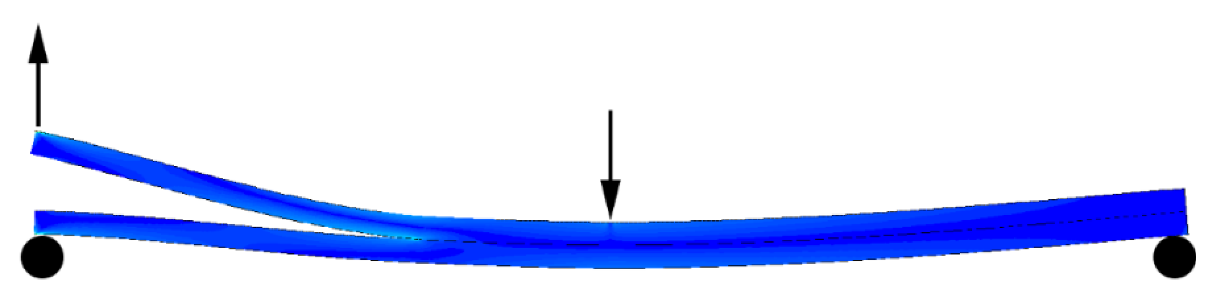
Figure 2.
Prestressed End-Notched Flexure (PENF) test
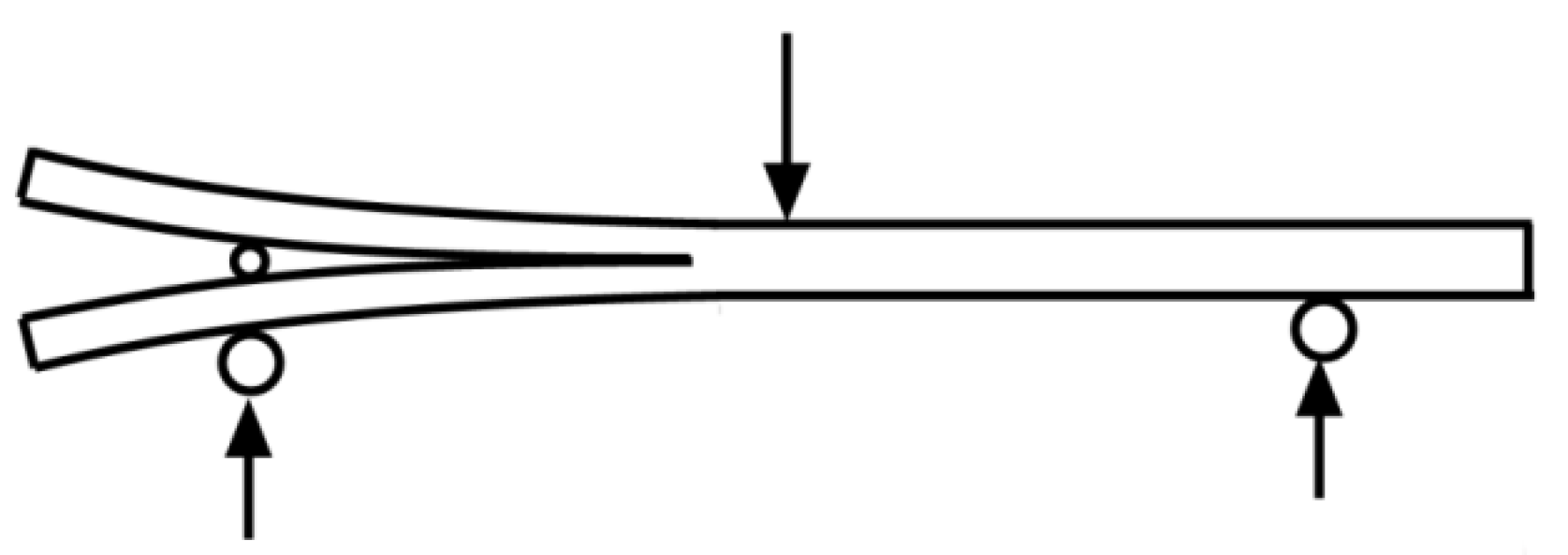
Figure 3.
ADCB specimen and mesh at the crack tip with local (xL-yL) and global (xG-yG) coordinate systems
Figure 3.
ADCB specimen and mesh at the crack tip with local (xL-yL) and global (xG-yG) coordinate systems
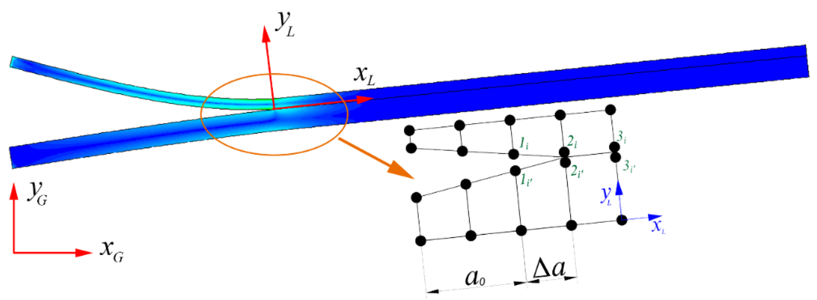
Figure 4.
ADCB. Specimen configuration
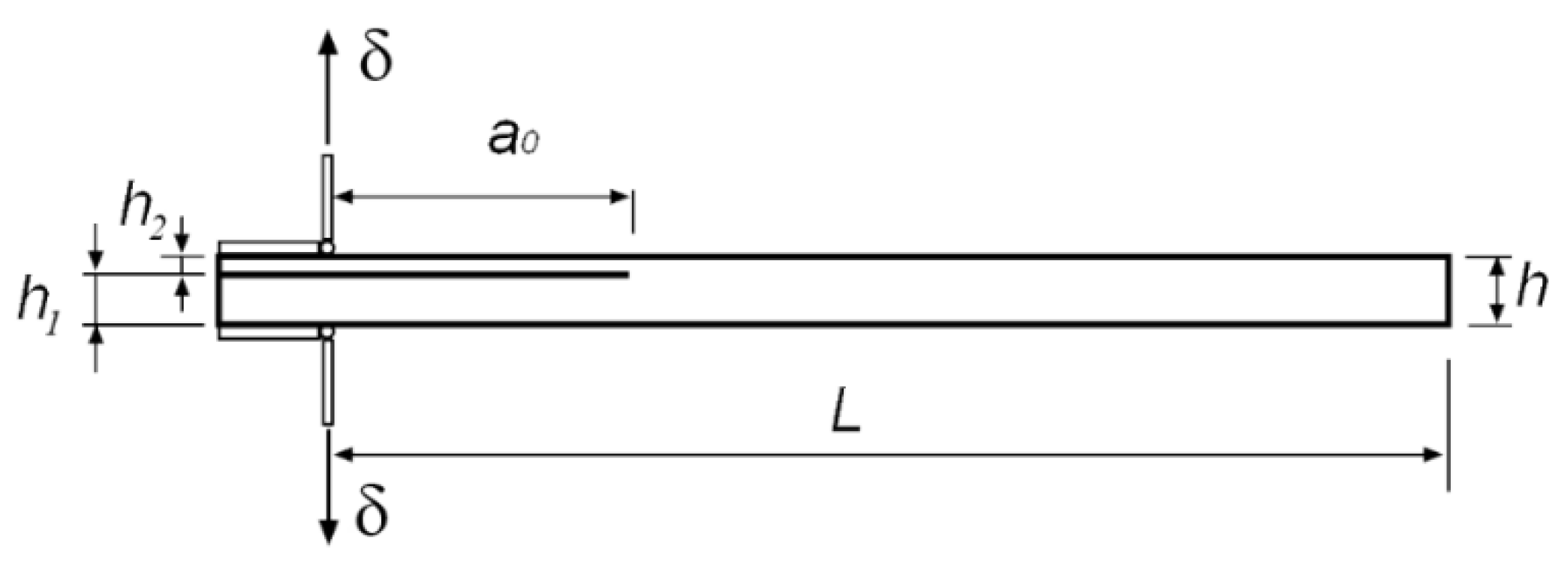
Figure 5.
VCCT method in global coordinate system.
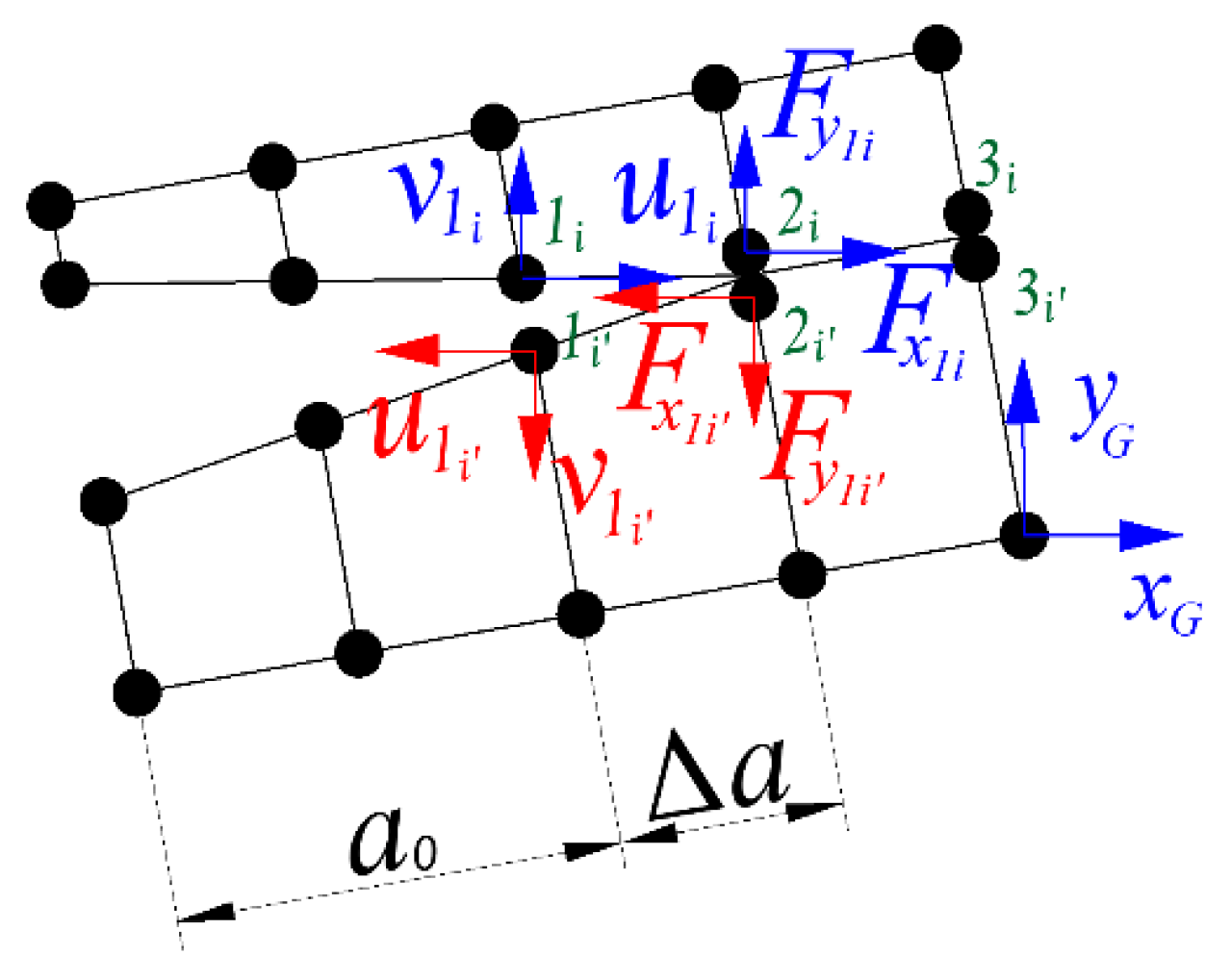
Figure 6.
TSEM method in global coordinate system
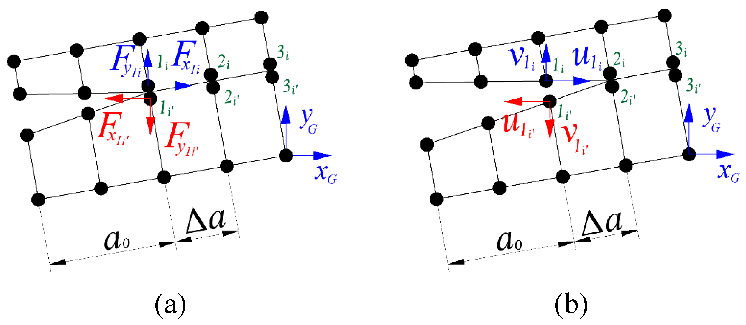
Figure 7.
TSEM method in local coordinate system
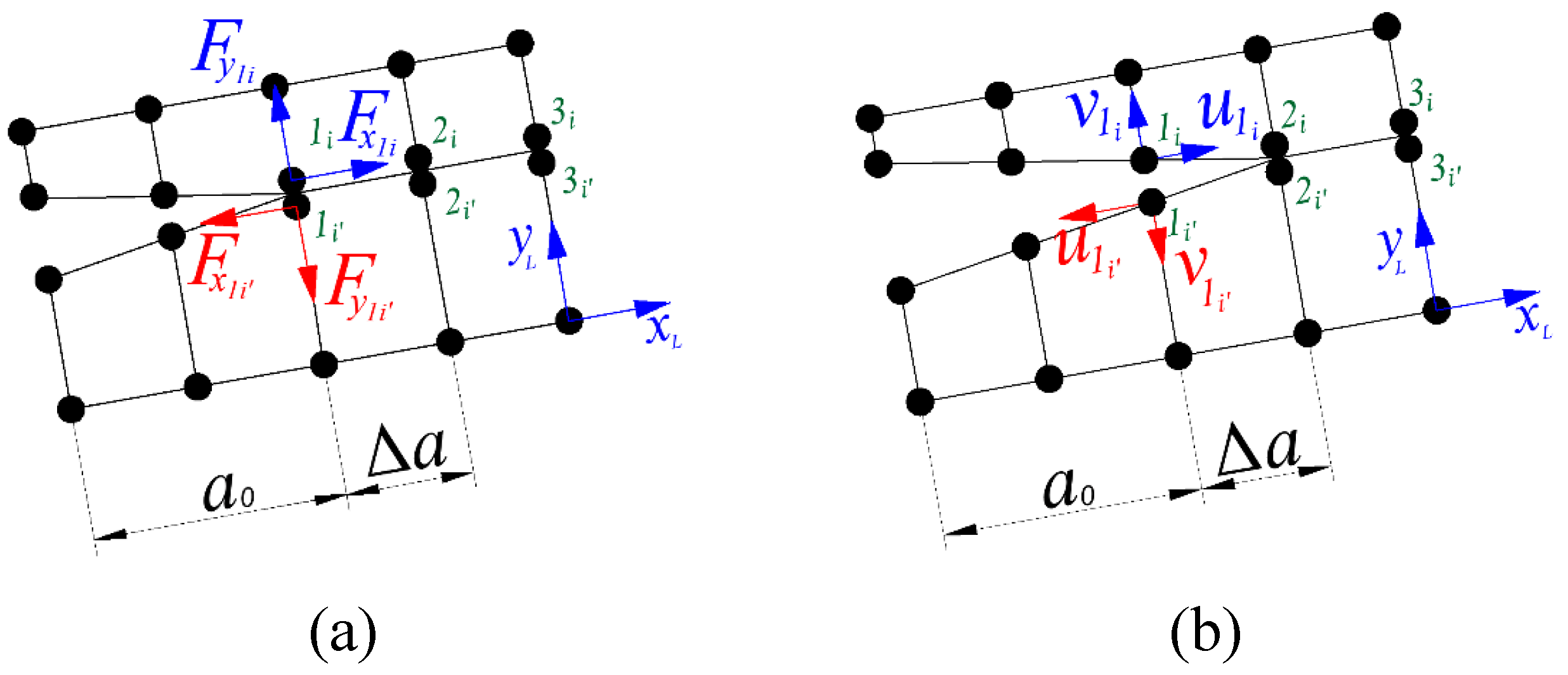
Figure 8.
Mesh near the crack tip
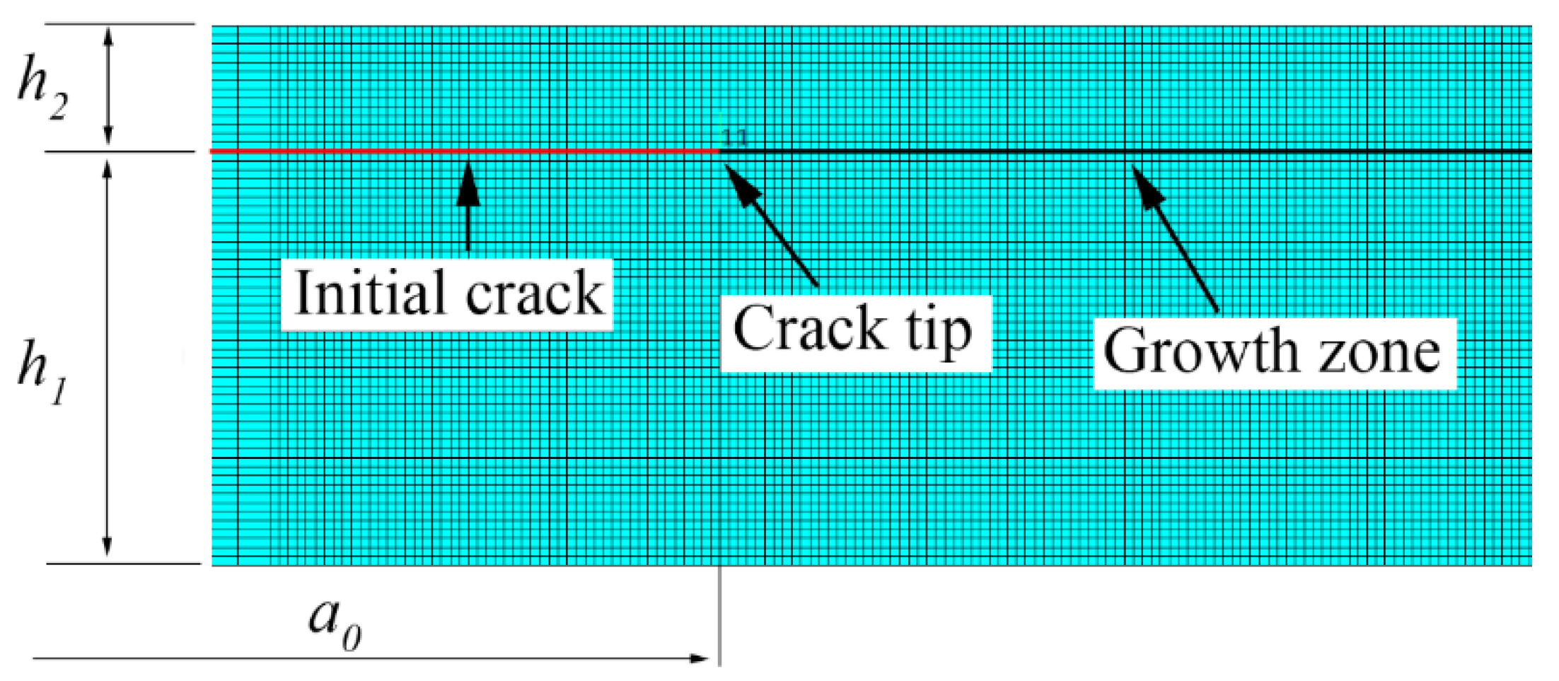
Figure 9.
Deformed sample for different applied displacements. Sample configuration: a0=50 mm, h1=4.6 mm, h2=1.4 mm. Elastic properties: Table 1.
Figure 9.
Deformed sample for different applied displacements. Sample configuration: a0=50 mm, h1=4.6 mm, h2=1.4 mm. Elastic properties: Table 1.
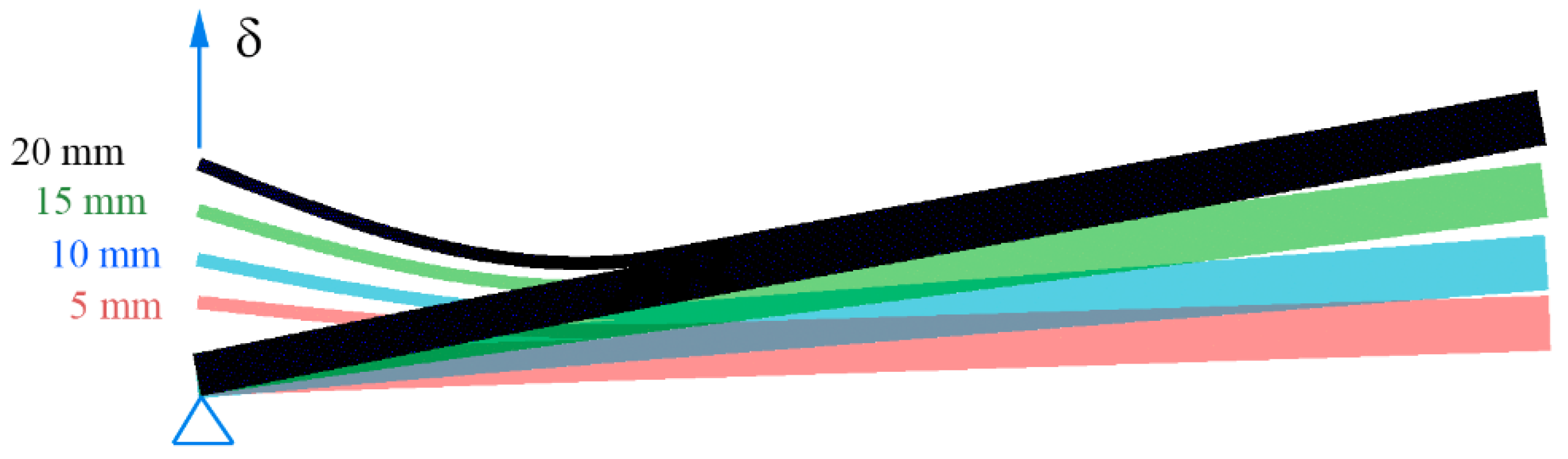
Figure 10.
Coordinate transformation
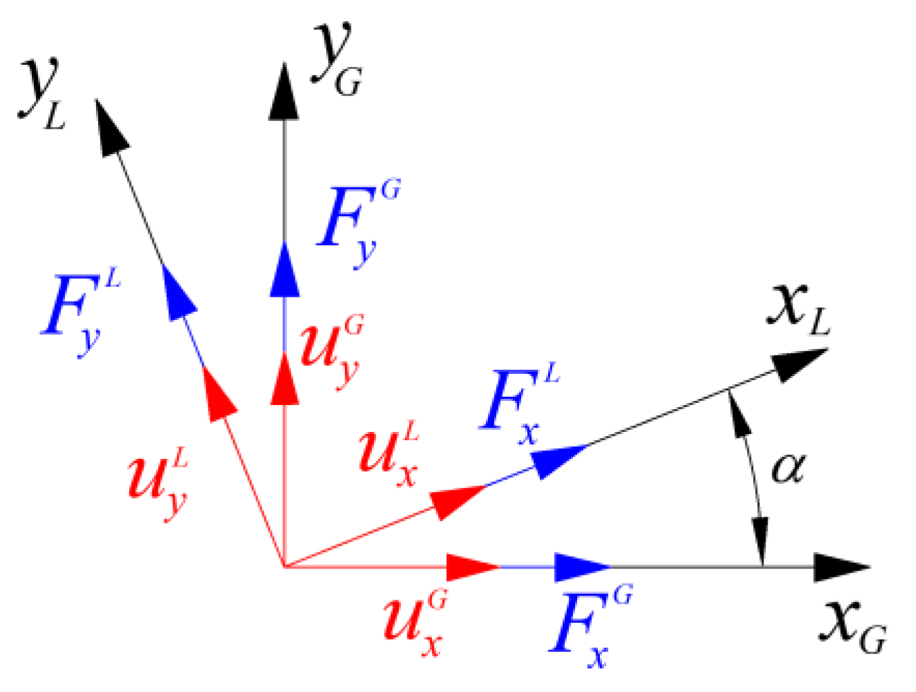
Figure 11.
Displacement near the crack tip
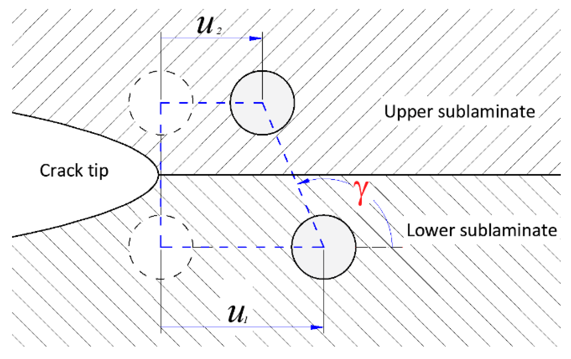
Figure 12.
Mesh deformation near the crack tip
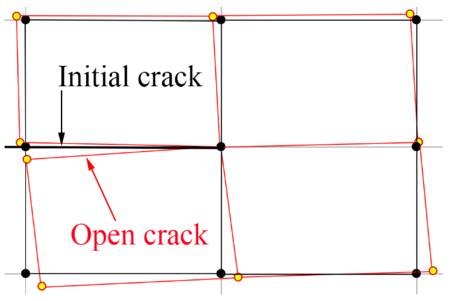
Figure 13.
Deformed sample for different sublaminate stiffness for an applied displacement of 20 mm. Sample configuration: a0=50 mm, Elastic properties: Table 1
Figure 13.
Deformed sample for different sublaminate stiffness for an applied displacement of 20 mm. Sample configuration: a0=50 mm, Elastic properties: Table 1
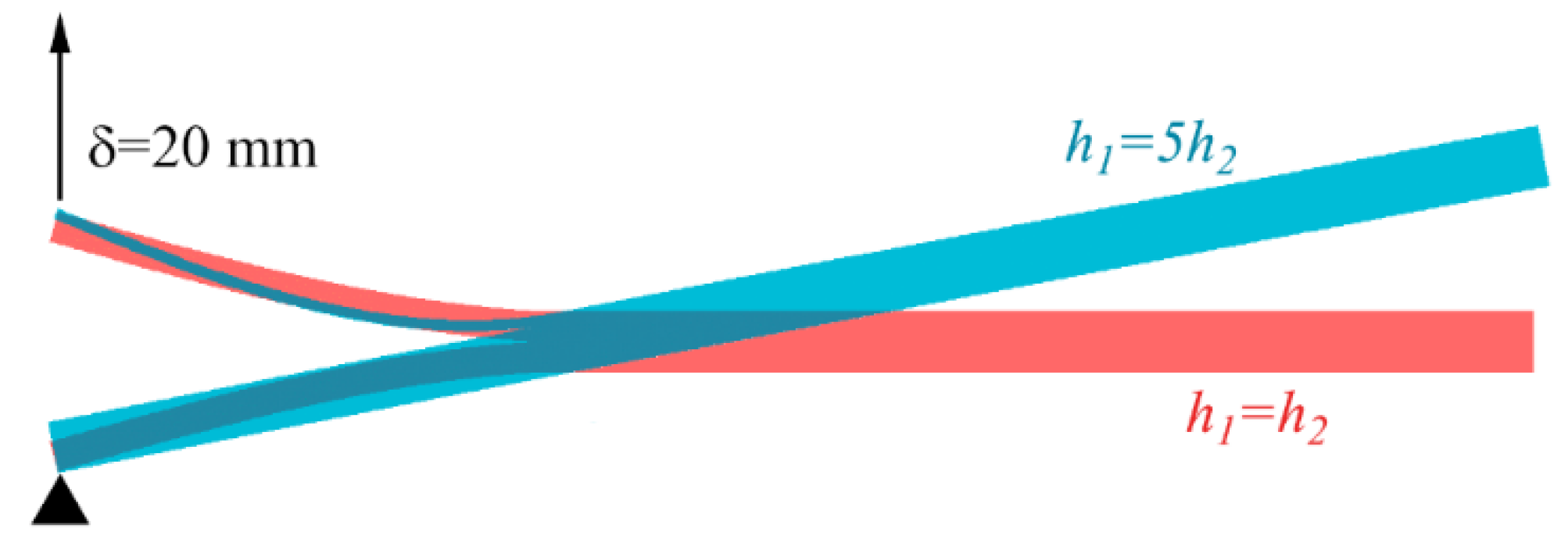
Figure 14.
Crack onset and growth in global and local coordinate systems
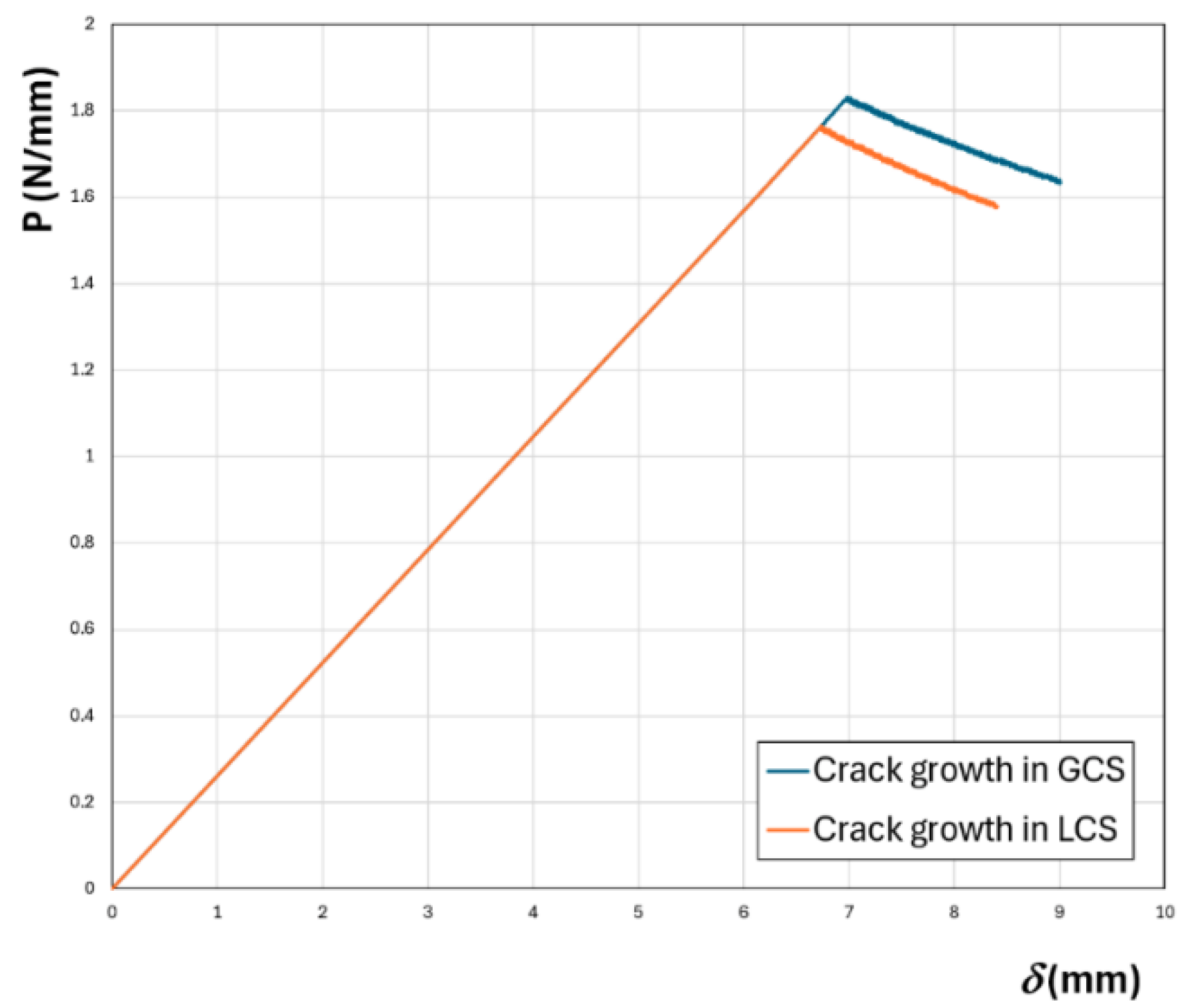

Table 1.
Mechanical properties of laminate AS4/8552.
| Property | AS4/8552 |
|---|---|
| Ex (MPa) | 144,000 |
| Ey (MPa) | 10,600 |
| Ez (MPa) | 10,600 |
| Gxy (MPa) | 5,360 |
| Gxz (MPa) | 5,360 |
| Gyz (MPa) | 3,786 |
| vxy | 0.34 |
| vxz | 0.34 |
| vyz | 0.40 |
| GIc (N/mm) | 0.250 |
| GIIc (N/mm) | 0.791 |
Table 2.
Linear and non-linear calculations. TSEM procedure.
| Solution procedure | P (N) | GI (N/mm) | GII (N/mm) | GT (=GI+GII) (N/mm) |
GT (-dU/(Bda) (N/mm) |
%GI | %GII |
|---|---|---|---|---|---|---|---|
| Linear | 2.985 | 0.288 | 0.093 | 0.382 | 0.382 | 76% | 24% |
| Non-linear | 3.008 | 0.282 | 0.102 | 0.384 | 0.385 | 74% | 26% |
Table 3.
Total energy release rate calculated by means of TSEM and analytical formulation (eq. 6)
| Calculation procedure |
GT (N/mm) TSEM (Eqs 3 and 4) |
GT (N/mm) Analytical equation (Eq. 6) |
Δ (mm) | Var. TSEM-Analytical |
|---|---|---|---|---|
| Linear | 0.382 | 0.385 | 3.04 | -0.4% |
| Non-linear | 0.384 | 0.382 | 2.12 | -0.2% |
| δ (mm) | P (N) | δ/P (mm/N) | GI (N/mm) | GII (N/mm) | GT (N/mm) | GI/GT | GII/GT |
|---|---|---|---|---|---|---|---|
| 1 | 0.664 | 1.506 | 0.014 | 0.005 | 0.019 | 75% | 25% |
| 5 | 3.347 | 1.494 | 0.348 | 0.127 | 0.476 | 73% | 27% |
| 10 | 6.802 | 1.470 | 1.332 | 0.586 | 1.919 | 69% | 31% |
| 15 | 10.404 | 1.442 | 2.854 | 1.523 | 4.376 | 65% | 35% |
| 20 | 14.254 | 1.403 | 4.825 | 3.117 | 7.942 | 61% | 39% |
| δ (mm) | P (N) | δ/P (mm/N) | GI (N/mm) | GII (N/mm) | GT (N/mm) | GI/GT | GII/GT |
|---|---|---|---|---|---|---|---|
| 1 | 0.664 | 1.506 | 0.014 | 0.005 | 0.019 | 75% | 25% |
| 5 | 3.347 | 1.494 | 0.347 | 0.127 | 0.474 | 73% | 27% |
| 10 | 6.802 | 1.470 | 1.335 | 0.587 | 1.922 | 69% | 31% |
| 15 | 10.404 | 1.442 | 2.866 | 1.528 | 4.394 | 65% | 35% |
| 20 | 14.254 | 1.403 | 4.856 | 3.135 | 7.991 | 61% | 39% |
| δ (mm) | P (N) | δ/P (mm/N) | GI (N/mm) | GII (N/mm) | GT (N/mm) | GI/GT | GII/GT |
|---|---|---|---|---|---|---|---|
| 1 | 0.664 | 1.506 | 0.014 | 0.005 | 0.019 | 76% | 24% |
| 5 | 3.347 | 1.494 | 0.363 | 0.112 | 0.474 | 76% | 24% |
| 10 | 6.802 | 1.470 | 1.486 | 0.436 | 1.922 | 77% | 23% |
| 15 | 10.404 | 1.442 | 3.431 | 0.963 | 4.394 | 78% | 22% |
| 20 | 14.254 | 1.403 | 6.297 | 1.694 | 7.991 | 79% | 21% |
Table 7.
TSEM. Change in ERR values (GI, GII and GT= GI+GII) in local and global coordinate systems. Superscript “L” denotes local coordinates and superscript “G” denotes global coordinates .
Table 7.
TSEM. Change in ERR values (GI, GII and GT= GI+GII) in local and global coordinate systems. Superscript “L” denotes local coordinates and superscript “G” denotes global coordinates .
| δ (mm) | Rotated angle (rad.) | Crack tip node x-displacement (mm) | |||
|---|---|---|---|---|---|
| 1 | -1% | 2% | 0% | 0.0035 | -0.022 |
| 5 | -4% | 14% | 0% | 0.0292 | -0.196 |
| 10 | -10% | 35% | 0% | 0.0713 | -0.571 |
| 15 | -16% | 59% | 0% | 0.1172 | -1.116 |
| 20 | -23% | 85% | 0% | 0.1647 | -1.836 |
Table 8.
ERR partition values of several samples with different h2/h1 and E2/E1 rates. GCS: Global Coordinate System. LCS: Local Coordinate System. δ=10 mm. a0=50 mm.
Table 8.
ERR partition values of several samples with different h2/h1 and E2/E1 rates. GCS: Global Coordinate System. LCS: Local Coordinate System. δ=10 mm. a0=50 mm.
| E1 (MPa) | E2/E1 | h2/h1 | GCS %GI |
GCS%GII | LCS %GI | LCS %GII | Rotated angle (rad.) | |
|---|---|---|---|---|---|---|---|---|
| 144000 | 1 | 1.000 | 1.000 | 100% | 0% | 100% | 0% | 0 |
| 144000 | 1 | 0.714 | 0.510 | 95% | 5% | 97% | 3% | 0.0323 |
| 144000 | 1 | 0.500 | 0.250 | 84% | 16% | 88% | 12% | 0.0563 |
| 144000 | 1 | 0.333 | 0.111 | 72% | 28% | 79% | 21% | 0.0697 |
| 144000 | 1 | 0.200 | 0.040 | 62% | 38% | 71% | 29% | 0.0751 |
| 144000 | 0.25 | 0.200 | 0.010 | 43% | 57% | 52% | 48% | 0.0812 |
| 144000 | 0.125 | 0.200 | 0.005 | 39% | 61% | 48% | 52% | 0.0822 |
Table 9.
Crack onset critical values in global (GCS) and local (LCS) coordinates
| δc (mm) | Pc (N/mm) | |
|---|---|---|
| GCS | 6.99 | 1.832 |
| LCS | 6.74 | 1.765 |
Disclaimer/Publisher’s Note: The statements, opinions and data contained in all publications are solely those of the individual author(s) and contributor(s) and not of MDPI and/or the editor(s). MDPI and/or the editor(s) disclaim responsibility for any injury to people or property resulting from any ideas, methods, instructions or products referred to in the content. |
© 2025 by the authors. Licensee MDPI, Basel, Switzerland. This article is an open access article distributed under the terms and conditions of the Creative Commons Attribution (CC BY) license (http://creativecommons.org/licenses/by/4.0/).
Copyright: This open access article is published under a Creative Commons CC BY 4.0 license, which permit the free download, distribution, and reuse, provided that the author and preprint are cited in any reuse.


