Submitted:
21 April 2025
Posted:
22 April 2025
You are already at the latest version
Abstract
The nature of solar activity (SA) cycles close to orbital period of Jupiter and role of galactic factors in evolution of biosphere are still open. In order to solve first problem, it was proposed to take into account interaction between the magnetic dipoles of planets and Sun along with tidal effects. Correlations with a period close to one quarter of Solar System (SS) revolution time around the Galactic center (~63 Myr) were revealed in changes in geochronologies of terrestrial paleomagnetism and global temperature of Phanerozoic. Their probable cause may be a change in tidal and magnetic effects of stars when SS crosses spiral arms of Galaxy. The key role of Jupiter in generating SS magnetic field is evidenced by effect of Shoemaker-Levy comet falling on it in 1994. Since 1995, the interplanetary magnetic field has halved and changes in parameters of 23rd and 24th SA cycles have affected chronologies of geophysics, thermal physics of hydrosphere and biosphere. It was suggested that electron neutrino decays in Sun into chiral quanta, which are embedded in magnetic field lines and metabolized in biosystems by condensation on coherent ensembles of protons or magnetic moments of metals in enzymes and liquid media. In this way, dependence of metabolism and cognitive functions of human brain on balance of trace elements and geomagnetic storms is realized. The globalization of introduction of digital technologies into the human ecosystem has stalled natural mechanisms of development of child's brain and creativity in adult homo sapiens. Human consumer parasitism on biosphere has reached a planetary level and anthropogenic factor has aggravated effects of abiogenic factors of regular Sixth Global Extinction.
Keywords:
Magnetic field
; Sun
; Jupiter
; Earth
; neutrino
; water
; biosphere
1. Introduction
The impact of comet Shoemaker-Levy 9 (SL9) on Jupiter (hereinafter Fall-SL9) occurred in July 1994 [Impact events]. Before Fall-SL9, back in 1992, the comet broke up into 21 fragments at the closest point to Jupiter on its elliptical trajectory. Despite the unprecedented nature of this event in the era of space observations, it has not received due attention in modern astronomy of the Sun and the Solar System (SS). Meanwhile, Jupiter has a powerful magnetic field and the time of its revolution around the Sun (~11 years) correlates with the periodicity of Solar Activity (SA). Jupiter, like the electron and proton in the hydrogen atom [Kholmanskiy, 2017], can modulate the dynamics of the interplanetary magnetic field (IMF) and SA
through its interaction with the magnetic dipole of the Sun. It was suggested that the disturbance of Jupiter’s magnetism by Fall-SL9 manifested itself after 1995 by violations of the SA parameters and failures in the chronologies of geophysical and meteorological indicators of the biosphere associated with geomagnetism and thermodynamics of the hydrosphere. To verify this hypothesis and clarify the probable mechanism of the influence of Jupiter’s magnetic field on the Sun and biosphere, the chronologies of geophysical and meteorological indicators with a reliable break in ~1995 were analyzed. Using the known data on the physics of the Sun and Jupiter, the induction mechanism was used to explain the transmission of the disturbance of Jupiter’s magnetic field by Fall-SL9 to the SA. The possibility of the solar neutrino’s participation as a chiral factor of magnetic nature in anthropogenesis and regulation of hydrosphere’s thermodynamics was discussed.
2. Materials and Methods
2.1. Empirical Materials
The work conducted a comparative analysis of known
SA monitoring data, geophysical and meteorological indicators for the period
from ~1970-2020. In the reviews [Blunden, 2020; 2023; Johnson, 2023; Lindsey,
2023; Schuckmann, 2023], chronologies of land, ocean and atmospheric indicators
with linear intervals of 15-20 years before and after ~1995 were selected. For
these chronologies, the rates of change of indicators (k) were determined with
~10% accuracy using the kt approximation, where t is years. By comparing k for
anomalies of related indicators, information was obtained on the factors involved
in triggering changes in the state of the geospheres in 1995. The k values are
shown in the boxes on the graphs, their dimension is “magnitude/year”. When
analyzing the changes in k chronologies of thermophysical indicators, the
following data were taken into account. About ~90% of heat on Earth is
contained in ocean water, of which ~60% is in upper layer up to 700 m and 30%
is in the water layer from 700 m to the bottom [Rhein, 2013; Lindsey, 2023].
The remaining ~10% of Earth’s heat is summarized by share of land ~5%,
cryosphere ~4% and atmosphere ~2% [Schuckmann, 2023].
To clarify mechanism of thermal rearrangements of
condensed media (water, quartz) and atmosphere, effective activation energies
(EA) of the key stages of molecular dynamics were determined. Analysis of known
temperature dependences (TDs) was carried out using the method [Kholmanskiy,
2019c; 2021]. Empirical TDs were approximated by exponential exp(EA/RT).
The EA values were given in kJ/mol and compared with known data for
water and aqueous solutions. To substantiate the mechanisms of the influence of
geomagnetism on the cognitive functions of brain, cooperative properties of
hydrogen bond network in physiological fluids and high magnetic susceptibility
of metal isotopes, which play an important role in trophic and signaling system
of brain, were taken into account. The graphical data were digitized using
Adobe Photoshop, and chronology approximations were obtained using Excel.
2.2. Hypotheses and Relationships
In practice, mathematical formalization of magnetic
field manifestations successfully does without any ideas about the physical
nature of its carrier. Meanwhile, the possibility of decay, sterility, aroma,
and elusiveness of solar neutrino [Athar, 2022] allow its use in the
mathematical formalization of magnetic Faraday tubes [Maxwell, 1954; Solanki,
2013] and a chiral quantum of energy with biogenicity [Kholmanskiy, 2016; 2018;
2024a]. This hypothesis is based on the decay of electron neutrino (νe)
of the p-p cycle in the Sun’s core into energy quanta (ℵ-forms), the number of which is limited by the Avogadro
number (N ~ 6 1023) [Kholmanskiy, 2003; 2011a]. Conditionally
sterile ℵ-forms preserve
the helicity of neutrinos and model the energy forms of ether (ν/g-vortices),
combining rotational and translational motion according to the law of
electromagnetic induction [Kholmanskiy, 2006]. Note that the axiomatics of ν/g-vortices
is suitable for the formalization of hypothetical subelectronic fractal
matter [Puetz, 2015]. When N ν/g-vortices or ℵ-like
forms merge in compliance with the symmetry rules (N-condensation), quanta of
fields and elements (shell and orbitals) of particle and nuclear structures are
formed [Kholmanskiy, 2017; 2019]. The kinematics and dynamics of ℵ-forms are limited by the
angular velocity of the g-vortex (~1023 s–1) and the momentum
transfer velocity along the g-grid of ether, equal to C(N)1\2 ~ 2.3
1020 m/s, (C is speed of light in a vacuum) [Kholmanskiy, 2003;
2011a; 2016]. From ℵ-forms,
as from monopoles, tubes of magnetic field lines can be formed [Solanki, 2013;
Jeong, 2020]. In the radiative zone of the Sun, chiral neutrino-photon forms (ℵγ) can be formed
during the interaction of ℵ-forms
with γ [Giunti, 2015]. Similar interactions can probably occur in convective
zone of Sun, as indicated by modulation of solar radiation by magnetic activity
of photosphere [Domingo, 2009; Krivova, 2021]. At the same time, the chirality
sign ℵγ can
change when the magnetic dipole of Sun is reversed in Hale cycle. The parity of
participation in energy of Sun of photons (γ) and νe can be realized
by the chiral synergism of γ and ℵγ
at all stages of evolution of biosphere.
Solar physics, geophysics and unique position of
Earth in SS determined the stable coverage of its surface by hydrosphere by
~70% [Sorokhtin, 2010]. The global temperature (TG) at bottom of ocean could be
maintained in range of ~0°-4° even during glaciation periods and up to ~40° at
other times. At such T, proteins in free water and in physiological fluids
retained their nativeness and ability to complex with participation of hydrogen
bonds of water (HBs) and other chemical elements. [Kholmanskiy, 2023; 2019;
Globus, 2020]. N-condensation of ℵ-forms
and ℵγ in
hydrosphere and physiological fluids on chiral centers or nuclear spins of
cooperative biosystems could catalyze biochemical reactions. The lithosphere
consists of ~70% silica, containing equal amounts of left and right quartz
crystals [Kizel, 1985] and therefore can propagate incident ℵγ fluxes as a
waveguide. The dependences of the elastic properties and thermal conductivity
of the lithosphere on the density of ℵγ
fluxes and geography can manifest themselves in changes in ocean thermal
physics and crustal seismic activity. On night side of Earth, the actions of ℵ-forms and ℵγ can catalyze dark
biochemistry of circadian rhythm [Michel, 2019; Kholmanskiy, 2019; 2023].
The biogenicity of geomagnetic field is manifested
in magnetoreception of birds. The effect of magnetic field of Helmholtz coils
in biosystems depends on chirality of reagents and signs of magnetic moments of
elements participating in reactions [Zadeh-Haghighi, 2022]. These results are
consistent with the assumption of the neutrino nature of magnetic field
carriers. When modeling the hypothetical structures of Sun, Jupiter and Earth,
we relied on bootstrap principle and scaling law [Glattfelder, 2019]. They are
based on dialectical law of similarity and quantum rules of
self-assembly-condensation of ν/g-vortices into chiral elements of particles
and nuclei [Kholmanskiy, 2008; 2011a]. The rules minimize the effect of ν/g-vortices,
particles and molecules of the Planck constant (h) and limit their number N,
which is necessary for condensate to acquire a new quality. The
self-organization of supporting elements of hierarchy of Universe proceeded in
compliance with these rules, which is illustrated by proximity to N in order of
magnitude of ratios of radii of Sun (~7 1010 cm) and helium nucleus
(~1.2 10-13 cm), hydrogen atom ~5 10-9 cm and orbit of Jupiter ~8 1013
cm, as well as proximity of ratio of masses of Sun (~2 1033 g) and
Jupiter (~2 1030 g) to ratio of masses of proton (~1.7 10-24
g) and electron (~9.1 10-28 g). During N-condensation of water
molecules (1 mol), 1 cm3 of liquid water weighing 1 gram is formed
[Kholmanskiy, 2003; 2019]. The state of matter and mechanism of rotation of
stellar nuclei are modeled by physics of neutron stars [Lattimer, 2004]. The
inner cores of Earth-type planets could have formed from iron atoms by their
N-condensation into axially symmetric structures of hexagonal clusters [Tateno,
2010; Dewaele, 2023].
3. Results and Discussions
3.1. Jupiter and Heliophysics
Due to gravity and magnetism of Sun and planets,
Solar System (SS) is in dynamic equilibrium and the motion of planets in it
obeys, in first approximation, Kepler’s third law:
R3 ~ Y2,
R is distance between centers of mass of planet and
Sun; Y is orbital rotation period of planet. At a qualitative level, the tidal
effects between planets and Sun will directly depend on their masses and
inversely proportional to R3. The energy of interaction of the
magnetic dipoles of planets and Sun (μS) obeys the same dependence
on distance. For example, the magnetic effect (Jμ) of Jupiter’s dipole
(μJ) is expressed by the formula:
Jm~ mS mJ /R3
Taking values of tidal and magnetic effects of
Earth as a unit, we estimated their ratios (Pμ/Pt) for SS
planets (Table 1). The orbital period of
Jupiter (YJ = 11.86 years) is comparable with the average duration
of Schwabe cycle (YS = 10.8±0.5 years) [Manda, 2020; Hathaway,
2010], which links the magnetic activity of the Sun with the number of sunspots
(W, Figure 1A). Two adjacent Schwabe
cycles are combined into one Hale magnetic cycle (~22 years), during which a
reversal of magnetic fields of northern (N) and southern (S) hemispheres in the
Sun occurs and a change in sign of its global magnetic field occurs (Figure 2, Figure 3) [Hathaway, 2010; Strugarek, 2017; Okhlopkov, 2020; Pipin, 2006]. The
difference between YJ and YS varies in range from 5% to
~13%, and there are no long-term correlations of Schwabe cycles with perihelion
and aphelion of J orbit (Figure 2B). Figure 1A shows Schwabe cycle averaged over
amplitude and period and an example of approximating distribution of magnetic
elements on solar surface by arbitrary third-degree polynomials [Hathaway,
2010; Krivova, 2021].
According to Formulas (1) and (2), a physically adequate approximation of Schwabe cycle is C.t2 function (Figure 1B), which allows one to distinguish two linear intervals on ascending and descending branches, as well as a plateau lasting ~2 years at cycle maximum. This partitioning of Schwabe cycle illustrates complex dependence of sunspot generation mechanism on tidal (Pt) and magnetic (Pμ) effects of the SS planets [Hung, 2007; Okhlopkov, 2020; Krivova, 2021]. Computer programs for calculating dynamics of ephemerides of SS planets and combinatorics of syzygies in Jupiter-Venus-Earth-Saturn configuration make it possible to obtain approximations of long-term chronologies of Schwabe cycle close to observed ones [Nandy, 2021; Stefani, 2024; Scafetta, 2023]. However, the lack of adequate formatting of magnetic effects of planets with a high Pμ/Pt ≥1 value (Table 1) in these models leaves open main question of heliophysics—the role of solar magnetic field in genesis and biophysics of ℵ-forms and ℵγ [Kholmanskiy, 2011; 2019; Nataf, 2023; Weisshaar, 2023; Obridko, 2020; 2024].
The dominance of contribution of Jupiter magnetic effect (Jμ) to solar physics disturbances (Table 1) will be manifested in Schwabe cycles with a high level of correlation of W chronology with J orbital parameters. This condition is well satisfied for Schwabe cycles 22, 23, and 24 (Figure 2B). The plateau regions in graphs of these cycles are located between perihelion and aphelion within errors of best approximations given in [Scafetta, 2023]. In addition, centers of these plateaus and periods of transformation of magnetic dipoles of solar hemispheres into a quadrupole (QS) correlate well with time of Jupiter’s crossing of solar equatorial plane (SE). Synchronization of changes in Schwabe cycle with motion of Jupiter is determined by level of resonance of Jμ with sunspot generation mechanism, which depends on following factors. For Jupiter and Saturn, due to difference in RP, the tidal and magnetic effects at perihelion are ~1.4 times greater than at aphelion. The orbital inclination of all planets with Pμ/Pt ≥1 to solar equator is ~6°, so at perihelion and aphelion, these planets will be ~0.1Rorbit below and above SE, respectively. The magnetic effect of planets with Pμ/Pt ≥1 at SE crossing will depend on axial asymmetry of their magnetic fields and direction of global dipoles. These differences may affect W chronologies and flare rates [Li, 2009; Badalyan, 2011; Nandy, 2012; Javaraiah, 2020; 2021].
3.2. Magnetism of Sun and Jupiter
Models of axisymmetric structures of Sun and Jupiter (Figure 3, Figure 4) are similar to structures of nuclei and particles consisting of spherical shells and chiral toroidal orbitals (inner and outer) [Kholmanskiy, 2017]. Semi-empirical quantum mechanical calculation of models of structures of nuclei and particles yielded parameters close to measured ones [Kholmanskiy, 2017; 2019]. The circulations of meridional magnetic field lines through polar windows in shells of Sun and Jupiter correspond to their magnetospheres and hemispheric fields. Flares and torches are activated in regions of polar windows of convective zone of Sun [Sivaraman, 2010]. The solar envelope models a thin-layer tachocline, and toroidal orbitals are elements of rotational structure of Sun and Jupiter, including chiral dynamo ring currents in N and S hemispheres (Figure 3) [Kholmanskiy, 2007; 2011a; Charbonneau, 1999; Strugarek, 2023; Zhukova, 2024]. The helicity of global magnetic field and convective zone fields in solar hemispheres will depend on the chirality signs of ring current fields internal and external to tachocline [Yang, 2012; Maurya, 2020].
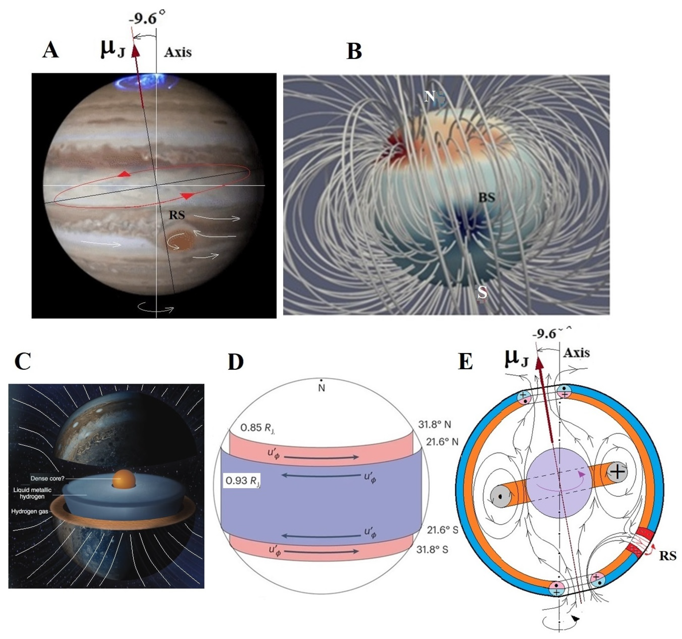
The right and left chirality of ring currents and fields of northern and southern hemispheres (Figure 3D) are consistent with symmetry of global solar magnetic field (Figure 3A). The solar core and radiative zone rotate in solid body approximation, with core rotating faster than radiative zone [Fossat, 2017; Kholmanskiy, 2017]. Large-scale ring currents in vicinity of solar tachocline (Figure 3C) and in near-surface layers of Jupiter (Figure 4C, Figure 4D), like alternating windings of inductive coils, can generate magnetic dipoles and quadrupoles (Figure 3D) [Beaudoin, 2012; Zhukova, 2024]. Substituting the values of ratio μS/μJ ~ 230 (Table 1), the radius of tachocline (~0.7RS [Charbonneau, 1999]) and current sheets of Jupiter (~0.9RJ, Figure 4D) [Hori, 2023] into formula for ring current dipole:
then we obtain the ratio of current values IS/IJ ~ 4. It corresponds to conventional four current rings of Sun (Figure 3D) [Kholmanskiy, 2007] and conventionally one current ring J (Figure 4E). According to formula (3), the dipoles of the northern (μN) and southern (μS) hemispheres of Sun will be proportional to ring currents and orthogonal to their planes. The physics of Jμ effect can be based on inductive interaction between magnetic dipoles according to formula (2) and resonant transfer of energy between ring currents [Tesla; Singh, 2012].
m = πIr2
Figure 3.
A—Latitudinal distribution of solar wind (proton) velocity. Image of Sun in optical and soft X-ray ranges. White arrows—direction of magnetic field lines. B—blue dots—sunspots for 6 months of 23rd solar cycle. Lines mark boundaries of oscillations of planes of current rings, and angles (θn, θs) mark the deviations from axis of dipoles of northern and southern hemispheres (μN, μS). C—the solar core (red), convective (white) and radiant zone (yellow), ring currents in the hemispheres (black and red circles), radial currents (green arrows), poloidal magnetic fields (red and blue areas above tachocline). D—convective zone (1), tachocline shell (2), radiant zone (3); ring current tori: right (4R), (6R) in N hemisphere; left (5L), (7L) in S hemisphere; sunspots (8). Figures adapted: C from [Nandy, 2021], D from [Kholmanskiy, 2007; 2017; Gavelya, 2018].
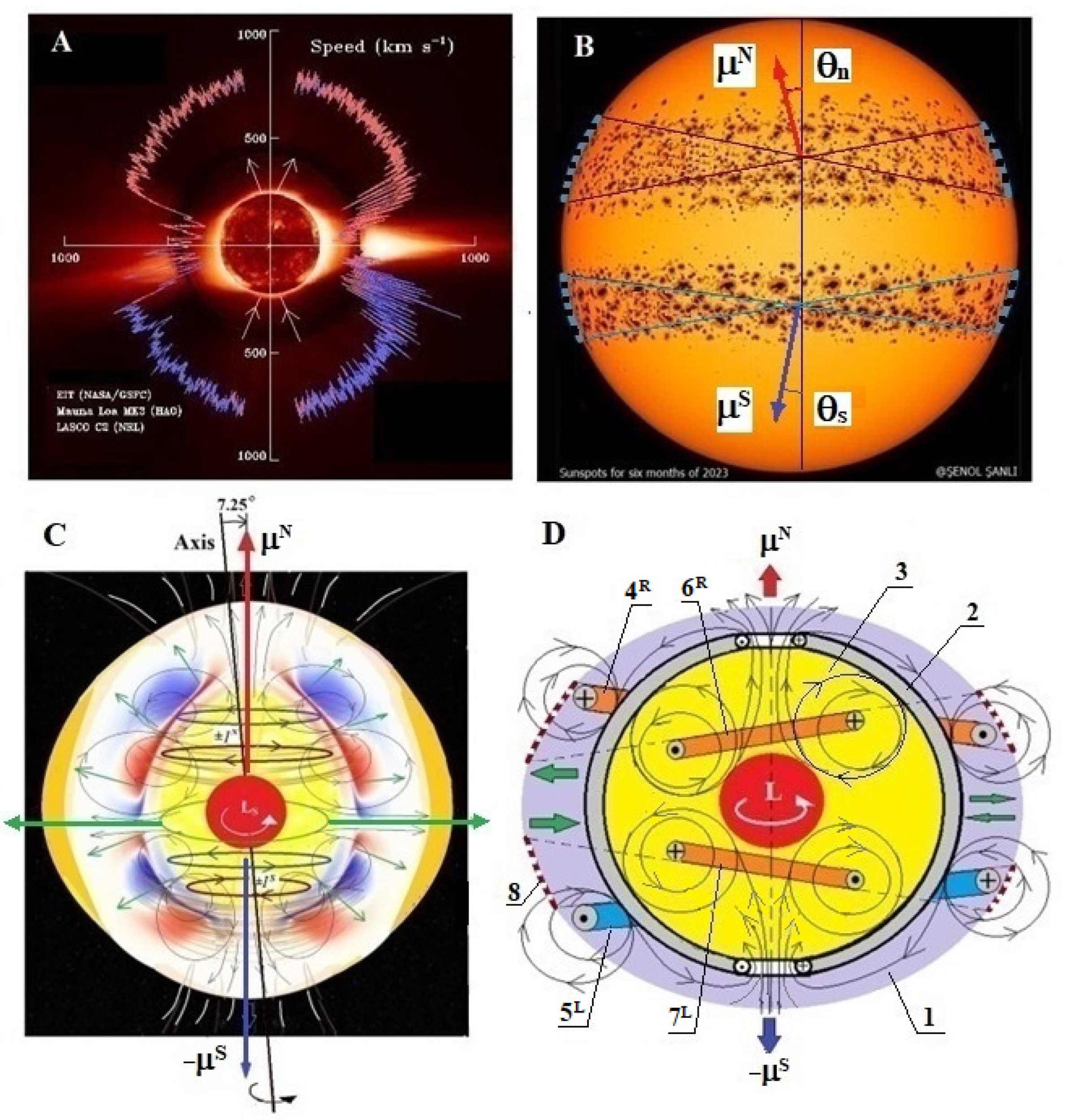
Figure 4.
A—photo of Jupiter, μJ—magnetic dipole of Jupiter’s ring current (red circle), white arrows—atmospheric flows in vicinity of Great Red Spot (RS), pink arrow and dotted curve—trajectory of falls of fragments of comet Shoemaker-Levy (SL9). The aurora borealis circle is located above the vortex hole in the shell shown in E. B—view from the equator of magnetic field lines, BS—entrance of lines into the Great Blue Spot. C—An artist’s rendition of Jupiter. The core is possibly molten and surrounded by liquid metallic (LMH) and gaseous hydrogen. Magnetic field lines are due to dynamo effect of LMH. D—diagram of Jupiter’s surface current sheets (blue-red). E—lilac core of Jupiter, right current ring (orange) and left-right currents in two layers of the shell (blue-red); magnetic field fluxes of ring and turbulent flow of incoming sheath currents induce left-handed ring currents (red stripes) of Great Red Spot (RS) in it. Figures B, C, D and E are adapted from [Moore, 2018], [Silvera, 2021], [Hori, 2023], and [Kholmanskiy, 2017], respectively.
Under influence of Jm, antiphase displacements of planes of currents 4R and 5L (Figure 3D) will generate turbulence in differential rotation of convective zone and meridional motion of plasma [Nandy, 2012; Beaudoin, 2012; Zhukova, 2024]. Coriolis forces initiate formation of poloidal fields and twisting of radial currents into spirals [Gavelya, 2018; Hanasoge, 2022]. Bundles of magnetic field tubes strung on current spirals [Solanki, 2013] will appear on surface of photosphere as spots at latitudes of ~10-25° in both hemispheres [Klevs, 2023; Gnevyshev, 1977]. The effect of Jm on the 6R and 7L ring currents in the radiative zone (Figure 3D), weakened by tachocline, can cause synchronous with W changes in facular activity at high latitudes of photosphere [Sivaraman, 2010; Takalo, 2023]. The axial asymmetry of Jm (Figure 4B) [Moore, 2018] will cause differences in distribution of spots and magnetic fluxes in active regions of N and S hemispheres of Sun (Figs. 3B, 3D) [Zhukova, 2023; 2024; Zwaan, 1978; 2010; Nandy, 2021; Hotta, 2021].
A dependence of correspondence between changes in W and magnetic flux (Flux) in cycles 22, 23, and 24 on position of Jupiter relative to SE plane is observed (Figure 2, Figure 5). In cycle 23, during period of maximum SA between perihelion and point of Jupiter’s intersection with SE, changes in W and Flux roughly correlate in regular and irregular active regions (ARs) in both hemispheres of Sun. In cycle 24, Jupiter’s intersection with SE correlates with place where Schwabe cycle is divided into two halves by Gnevshev gap [Gnevyshev, 1977; Takalo, 2023]. For irregular ARs in cycle 24, correlation between changes in W and Flux is preserved, but a sharp increase in Flux is observed in the S hemisphere after Jupiter’s intersection with SE (Figure 5). In regular ARs, the correlation level between W and Flux decreases sharply before and after SE crossing, and an asymmetry between Flux changes arises: in N hemisphere, Flux is higher before SE crossing and decreases after, and vice versa in N hemisphere. Such changes in regular ARs of cycle 24 can be associated with dependence of Jm effect on strength of resonant interactions between dipoles of N and S hemispheres of Sun and Jupiter, which changes when Jupiter crosses SE and after fall of comet SL9 on it (Figure 2B). In this context, the nature of regular ARs can be associated with averaged effects of tidal and magnetic effects of all SS planets on Sun. Increased dominance of Jμ at perihelion and aphelion, as well as when Jupiter crosses the SE, can lead to the appearance of additional disturbances of the solar magnetic field, generating irregular ARs.
The Gnevyshev gap divides even Schwabe cycles into two SA maxima, which correspond to different events spaced 2-3 years apart in time, and at latitudes of 25° and 10° in both hemispheres of Sun [Gnevyshev, 1977; Takalo, 2023]. In the case of cycle 24, time shift of SA maxima is synchronized with Jupiter crossing SE and reversal of mS through intermediate configuration of quadrupole (QS, Figure 2B). The rates of reversible changes in inclinations of current planes (4R, 5L) during reversal period (~2.5 years) will be of the same order of magnitude as meridional drift velocity of sunspots, equal to 20 m/s [Hanasoge, 2022]. The process of polarity reversal can be modeled by following diagram of sequence of changes in convective zone of inclinations of planes of currents 4R, 5L and the precessions (θn, θs) of the dipoles mN and mS:
- a)
- at beginning: mN sinθn—mS sinθs ~ 0 и mS = mN cosθn—mS cosθs > 0;
- b)
- isthmus: mN cosθn—mS cos φs ~ 0 и QS = mN sinθn—mS sinθs > 0;
- c)
- at end: mN sinθn—mS sinθs ~ 0 и mS = mN cosθn—mS cos θs ~ 0.
At stages a) and c), at points of stopping and reversal of current plane displacement, maximum excitation of convective turbulence occurs, which leads to an increase in W. Thus, the mechanisms of W generation in Schwabe cycle and μS polarity reversal in the Hale cycle integrate all factors of dependence of Jμ on features of Jupiter’s orbit and interaction of μJ with μS. The influence of Jμ on helicity of solar magnetic field can cause synchronization of variations in interplanetary magnetic field with changes in chirality and intensity of fluxes of ℵ-forms ℵγ. Note that specificity of magnetic effects of planets on Sun is not characteristic of tidal effects, and universality and range of Jμ are illustrated by electromagnetic connections of Jupiter with its satellite Io [Schneider, 2007] and “hot Jupiter” with its star [Cauley, 2019].
3.3. Comet Shoemaker-Levy Fall on Jupiter
The comet fragments crashed into southern hemisphere J one after another at a latitude of ~44°S with an interval of ~7 hours, with the rotation time of J around its axis being ~10 hours. With collision temperature reaching ~24000K, a necklace of plasma clots and trails of ionized elements was formed at a latitude of ~44°S. From the places where large pieces of comet fell, J waves diverged upward through atmosphere at a speed of ~450 m/s [Ingersoll, 1995]. They could correspond to deformation waves in dense conductive layers of S-hemisphere (Figure 4D). During year of relaxation after Fall-SL9, the waves could reach current sheets in N-hemisphere and induce ring currents in them, magnetic fields of which transformed axial magnetic field of N-hemisphere into a non-dipole one (Figure 4B). When magnetic field flows entering S-hemisphere and generated by current ring merge, a magnetic flux tube can be formed [Solanki, 2013], which generates ring currents in layers of shell and atmospheric vortex of Great Red Spot (RS, Figure 4E). The N/S asymmetry of Jupiter dipole and configuration of global magnetic field persisted until 2016 [Moore, 2018]. The relaxation process of Jupiter magnetic field was reflected in changes in helicity of total magnetic flux of northern and southern hemispheres of Sun in 23rd SA cycle. At beginning of cycle (1996-1997), the helicity was positive in N hemisphere, on plateau of Schwabe cycle (2000-2003), the sign fluctuated and became negative in S hemisphere in 2003-2004 [Yang, 2012; Zhang H, 2013]. This restructuring in solar electrodynamics led to a twofold decrease in solar magnetic field by end of 23rd cycle and a significant N/S asymmetry in generation of polar magnetic fields after 1995 [Ishkov, 2018]. These changes in physics of Sun in cycles 23 and 24 caused a decrease in the interplanetary magnetic field by 2/3 and a decline in geoeffectiveness of all SA manifestations [Toma, 2009; Sheeley, 2010; Zerbo, 2013; Hady, 2013; Vidotto, 2018; Javaraiah, 2021; Zhang J, 2021].
3.4. Earth Echo of Fall of Comet SL9
3.4.1. Hydrosphere and Atmosphere
Changes magnetism of Sun and SS after falling comet SL9 on Jupiter should correspond to changes in intensity and chirality of ℵ-form and ℵγ fluxes. It is hoped that analysis of chronologies of geomagnetism, meteorological indicators of climate and state of various biosystems will allow us to differentiate mechanisms of action of sunlight (γ) and chiral factor (ℵγ) on the biosphere. For this, chronologies with a break in range of 1970-2020 are suitable, which are divided in region of 1995±0.5 years into two fairly linear dependencies with different k. Numerous observations show an increase in rate of heat accumulation on Earth after 2000, but causes of this global phenomenon have not yet been established [Schuckmann, 2023]. Note that anomaly of 2000 in these observations may be due to a 5-year shift by mechanism of retransmission of Fall-SL9 effect by Sun to Earth’s physics. However, even in such chronologies of the hydrosphere and atmosphere thermal physics indicators, a break can be detected in 1995.
The positive (F9) and negative (1/F9) effects of Fall-SL9 will manifest themselves, respectively, as an increase and decrease in k after 1995:
The F9 values for rates of thermal energy accumulation by glaciers, ocean, and atmosphere are ~1.7-5.0, ~3, and ~2, respectively (Figure 6B, Figure 7). After 1995, contributions to annual change in global heat from ocean, ice, and air are 94%, 4%, and 2%, respectively. With such a distribution of heat content shares, ocean will act as a thermostat and stabilize TG, which is confirmed by low F9 values for atmosphere ~1.5 (Figure 8A), air over ocean ~1.6, and land ~1.1 (Figure 9A). The same is evidenced by proximity of F9 for Arctic sea ice melting rate ~3.4 (Figure 8B) to F9 value for ocean layers up to 2000 m (Figure 6).
A sharp jump in heat content in upper ocean layer after 1995 initiated circulation of heat flows between equatorial and polar zones of ocean [Johnson, 2024]. Intense water evaporation led to an increase in water density in low layers of atmosphere and its heating (Figure 8A, Figure 9A). The response of ocean thermal physics to Fall-SL9 can be associated with occurrence in 1997–1998 of most powerful El Nino phenomenon in entire history of observations, which led to large-scale droughts, floods, and other natural disasters around world [El Nino]. The rate of ocean heating in layer up to 700 m is determined mainly by the intensity of γ flux, which in SA cycle 23 oscillates with a period of ~2 years with an average k value 1.4 times greater than in SA cycle 24 (Figure 6A). The solar luminosity rhythm is generally modulated by mechanism of magnetic field generation on solar surface [Zwaan, 1978; Solanki, 2013; Shapiro, 2017; Domingo, 2009; Krivova, 2021]. This modulation after Fall-SL9 could have been superimposed by periodicity of relaxation process of Jupiter’s magnetic field, which manifested itself in two-year waves in chronology of 23rd SA cycle and synchronous changes in thermal physics of ocean.
3.4.2. Lithosphere and Geomagnetism
Due to close magneto-gravitational connections, the Sun, Jupiter and Earth can be represented as a single physical system (SJE), which experiences periodic magnetic-tidal disturbances from stars of Galaxy and rest of SS planets, as well as from random collisions of J and E with comets and asteroids. In accordance with the principles of certainty, the structure of SJE can be likened to an atom, and the structures of Sun, J and E (Figure 3, Figure 4, Figure 10) can be represented as models of nuclei and elementary particles [Kholmanskiy, 2017; 2019]. Despite the significant difference in chemical composition and temperature in the nuclei of Sun, J and E, principle of magnetodynamo operation is the same for them. It is based on transfer of heat, mass and torque from inner core to the liquid outer core, in which ring currents are excited and a global magnetic dipole is generated (Figures 3E, 4D, 10A).
Estimates of heat flow from core, which determines the activity of geodynamo, differ by at least a factor of 2, and mechanism of thermal conductivity of lower mantle is still unknown [Nimmo, 2015]. Accordingly, for Earth, as well as for Jupiter, question of mechanism of generation of their magnetic fields due to energy of inner core remains open. Moreover, if for hydrogen nature of Jupiter some analogy with energy of Sun’s core is possible, then for Earth there is not even a consensus on structure and time of origin of its iron core [Biggin, 2015; Bono, 2019: Landeau, 2022].
It can be assumed that on Earth, cosmic versatility of hydrogen was realized through unique physicochemical properties of liquid water in hydrosphere and biosystems, as well as hydroxide OH- and hydrides in inorganic complexes of substance of core, mantle and lithosphere. The lability of proton spin and dynamics of hydrogen bonds in biosystems could contribute to synergism of γ and ℵγ in evolution on Earth and implementation of magnetic holism in SJE system. In addition to main geodynamo, convective electrochemical flows between outer core and mantle also participate in Earth’s magnetism [Nimmo, 2015]. These flows correspond to multipole magnetic fields on Earth’s surface, which disturb global field and can participate in its polarity reversal [Buffett, 2007; Pétrélis, 2009; Schaeffer, 2017; Davies, 2020; Butler, 2021; Landeau, 2022]. The configurations of such a field are illustrated by South Atlantic Magnetic Anomaly (SAA) (Figure 11) [Pavón-Carrasco, 2016].
The dynamics of N/S asymmetry of solar polar fields (Figure 5) after Fall-SL9 correlates with a sharp difference in drift velocity of geomagnetic poles. For N pole, it increases abruptly after 1995 to F9~6, but for the S pole it remains almost constant in the interval of 1970-2020 (Figure 12C). The dynamics of poles is accompanied by a synchronous decrease after 1995 in dipole-axial magnetic field and energy with 1/F9 equal to 1.5-2 (Figs. 12A, 12B; Figure 13A). At the same time, k for energy and radial component of non-dipole field SAA remains almost unchanged after 1995 (Figs. 13A, 13C). The distribution features of magnetic anomalies on Earth’s surface could have played role of targets for comets and asteroids with their own magnetic or dipole moment. Such a target for fall of asteroid 65 Ma was point (1) north of South Atlantic Magnetic Anomaly (SAA) and point (2) in center of Siberian Magnetic Anomaly for fall of Tunguska meteorite in 1908 (Figure 12).
At end of Archean, after the formation of global lithosphere ~2.7 Ga [Arndt, 2013], the evolution of the biosphere followed long-term rhythms of Sun and SS physics with cycles from ~0.1 Myr to ~1 Gyr [Zhang X, 2017]. The cyclicity of climate geochronology with a period of ~0.4 Myr according to Milankovitch is associated with rhythm of magnetic-tidal effect of Jupiter and Venus on the Earth’s insolation [Laskar, 2011; Wilson, 2013; Kent, 2018]. Changes in the geomagnetic field qualitatively correlate with peaks of ~0.4 Myr cycle [Landeau, 2022]. A change in polarity of the ~0.8 Ma field could have initiated a mutation in hominid genome, resulting in emergence of FOXP2 speech gene [Enard, 2002] and contributed to reproduction of marine biota, as evidenced by a sharp jump in ~0.8 Ma yield in four groups of oceanic microplankton [Barash, 2019]. During periods of µE polarity reversal, due to a decrease in its strength, effectiveness of shielding Earth from mutagenic cosmic radiation decreases, and likelihood of emergence of species increases [Varela, 2023].
The regularity of global extinction events (GE) of marine biota with a period of ~63 Myr, by analogy with Milankovitch cycles of ~0.4 Myr, was associated with magneto-tidal effects on SJE system of stellar environment in four arms of Galaxy. With a rotation time of SS around Galactic center of ~250 Myr [Leong, 2002], it crossed each arm twice in the Phanerozoic (~500-0 Ma). These rotations correspond to first (I-GG) and second (II-GG) galactic years (Figure 14) [Kholmanskiy, 2024; Zhang X, 2017], during which four GE of different intensities occurred on Earth when crossing arms (Figs. 14B and 14C). The two Phanerozoic GGs are preceded by a segment of ~750-500 Ma of the conventionally zero 0-GG, which includes Ediacaran period ~635-540 Ma and zero global extinction (0-GE, ~550 Ma, Figs. 14A and 14B). The numbering and dating of GEs are rather arbitrary, but at a qualitative level they correlate with variations in µE (Figure 14B), TG (Figure 14C), and changes in configuration of continents (Figure 15).
The similarity of µE changes during the periods of event pairs 2-GE+3-GE and 5-GE+6-GE is consistent with intersection of SS of the same arms of Galaxy at end of I-GG and II-GG. The duration of these pairs is close to ~126 Myr, but strength of magnetic-tidal effects in them may differ, since stellar composition of arms and their kinematic parameters may be different. Sharp drops in µE strength at beginning of I-GG [Shcherbakova, 2021] and II-GG (~250 Ma) are associated with reorganization of supercontinent Pannotia into Pangea in Devonian (~420-360 Ma) [Salles, 2023], and then with transformation of Pangea during Triassic (~251-200 Ma) into modern configuration of continents (Figure 15).
Variations in efficiency of geodynamo and supercontinent tectonics may be interrelated, and their common trigger is apparently magnetic-tidal effects of stellar environment in first two arms of Galaxy. This is indicated by following. In Phanerozoic (I-GG, II-GG) and in the period ~0.8–3.5 Ga (Figure 14A), average value of µE strength was ~4.5 1022 Am2. The exception was a sharp drop in µE strength to ~1022 Am2 in 0-GG mainly due to global glaciation during Cryogenian ~720-640 Ma (“Snowball Earth”) (Figs. 14A, 14B). The same sharp drop in µE strength was revealed during Huronian glaciation, largest in history of Earth (~2.4-2.1 Ga, Figure 14A). It can be assumed that during periods of global glaciation of Earth, disturbances of solar physics by galactic factors (cycle ~63 Myr) are superimposed on Milankovitch factors (axial tilt, eccentricity of Earth’s orbit). Apparently, after heliophysics reached a stationary regime of about ~1600 Ma, modulation of solar magnetodynamo by cycle ~63 Myr began to manifest itself in geomagnetism and tectonics of lithospheric plates [Bahcall, 1982; Zhang X, 2017; Hoffman, 2017; Kholmanskiy, 2024; Ou, 2025].
The shielding of weakened γ and ℵγ fluxes by Earth’s ice cover at beginning of 0-GG and significant changes in geochemistry and thermodynamics of lithosphere and ocean [Hoffman, 2017; Ou, 2025] are consistent with slowdown of geodynamo mechanism and a decrease in µE intensity. The warming at end of Snowball Earth period and formation of shallow coastal zones and meltwater lakes on land contributed to growth of biosphere’s biopotential and subsequent Cambrian explosion of biodiversity [Fedonkin, 2003; Sorokhtin, 2010; Zhang X, 2014; Spencer, 2018; Ruiyang, 2022]. The trigger for this explosion could have been restoration of Sun and Earth magnetodynamo modes of operation at end of 0-GG, as evidenced by a ~3-fold increase in µE intensity (Figure 14B) [Thallner, 2021]. Simultaneously with geodynamics, release of heat from interior through lithosphere and its intercontinental faults into ocean and greenhouse gases from ocean into atmosphere increased [Hoffman, 2017].
It follows from Figure 6B that heating of water layer (below 2000 m) became noticeable only after 1995 and its k exceeded k of heating of earth by 1.6 times. Heat supply to deep and abyssal layers below 3000 m due to heat flux from upper ocean layer to 700 m is unlikely and share of solar heat in layers below 1600 m is close to zero [Levitus, 2012]. At the same time, increase in heat at a depth below 3000 m is ~5% of total increase in heat content of ocean [Kawano, 2010]. The activation of growth after 1995 (Figure 7A) is synchronized with a decrease in interplanetary magnetic field and flux ℵγ incident on Earth. In [Shaviv, 2008], it was found that total change in heat flux to oceans associated with solar cycles is approximately 5-7 times greater than change in solar radiation over an 11-year solar cycle. At the same time, Jupiter emits 2.7 times more energy in the infrared region of the spectrum than it receives from Sun. Apparently, exothermic nuclear-chemical reactions occur in mantle and core of Earth, and efficiency of thermal energy release to surface depends on thermal conductivity of lithosphere. Since there is still no adequate model of mechanism of thermal energy generation in cores of Jupiter and Earth [Nimmo, 2015], it can be assumed that at temperature and pressure in cores of planets, exothermic reactions of inverse beta decay occur, similar to reactions in chlorine and gallium neutrino detector [Athar, 2022]. In the case of Earth, nuclear-chemical reactions of elements with nuclear spin (57Fe, 61Ni, 67Zn) in core of hexagonal iron clusters can catalyze flow of ℵ-forms focused by the lithosphere as a spherical lens. The decrease in intensity of ℵ-forms and the µE strength (Figure 14B) after 1995 can be associated with changes in dynamics and shape of boundary zone of the inner core after ~1995 [Yang, 2023; Wang, 2024].
By analogy with dynamic phase transitions in water [Kholmanskiy, 2019c], we assume that condensation of ℵγ on chiral chains of SiO2 tetrahedra in silica quartz leads to changes in dynamic properties of lithosphere, which determine mobility of plates and thermal conductivity of Earth’s crust [Pollack, 1993; Mareschal, 2013]. From temperature dependences (TDs) of thermal conductivity coefficient (λ) of water and quartz glasses (Figure 16), we can estimate activation energies (EA) of vibrations of their supramolecular structures during movement of thermal energy quanta (phonons). At T above ~4°, the λ value of liquid water is ~3 times greater than λ of ice at 0°, equal to 2.2 W/(mK). This ratio is consistent with fact that EA ~ -0.7 kJ/mol for ice-like structure of water in range of 0°-4° [Kholmanskiy, 2019c] is ~3 times less than EA for liquid water at T>4° (Figure 16). At the same time, for quartz in range of 0°-4°, value of EA = -1.1 kJ/mol is ~1.5 times greater than that of water. It follows that λ of quartzites and ice, as well as ice-like water in deep abyssal zone of ocean at 0°-4° [Abyssal] will be close in value and this will ensure high efficiency of heat transfer from interior through lithosphere and ice to ocean and atmosphere.
This result explains why deep-water thermal physics is of key importance in establishing global energy balance and climate stabilization [Purkey, 2010; Johnson, 2024; Chandler, 2024]. Probably, with a decrease in flux density ℵγ, elasticity of chiral tetrahedral chains -Si-O-Si- and thermal conductivity of silica and lithosphere increase. Thus, variations in flux ℵγ and geomagnetic field can modulate release of heat from interior to surface and seismic activity in accordance with geography of earth’s crust (Figure 10C) and rhythm of SA [Pollack, 1993; Mareschal, 2013; Jiang, 2019; Dorofeeva, 2022]. This is evidenced by a break chronology of earthquakes (F9 = 2) and volcanic eruptions in the vicinity of 1995 (Figure 17).
The ℵγ flux emerging from the lithosphere in the ocean could have provided for emergence and preservation of endemic species in abyssal biota that arose in Archean under a dim Sun and without oxygen in atmosphere [Dvornyk, 2003]. The intensification of ℵγ flux in shallow waters, synchronous with breakup of Pannotia supercontinent, apparently accelerated genesis of bilateral and multicellular organisms, and then animals with a bone and visual system during Cambrian explosion [Lupovitch, 2004; Zhang X, 2014; Isozaki, 2014]. It is believed [Matyushin, 1986; Kholmanskiy, 2020] that in Stone Age (~3 Ma) in uranium provinces of Great African Rift Valley, synergism of increased flux of ℵγ and argon-222 radiation-initiated mutagenesis of homo habilis genome into homo sapiens genome. Then, under conditions of a geomagnetic field reversal of ~0.8 Ma [Landeau, 2022], FOXP2 gene, responsible for development of speech ability and cognitive neurophysiology, arose in homo genome [Enard, 2002; Schreiweis, 2014].
3.4.3. Biosphere
In accordance with Anthropic Principle, in regular GEs from 0GE to 4GE (Figure 14B, 14C), abiogenic factors made necessary adjustments to evolution of biosphere along anthropogenesis vector [Kholmanskiy, 2024]. The fall of ~66 Ma asteroid can be considered a cosmic factor of regular 5GE, which ensured acceleration of exit of anthropogenesis to stage of sapientation after introduction of the speech gene into the primate genome by ~0.8 Ma. From this moment on, the anthropogenic factor (ANF), responsible for process of formation and development of the homo sapiens ecosystem, was added to abiogenic factors of biosphere evolution. The Fall-SL9 event showed that SA, geophysics and biosphere respond to disturbances in the magnetic field of the SS. Taking this into account and the correlations between changes in paleomagnetism and regular GEs (Figure 14), it was suggested that the trigger for 6GE at end of II-GG was a restructuring of the magnetic field on scale of stellar environment of SS.
The criterion for classifying 6GE as global extinction is a 73% decrease (Figure 18) in Life-Savings Index (LPI), which determines level of biodiversity of wild animals in water and on land [Biodiversity Loss; Barnosky, 2011; Craig, 2019; WWF, 2024]. It is believed that current extinction of wild animals and climate cataclysms (Figure 19A) are associated with global warming, the development of which was provoked by humans burning hydrocarbons for ~200 years (Figure 20A) [Cook, 2013; Ceballos, 2015].
However, the absolute values of k for decrease in LPI (0.016, Figure 18), the geomagnetic field (0.015, Figure 12B), and increase in T of lower atmosphere (0.015, Figure 8A) are equal to and slightly lower than T of air over ocean (0.022, Figure 9A) and over land (0.032, Figure 9A). The average value of the last two k is close to value of k ~ 0.025 for increase in TG after 1950 [Kholmanskiy, 2024]. Such a ratio of k for thermodynamics of different geospheres is consistent with fact that main sources of heat in biosphere are ocean, heated mainly by Sun, and lithosphere, which accumulates the heat of interior. Since the chronologies for all listed characteristics (except LPI) have a break in vicinity of 1995, it can be assumed that probable cause of thermal imbalance in biosphere and global decrease in biodiversity in the human ecosystem are abiogenic factors associated with changes in the solar electromagnetism and intensity of the ℵ-form and ℵγ fluxes. This is confirmed by changes in helicity of the solar magnetic field (Figure 2B) and climate in SA cycles 21–24, Figure 19A), as well as response to Fall-SL9 of ocean thermodynamics (Figure 6, Figure 7A, Figure 9A), geomagnetism (Figure 12, Figure 13), and seismicity (Figure 17).
It should be noted that chronology of the number of scientific studies of abiogenic factors 6GE (Figure 19B) and mortality rate from dementia and Alzheimer’s disease (Figure 21) [Kholmanskiy, 2019b] also have breaks in the vicinity of 1995 and their values of F9 ~ 5.2 and 4 are close to F9 ~ 4 for the chronology of natural disasters (Figure 19A). In addition, there is a qualitative correlation between growth and decline in chronologies of flow of number of ideas and W maxima in 18th, 19th and 20th CA cycles (Figure 20B), which occupy 3rd, 1st and 10th places, respectively, among all cycles since 1755 [Dodson, 1974; Cauwels, 2020]. The number of new ideas and the effectiveness of their implementation for the benefit of anthropogenesis determine the degree to which the ANF action corresponds to the sapientation vector [Kholmanskiy, 2019a].
The decrease in rate of generation of new ideas after ~2000 and synchronous globalization of environmental and demographic problems (Figure 20A, 20B) indicate stagnation of the sapientation process, caused mainly by negative impact of ANF on physiology of cognitive functions of human brain. It is natural that global degradation of human intelligence and creativity accelerated after 1995 with beginning of introduction of artificial intelligence and digital technologies in the fields of education, culture and industrial production (Figure 20C). The widespread use of mobile phones and the primitiveness of communication on social networks result in the degradation of homo sapiens at the everyday level. The manic passion of children under 13 for electronic games and smartphones blocks genesis of the frontal structures and neural connections responsible for basic mechanisms of heuristic thinking and artistic creativity [Markina, 2008; Bezrukikh; 2009, Selmaoui, 2021]. Thus, over the past ~50 years, ANF, along with provoking and enhancing the effects of abiogenic factors 6GE, by its actions in mental ecology has reversed the process of sapientation, which allowed modern biologists and ecologists to define the current state of homo sapiens ecosystem as “the suicide of civilization” [Ehrlich, 2013; Esolen, 2020; Kholmanskiy, 2024]. The control shot from the Large Hadron Collider magnetic gun into the “head of this civilization” was the Higgs boson [Kholmanskiy, 2011].
3.4.4. Magnetism of Human Brain
The mechanism of human heuristic thinking is based on the physics of ℵ-like chiral energy forms (EFs), which are responsible for functionality of highly organized water-protein systems in human brain [Kholmanskiy, 2006, 2019]. Understanding this mechanism requires understanding and adequate formalization of the physical nature of neutrinos, magnetic fields, and EFs [Kholmanskiy, 2011; Giunti, 2015]. The application of quantum biology is so far limited to explaining the effects of external magnetic fields and nuclear magnetic moments on the dynamics of spin-selective chemical reactions in various biosystems [Bloom, 2017; Brookes, 2017; Zadeh-Haghighi, 2022; Buchachenko, 2024]. A stationary magnetic field can induce electric fields and currents in biosystems [Zhang B, 2023]. Studies of the bioelectrical activity of the brain of 27 healthy women (aged 20 to 40 years) [Babayev, 2005] showed that on geomagnetically disturbed days they experienced weakness or headaches, while there was an increase in cortical connections in the right hemisphere and activation of inhibitory processes. In contrast, weak and moderate magnetic storms had a stimulating effect with weak intra- and interhemispheric connections. The physiological mechanisms of the effects of geo- and hypomagnetic fields on human psyche and cognitive functions have not yet been established. Studies of the effects of transcranial alternating magnetic fields on rats prove that magnetic signals can stimulate and trigger gene expression, and the genome is a key marker determining the effects of the field [Buchachenko, 2024].
Magnetic effects of moments of the coenzyme metals 25Mg (5/2, 1.5, 10%), 43Ca (7/2, 0.05, 0.14%) and 67Zn (5/2, 0.66, 4.1%) (spin, susceptibility and fraction from [Emsley, 1998] in brackets) can, in principle, manifest themselves in the trophic system of the brain through influence on kinetics of spin-selective reactions involving ion-radical pairs [Letut, 2017, Buchachenko, 2024]. However, at low values of fraction of isotopes and susceptibility, it is possible to assume their participation in slow sleep phase, in the relaxation biochemistry of long-term memory and dynamics of the glymphatic system [Kholmanskiy, 2023a]. The results of studies of effect of constant and alternating transcranial fields on brains of rats and mice are ambiguous, and their extrapolations to human brain are questionable. For example, the magnetic effect of xenon isotopes 129Xe (1/2, 26.4, 31.8%) and 131Xe (3/2, 3.3, 21.2%) on anesthesia in mice reduces the strength of anesthesia compared to isotopes without nuclear spin, and for 131Xe the effect of reduction is greater than for 129Xe. Considering that all Xe isotopes had the same polarizability, the study excluded the possibility of the influence of electron shells on the magnetic effects of nuclear spins [Li N, 2018].
For human brain, the effects of magnetic moments of following metabolites may influence the molecular dynamics of liquid media and signaling system: 1H (1/2, 5680, ~100%), 23Na (3/2, 525, 100%), 31P (1/2, 377, 100%), 63Cu (3/2, 365, 69.2%) and 65Cu (3/2, 201, 30.8%) [Emsley, 1998]. The dynamics of the proton in hydrogen bond network is responsible for thermodynamic, electrophysical and cooperative properties of water in the bulk and hydration shells [Lobyshev, 2005; Kholmanskiy, 2023]. Due to these properties, N-condensation of ℵγ can occur in intercellular fluid in cerebral cortex, as well as in cerebrospinal fluid of the cisterns of arachnoid spaces, with formation of metabolic EFs [Breuer, 2003; Del Giudice, 2013; Kholmanskiy, 2023]. A similar mechanism is used to condense thermal photons into blue light quanta in organized cellular systems such as the retina [Kholmanskiy, 2003; 2021a; Volodyaev, 2015; Babcock, 2024]. In brain, N-condensation process is manifested by phase of paradoxical sleep with rapidly moving eyes. The EFs formed in this case excite action potentials in the sensory and reproductive systems, which the thalamus projects onto the visual cortex in the form of dreams, usually with elements of eroticism before awakening [Kholmanskiy, 2023a]. With high susceptibility of free 23Na and 31P ions, their magnetic effects can participate in the electrophysics of synaptic plasticity, as well as in energetics of axonal Na channels, the proton pump, and protein ion channels [Kholmanskiy, 2023].
Copper (63Cu and 65Cu) bioavailability was realized during the oxygen explosion of ~2.5-2 Ga [Lyons, 2014], which was accompanied by a decrease in the Earth’s magnetic dipole strength (Figure 14A) [Fru, 2016; Kholmanskiy, 2024] and the evolution of proteins for copper utilization after biosphere oxygenation [Ridge, 2008]. Under the influence of these factors and due to its high susceptibility, copper occupied a key place in mechanism of cellular respiration of aerobic animals. In humans, Cu is a cofactor of important copper enzymes of the trophic and signaling systems of the brain. The wide physiological functions of Cu, contained in coordination spheres of copper enzymes, are combined with the high toxicity of its free ions [Valko, 2005]. Accordingly, disturbances in copper homeostasis in the brain cause many neurological diseases, including ischemia, depression, and Alzheimer’s disease [Zangieva, 2013; An, 2022; Chen, 2023].
The iodine nucleus 127I (5/2, 530, 100%) has a high spin and susceptibility; its carrier in the body is a chiral amino acid (L-thyroxine). Normally, the maximum concentration of iodine is observed in the frontal-temporal lobes [Pinto, 2020], which are constantly in alternating magnetic field of retinal charges performing oscillatory movement (microsaccades) [Katila, 1983; Kholmanskiy, 2006]. Due to these properties, magnetic moment of iodine effectively participates in neurophysiology of cognitive functions responsible for higher human mental abilities (creativity, thinking). Therefore, iodine deficiency during the period of brain development of a child can lead to complete degradation of cognitive functions (cretinism) [Redman, 2016]. The values of the magnetic moments of the nuclei (in brackets) 63Cu (2.22), 65Cu (2.38), 127I (2.8) are close to the value of proton moment p (2.79) [Emsley, 1998], and the structures of outer shell of these nuclei and p are similar [Kholmanskiy, 2017]. Under such conditions, there is a high probability of absorption of copper and iodine ℵ-forms by the nuclei, as well as chiral EFs by the iodine carrier L-thyroxine.
The generator of the brain’s electro(magnetic) energy is the heart [Kholmanskiy, 2023]. Background electrical potentials normally propagate in brain as plasma polarization waves in parietal layers of capillaries and as currents in membrane channels and synaptic clefts. These currents excite a background magnetic field, the frequency and amplitude spectrum of which is modulated by cardiac rhythms during sleep and participates in work of the brain’s glymphatic system [Kholmanskiy, 2023a]. In the slow sleep phase, dark relaxation processes in the brain’s synaptic system and self-organization of water-protein systems in the intercellular fluid sensitize the brain to effects of ℵ-forms and ℵγ. The hemisphere of the arachnoid cerebrospinal fluid layer focuses the night flow of ℵγ onto pineal gland [Kholmanskiy, 2004], while the condensation of ℵγ in EFs activates biosynthesis of the hormone melatonin [Kholmanskiy, 2018; 2019; 2018a]. It is known [Temur’yants, 1998; Selmaoui, 2021] that yield of melatonin biosynthesis depends on the effect of alternating magnetic fields on the pineal gland, both external and from a mobile phone. It was established in animals that melatonin, through the hypothalamic-pituitary system, regulates the development of the reproductive system and, above all, the trophism of the testes and ovaries [Semicheva, 2000; Khabarov, 2022], in which there is a high probability of mutagenesis of the human genome [Kholmanskiy, 2024].
4. Conclusions
Analysis of changes in solar activity, geophysics and meteorological parameters of the hydrosphere and biosphere after impact of Shoemaker-Levy comet on Jupiter in 1994 showed the integrity of the solar system magnetic field, which can be disturbed by random impacts of extra-systemic space objects, as well as rhythmic magnetic-tidal effects of planets (cycles of ~11 years) and the galactic environment. The influence of the latter is manifested on Earth by regular global events of biota extinction with a periodicity of ~63 Myr. A feature of the current Sixth Global Extinction (6GE) is the synergism of regular abiogenic and anthropogenic factors in the destabilization of Earth’s ecosystem. Human consumer parasitism on the biosphere has accelerated the loss of biodiversity in the wild and exacerbated climate disasters. The demographic problems that have arisen in the human ecosystem and the globalization of digital technologies together with artificial intelligence (AI) have led to the stagnation of the process of sapientation. Given the natural magnetism of the human brain, it was assumed that in the process of 6GE, the mutation of the human genome will lead to the formation of the gene of reason, while the instinct of reproduction will remain under the control of AI.
References
- Abyssal zone, https://en.wikipedia.org/wiki/Abyssal_zone.
- Alken, P. , et al. (2021) International Geomagnetic Reference Field: the thirteenth generation. Earth Planets Space 73, 49. [CrossRef]
- An, Y.; et al. (2022). The role of copper homeostasis in brain disease. Int. J. Mol. Sci. 23:13850. [CrossRef]
- Annoni E. et al., (2024) Enhanced quantum transport in chiral quantum walks, Quantum Information Processing, 23(4). [CrossRef]
- Arndt N. , Davaille A. (2013) Episodic Earth evolution Tectonophys. 609(8), 661. [CrossRef]
- Athar M., S.; et al. (2022) Status and perspectives of neutrino physics, Prog. Part. Nucl. Phys. 124(1):103947. [CrossRef]
- Babayev E.S., Allahverdiyeva А.А. (2005) Geomagnetic Storms and their Influence on the Human Brain Functional State, Revista CENIC Ciencias Biológicas, 36(Especial).
- Badalyan, O.G. , Obridko V.N. (2011) North–South asymmetry of the sunspot indices and its quasi-biennial oscillations, New Astron. 16, 357. [CrossRef]
- Bahcall J.N., et al. (1982) Standard solar models and the uncertainties in predicted capture rates of solar neutrinos, Rev. Mod. Phys. 54(3):767. [CrossRef]
- Barash M.S. (2019) Changes in the Geomagnetic Field and the Evolution of Marine Biota, Oceanology, 59(2) 235. [CrossRef]
- Barnosky, A. , et al. (2011) Has the Earth’s sixth mass extinction already arrived? Nature, 471, 51. [CrossRef]
- Beaudoin, P.; et al. (2012) Torsional oscillations in a global solar dynamo, Sol. Phys. [CrossRef]
- Bezrukikh M.M. et al. (2009) Age Physiology: (Physiology of Child Development), 416 p. http://lib.rus.ec/b/447096/read.
- Bezzini, D.; et al. (2024) Mortality of alzheimer’s disease in Italy from 1980 to 2015. Neurol. Sci. 45, 5731. [CrossRef]
- Biggin, A. J. , et al. (2015). Palaeomagnetic field intensityvariations suggest mesoproterozoic inner-core nucleation. Nature 526, 245. [CrossRef]
- Biggin A.J. et al. (2009) The intensity of the geomagnetic field in the late-Archaean: New measurements and an analysis of the updated IAGA palaeointensity database Earth Planets and Space 61(1):9. [CrossRef]
- Biggin A., J. , Thomas D. N. (2003) Analysis of long-term variations in the geomagnetic poloidal field intensity and evaluation of their relationship with global geodynamics, Geophys. J. Int. [CrossRef]
- Biodiversity Loss: The Sixth Mass Extinction Explained.
- Bloom, B.P.; et al. (2017) Chirality control of electron transfer in quantum dot assemblies. J. Am. Chem. Soc. 139: 9038. [CrossRef]
- Bloom N. et al., (2020) Online Appendix to Are Ideas Getting Harder to Find? Am. Economic Rev. 110(4): 1104, https://www.aeaweb.org/content/file?id=11806.
- Blunden J. (2020) Reporting on the State of the Climate in 2019.
- https://www.climate.gov/news-features/understanding-climate/reporting-state-climate-2019.
- Blunden, J.; et al. (2023) State of the Climate in 2022. Bull. Amer. Meteor. Soc. [CrossRef]
- Bono, R.K.; et al. , (2019) Young inner core inferred from Ediacaran ultra-low geomagnetic field intensity, Nat. Geosci. 12, 143. [CrossRef]
- Breuer, H.-P. , Petruccione F. (2003) Concepts and methods in the theory of open quantum systems, Lecture Notes in Phys. [CrossRef]
- Brookes J.C. (2017) Quantum effects in biology: golden rule in enzymes, olfaction, photosynthesis and magnetodetection. Proc. R. Soc. A, 473: 20160822. [CrossRef]
- Buchachenko, A. (2024) Magnetic effects across biochemistry, Mol. Biology Environmental Chem. [CrossRef]
- Buffett B.A. (2007) Core-Mantle Interactions, Treatise Geophysics, 8. [CrossRef]
- Butler R., Tsuboi S. (2021) Antipodal seismic reflections upon shear wave velocity structures within Earth’s inner core, Phys. Earth Planet. Interiors 321(3–4):106802. [CrossRef]
- Cauley, P.W.; et al. (2019) Magnetic field strengths of hot Jupiters from signals of star–planet interactions. Nat. Astron. 3, 1128. [CrossRef]
- Cauwels, P. , Sornette D. (2020) Are ‘Flow of Ideas’ and ‘Research Productivity’ in secular decline? SFI, Research Paper, 20-90. [CrossRef]
- Ceballos, G.; et al. Accelerated modern human-induced species losses: Entering the sixth mass extinction. Sci. Adv. 1(5) e1400253. [CrossRef]
- Chandler D., M. Langebroek, P. M. (2024) Glacial–interglacial circumpolar deep water temperatures during the last 800 000 years: estimates from a synthesis of bottom water temperature reconstructions, Clim. Past, 20, 2055. [CrossRef]
- Charbonneau, P.; et al. , (1999) Helioseismic constraints on the structure of the solar tachocline, Aph. J. [CrossRef]
- Chen, J.; et al. (2023) The emerging role of copper in depression, Front. Neurosci. 17. [CrossRef]
- Cook, J.; et al. (2013) Quantifying the consensus on anthropogenic global warming in the scientific literature, Environ. Res. Lett. 8, 024024. [CrossRef]
- Craig, D.J. (2019) What Everyone Needs to Know About the Threat of Mass extinction, https://magazine.columbia.edu/article/what-everyone-needs-know-about-threat-mass-extinction.
- Davies C.J., Constable C.G. (2020) Rapid geomagnetic changes inferred from Earth observations and numerical simulations. Nat Commun, 11, 3371. [CrossRef]
- Deng L. et al., (2013) Phase relationship between polar faculae and sunspot numbers revisited: wavelet transform analyses, Public. Astronom. Soc. Japan, 65(1):11. [CrossRef]
- Dewaele, A.; et al. (2023) Synthesis of Single Crystals of ε-Iron and Direct Measurements of Its Elastic Constants, Phys. Rev. Let. [CrossRef]
- Dodson, H.W.; et al. (1974) Comparison of activity in solar cycles 18, 19, and 20, Rev. Geophys. Space Phys. 12(3) 329. [CrossRef]
- Domingo V. (2009) Solar surface magnetism and irradiance on time scales from days to the 11-year cycle.
- Space Sci. Rev. (145) 337:. [CrossRef]
- Dorofeeva R., Duchkov A. (2022) Heat Flow variations in Siberia and neighboring regions: A new look, Int. J. Terrestrial Heat Flow and Applications 5(1):09-13. [CrossRef]
- Dvornyk, V.; et al. (2003) Origin and evolution of circadian clock genes in prokaryotes. PNAS. 100 (5): 2495. [CrossRef]
- Ehrlich, R. , Ehrlich A., (2013) Can a collapse of global civilization be avoided? Proc. Biol. Sci. 280, 20122845. [CrossRef]
- El Nino 1997—1998, https://en.wikipedia.org/wiki/1997–98_El_Niño_event.
- Enard, W.; et al. (2002) Molecular evolution of FOXP2, a gene involved in speech and language. [CrossRef]
- Esolen, A. (2020) The Suicide of a Civilization, Crisis Magazine, https://crisismagazine.com/opinion/the-suicide-of-a-civilization.
- Fedonkin, M.A. (2003) The origin of the Metazoa in the light of the Proterozoic fossil record, Paleontological Res. 7(1). [CrossRef]
- Fossat, E. (2014) Asymptotic g modes: Evidence for a rapid rotation of the solar core, Astron. Astrophys. [CrossRef]
- Fru, E.C.; et al. (2016) Cu isotopes in marine black shales record the Great Oxidation Event, PNAS USA. 113(18): 4941. [CrossRef]
- Gavelya, E.A. (2018) Electric currents in the evolutionary transformation of the Earth, St. Petersburg, 150. https://fis.wikireading.ru/9058.
- Giunti, C. , Studenikin A. (2015) Neutrino electromagnetic interactions: a window to new physics. Rev. Mod. Phys. 87. [CrossRef]
- Global reported natural disasters, https://ourworldindata.org/grapher/natural-disasters-by-type.
- Glattfelder J.B. (2019) Volume II: The Simplicity of Complexity In book: Zum Performativen des frühen Dialogs. [CrossRef]
- Globus N., Blandford R.D., (2020) The chiral puzzle of life, ApJL, 895, L1, arXiv:1911.02525.
- Gnevyshev, M.N. (1977) Essential features of the 11-year solar cycle. Sol. Phys. 51, 175. [CrossRef]
- Hady, A.A. , (2013) Deep solar minimum and global climate changes, J. Adv. Res. [CrossRef]
- Hanasoge, S.M. (2022) Surface and interior meridional circulation in the Sun. Living Rev Sol Phys. 19, 3. [CrossRef]
- Hathaway, D.H. (2010) The Solar Cycle, Living Rev. Sol. Phys. [CrossRef]
- Heunemann, С.; et al. (2013) Direction and intensity of Earth’s magnetic field at the Permo-Triassic boundary: A geomagnetic reversal recorded by the Siberian Trap Basalts, Russia, Earth Planetary Sci. Let. [CrossRef]
- Hoffman, P.F.; et al. (2017) Snowball Earth climate dynamics and Cryogenian geology–geobiology. Sci. Adv. 3, e1600983. [CrossRef]
- Hori, K. , et al. (2023) Jupiter’s cloud-level variability triggered by torsional oscillations in the interior. Nat. Astron. 7, 825. [CrossRef]
- Hotta, H. , et al. (2021) Solar differential rotation reproduced with high-resolution simulation. Nat. Astron. 5, 1100. [CrossRef]
- Hung C.-C. (2007) Apparent Relations Between Solar Activity and Solar Tides Caused by the Planets. NASA report/TM-2007-214817. http://ntrs.nasa.gov/search.jsp?R=20070025111.
- Ingersoll, A. , Kanamori H. (1995) Waves from the collisions of comet Shoemaker–Levy 9 with Jupiter. Nature, 374, 706. [CrossRef]
- Impact events on Jupiter, https://en.wikipedia.org/wiki/Comet_Shoemaker–Levy_9.
- (2018) Space weather and specific features of the development of current solar cycle, Geomagnet. Aeronomy, 58(6) 753. Aeronomy, 58(6) 753. [CrossRef]
- Isozaki, Y.; et al. (2014) Beyond the cambrian explosion: From galaxy to genome, Gondwana Res. 25(3) 881. [CrossRef]
- Javaraiah, J. (2020) Long-term periodicities in North–south asymmetry of solar activity and alignments of the giant planets. Sol. Phys. 295, 8. [CrossRef]
- Javaraiah J. (2021) North-South asymmetry in solar activity and solar cycle prediction, V: Prediction for the North-South asymmetry in the amplitude of solar cycle 25. [CrossRef]
- Jeong E.J., Edmondson D. (2020) Measurement of neutrino’s magnetic monopole charge, vacuum energy and cause of quantum mechanical uncertainty, Preprint. [CrossRef]
- Jiang, G.; et al. (2019) Terrestrial heat flow of continental China: Updated dataset and tectonic implications, Tectonophys. [CrossRef]
- Johnson G., C. , Lumpkin R., (2023) Global Oceans, Online Supplement, to Bul. Am. Meteorolog. Soc. [CrossRef]
- Johnson, G.C. , Purkey S.G. (2024) Refined estimates of global ocean deep and abyssal decadal warming trends, Geophys. Res. Let. 51(18). [CrossRef]
- Jupiters Orbit, https://flight-light-and-spin.com/n-body/jupiter.htm.
- Katila, T. , Varpula T. (1983) Magnetic fields of the eye. In: Biomagnetism. Springer, Boston, MA. [CrossRef]
- Kawano, T.; et al. (2010) Heat content change in the Pacific Ocean between the 1990s and 2000s. Deep-Sea Res. II, 57, 1141. [CrossRef]
- Kent D.V. et al. (2018) Empirical evidence for stability of the 405-kiloyear Jupiter–Venus eccentricity cycle over hundreds of millions of years, PNAS, 115 (24) 6153. [CrossRef]
- Khabarov CV, Sterlikova ON. (2022) Melatonin and its role in circadian regulation of reproductive function. Vestnik novih medicinskih tehnologii. 29(3):17. [CrossRef]
- Kholmanskiy A. (2024) Probable physical factors of anthropogenesis, EcoEvoRxiv. [CrossRef]
- Kholmanskiy A. (2024a) Probable chiral factor of anthropogenesis, Asymmetry, 18(4) 10. [CrossRef]
- Kholmanskiy A., (2023) Role of water in physics of blood and cerebrospinal fluid, arXiv:2308.03778.
- Kholmanskiy A. (2023a) Connection of brain glymphatic system with circadian rhythm, bioRxiv. [CrossRef]
- Kholmanskiy A. (2021), Synergism of dynamics of tetrahedral hydrogen bonds of liquid water Phys. Fluids 33(6):067120. [CrossRef]
- Kholmanskiy, et al. (2021а) Thermal stimulation neurophysiology of pressure phosphenes, bioRxiv.
- https://doi.org/10.1101/2021.03.12.435166.
- Kholmanskiy, A. , (2019) Dialectic of Homochirality. Preprints, 2019060012, https://www.preprints.org/manuscript/201906.0012/v1.
- Kholmanskiy, A. (2019a) Biology and Demography of Creative Potential. Preprints.
- https://doi.org/10.20944/preprints201907.0198.v1.
- Kholmanskiy, A. (2019b) Alzheimer’s in Post-Industrial Epoch, Preprints. [CrossRef]
- Kholmanskiy, A. (2019c) The supramolecular physics of the ambient water, https://arxiv.org/ftp/arxiv/papers/1912/1912.12691.pdf.
- Kholmanskiy, A.S. (2018) Activation of biosystems by external chiral factor and temperature reduction Asymmetry, 12(3) http://cerebral-asymmetry.ru/Holmansky_3_2018.pdf.
- Kholmanskiy, A.S. (2018a) Chiral physics of the human brain, Math. Morphology electronic math. medical-biological J. 17(2) WFLQPA.
- Kholmanskiy, A.S. (2017) Structure of nucleus and periodic law of Mendeleev. Electron. Math. Med.-Biol. J. [CrossRef]
- Kholmanskiy A.S. (2016) Chirality anomalies of water solutions of saccharides, JML, 216:683.
- https://doi.org/10.1016/j.molliq.2016.02.006.
- Kholmanskiy A. (2011) Neutrinos in condensed matter, Bulletin Russian Spirit, 1, 50. https://rusneb.ru/catalog/000199_000009_004968707/.
- Kholmanskiy, A.S. (2011a) Theophysics pro physics, Consciousness and physical reality. 16(11) 2. http://www.sciteclibrary.ru/rus/catalog/pages/11031.html.
- Kholmanskiy A. (2007) Facets of Solar Physics, Ibid, 4(2) 2209, abs | html | pdf.
- Kholmanskiy, A. (2006) Modeling of brain physics. Mathematical morphology. Electronic mathematical and.
- Medico-biological journal. 5 (4). [CrossRef]
- Kholmanskiy A. (2004) Cross of Sun, SciTecLibrary, https://kazedu.com/referat/64261.
- Kholmansky, A.S. (2003) Fractal-resonance principle of operation “MIS-RT”, 29-2. https://www.eng.ikar.udm.ru/sb/sb29-2.htm.
- Kizel’, V. A. Physical causes of dissymmetry of living systems, 1985, 120.
- Klevs, M.; et al. (2023) A Synchronized Two-Dimensional α-Ω Model of the Solar Dynamo. Sol.Phys. 298(7):90. [CrossRef]
- Krivova N. A. (2021) Modelling the evolution of the Sun’s open and total magnetic flux, A&A 650, A70. [CrossRef]
- Landeau, M.; et al. (2022) Sustaining Earth’s magnetic dynamo, Nat. Rev. [CrossRef]
- Laskar, J.; et al. , (2011) La2010: A new orbital solution for the long-term motion of the Earth. Astron. Astrophys. 532, 81. [CrossRef]
- Lattimer J. M., Prakash M. (2004) The Physics of Neutron Stars, Sci. 304(5670):536. [CrossRef]
- Leong S. Period of the Sun’s Orbit around the Galaxy (Cosmic Year). Phys. Factbook (2002).
- Letuta, U.G.; et al. (2017) Enzymatic mechanisms of biologicalmagnetic sensitivity, Bioelectromagnetics, 38, 511e521. [CrossRef]
- Levitus, S.; et al. , (2012) World ocean heat content and thermosteric sea level change (0–2000 m), 1955–2010, Geophys. Res. Let. 39(L10603) 1. [CrossRef]
- Li, N.; et al. (2018) Nuclear spin attenuates the anesthetic potency of xenon isotopes in mice. Anesthesiology, 129, 271. [CrossRef]
- Lindsey R., Dahlman L., (2023) Climate Change: Ocean Heat Content, NOAA Climate.
- https://www.climate.gov/news-features/understanding-climate/climate-change-ocean-heat-content.
- Livshits I., Obridko V.N., (2006) Variations of the dipole magnetic moment of the Sun during the solar activity cycle, Astronomy Reports, 50(11): 926. [CrossRef]
- Lupovitch, J. (2004) In The blink of an eye: how vision sparked the big bang of evolution, Arch. Ophthalmol. 124(1):142. [CrossRef]
- Lyons, T. , et al. (2014) The rise of oxygen in Earth’s early ocean and atmosphere. Nature, 506, 307. [CrossRef]
- Markina, N.V. (2008) Riddles and Contradictions of the Creative Brain, Chem. Life. 11, http://elementy.ru/lib/430728.
- Magnetic dipoles of the Sun and planets, https://www.physicsforums.com/threads/dipole-moments-of-the-planets-and-the-sun.268157/.
- Manda, S.; et al. , (2020) Sunspot area catalog revisited: Daily cross-calibrated areas since 1874, Astron. Astrophys. 640 A78. [CrossRef]
- Mareschal J.-C., Jaupart C. (2013) Radiogenic heat production, thermal regime and evolution of continental crust, Tectonophysics 609: 524. [CrossRef]
- Matyushin, G.N. Three Million Years BC. Moscow: 1986. 155; https://search.rsl.ru/ru/record/01001325394.
- Maurya R.A., Ambastha A. (2020) Magnetic and Velocity Field Topology in Active Regions of Descending Phase of Solar Cycle 23. Sol. Phys. 295, 106. [CrossRef]
- Maxwell, J.K. (1954) Selected Works on the Theory of the Electromagnetic Field, Moscow, 688 p.
- Michel, S. , Meijer J.H., (2019) From clock to functional pacemaker, Eur. J. [CrossRef]
- Milankovitch cycles, https://en.wikipedia.org/wiki/Milankovitch_cycles.
- Moore, K.M.; et al. (2018) A complex dynamo inferred from the hemispheric dichotomy of Jupiter’s magnetic field. Nature, 561, 76. [CrossRef]
- Nandy D. (2012) All Quiet on the Solar Front: Origin and Heliospheric Consequences of the Unusual Minimum of Solar Cycle 23, Sun and Geosphere,7(1): 16.
- Nandy, D.; et al. (2021) Solar evolution and extrema: current state of understanding of long-term solar variability and its planetary impacts. Prog. Earth. Planet. Sci. 8, 40. [CrossRef]
- Nataf, H.C. (2023) Response to Comment on “Tidally Synchronized Solar Dynamo: A Rebuttal”. Sol Phys, 298, 33. [CrossRef]
- Nemilov, S.V. (2011) Optical Materials Science: Optical Glasses. Textbook, course of lectures.
- Ness, N. F.; et al. (1986) Magnetic Fields at Uranus, Sci., 233(4759) 85. [CrossRef]
- Nimmo F., (2015) Energetics of the Core, Treatise on Geophysics, 8, 27. [CrossRef]
- Obridko, V.N.; et al. (2020) Cyclic variations in the main components of the solar large-scale magnetic field, MNRAS 492(4), 5582. [CrossRef]
- Obridko V., N.; et al. (2024) Is There a Synchronizing Influence of Planets on Solar and Stellar Cyclic Activity? Sol. Phys. 299, 124. [CrossRef]
- Okhlopkov, V.P. (2020) 11-Year Index of Linear Configurations of Venus, Earth, and Jupiter and Solar Activity. Geomagn. Aeron. 60, 381. [CrossRef]
- Ou H.-W. (2025) Tropical Glaciation and Glacio-Epochs: Their Tectonic Origin in Paleogeography Climate 13(1) 9. [CrossRef]
- Pavón-Carrasco F., J. , Santis A. De (2016) The South Atlantic Anomaly: The key for a possible geomagnetic reversal, Front. Earth Sci. 4. [CrossRef]
- Pétrélis, F.; et al. (2009) Simple Mechanism for Reversals of Earth’s Magnetic Field, Phys. Rev. Let. 102, 144503. [CrossRef]
- Pétrélis, F.; et al. (2011) Plate tectonics may control geomagnetic reversal frequency, Geophys. Res. Let. [CrossRef]
- Pipin, V.V. (2014) Reversals of the solar magnetic dipole in the light of observational data and simple dynamo models, Astr. Astrophys. 567. [CrossRef]
- Planets Jupiter, Saturn and Uranus at perihelion and at aphelion 1900–2200, https://stjerneskinn.com/planet-apsides.htm.
- Pollack H., N. , et al. (1993), Heat-flow from the earth’s interior—analysis of the global data set, Rev. Geophys. [CrossRef]
- Paleozoic Time, http://www.fossilmuseum.net/Geological_History/PaleozoicGelogicalHistory.htm.
- Puetz S.J., Borchardt G. (2015) Quasi-periodic fractal patterns in geomagnetic reversals, geological activity, and astronomical events, Chaos Solitons & Fractals, 81:246. [CrossRef]
- Pinto, E.; et al. (2020) Iodine levels in different regions of the human brain, J. Trace Elem. Med. Biol. 62:126579. [CrossRef]
- Purkey S., G. , Johnson G. C. (2010): Warming of global abyssal and deep Southern Ocean waters between the 1990s and 2000s: Contributions to global heat and sea-level rise budgets. J. Climate, 23, 6336. [CrossRef]
- Rhein, M.; et al. (2013) Observations: Ocean; Climate Change: https://www.climatechange2013.org/images/report/WG1AR5_Chapter03_FINAL.pdf.
- Redman, K.; et al. (2016) Iodine deficiency and the brain: effects and mechanisms, Crit. Rev. Food. Sci. Nutr. 56(16):2695. [CrossRef]
- Ridge, P.G.; et al. (2008.) Comparative genomic analyses of copper transporters and cuproproteomes reveal evolutionary dynamics of copper utilization and its link to oxygen, PLoS ONE. 3(1): e1378. [CrossRef]
- Roberts P., H. , King E. (2013) On the genesis of the Earth’s magnetism, Reports Progress Phys. 76(9):096801. [CrossRef]
- Ruiyang S. (2022) CO2 buildup drove global warming, the Marinoan deglaciation, and the genesis of the Ediacaran cap carbonates. Precambrian Res. 383, 106891. [CrossRef]
- Salles, T. , et al. (2023) Landscape dynamics and the Phanerozoic diversification of the biosphere, Nature. 624(7990) 115. [CrossRef]
- Scafetta, N. (2023) Comment on “Tidally Synchronized Solar Dynamo: A Rebuttal” by Nataf (Solar Phys. 297, 107, 2022). Sol. Phys. 298, 24. [CrossRef]
- Schneider N., M. , Bagenal F. (2007) Io’s neutral clouds, plasma torus, and magnetospheric interactions, 265. [CrossRef]
- Schreiweis C. et., al. (2014) Humanized Foxp2 accelerates learning by enhancing transitions from declarative to procedural performance. PNAS USA. 111, 14253. [CrossRef]
- Schuckmann, K.; et al. , (2023) Heat stored in the Earth system 1960–2020: where does the energy go? Earth System Science Data 15(4):1675. [CrossRef]
- Scotese, C.R. (2024) The Cretaceous World: Plate Tectonics, Paleogeography, and Paleoclimate Geo. Soc. [CrossRef]
- Selmaoui, B. , Touitou Y. (2021) Association between mobile phone radiation exposure and thesecretion of melatonin and cortisol. Two markers of the circadian system: A Review, Bioelectromagnetics, 42, 5(17). [CrossRef]
- Semicheva, T.V. , Garibashvili A.Yu. (2000) Epiphysis: current data on physiology and pathology. Problems of Endocrinology. 46(4):38. [CrossRef]
- Sepkoski, J.J. (1984) A kinetic model of Phanerozoic taxonomic diversity. III. Post-Paleozoic families and mass extinctions. Paleobiology, 10, 246. [CrossRef]
- https://www.sci-hub.ru/10.1017/s0094837300008186.
- Shapiro, A.I.; et al. (2017) The nature of solar brightness variations. Nat Astron 1, 612–616. [CrossRef]
- Shaviv N., J. (2008) Using the oceans as a calorimeter to quantify the solar radiative forcing, J. Geophys. Res., 113, A11101. [CrossRef]
- Shcherbakova, V.V.; et al. (2021) Ultra-Low Geomagnetic Field Intensity in the Devonian Obtained from the Southern Ural Rock Studies. Izv., Phys. Solid Earth, 57, 900. [CrossRef]
- Sheeley N., R. Jr (2010) What’s so peculiar about the cycle 23/24 solar minimum? [CrossRef]
- Silvera, I.F. , Dias R. (2021) Phases of the hydrogen isotopes under pressure: metallic hydrogen, Adv. Phys. X 6(1):1961607. [CrossRef]
- Singh, S.K.; et al. , (2012) Wireless transmission of electrical power overview of recent research & development, Int. J. Comp. Electrical Engineering, 4(2) http://ijcee.org/papers/480-N015.
- Sivaraman, K.R. , (2010) Are Polar Faculae Generated by a Local Dynamo? Astrophys. Space Sci. Proceed. 386. [CrossRef]
- Solanki S., K.; et al. (2013), Solar irradiance variability and climate, ARA&A, 51, 311. [CrossRef]
- Sorokhtin, O.G. , et al., (2010) Theory of Earth Development (Origin, Evolution and Tragic Future). Institute Computer Studies, Izhevsk, 751.
- Space Weather, https://www.spaceweatherlive.com/en/solar-activity/solar-cycle.html.
- Spencer, C.J.; et al. (2018) A Palaeoproterozoic tectono-magmatic lull as a potential trigger for the supercontinent cycle. Nature Geosci, 11, 97. [CrossRef]
- XX.
- Stefani, F.; et al. , (2024) Rieger, Schwabe, Suess-de Vries: The Sunny Beats of Resonance, Sol. Phys. [CrossRef]
- Strugarek, A.; et al. (2017) Reconciling solar and stellar magnetic cycles with nonlinear dynamo simulations, Sci. 357(6347) 185. [CrossRef]
- Strugarek, A.; et al. , (2023) Dynamics of the Tachocline, Space Sci. Rev. 21. [CrossRef]
- Takalo, J. (2023) Analysis of the Solar Flare Index for Solar Cycles 18–24: Extremely Deep Gnevyshev Gap in the Chromosphere Sol. Phys. [CrossRef]
- Tateno, S.; et al. (2010) The structure of iron in Earth’s inner core, Sci. 330, 359. [CrossRef]
- Tesla, N. , Diaries. 1899-1900 https://ivanik3.narod.ru/Tesla/tesla-kolorado1899-1900.pdf.
- Thallner, D.; et al. (2021), New paleointensities from the skinner cove formation, Newfoundland, suggest a changing state of the geomagnetic field at the Ediacaran-Cambrian Transition, J. Geophys. Res. [CrossRef]
- Thermalinfo.ru, http://thermalinfo.ru/svojstva-zhidkostej/voda-i-rastvory/teploprovodnost-i-plotnost-vody-teplofizicheskie-svojstva-vody-h2o.
- Toma, G. , et al. (2009) Solar cycle 23: an unusual solar minimum? AIP Conf Proc, 1216, 667. [CrossRef]
- Yang, S. , Zhang H. (2012) Large-scale magnetic helicity fluxes estimated from mdi magnetic synoptic charts over the solar cycle 23, Ap. J. [CrossRef]
- Yang, Y. , Song X. (2023) Multidecadal variation of the Earth inner-core rotation. 16(2) 1. [CrossRef]
- UAN satellite-based temperature, http://iwantsomeproof.com/cllgraphs/uah_sc.asp.
- Vidotto, A.A.; et al. (2018) The magnetic field vector of the Sun-as-a-star—II. Evolution of the large-scale vector field through activity cycle 24, MNRAS. [CrossRef]
- Varela, J.; et al. (2023) On Earth’s habitability over the Sun’s main-sequence history: joint influence of space weather and Earth’s magnetic field evolution, Monthly Notices Royal Astronom. Soc. [CrossRef]
- Valko et al. (2005) Metals, Toxicity and Oxidative Stress. Current Med. Chem. 12(10), 1161.
- Veselovskiy, R.V.; et al. (2024) Paleomagnetism and geochronology of 2.68 Ga dyke from Murmansk craton, NE Fennoscandia: new data for Earth’s magnetic field regime in the neoarchean, Izv. Phys. Solid Earth, 60(4) 772. [CrossRef]
- Volodyaev I., Beloussov L. (2015) Revisiting the mitogenetic effect of ultra-weak photon emission.
- Front Physiol. 6:241. [CrossRef]
- Wang W. et al. (2024) Inner core backtracking by seismic waveform change reversals, Nature 631(8020) 1. [CrossRef]
- Weisshaar E. et al. (2023) No evidence for synchronization of the solar cycle by a “clock”, A&A, 671, A87. [CrossRef]
- Westerhold, T.; et al. (2020) An astronomically dated record of Earth’s climate and its predictability over the last 66 million years, Science. 369(6509) 1383. [CrossRef]
- Wilson I., R. , (2013) The Venus-Earth-Jupiter spin-orbit coupling model, Pattern Recognition in Phys. 1(1):147. [CrossRef]
- WWF (2024) Living Planet Report, A System in Peril. https://www.wwf.org.uk/sites/default/files/2024-10/living-planet-report-2024.pdf.
- Zadeh-Haghighi, H. , Simon C. (2022) Magnetic field effects in biology from the perspective of the radical pair mechanism J. Roy. Soc. [CrossRef]
- Zangieva, Z.K.; et al. (2013) Comparative analysis of microelement profiles of 10 parts of the brain in ischemic stroke and without ischemic damage, Zemsky Vrach J. 4, 21.
- Zhang, B.; et al. (2023) Biophysical mechanisms underlying the effects of staticmagnetic fields on biological systems, Prog. Biophys. Mol. Biol. 177 14e23. [CrossRef]
- Zhang, H. , Yang S. (2013) Distribution of magnetic helicity flux with solar cycles, ApJ. 763(2):105. [CrossRef]
- Zhang, J.; et al. (2021) Earth-affecting solar transients: a review of progresses in solar cycle 24, Prog. Earth Planet. Sci. [CrossRef]
- Zhang, X. (2017) On a possible giant impact origin for the colorado plateau. arXiv:1711.03099.
- Zhang, X.; et al. (2014) Triggers for the Cambrian explosion: Hypotheses and problems. Gondwana Res. 25 (3), 896. [CrossRef]
- Zerbo, J.-L.; et al. (2013) Geomagnetism during solar cycle 23: Characteristics, J. Adv. Res. [CrossRef]
- Zhukova, A. (2024) Hemispheric analysis of the magnetic flux in regular and irregular solar active regions, MNRAS, 532(2) 2032. [CrossRef]
- Zhukova, A. (2023) The North–South asymmetry of the number and magnetic fluxes of active regions of different magneto-morphological types in cycles 23 and 24. Proceed. Int. Astronom. Union. 19(S365) 154. [CrossRef]
- Zwaan, C. (1978) On the appearance of magnetic flux in the solar photosphere. Sol. Phys. 60, 213. [CrossRef]
Figure 1.
A—averaged Schwabe cycle (triangles) and approximations from third-degree polynomials (red lines), B—physically adequate approximations of the ascending and descending branches of the Schwabe cycle. Red and blue arrows—perihelion and aphelion of Jupiter’s orbit. Averaged Schwabe cycle from [Hathaway, 2010].
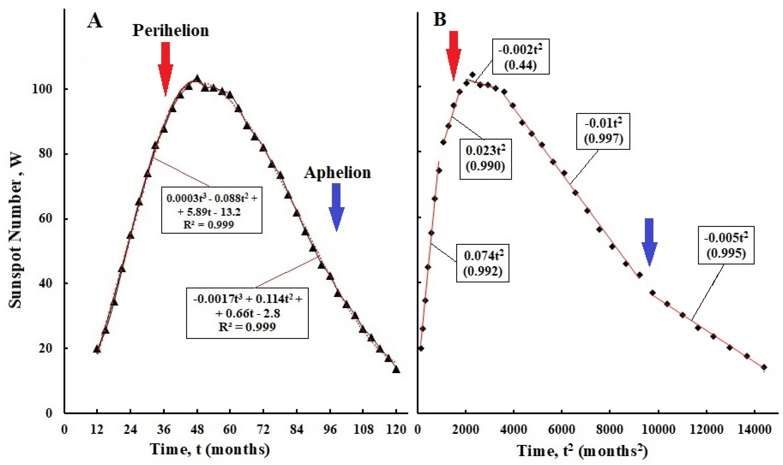
Figure 2.
A—Temporal variations: of the total magnetic moment of the Sun (μfull, μT/R3), SL9—fall of comet Shoemaker-Levy on Jupiter, blue and gray fields of rectangles—intervals of Jupiter’s motion above and below plane of solar equator (SE), respectively (upper panel); q—angle of solar dipole (μS) during polarity reversal in Hale cycle through quadrupoles (QS) at maxima of 21st and 22nd solar cycles (middle panel); W—number of sunspots in cycles 21, 22 and 23 (lower panel). B—strength of vertical solar magnetic field (Bd, upper panel); solar quadrupole (QS) in the 21st-24th solar cycles (middle panel); W—sunspot numbers in 21-24 SA cycles (lower panel), dates of Jupiter’s positions at perihelion and aphelion (vertical red and blue arrows), dates of Jupiter’s crossing of the SE plane (junction of the oblique red and blue arrows). A and B are adapted from [Livshits, 2006] and [Obridko, 2020], data on W and Jupiter from [Space Weather; Planets Jupiter].
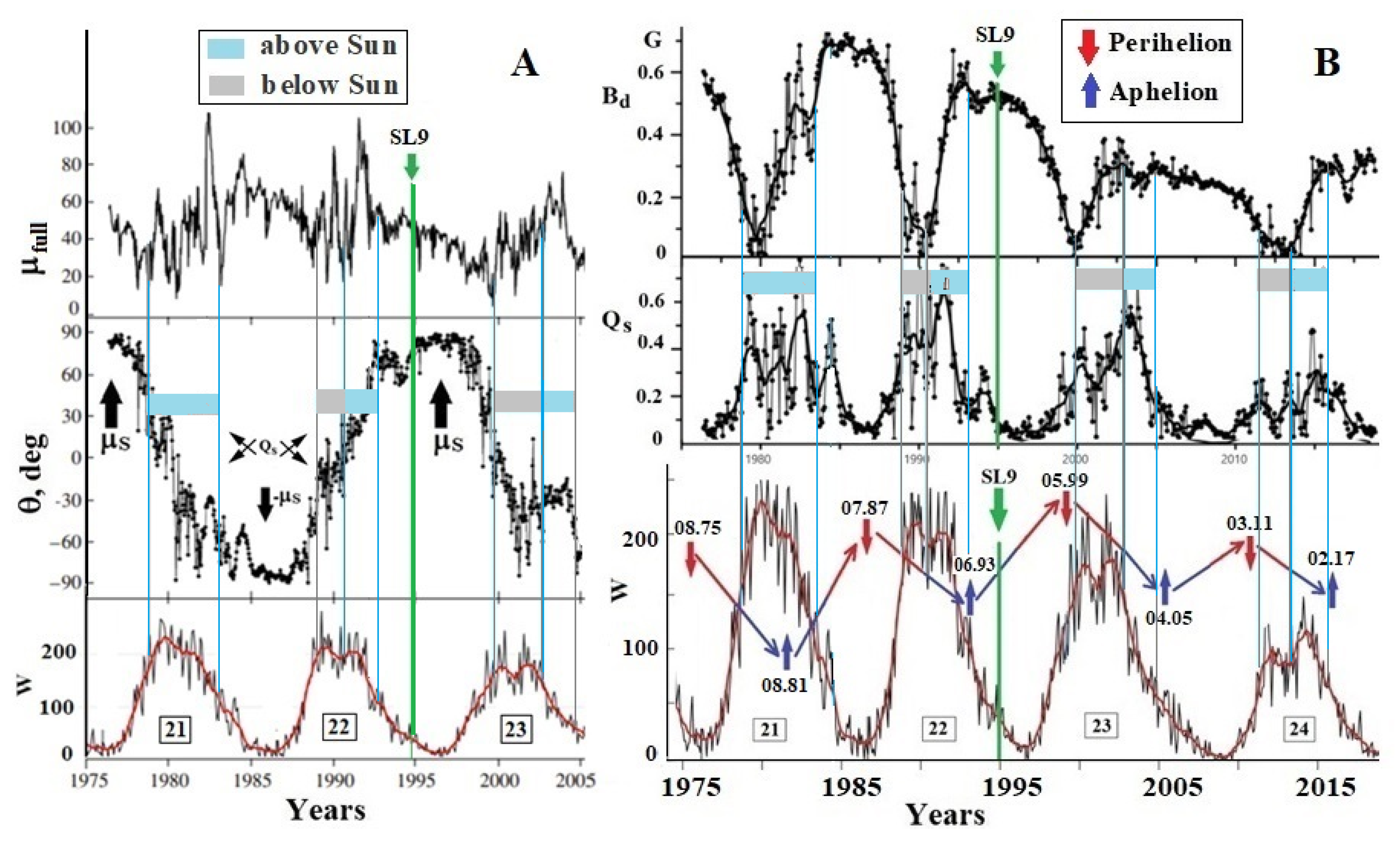
Figure 5.
Special points of Jupiter’s orbit in upper panel: perihelion and aphelion (red and blue arrows), intersection of orbit with SE plane (black arrow) from bottom-up (from gray field to blue one) and from top-down (from blue field to gray one); in middle panel: chronologies of variations in number of sunspots (W) and total magnetic fluxes (flux) in regular active regions (ARs) of northern and (N) and southern (S) hemispheres of Sun; in lower panel: chronologies of irregular ARs. The vertical red and blue lines in both panels mark positions of Jupiter’s perihelion and aphelion on W and flux chronologies in Schwabe cycles 23 and 24; double vertical multi-colored lines mark periods of Jupiter’s intersection with SE on cycles. The figure is adapted from [Zhukova, 2023].

Figure 6.
Annual global mean integrals of heat content anomaly estimates. A—upper ocean layer (0–700 m), intermediate layer (700–2000 m), deep and abyssal layer (z>2000 m). B—total heat entering the Earth system. 1 ZJ = 1021 J. A—adaptation of Figure 3.6 from [Johnson, 2023], B—of Figure 8 from [Schuckmann, 2023].
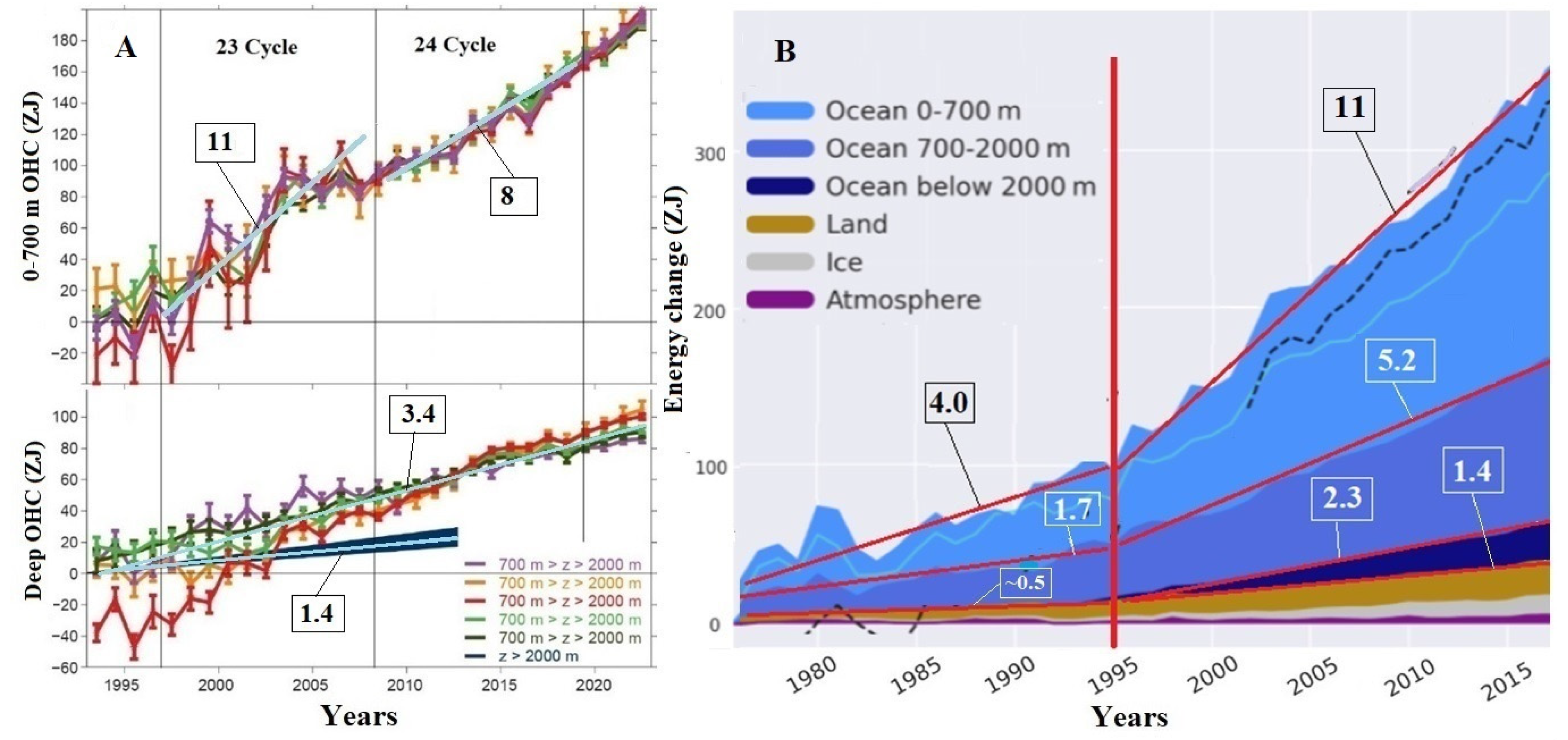
Figure 7.
A—Seasonal (3-month) thermal energy in upper 800 m of ocean compared to 1955–2006 average. B—Global annual mean anomalies in atmospheric heat content. The arrow marks the maximum of the El Niña event. C—Estimates of rate of total heat uptake by all ice sheets on Earth. 1 ZJ = 1021 J, k in frame (ZJ/yr). A—adapted from [Lindsey, 2023], B and C—adapted from Figure 4 and Figure 7 from [Schuckmann, 2023].
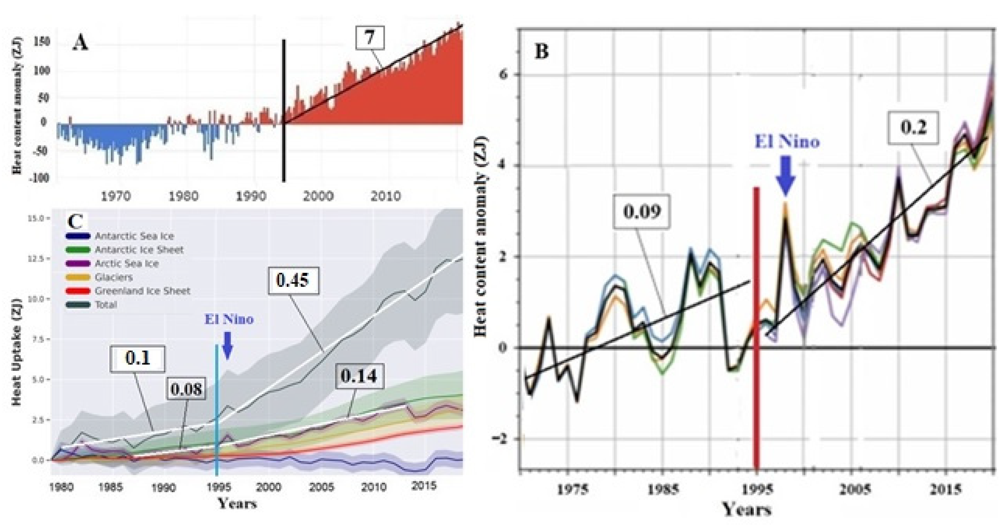
Figure 8.
A—satellite-based temperature of low atmosphere (Figure from [UAN]), the arrow marks maximum of El Niña phenomenon. B—Arctic sea ice minimum extents declined, satellite record, Adaptation of figure from [Blunden, 2020].
Figure 8.
A—satellite-based temperature of low atmosphere (Figure from [UAN]), the arrow marks maximum of El Niña phenomenon. B—Arctic sea ice minimum extents declined, satellite record, Adaptation of figure from [Blunden, 2020].
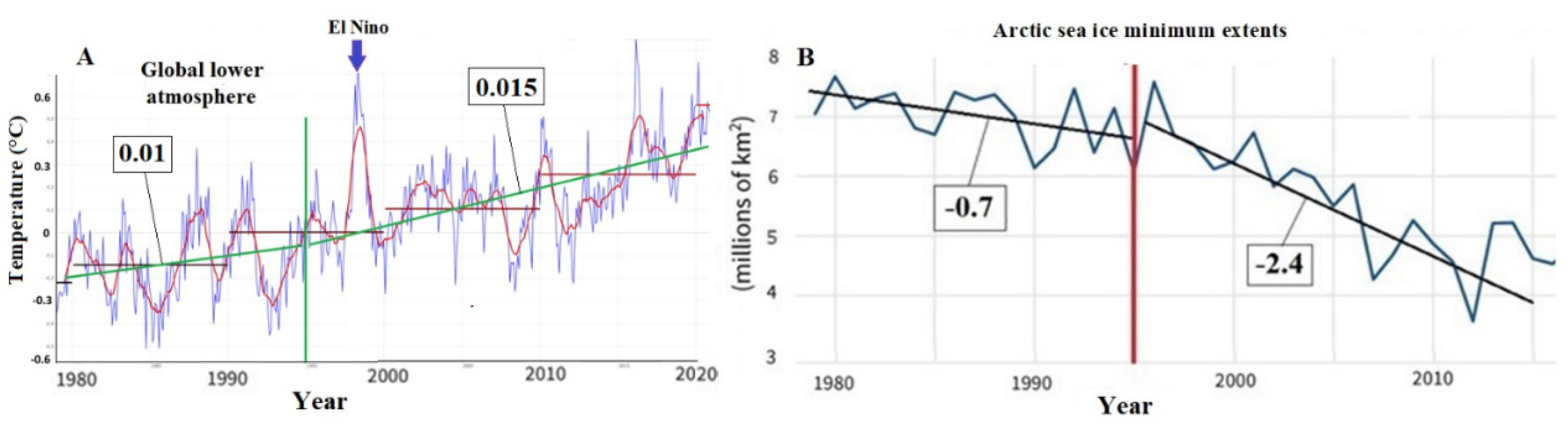
Figure 9.
A—Global mean surface air temperature anomalies (°C; base period 1991–2020) for (a) land only and (b) ocean only. B—Global mean annual total column water vapor anomalies. In k (kg m−2 yr−1) over ocean and land. The arrow marks the El Niña maximum. A and B adapted from Figure 2.1 and 2.25 from [Blunden, 2023].
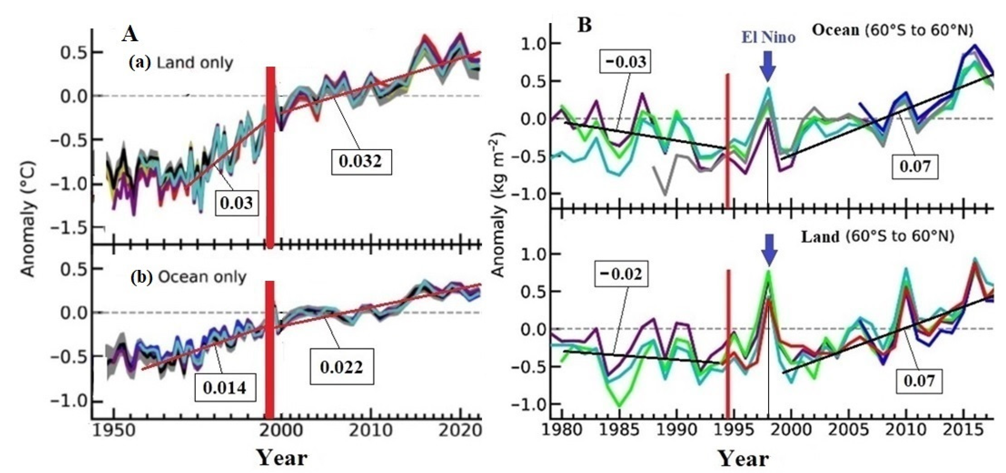
Figure 10.
A—Three-layer structure of Earth’s interior. In center is a solid iron core, around it is a liquid outer core with ring currents and convective electrochemical flows, above outer core is a mantle, which is penetrated by magnetic field lines of the ring currents. B—Diagram of geostrophic cylinders C(s) in the outer core, TC is a tangent cylinder. C—diagram of Earth’s structure. A and B—adaptation of Figure 1 and Figure 14 from [Landeau, 2022] and [Roberts, 2013].
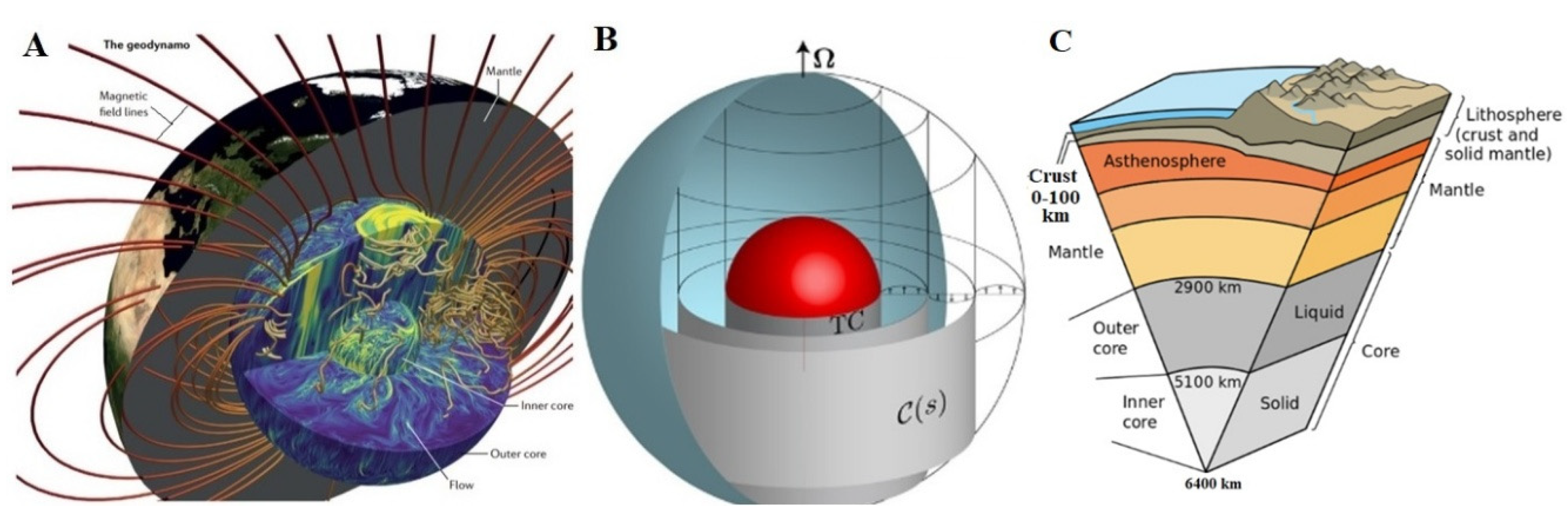
Figure 11.
South Atlantic Magnetic Anomaly. Points of impact of asteroid 65 Ma—1 (21°N, 89°W) and Tunguska meteorite in 1908—2 (60°N, 101°E).
Figure 11.
South Atlantic Magnetic Anomaly. Points of impact of asteroid 65 Ma—1 (21°N, 89°W) and Tunguska meteorite in 1908—2 (60°N, 101°E).
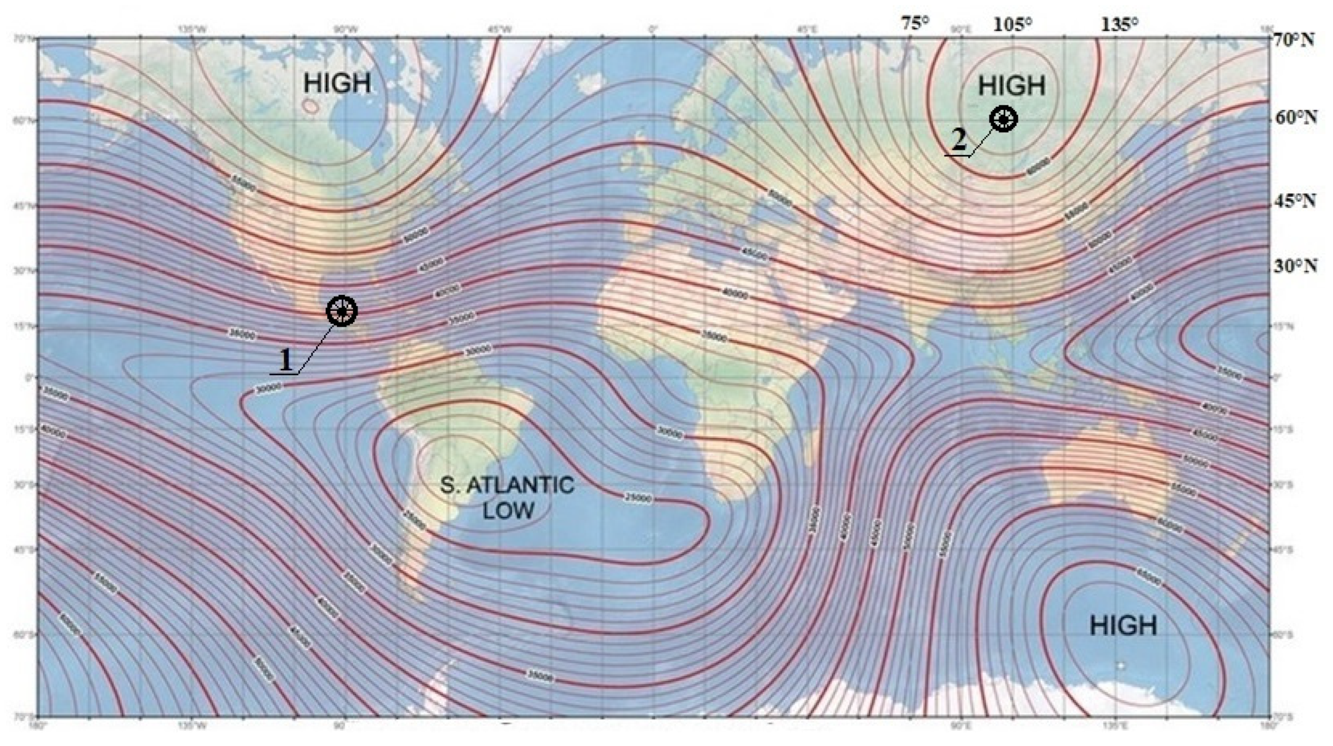
Figure 12.
A, B—Change in dipole moment of geomagnetic field. C—Average speed of the magnetic dipoles over each 5-year epoch, plotted at midpoint between epochs. A and C are adaptations of figures 5 and 4 from [Alken, 2021], B—data from World Data Center for Geomagnetism, Kyoto, http://wdc.kugi.kyoto-u.ac.jp/.
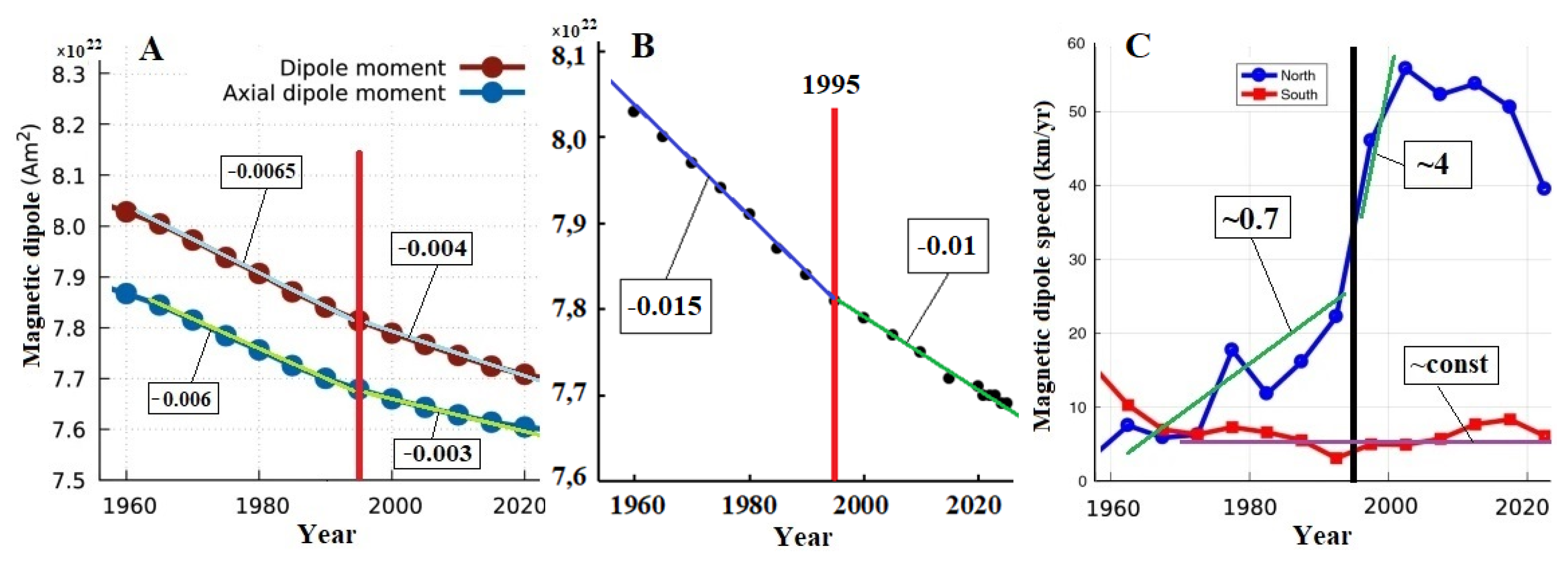
Figure 13.
A—Energy in terms of spatial power spectra of dipole field (left axis and blue dots) and non-dipole field (right axis and red dots) on Earth’s surface. B—Change in extent area of South Atlantic Magnetic Anomaly (SAA). C—Chronicles of radial components of the field, exiting from America and entering in Africa. Adaptation of Figures from [Pavón-Carrasco, 2016].
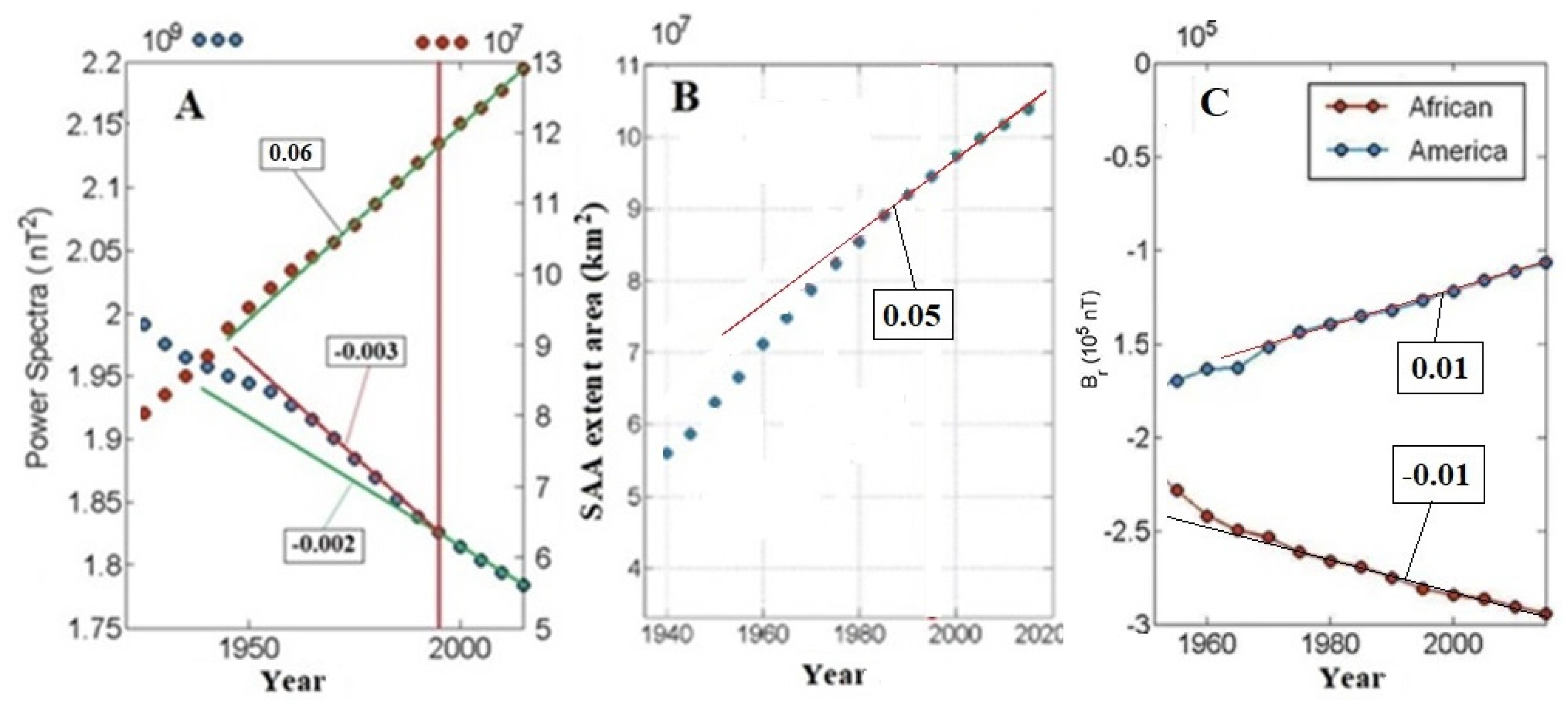
Figure 14.
A—Geochronology of virtual dipole moment. The red line is the mean values, gray field is scatter in different dimensions, their number is indicated by numbers. B—Blue and red arrows are global extinctions (GE), green arrow is Cambrian explosion of biodiversity (Cm). In the boxes are galactic years (GG), the purple lines are GG boundaries. C—Geochronology of Phanerozoic global temperature, the red line is envelope by mean values. Arrows are regular GE. Data for A are from [Biggin, 2009; Veselovskiy, 2024]; for B from [Biggin, 2003; Heunemann, 2013; Kulakov, 2019; Shcherbakova, 2021; Thallner, 2021], for C from [Kholmanskiy, 2024; Scotese, 2024].
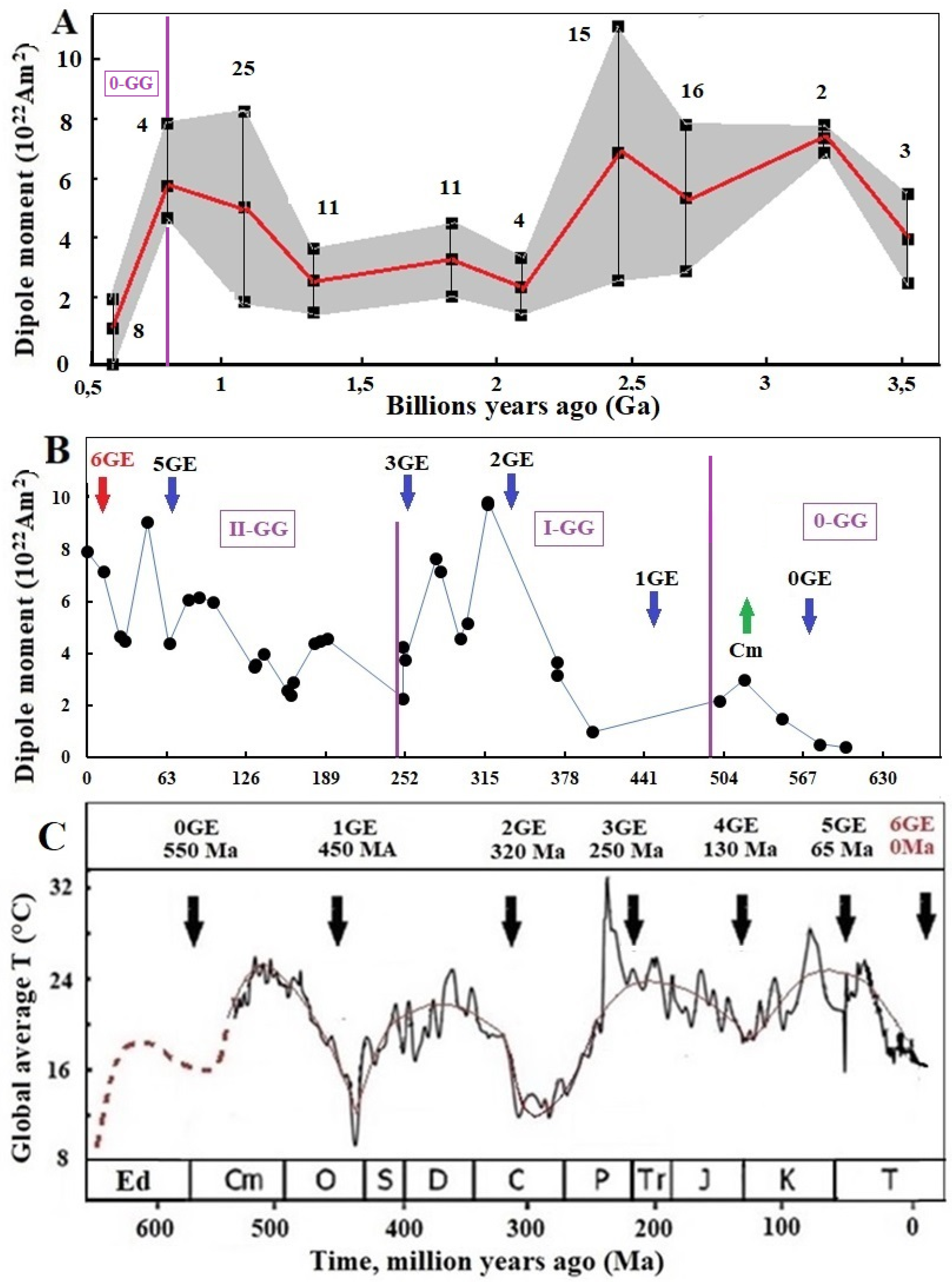
Figure 15.
Positions of continents within bulge (red line) during global extinction events (GE)—0 Ma (6GE), 65 Ma (5GE), 200 Ma (~4GE), 260 Ma (3GE), ~485 Ma (1GE) and ~550 Ma (0GE). Adaptation of figures 0–260 Ma from [Pétrélis, 2011], 485 Ma and 550 Ma from [Scotese, 2024; Paleozoic] and 635 Ma, 720 Ma from [Hoffman, 2017].
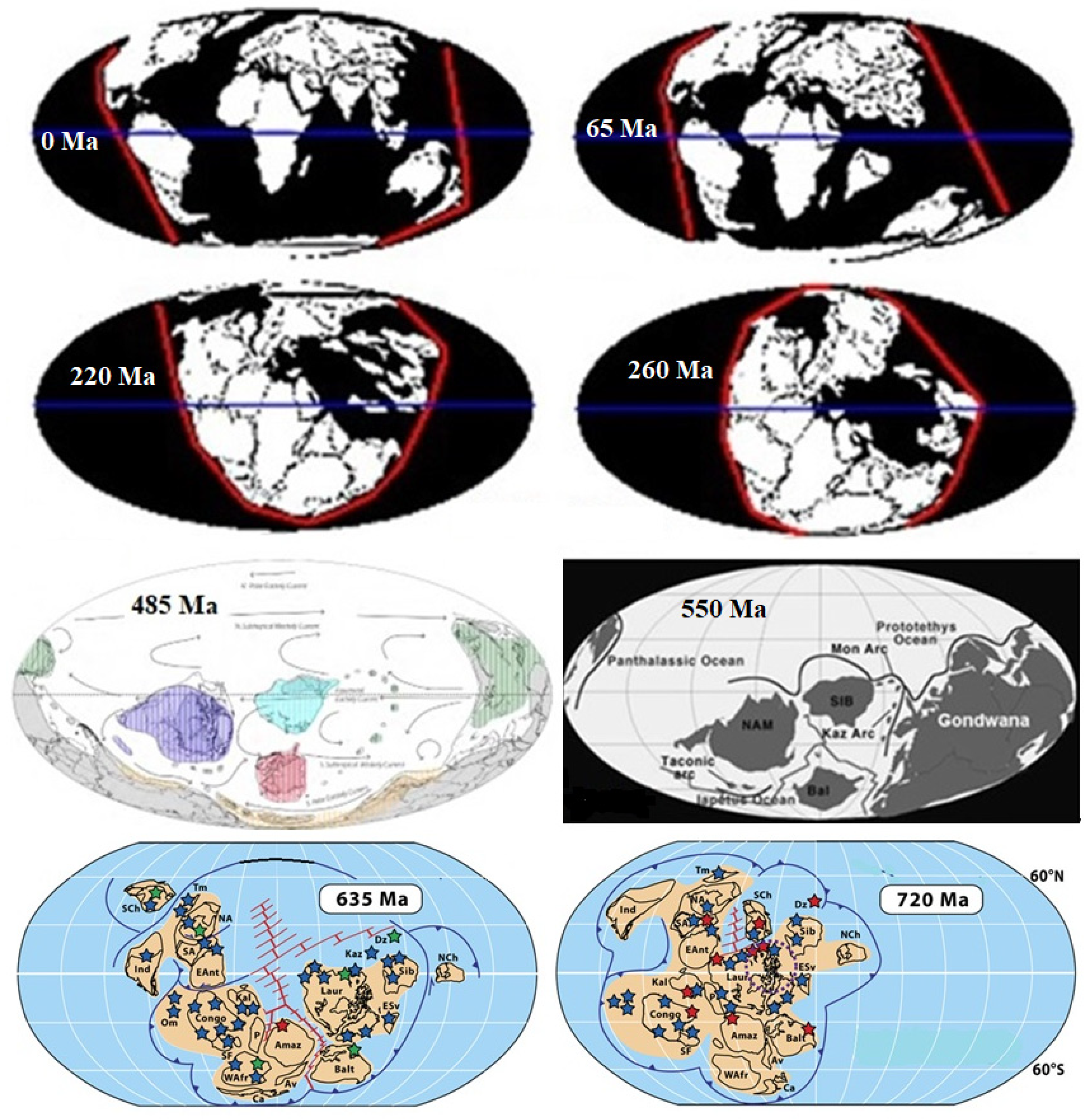
Figure 16.
Dependences of thermal conductivity coefficient (λ) of water (Аw) and quartz (Aq) on T and 1/Т (Bw, Bq). The arrow marks anomalous T for water (4°). The dotted lines in the figures are approximations by functions exp(EA/RT). The activation energies EA in kJ/mol are given in squares. The initial TDs λ for water are from [Thermalinfo] and quartz from [Nemilov, 2011].
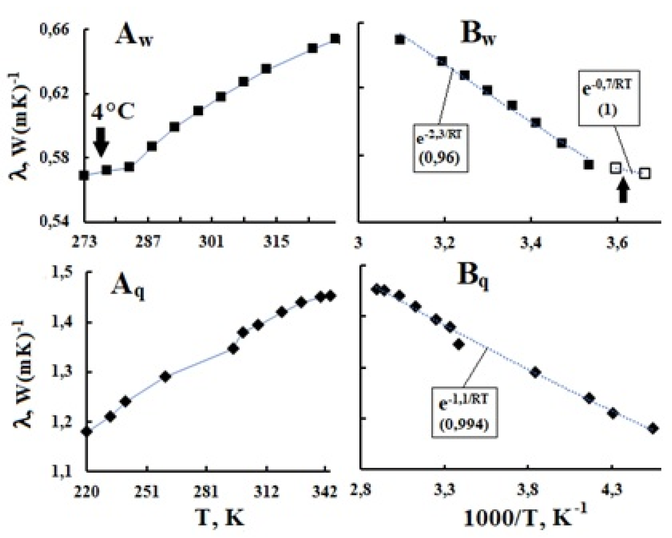
Figure 17.
A—Number of earthquakes with magnitude 6.0 and higher (1973-2011). B—Number of volcanic eruptions (1973-2011).
Figure 17.
A—Number of earthquakes with magnitude 6.0 and higher (1973-2011). B—Number of volcanic eruptions (1973-2011).
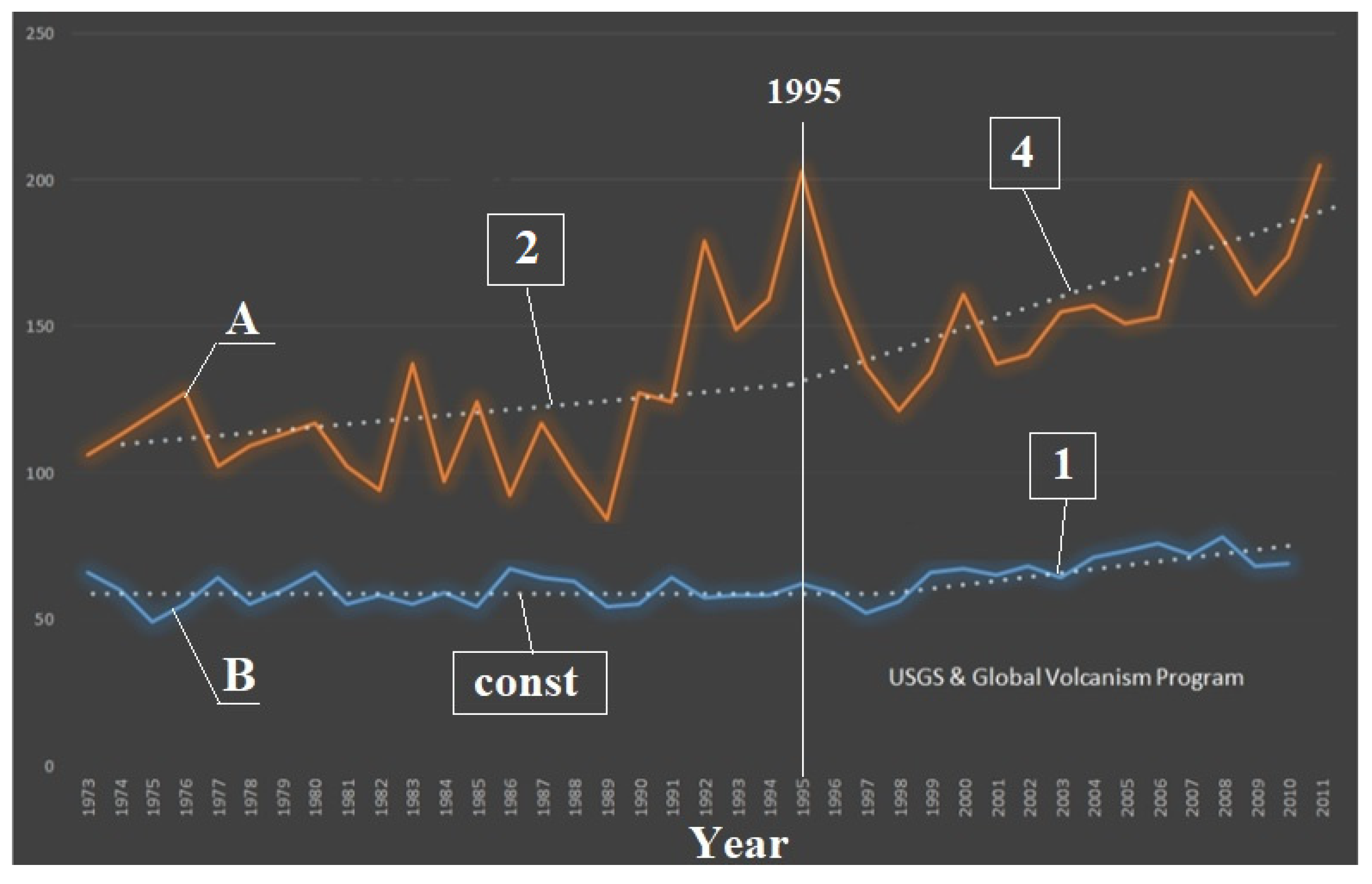
Figure 18.
Global Living Planet Index (LPI) by ecosystem type from 1970 to 2020. Adapted Figure 1.4 from [WWF, 2024].
Figure 18.
Global Living Planet Index (LPI) by ecosystem type from 1970 to 2020. Adapted Figure 1.4 from [WWF, 2024].
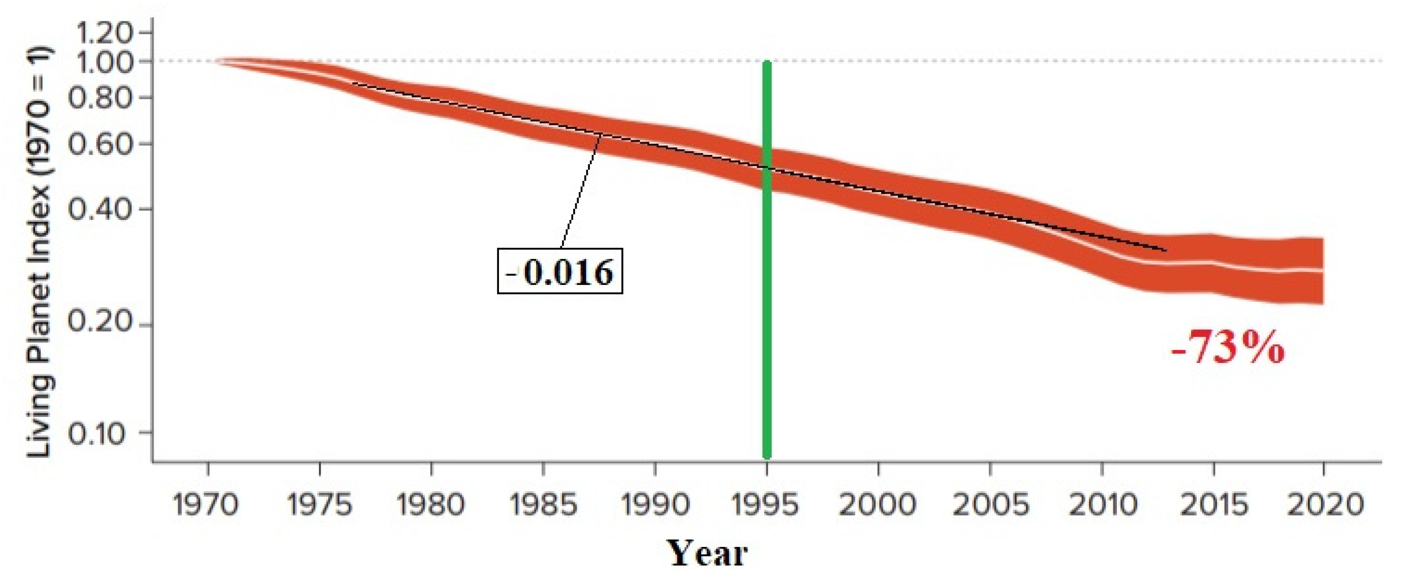
Figure 19.
A—Annual number of recorded weather-related natural disasters occurring in SA cycles 21–24. B—Histogram of peer-reviewed papers on cryogenic glaciation by discipline. A and B are adapted from [Global reported] and [Hoffman, 2017], respectively.
Figure 19.
A—Annual number of recorded weather-related natural disasters occurring in SA cycles 21–24. B—Histogram of peer-reviewed papers on cryogenic glaciation by discipline. A and B are adapted from [Global reported] and [Hoffman, 2017], respectively.
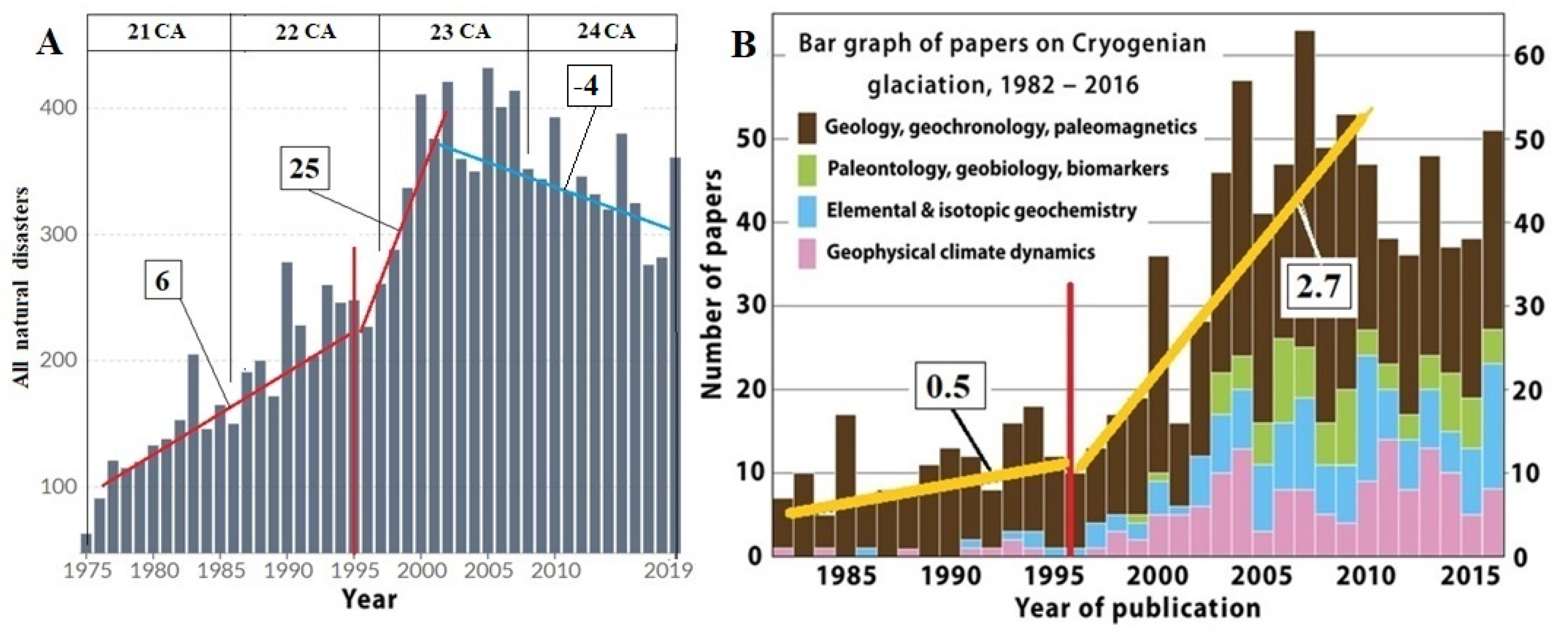
Figure 20.
A—graphs of growth of Earth’s population (1) and changes in human creative activity, summing up useful ideas, discoveries and inventions at each point in time; the arrow Ω marks the beginning of human combustion of coal, oil and gas [Kholmansky, 2019a]. B—Idea Flow Index for all sciences and all regions [Cauwels, 2020] and the location of the 18th, 19th and 20th SA cycles [Dodson, 1974]. C—exponential growth in the number of Internet sites on World Wide Web after 1995 (Internet Live Stats).
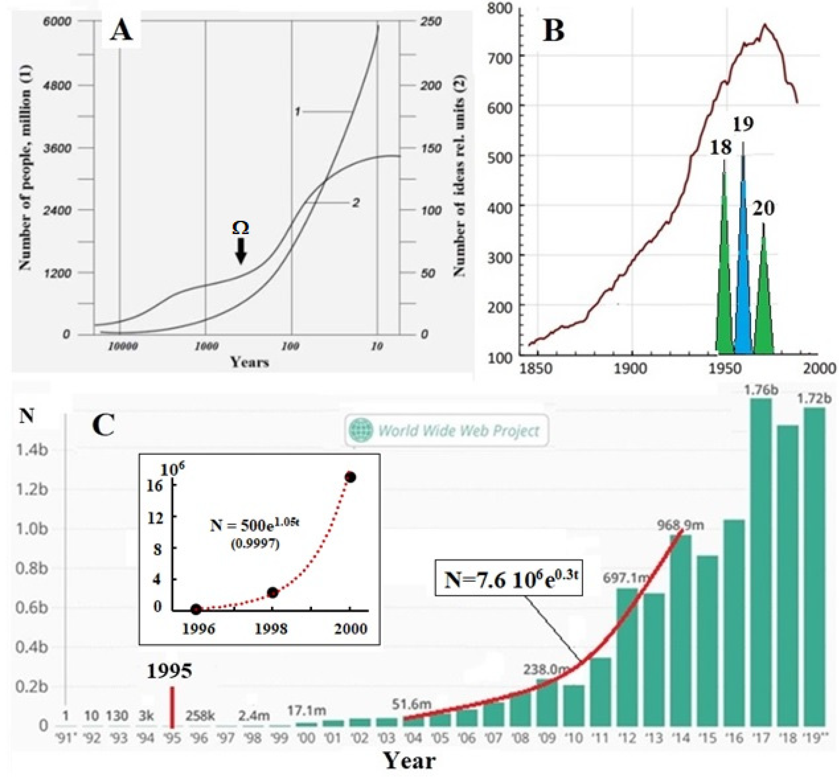
Figure 21.
Alzheimer’s disease mortality rates per 100,000 population. A—in Michigan. Data from [https://www.mdch.state.mi.us/osr/deaths/AlzheimersCrudeRatesTrends.asp]. B—for Italy as a whole for men and women, broken down by age group. Figure adapted from [Bezzini, 2024].
Figure 21.
Alzheimer’s disease mortality rates per 100,000 population. A—in Michigan. Data from [https://www.mdch.state.mi.us/osr/deaths/AlzheimersCrudeRatesTrends.asp]. B—for Italy as a whole for men and women, broken down by age group. Figure adapted from [Bezzini, 2024].
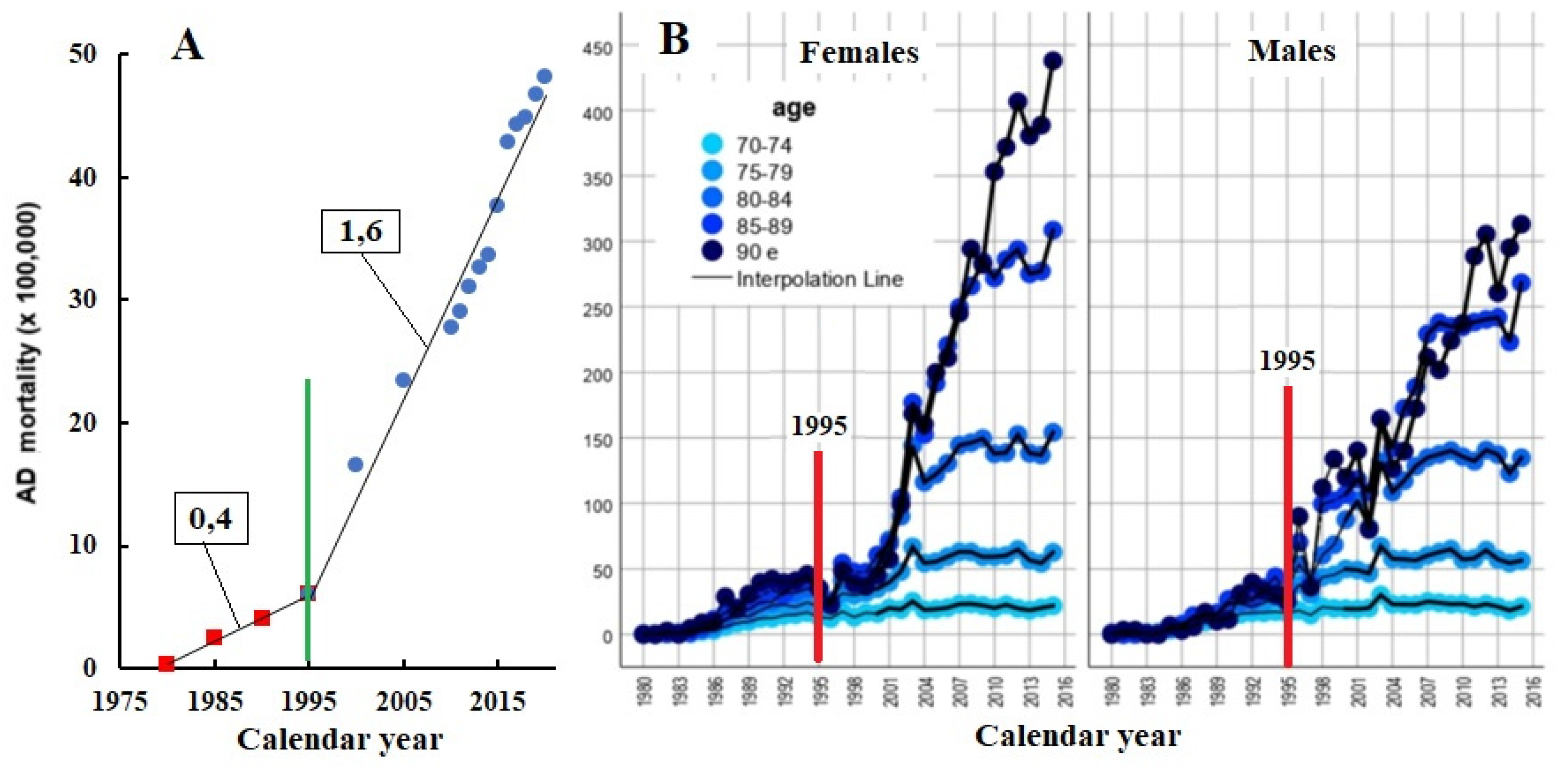

Table 1.
Orbital radii (RP), periods (Y), masses (Mass), dipole moments (μ) of the Sun and planets. Ratios of tidal (Pт) and magnetic (Pμ) effects of the planets (Pμ/Pt). Parameters for Earth are 1.
Table 1.
Orbital radii (RP), periods (Y), masses (Mass), dipole moments (μ) of the Sun and planets. Ratios of tidal (Pт) and magnetic (Pμ) effects of the planets (Pμ/Pt). Parameters for Earth are 1.
| Sun, Planet | Y (year) (yer) | Mass | m*) | RP (AU) | Tides | Magnetic | Pm/Pt |
| Sun | - | 3.3 105 | 4.4 106 | 0 | - | - | - |
| Mercury | 0.24 | 0.06 | 4.7 10-4 | 0.31-0.47 | 0.55-1.85 | 7 10-3 | 10-3 |
| Venus (V) | 0.62 | 0.82 | 1.0 10-5 | 0.72 | 2.2 | 2.7 10-5 | 10-5 |
| Earth (E) | 1 | 1 | 1 | 1 | 1 | 1 | 1 |
| Mars | 1.88 | 0.11 | 2.6 10-5 | 1.52 | 0.03 | 7 10-6 | 10-4 |
| Jupiter (J) | 11.86 | 318 | 1.9 104 | 4.95-5.46 | 2.0-2.7 | 140 | 70 |
| Saturn | 164.8 | 95 | 576 | 9.54 | 0.11 | 0.66 | 6 |
| Uran | 84 | 14.5 | 50 | 19 | 2 10-3 | 7 10-3 | 3 |
| Neptun | 164 | 17,1 | 30 | 30 | 0.5 10-3 | ~1 10-3 | 2 |
*)—значения m из [Magnetic dipoles; Ness, 1986].
Disclaimer/Publisher’s Note: The statements, opinions and data contained in all publications are solely those of the individual author(s) and contributor(s) and not of MDPI and/or the editor(s). MDPI and/or the editor(s) disclaim responsibility for any injury to people or property resulting from any ideas, methods, instructions or products referred to in the content. |
© 2025 by the authors. Licensee MDPI, Basel, Switzerland. This article is an open access article distributed under the terms and conditions of the Creative Commons Attribution (CC BY) license (http://creativecommons.org/licenses/by/4.0/).
Copyright: This open access article is published under a Creative Commons CC BY 4.0 license, which permit the free download, distribution, and reuse, provided that the author and preprint are cited in any reuse.


