
Submitted:
22 April 2025
Posted:
22 April 2025
You are already at the latest version
Abstract
In recent years, rapid progress in autonomous driving has been achieved through advances in sensing, control, and learning. However, as the complexity of traffic scenarios increases, ensuring safe interaction among vehicles remains a formidable challenge. Recent works combining artificial potential fields (APF) with game-theoretic methods have shown promise in modeling vehicle interactions and avoiding collisions. Yet, these approaches often suffer from overly conservative decisions or fail to capture the nonlinear dynamics of real-world driving. To address these limitations, we propose a novel framework that integrates mean field game (MFG) theory with model predictive control (MPC) and quadratic programming (QP). Our approach leverages the aggregate behavior of surrounding vehicles to predict interactive effects and embeds these predictions into an MPC-QP scheme for real-time control. Simulation results in complex driving scenarios demonstrate that our method achieves multiple autonomous driving tasks while ensuring collision-free operation. Furthermore, the proposed framework outperforms popular game-based benchmarks in terms of achieving driving tasks and producing fewer collisions.
Keywords:
Autonomous vehicle
; interactive driving
; risk potential field
; model predictive control
1. Introduction
In recent years, human-robot interactions (HRI) has raised high attention from public [1,2]. Among the HRIs, the field of autonomous driving has witnessed remarkable progress driven by advancements in sensing technologies [3,4,5,6], planning [7,8,9] and control systems [10,11], and machine learning techniques [12,13,14]. Despite these breakthroughs, ensuring safe and efficient interactions among vehicles in complex traffic scenarios remains a formidable challenge. As autonomous vehicles (AVs) are increasingly deployed in mixed traffic environments alongside human-driven vehicles (HDVs) [15], the ability to predict and respond to the actions of surrounding agents becomes crucial for collision avoidance and smooth operation.
Traditional methods that combine artificial potential fields (APF) with game-theoretic models have demonstrated promise in modeling vehicle interactions and preventing collisions [16,17,18]. However, these approaches often result in overly conservative control decisions or fail to accurately capture the nonlinear dynamics inherent in real-world driving. For instance, such methods may lead to unnecessarily cautious maneuvers that compromise traffic efficiency or may not adapt adequately to rapidly changing traffic conditions.
Learning-based methods have gained considerable attention [19,20,21,22,23,24,25] due to their ability to capture complex vehicle behaviors. However, these techniques typically require vast amounts of training data, which demands significant computational resources. Furthermore, since they often have an unseen decision-making process [26], thus their decision-makings lack transparency and interpretability. Recently, large language models (LLMs) also becomes an attracting field, which enables agent to recognize the textual information [27,28]. However, LLMs sometimes are without precision in low-level decision-making, even they can reasonably give a proper high-level commands.
To address these challenges, we propose a novel framework that integrates mean field game (MFG) theory [29] with model predictive control (MPC) integrated with quadratic programming (QP) [30]. In our approach, MFG theory is used to capture the aggregate behavior of surrounding vehicles. Instead of modeling each vehicle individually, MFG approximates the interactions of a large population of agents by a mean field term, which represents the average influence of all vehicles. This not only reduces the complexity of the multi-agent system but also preserves essential interactive dynamics, which are critical for safety in dense traffic environments. On the other hand, MPC provides a receding-horizon framework that continuously updates the control inputs based on real-time state measurements and predicted future behavior. By linearizing the vehicle dynamics around a nominal trajectory and formulating the control problem as a QP, we can efficiently solve the resulting optimization problem even in the presence of constraints and nonlinearities. By doing so, the framework dynamically adjusts the AV’s control inputs in real time, thereby balancing safety and efficiency across various driving tasks. Our approach offers several significant contributions:
- The proposed framework utilizes mean field approximations to capture the aggregate behavior of surrounding vehicles, providing a more accurate and computationally efficient representation of interactive driving scenarios.
- By integrating these mean field predictions into a receding-horizon MPC-QP framework, our framework effectively handles the nonlinear dynamics of vehicles while ensuring real-time computation of optimal control actions.
- Extensive simulation results demonstrate that our framework not only guarantees collision-free operation but also produces smoother trajectories and enhanced overall traffic performance compared to existing game-based approaches.
The remainder of this paper is organized as follows. Section 2 reviews related works and their limitations. Section 3 describes the system model and presents our vehicle dynamics. Section 4 details the proposed MFG integrated MPC-QP framework, including the formulation of the optimization problem and the solution approach. Finally, Section 5 presents simulation results demonstrating the efficacy of the proposed method, and Section 6 concludes the paper.
2. Related Works
2.1. Challenges in Interactive Decision-Making
Interactive decision-making in autonomous driving is particularly challenging due to the highly dynamic and uncertain nature of traffic environments [31,32,33]. Vehicles must continually predict and respond to the behavior of surrounding agents while dealing with nonlinear vehicle dynamics and measurement uncertainties [34,35,36,37]. As the number of interacting vehicles increases, the computational burden associated with modeling each individual interaction becomes prohibitive. Consequently, ensuring safe, efficient, and smooth vehicle maneuvers in dense traffic remains a formidable problem.
2.2. Shortcomings of Current Game-Based Approaches
Game-based approaches have been widely employed to model the strategic interactions among vehicles, providing a structured framework to predict the actions of other drivers. In the case of Stackelberg games [38,39], the AV is modeled as the leader that anticipates the optimal responses of the followers. However, this formulation typically relies on the assumption of perfect rationality, which is not always valid in real-world scenarios, and tends to yield overly conservative decisions that sacrifice traffic efficiency. Consequently, Stackelberg games heavily depend on accurate predictions of other participants’ decisions. Moreover, the hierarchical structure of Stackelberg models may not scale well when multiple vehicles are involved; for instance, an additional game-ordering mechanism is required when using Stackelberg games for multi-vehicle interactions [40].
On the other hand, Nash game formulations treat all vehicles symmetrically by seeking a simultaneous equilibrium [41]. Although Nash approaches capture the mutual influence among agents, they often suffer from the existence of multiple equilibria, complicating the selection of a unique solution in real time. For example, Nash approaches are typically applied only to maintain a game process for a single focused vehicle in a two-vehicle game [42,43], which neglects broader game-based interactions with other vehicles. In addition, the computational complexity associated with solving for a Nash equilibrium in high-dimensional and nonlinear settings can be significant. These limitations in both Stackelberg and Nash formulations have motivated our focus on developing more scalable game-based approaches that offer an interpretable framework for interactive decision-making despite their shortcomings.
MFG theory provides a promising alternative by approximating the aggregate behavior of a large population of vehicles through a mean field term. This approach alleviates the need to model each interaction individually and addresses the scalability issue inherent in traditional game formulations. However, previous works on MFG integrated with autonomous driving fail to conduct simulations among multiple driving scenarios, compare with other game-based approaches, and connect with the control optimization problems [29,44]. By integrating MFG with MPC-QP, our framework effectively captures the collective dynamics of surrounding vehicles while leveraging a receding-horizon optimization scheme that handles nonlinear vehicle dynamics in real time [45,46,47]. This integration not only mitigates the overly conservative nature of Stackelberg games and the computational complexity of Nash games, but also yields a more flexible and robust solution for interactive driving.
3. System Overview
Framework Description:
Figure 1 provides a schematic illustration of our overall approach. In the left-hand portion, the multi-vehicle scenario is shown, where an AV navigates within a bounded environment alongside several surrounding vehicles (SVs). Potential collision zones are highlighted by overlapping or convergent trajectories. Moving to the central portion, our MFG module is depicted. In this module, the states of all vehicles (except the one being controlled) are aggregated to compute a mean field correction term, . This correction approximates the collective influence of the SVs, and it is dynamically adjusted based on environmental constraints and historical proximity data, enabling the correction to evolve over time and accurately reflect real-time interactions among vehicles. In the right-hand portion, these MFG predictions are integrated into a MPC formulation, which is solved via QP. The MPC-QP optimization minimizes a cost function—expressed in compact matrix form—that accounts for trajectory tracking, control effort, and safety constraints such as collision and boundary penalties, all subject to the vehicle’s dynamic model. The resulting control commands ensure that the AV can safely and efficiently navigate through complex, multi-participant traffic scenarios.
4. Methodology
We consider a multi-vehicle system composed of one AV and HDVs operating in a bounded environment , for example, a rectangular area with boundaries at , , , and . The environment constraints are integrated into our control design to ensure that vehicles remain within safe operational limits.
For each vehicle i, the state is defined as
and the control input is
The dynamics follow the bicycle model:
The joint state vector for all vehicles is
4.1. Interactive Prediction via MFG
To capture vehicle interactions, the instantaneous cost for vehicle i is defined as
where and are positive-definite matrices. In addition, to capture the influence of surrounding vehicles and potential collision risks, we define an interaction cost
and a collision penalty term
where is a smooth penalty function. Thus, the total cost over the horizon T is
To reduce the complexity of modeling individual pairwise interactions in multi-participant scenarios, our framework employs MFG theory. In our implementation, each vehicle contributes to a density field over the road surface. The contribution of vehicle i is modeled as a Gaussian function:
where is the intensity and , denote the spatial spreads. The overall density field is computed as
The MFG module computes an aggregate correction term by applying a mean field operator:
which is then used to update the reference state:
This process enables the controller to dynamically adjust for interactive effects based on both the real-time density field and environmental constraints.
Figure 2 illustrates our multi-vehicle simulation results at four distinct key times. Each row of subplots corresponds to one of these times, capturing significant moments in the simulation, such as early maneuvers or congested intervals. In every row, the left subplot depicts the traffic scene, where each vehicle is rendered as a colored polygon, sized and oriented according to its real-world dimensions and heading. These polygons highlight potential collision zones by overlapping or converging.
Moving to the right, the next three columns show the mean field game (MFG) density fields at the current time and two future offsets (for example, and ). These density fields are visualized using a color map, with warmer regions indicating higher vehicle density and cooler regions indicating lower density. By comparing rows and columns, one can observe how congested regions emerge, shift, or dissipate based on each vehicle’s movement and interaction.
The integration of these density fields with the traffic scenes underscores how our MFG module predicts and tracks the evolving distribution of vehicles in real time. The AV leverages these density predictions within our MPC-QP control framework, thereby adapting its trajectory and control actions to avoid high-density or high-risk areas. This dynamic approach ensures that the AV can safely and efficiently navigate through complex, multi-participant driving environments.
4.2. MPC-QP Formulation with Environmental and Safety Constraints
The MPC problem for each vehicle is formulated as
subject to the nonlinear dynamics (3) and the environmental constraint
Additionally, vehicle dynamic constraints such as acceleration and steering limits are enforced.
To solve (13) efficiently, we linearize the dynamics about a nominal trajectory
:
with
The QP is then formulated as
where the decision variable is
The Hessian matrix is defined as
where is the terminal cost weight. The gradient vector is
Each term in (18) reflects the propagation of control variations through the linearized dynamics, while (19) captures the deviation from the desired trajectory.
The optimal control correction is computed as
and the final control input is updated via
Our integrated framework combines the MFG prediction, MPC-QP optimization, and safety and environmental constraints into a unified control process. In every receding-horizon cycle, the following steps are executed:
|
Algorithm 1: Extended MFG Integrated MPC-QP Algorithm with Environmental and Safety Constraints
|
|
Figure 3.
Flowchart of the integrated MFG-MPC-QP framework for two scenarios: lane change and intersection negotiation.
Figure 3.
Flowchart of the integrated MFG-MPC-QP framework for two scenarios: lane change and intersection negotiation.
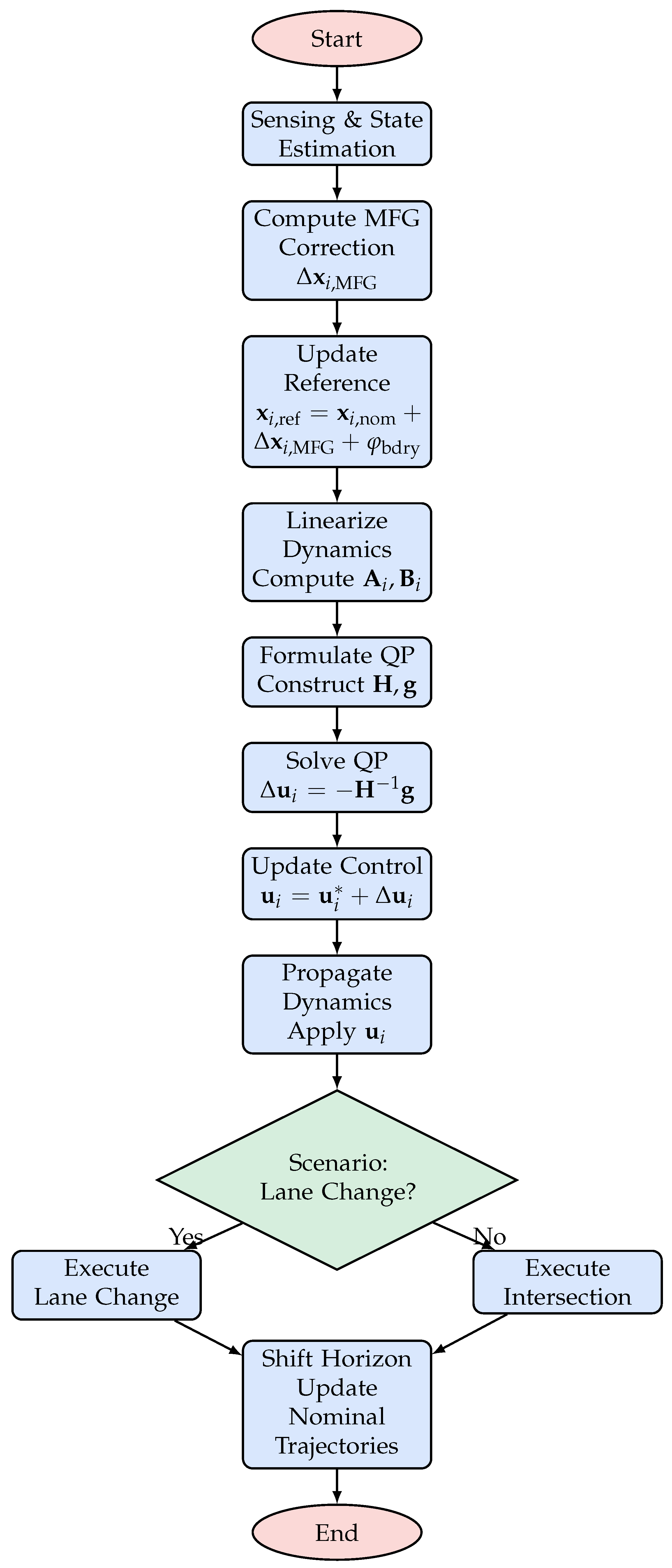
Algorithm Explanation: At each time step, every vehicle first computes a mean field correction that aggregates the influence of all other vehicles. This term, along with a boundary penalty enforcing environmental constraints, updates the reference state. The vehicle dynamics are then linearized about a nominal trajectory to obtain the Jacobian matrices and . Using these matrices, the QP problem is constructed via the Hessian and gradient , which encapsulate both tracking and control effort costs. The QP is solved to yield an optimal control correction , and the final control input is updated. This process is executed in a receding-horizon fashion to continuously adapt to real-time interactions and ensure safety, including collision avoidance via the penalty .
The following flowchart summarizes our approach for two typical scenarios: lane change and intersection negotiation. The flowchart is drawn using TikZ with SCI-inspired colors.The flowchart (Figure ) illustrates the major steps of our integrated framework.
- Start: This is the initialization step where the system loads all sensor data, initial vehicle states, and environmental parameters. The controller is set up to begin the receding-horizon control loop.
- Sensing & State Estimation: In this step, all vehicles (both the AV and HDVs) gather sensor data (e.g., from LiDAR, cameras, radar) to estimate their current states (position, velocity, heading). Accurate state estimation is critical for reliable prediction and control.
- Compute MFG Correction: The MFG module processes the states of all vehicles (except the one under consideration) to compute an aggregate correction term, . This term approximates the collective influence of surrounding vehicles, reducing the complexity of pairwise interaction modeling. It is then used to update the nominal reference state, so that the adjusted reference becomesthereby ensuring that the control policy dynamically incorporates real-time interactive effects.
- Update Reference: The nominal reference state is updated by incorporating the MFG correction along with a boundary penalty that accounts for the proximity to the environment boundaries. This yields the new reference state:
- Linearize Dynamics: The vehicle’s nonlinear dynamics (given by the bicycle model) are linearized around the nominal trajectory . The Jacobian matrices and capture the sensitivity of the state with respect to state and control inputs, respectively.
- Formulate QP Matrices: Using the linearized model, the Hessian matrix and gradient vector for the QP are constructed. Specifically, is computed by accumulating the termsand the gradient is given bywhere is the terminal cost weight matrix. These matrices encapsulate the tracking errors, control efforts, and indirectly include collision penalties from .
-
Solve QP: The quadratic programming problem is solved to obtain the optimal control correction:This step yields the necessary adjustment to the nominal control inputs to reduce the overall cost.
-
Update Control: The control input is updated by adding the correction term to the nominal control:This new control command is what is applied to the vehicle.
- Propagate Dynamics: The updated control inputs are applied to the nonlinear dynamics model to propagate the vehicle states forward. Additionally, environmental constraints are enforced to ensure that all vehicle states remain within the designated region .
- Scenario Decision: A decision node determines the driving scenario (e.g., lane change or intersection negotiation) based on the current state and predicted vehicle interactions. This decision may trigger additional scenario-specific maneuvers.
- Execute Maneuver: Depending on the scenario decision, the system executes the corresponding maneuver—either a lane change or an intersection negotiation—adjusting the control inputs as necessary.
- Shift Horizon: After control actions are applied and states are updated, the prediction horizon is shifted forward. The nominal trajectories are updated, and the process repeats in a receding-horizon fashion.
- End: The control loop terminates when the driving task is complete or when the specified time horizon is reached.
5. Experimental Evaluation
The simulations were conducted to evaluate the safety, stability, and efficiency of the proposed method. They were executed on a computer running Ubuntu 18.04.6 LTS, equipped with a 12th-generation, 16-thread Intel® Core™ i5-12600KF CPU, an NVIDIA GeForce RTX 3070Ti GPU, and 16 GB of RAM. All simulation results were generated using MATLAB R2024b.
To verify the effectiveness of our proposed MFG-based MPC-QP, we designed four distinct simulation scenarios that reflect typical interactive driving involving both HDVs and AVs. In the first scenario, the AV initiates interactive driving with surrounding HDVs in an irregular environment. In the second scenario, the AV navigates a two-lane highway while two surrounding AVs are positioned around the host AV; here, the AV must perform a lane change while maintaining a safe distance from the surrounding AVs. In the third scenario, the number of surrounding AVs is increased to three, with all other conditions remaining the same as in the second scenario. In the fourth scenario, the AV is required to reach a target point across an intersection while the surrounding HDVs follow fixed routes. To underscore the superior performance of the proposed method, we compared it against other popular benchmark algorithms in the last three scenarios.
5.1. Verification for Scenario 1
In this first scenario, Figure 4 illustrates our first test scenario in a top-down view. The environment is bounded by fences in the upper and lower sections, with decorative trees placed near each corner. In the lower-left portion, the AV is shown traveling from left to right, indicated by the dashed road boundary. Several HDVs appear at different positions and orientations: one moves vertically down near the upper-left fence, another navigates horizontally from the right fence toward the center, and an additional HDV heads northward near the middle of the scene. This setup emphasizes potential crossing paths and showcases how the AV and HDVs share the same road space while maneuvering around obstacles and boundaries.
Figure 5(a) displays the position of each vehicle at discrete time steps, plotting their x-y coordinates and linking them to reveal their paths over time. Vehicles moving primarily in the vertical direction appear as nearly straight vertical lines, whereas those traveling horizontally show up as elongated horizontal tracks. The intersection of these paths highlights potential conflict points, yet collision avoidance ensures no overlapping positions occur at the same time.
Figure 5(b) shows the corresponding density field at several key instants. The color scale transitions from yellow/white to red . Each vehicle contributes a Gaussian-like distribution to the field, which is then summed and normalized. Over the progression of time frames, one can observe how the distribution evolves, reflecting changes in vehicle positions and velocities. This time-evolving density field supports collision-free navigation by allowing the decision-making module to anticipate and react to congested zones before they become hazardous.
Figure 6 presents the evolution of two key indicators over a six-second window: the average speed of all vehicles and the cumulative collision count. The horizontal axis (T) indicates the discrete time steps in seconds. As the simulation progresses, each second’s average speed is computed by taking the mean of the current speeds across all vehicles. Meanwhile, the collision count is accumulated whenever two vehicles come within a specified safety distance. This plot demonstrates the system can maintain stable average speeds while keeping the collision count at zero. A gradual decrease or fluctuation in speed may occur as vehicles maneuver to avoid potential conflicts, underscoring the trade-off between efficiency and safety.
Figure 7 shows a two-lane road scene with dotted lane markers. The host AV is positioned in the lower lane, while another AV and an additional vehicle occupy the upper lane. The gray rectangle represents the drivable region, and each lane is bounded by dashed lines. The host vehicle’s objective is to switch from its current lane to the target lane, coordinating with the other vehicles to avoid collisions or abrupt maneuvers. By adjusting speed and lateral motion, the host vehicle ensures that its lane change occurs safely, even in the presence of adjacent vehicles in the upper lane. This setup underscores how lane-changing decisions must account for the trajectories of surrounding vehicles, balancing efficiency and collision avoidance in real time.
Figure 8 shows the x-y trajectories of three autonomous vehicles (each color-coded: blue, green, and red) under three different approaches. In the left panel, our method produces smooth and collision-free paths without any abrupt or backward motion. Each vehicle converges toward its desired lane or target position in a balanced way, demonstrating how the MFG correction effectively captures multi-vehicle interactions, and the MPC framework ensures efficient, real-time trajectory adjustments. By contrast, the center panel APF+Stackelberg and right panel APF+Nash reveal that both methods sometimes force a vehicle to move backward to avoid collisions, which can be a poor choice in real traffic. In the Stackelberg scenario, the leading vehicle receives priority, causing the following vehicles to execute sudden lateral or even backward maneuvers to maintain safety. Meanwhile, in the Nash formulation, each vehicle optimizes its own objective simultaneously, leading to oscillatory negotiations and occasional drive-back motions for collision avoidance. Although neither approach results in actual collisions, such backward driving maneuvers are undesirable and highlight a lack of coordination.
These results emphasize that our method not only avoids collisions but also maintains forward progress and more natural trajectories for all vehicles. By modeling the collective effect of surrounding vehicles through the mean field, our method ensures smooth lane transitions without requiring any one vehicle to drive back to prevent collisions, thereby offering a more realistic and efficient solution.
Figure 9 illustrates a three-lane road environment, labeled from bottom to top as an irrelevant lane, a current lane, and a target lane. The host autonomous vehicle (Host AV) initially occupies the middle (current) lane. Meanwhile, two additional AVs appear: one in the irrelevant lane and another in the target lane. Each vehicle is represented by a colored polygon corresponding to its approximate size and heading. Dashed lane markers define the boundaries of each lane. The goal for the host AV is to transition from its current lane to the target lane, coordinating its lateral movement with respect to both the AV in the target lane and the one in the irrelevant lane. This setup examines how the host AV can safely execute a lane change in the presence of other autonomous vehicles moving at different speeds and positions, emphasizing multi-lane coordination and collision avoidance in real time.
Figure 10 shows the x-y trajectories of four AVs, each color-coded to represent a distinct vehicle, under three different approaches. The left panel shows our method, in which all vehicles quickly settle into collision-free paths, exhibiting smooth transitions with minimal lateral shifts or oscillations. The center panel, based on APF and a Stackelberg formulation, occasionally forces certain vehicles to make abrupt course corrections or yield heavily to a leader, leading to more noticeable lateral or even retrograde maneuvers. Meanwhile, the right panel, employing an APF+Nash approach, highlights simultaneous decision-making among all vehicles, which can result in repeated small deviations or slow convergence as vehicles iteratively react to one another.
Our method experiences no collisions, though the trajectory smoothness has slight fluctuations. This is because our method balances efficiency, safety, and comfort by accounting for collective interactions via the mean field, ensuring forward progress without drastic maneuvers. In contrast, the Stackelberg and Nash approaches, while maintaining smooth curves, may involve the host AV having conflicts with its follower AV. These outcomes emphasize the advantages of MFG+MPC in achieving safer and more stable multi-vehicle coordination.
Figure 11 presents six bar charts that summarize key metrics across ten runs for each scenario, where every AV’s initial longitudinal position is randomly shifted by up to . In the upper-left bar chart, the average computation time is displayed for each method, indicating how quickly each approach computes control actions in real time. MFG+MPC typically achieves moderate or lower values, demonstrating efficient iterative updates, whereas the other two methods exhibit more efficient real-time computation.
For the collisions, our method consistently maintains near-zero or zero collisions in both scenarios, suggesting robust avoidance strategies when initial positions deviate from nominal. APF+Stackelberg and APF+Nash occasionally record non-zero collision counts or exhibit spikier bars, indicating that their handling of unexpected initial placements can be less stable. The comfort measure, derived from jerk-based calculations, highlights how smoothly each method handles accelerations and steering. While our method maintains moderate comfort values that do not drastically fluctuate, the other methods may produce slightly higher comfort scores, sometimes indicating more abrupt maneuvers or poorer collision avoidance.
Further metrics, such as lane-change duration or minimum inter-vehicle distance, also show our ability to balance progress and safety. APF+Stackelberg can favor the leader at the expense of follower vehicles, whereas APF+Nash, though collision-free in most runs, may exhibit less predictable lane-change times due to simultaneous multi-vehicle negotiation. The final bar chart illustrating average speed indicates that MFG+MPC generally preserves moderate forward velocity without resorting to excessive slowdowns. By contrast, the other methods occasionally reduce speed more aggressively when reacting to unexpected positions.
Figure 12 illustrates a multi-way intersection environment, where an AV approaches from the bottom-right lane, heading toward a target port. Several HDVs appear from different directions, including one traveling north-to-south along the upper boundary and another moving west-to-east in the left portion of the intersection. The gray, dashed lines indicate road boundaries, and fences or decorative greenery occupy the corners. Each vehicle is represented by a color-coded rectangle approximating its size and heading. This setup tests the AV’s ability to coordinate lane changes and intersection maneuvers in the presence of crossing HDVs, emphasizing collision avoidance, efficient navigation, and real-time adaptation to oncoming traffic.
Figure 13 shows an intersection scenario in which four vehicles including one AV and three HDVs. In the left panel, our method constrains all vehicles within the intersection bounds, achieving smooth turns or straight crossings without any vehicle drifting outside the designated road area. In contrast, the center and right panels depict the results of the APF+Stackelberg and APF+Nash methods, respectively. Although no collisions occur, one can observe instances where a vehicle’s path strays beyond the dashed boundary lines. This ramp-out behavior arises because neither of these methods strictly enforces road constraints; vehicles focus on potential field minimization or equilibrium-seeking rather than adhering to explicit lane boundaries. As a result, HDVs may execute large lateral maneuvers or fail to respect the intersection’s geometric limits. These comparisons emphasize that our method naturally incorporates control constraints and road boundaries, keeping vehicles within the intersection and producing more realistic maneuvers. Meanwhile, APF-based methods risk suboptimal or unrealistic trajectories when attempting to avoid collisions in tight spaces without explicit boundary constraints.
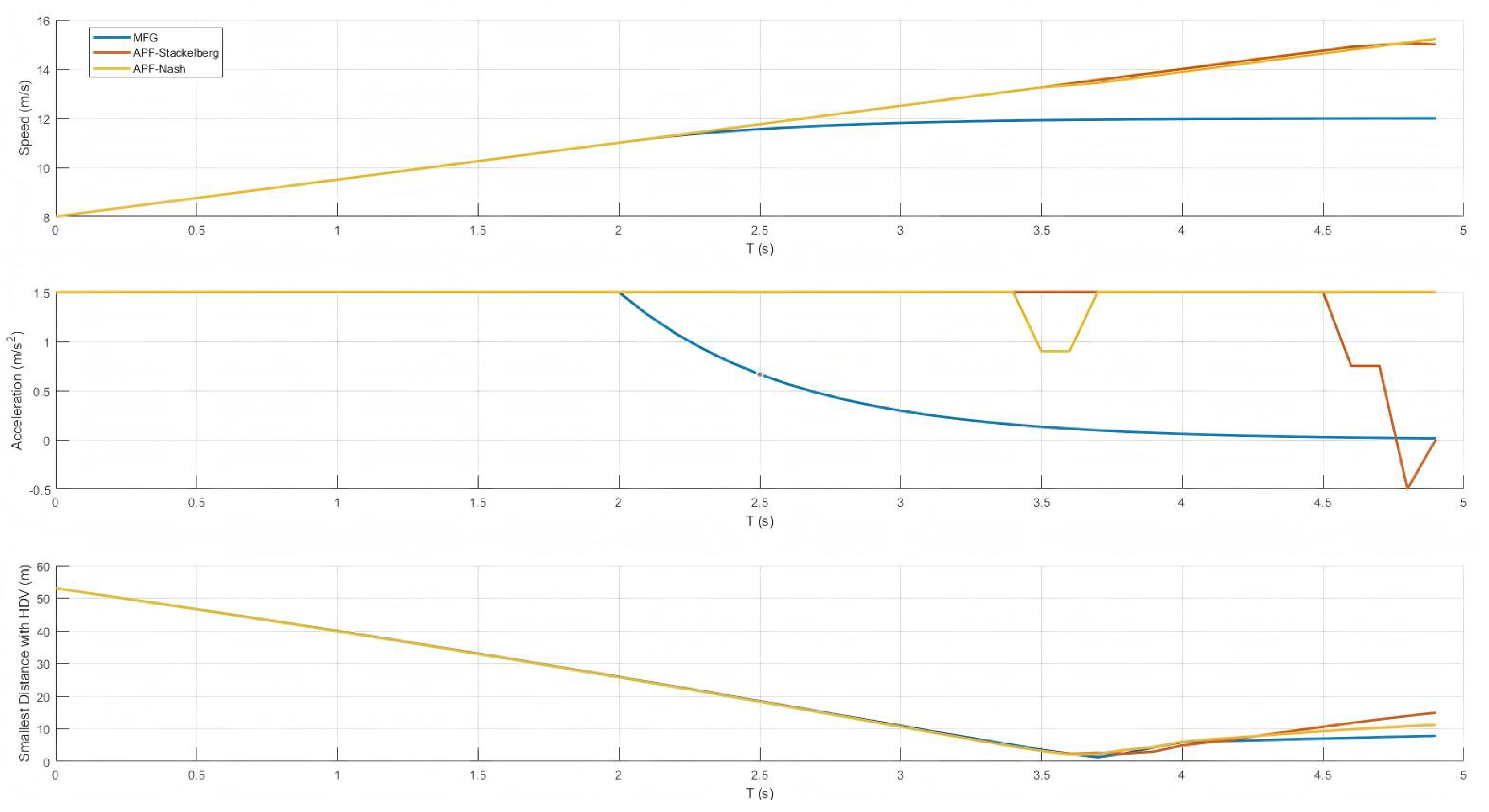
Figure 14 presents three subplots depicting the autonomous vehicle’s speed, acceleration, and its minimum distance to a follower human-driven vehicle over a five-second interval. The yellow curve represents our method, whereas the blue and orange curves correspond to the APF+Stackelberg and APF+Nash methods, respectively.
In the top subplot, our method shows a gradual increase in speed, resulting in smoother changes than the other two approaches. This reflects how the MFG scheme carefully balances forward progress and collision avoidance, avoiding abrupt accelerations. The middle subplot indicates that our acceleration profile remains comparatively stable, whereas the other methods may exhibit more sudden adjustments or even brief periods of zero or negative acceleration.
The bottom subplot depicts the smallest inter-vehicle distance between the autonomous vehicle and the follower HDV. While our method briefly attains a lower separation than the other approaches, this occurs at a point where the host vehicle is leading and the HDV behind it is assumed to maintain a fixed route rather than adapt for safety. In a real-world scenario, that HDV would naturally adjust its speed or lateral position to preserve a safer following distance. Consequently, the lower separation does not indicate a dangerous event but rather an artifact of our assumption that human-driven vehicles do not change their paths in response to the host vehicle’s maneuvers. These results highlight how our MFG-based control ensures a smooth speed profile while relying on follower vehicles to adjust their behavior in practical driving conditions.
6. Conclusion
In this paper, we have presented and evaluated an MFG framework integrated with an MPC-QP approach. Through multiple test scenarios and comparative studies against other potential field–based methods, we observed that our method maintains collision-free motion with smoother speed profiles and more stable lane-change or intersection maneuvers. In particular, the MFG component effectively captures the collective influence of surrounding vehicles, while the MPC formulation ensures real-time adaptability and efficient trajectory planning. These combined advantages enable our method to outperform benchmarks that lack explicit boundary constraints or rely on hierarchical or simultaneous equilibria without mean field modeling. Simulation results indicate that our method provides a promising, robust solution for multi-vehicle coordination, whether for AVs or HDVs in different driving scenarios. In future work, an MFG system could be designed for mixed traffic flows that include both HDVs and AVs, and various driving styles could be incorporated for further verification.
Author Contributions
Conceptualization, L.Z. and F.L.; methodology, X.W.; software, X.W.; validation, L.Z., F.L. and X.W.; formal analysis, X.W.; investigation, X.W. and Z.T.; resources, Z.T.; data curation, Z.T.; writing—original draft preparation, Z.T. and X.W.; writing—review and editing, Z.M. and Y.P.; visualization, F.Y.; supervision, C.Y.; project administration, F.Y.; funding acquisition, C.Y.. All authors have read and agreed to the published version of the manuscript.
Institutional Review Board Statement
Not applicable.
Informed Consent Statement
Not applicable.
Conflicts of Interest
The authors declare no conflicts of interest.
References
- Bai, X.; Peng, Y.; Li, D.; Liu, Z.; Mao, Z. Novel soft robotic finger model driven by electrohydrodynamic (EHD) pump. Journal of Zhejiang University-SCIENCE A 2024, 25, 596–604. [Google Scholar] [CrossRef]
- Peng, Y.; Sakai, Y.; Funabora, Y.; Yokoe, K.; Aoyama, T.; Doki, S. Funabot-Sleeve: A Wearable Device Employing McKibben Artificial Muscles for Haptic Sensation in the Forearm. IEEE Robotics and Automation Letters 2025, 10, 1944–1951. [Google Scholar] [CrossRef]
- Song, Z.; Liu, L.; Jia, F.; Luo, Y.; Jia, C.; Zhang, G.; Yang, L.; Wang, L. Robustness-aware 3d object detection in autonomous driving: A review and outlook. IEEE Transactions on Intelligent Transportation Systems 2024. [Google Scholar] [CrossRef]
- Lin, Z.; Zhang, Q.; Tian, Z.; Yu, P.; Lan, J. DPL-SLAM: Enhancing Dynamic Point-Line SLAM Through Dense Semantic Methods. IEEE Sensors Journal 2024, 24, 14596–14607. [Google Scholar] [CrossRef]
- Lin, Z.; Zhang, Q.; Tian, Z.; Yu, P.; Ye, Z.; Zhuang, H.; Lan, J. Slam2: Simultaneous localization and multimode mapping for indoor dynamic environments. Pattern Recognition 2025, 158, 111054. [Google Scholar] [CrossRef]
- Verma, H.; Siruvuri, S.V.; Budarapu, P. A machine learning-based image classification of silicon solar cells. International Journal of Hydromechatronics 2024, 7, 49–66. [Google Scholar] [CrossRef]
- Reda, M.; Onsy, A.; Haikal, A.Y.; Ghanbari, A. Path planning algorithms in the autonomous driving system: A comprehensive review. Robotics and Autonomous Systems 2024, 174, 104630. [Google Scholar] [CrossRef]
- Chen, L.; Wu, P.; Chitta, K.; Jaeger, B.; Geiger, A.; Li, H. End-to-end autonomous driving: Challenges and frontiers. IEEE Transactions on Pattern Analysis and Machine Intelligence 2024. [Google Scholar] [CrossRef]
- Teng, S.; Hu, X.; Deng, P.; Li, B.; Li, Y.; Ai, Y.; Yang, D.; Li, L.; Xuanyuan, Z.; Zhu, F.; et al. Motion planning for autonomous driving: The state of the art and future perspectives. IEEE Transactions on Intelligent Vehicles 2023, 8, 3692–3711. [Google Scholar] [CrossRef]
- Tsai, J.; Chang, Y.T.; Chen, Z.Y.; You, Z. Autonomous Driving Control for Passing Unsignalized Intersections Using the Semantic Segmentation Technique. Electronics 2024, 13, 484. [Google Scholar] [CrossRef]
- Barruffo, L.; Caiazzo, B.; Petrillo, A.; Santini, S. A GoA4 control architecture for the autonomous driving of high-speed trains over ETCS: Design and experimental validation. IEEE Transactions on Intelligent Transportation Systems 2024. [Google Scholar] [CrossRef]
- Mao, Z.; Peng, Y.; Hu, C.; Ding, R.; Yamada, Y.; Maeda, S. Soft computing-based predictive modeling of flexible electrohydrodynamic pumps. Biomimetic Intelligence and Robotics 2023, 3, 100114. [Google Scholar] [CrossRef]
- Mao, Z.; Kobayashi, R.; Nabae, H.; Suzumori, K. Multimodal Strain Sensing System for Shape Recognition of Tensegrity Structures by Combining Traditional Regression and Deep Learning Approaches. IEEE Robotics and Automation Letters 2024, 9, 10050–10056. [Google Scholar] [CrossRef]
- Lau, S.L.; Lim, J.; Chong, E.K.; Wang, X. Single-pixel image reconstruction based on block compressive sensing and convolutional neural network. International Journal of Hydromechatronics 2023, 6, 258–273. [Google Scholar] [CrossRef]
- Vishnu, C.; Abhinav, V.; Roy, D.; Mohan, C.K.; Babu, C.S. Improving multi-agent trajectory prediction using traffic states on interactive driving scenarios. IEEE Robotics and Automation Letters 2023, 8, 2708–2715. [Google Scholar] [CrossRef]
- Tan, H.; Lu, G.; Liu, M. Risk field model of driving and its application in modeling car-following behavior. IEEE Transactions on Intelligent Transportation Systems 2021, 23, 11605–11620. [Google Scholar] [CrossRef]
- Triharminto, H.H.; Wahyunggoro, O.; Adji, T.; Cahyadi, A.; Ardiyanto, I. A novel of repulsive function on artificial potential field for robot path planning. International Journal of Electrical and Computer Engineering 2016, 6, 3262. [Google Scholar] [CrossRef]
- Wu, P.; Gao, F.; Li, K. Humanlike decision and motion planning for expressway lane changing based on artificial potential field. IEEE Access 2022, 10, 4359–4373. [Google Scholar] [CrossRef]
- Lin, Z.; Tian, Z.; Zhang, Q.; Ye, Z.; Zhuang, H.; Lan, J. A conflicts-free, speed-lossless KAN-based reinforcement learning decision system for interactive driving in roundabouts. arXiv 2024, arXiv:2408.08242 2024. [Google Scholar]
- Tian, Z.; Zhao, D.; Lin, Z.; Zhao, W.; Flynn, D.; Jiang, Y.; Tian, D.; Zhang, Y.; Sun, Y. Efficient and Balanced Exploration-driven Decision Making for Autonomous Racing Using Local Information. IEEE Transactions on Intelligent Vehicles 2024, 1–17. [Google Scholar] [CrossRef]
- Tian, Z.; Zhao, D.; Lin, Z.; Flynn, D.; Zhao, W.; Tian, D. Balanced reward-inspired reinforcement learning for autonomous vehicle racing. In Proceedings of the 6th Annual Learning for Dynamics & Control Conference. PMLR; 2024; pp. 628–640. [Google Scholar]
- Tian, Z.; Lin, Z.; Zhao, D.; Zhao, W.; Flynn, D.; Ansari, S.; Wei, C. Evaluating Scenario-based Decision-making for Interactive Autonomous Driving Using Rational Criteria: A Survey. arXiv 2025, arXiv:2501.01886 2025. [Google Scholar]
- Zhen, T. Training-efficient deep reinforcement learning for safe autonomous driving. PhD thesis, University of Glasgow, 2025.
- Peng, Y.; Wang, Y.; Hu, F.; He, M.; Mao, Z.; Huang, X.; Ding, J. Predictive modeling of flexible EHD pumps using Kolmogorov–Arnold Networks. Biomimetic Intelligence and Robotics 2024, 4, 100184. [Google Scholar] [CrossRef]
- Boin, C.; Lei, L.; Yang, S.X. AVDDPG-Federated reinforcement learning applied to autonomous platoon control. Intelligence & Robotics 2022, 2. [Google Scholar] [CrossRef]
- Hassija, V.; Chamola, V.; Mahapatra, A.; Singal, A.; Goel, D.; Huang, K.; Scardapane, S.; Spinelli, I.; Mahmud, M.; Hussain, A. Interpreting black-box models: a review on explainable artificial intelligence. Cognitive Computation 2024, 16, 45–74. [Google Scholar] [CrossRef]
- Zhang, C.; Chen, J.; Li, J.; Peng, Y.; Mao, Z. Large language models for human–robot interaction: A review. Biomimetic Intelligence and Robotics 2023, 3, 100131. [Google Scholar] [CrossRef]
- Yang, D.; Cao, B.; Qu, S.; Lu, F.; Gu, S.; Chen, G. Retrieve-then-compare mitigates visual hallucination in multi-modal large language models. Intelligence & Robotics 2025, 5. [Google Scholar] [CrossRef]
- Huang, K.; Di, X.; Du, Q.; Chen, X. A game-theoretic framework for autonomous vehicles velocity control: Bridging microscopic differential games and macroscopic mean field games. arXiv 2019, arXiv:1903.06053 2019. [Google Scholar] [CrossRef]
- Chen, Y.; Veer, S.; Karkus, P.; Pavone, M. Interactive joint planning for autonomous vehicles. IEEE Robotics and Automation Letters 2023, 9, 987–994. [Google Scholar] [CrossRef]
- Liu, Y.; Wu, Y.; Li, W.; Cui, Y.; Wu, C.; Guo, G. Designing External Displays for Safe AV-HDV Interactions: Conveying Scenarios Decisions of Intelligent Cockpit. In Proceedings of the 2023 7th CAA International Conference on Vehicular Control and Intelligence (CVCI). IEEE; 2023; pp. 1–8. [Google Scholar]
- Liang, J.; Tan, C.; Yan, L.; Zhou, J.; Yin, G.; Yang, K. Interaction-Aware Trajectory Prediction for Safe Motion Planning in Autonomous Driving: A Transformer-Transfer Learning Approach. arXiv 2024, arXiv:2411.01475 2024. [Google Scholar]
- Gong, B.; Wang, F.; Lin, C.; Wu, D. Modeling HDV and CAV mixed traffic flow on a foggy two-lane highway with cellular automata and game theory model. Sustainability 2022, 14, 5899. [Google Scholar] [CrossRef]
- Yao, Z.; Deng, H.; Wu, Y.; Zhao, B.; Li, G.; Jiang, Y. Optimal lane-changing trajectory planning for autonomous vehicles considering energy consumption. Expert Systems with Applications 2023, 225, 120133. [Google Scholar] [CrossRef]
- Liu, Y.; Zhou, B.; Wang, X.; Li, L.; Cheng, S.; Chen, Z.; Li, G.; Zhang, L. Dynamic lane-changing trajectory planning for autonomous vehicles based on discrete global trajectory. IEEE Transactions on Intelligent Transportation Systems 2021, 23, 8513–8527. [Google Scholar] [CrossRef]
- Chai, R.; Tsourdos, A.; Chai, S.; Xia, Y.; Savvaris, A.; Chen, C.P. Multiphase overtaking maneuver planning for autonomous ground vehicles via a desensitized trajectory optimization approach. IEEE Transactions on Industrial Informatics 2022, 19, 74–87. [Google Scholar] [CrossRef]
- Palatti, J.; Aksjonov, A.; Alcan, G.; Kyrki, V. Planning for safe abortable overtaking maneuvers in autonomous driving. In Proceedings of the 2021 IEEE International Intelligent Transportation Systems Conference (ITSC). IEEE; 2021; pp. 508–514. [Google Scholar]
- Wang, Y.; Liu, Z.; Wang, J.; Du, B.; Qin, Y.; Liu, X.; Liu, L. A Stackelberg game-based approach to transaction optimization for distributed integrated energy system. Energy 2023, 283, 128475. [Google Scholar] [CrossRef]
- Ji, K.; Orsag, M.; Han, K. Lane-merging strategy for a self-driving car in dense traffic using the stackelberg game approach. Electronics 2021, 10, 894. [Google Scholar] [CrossRef]
- Hang, P.; Huang, C.; Hu, Z.; Xing, Y.; Lv, C. Decision making of connected automated vehicles at an unsignalized roundabout considering personalized driving behaviours. IEEE Transactions on Vehicular Technology 2021, 70, 4051–4064. [Google Scholar] [CrossRef]
- Kreps, D.M. Nash equilibrium. In Game theory; Springer, 1989; pp. 167–177.
- Hang, P.; Lv, C.; Huang, C.; Cai, J.; Hu, Z.; Xing, Y. An Integrated Framework of Decision Making and Motion Planning for Autonomous Vehicles Considering Social Behaviors. IEEE Transactions on Vehicular Technology 2020, 69, 14458–14469. [Google Scholar] [CrossRef]
- Tamaddoni, S.H.; Taheri, S.; Ahmadian, M. Optimal VSC design based on Nash strategy for differential 2-player games. In Proceedings of the 2009 IEEE International Conference on Systems, Man and Cybernetics. IEEE; 2009; pp. 2415–2420. [Google Scholar]
- Huang, K.; Chen, X.; Di, X.; Du, Q. Dynamic driving and routing games for autonomous vehicles on networks: A mean field game approach. Transportation Research Part C: Emerging Technologies 2021, 128, 103189. [Google Scholar]
- Mao, Z.; Hosoya, N.; Maeda, S. Flexible electrohydrodynamic fluid-driven valveless water pump via immiscible interface. Cyborg and Bionic Systems 2024, 5, 0091. [Google Scholar]
- Alawi, O.A.; Kamar, H.M.; Shawkat, M.M.; Al-Ani, M.M.; Mohammed, H.A.; Homod, R.Z.; Wahid, M.A. Artificial intelligence-based viscosity prediction of polyalphaolefin-boron nitride nanofluids. International Journal of Hydromechatronics 2024, 7, 89–112. [Google Scholar] [CrossRef]
- Peng, Y.; Yang, X.; Li, D.; Ma, Z.; Liu, Z.; Bai, X.; Mao, Z. Predicting flow status of a flexible rectifier using cognitive computing. Expert Systems with Applications 2025, 264, 125878. [Google Scholar] [CrossRef]
Figure 1.
Overview of the proposed MFG-MPC-QP framework.
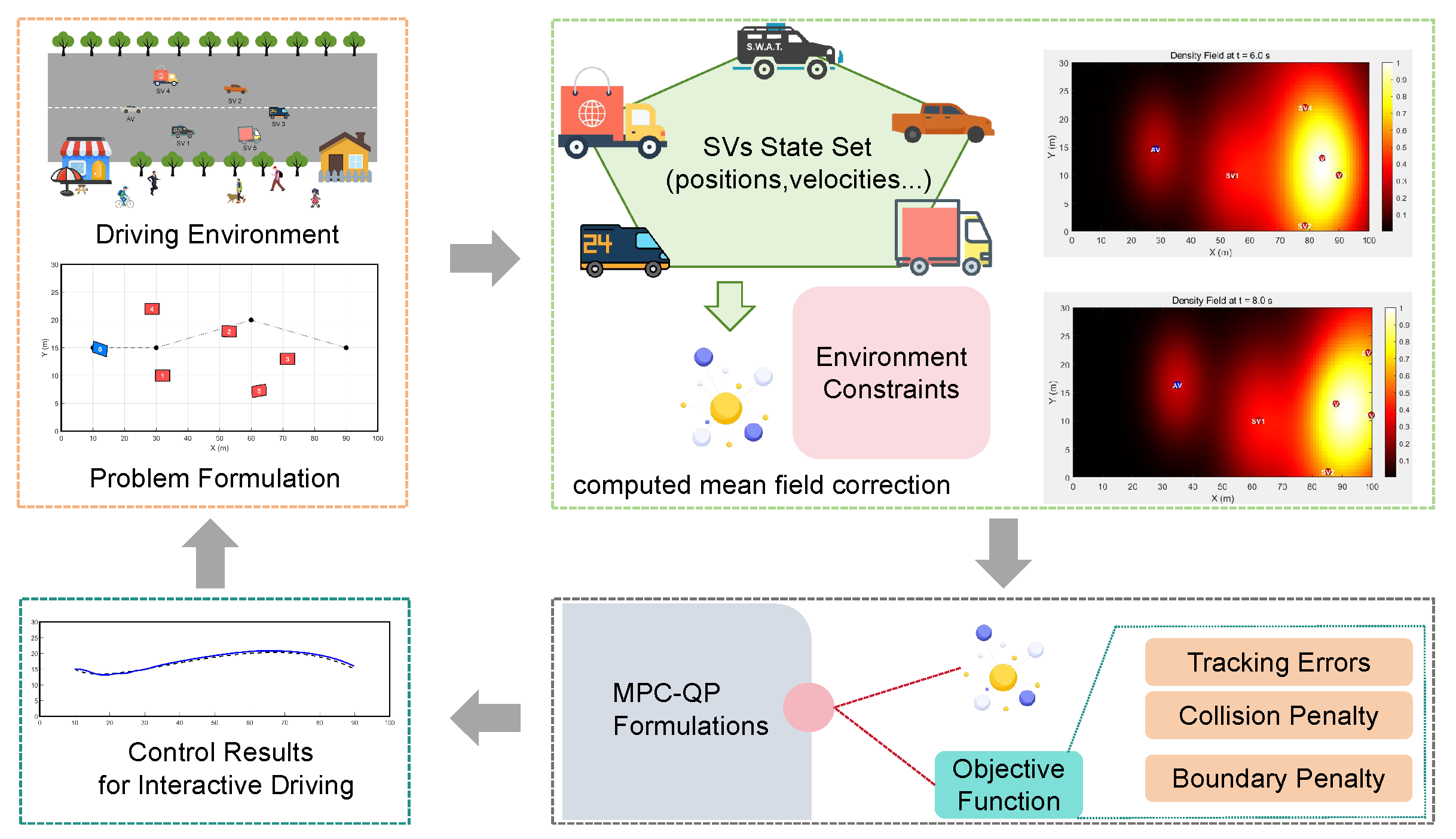
Figure 2.
Visualization of multi-vehicle traffic scenes and corresponding MFG-based density fields at four key times.
Figure 2.
Visualization of multi-vehicle traffic scenes and corresponding MFG-based density fields at four key times.
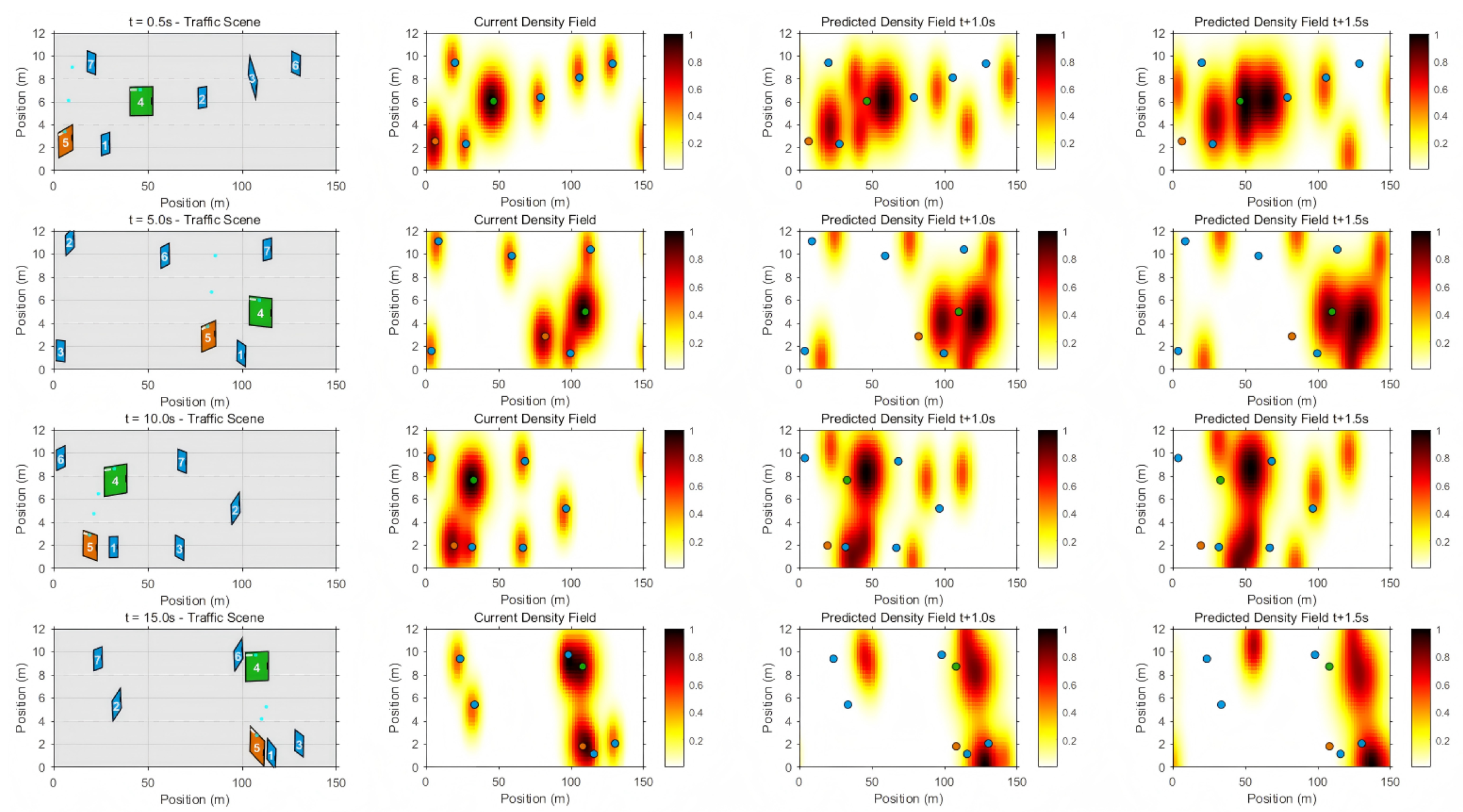
Figure 4.
Illustration of the first scenario. The host AV initiates interactive driving with surrounding HDVs in an irregular environment.
Figure 4.
Illustration of the first scenario. The host AV initiates interactive driving with surrounding HDVs in an irregular environment.
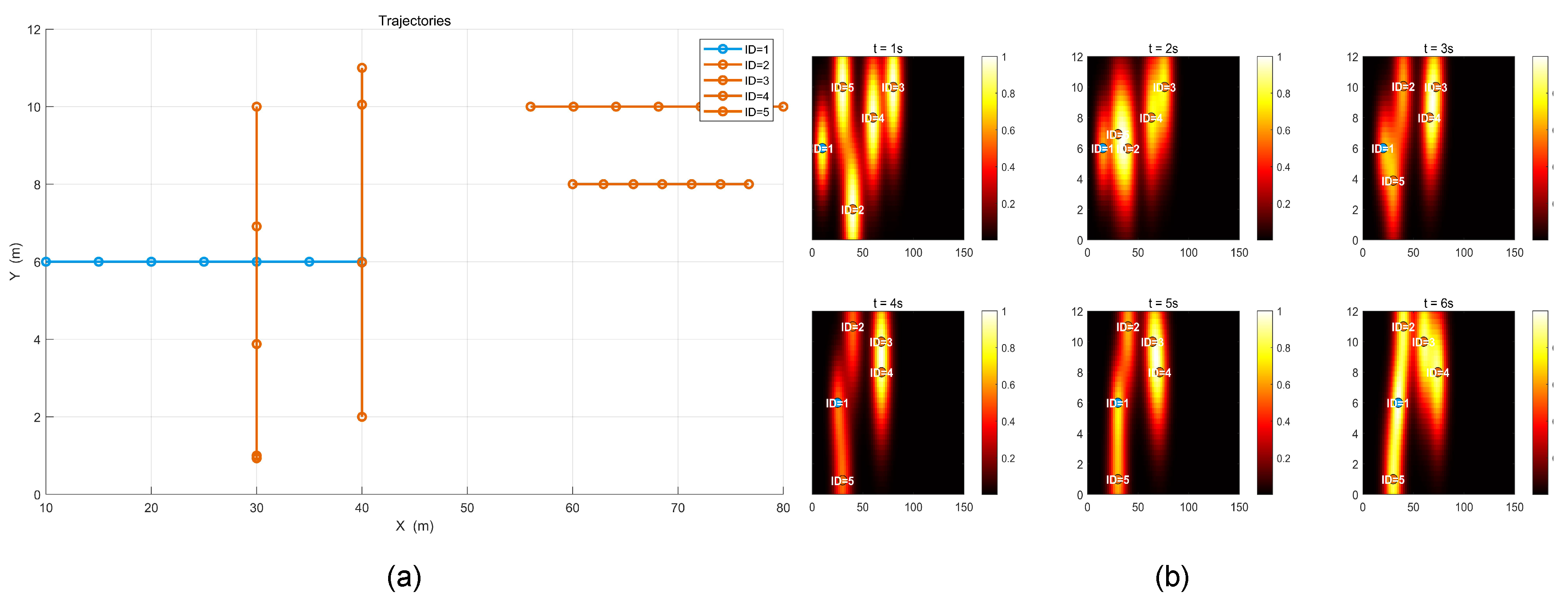
Figure 5.
(a) Visualization of vehicle paths over time in the x-y plane. The orange markers and lines correspond to a set of vehicles moving primarily along vertical lanes, while the blue markers and lines represent another vehicle traveling horizontally. These trajectories reflect how each vehicle’s position changes at each time step of the simulation. (b) Snapshots of the density field at several time instants (, , etc.), where warmer areas indicate higher density, and cooler areas show lower density. By examining these fields across multiple frames, one can observe how congested regions shift and expand as vehicles advance. Both subfigures are generated by the code output, illustrating the multi-vehicle environment and its evolution under collision-free conditions.
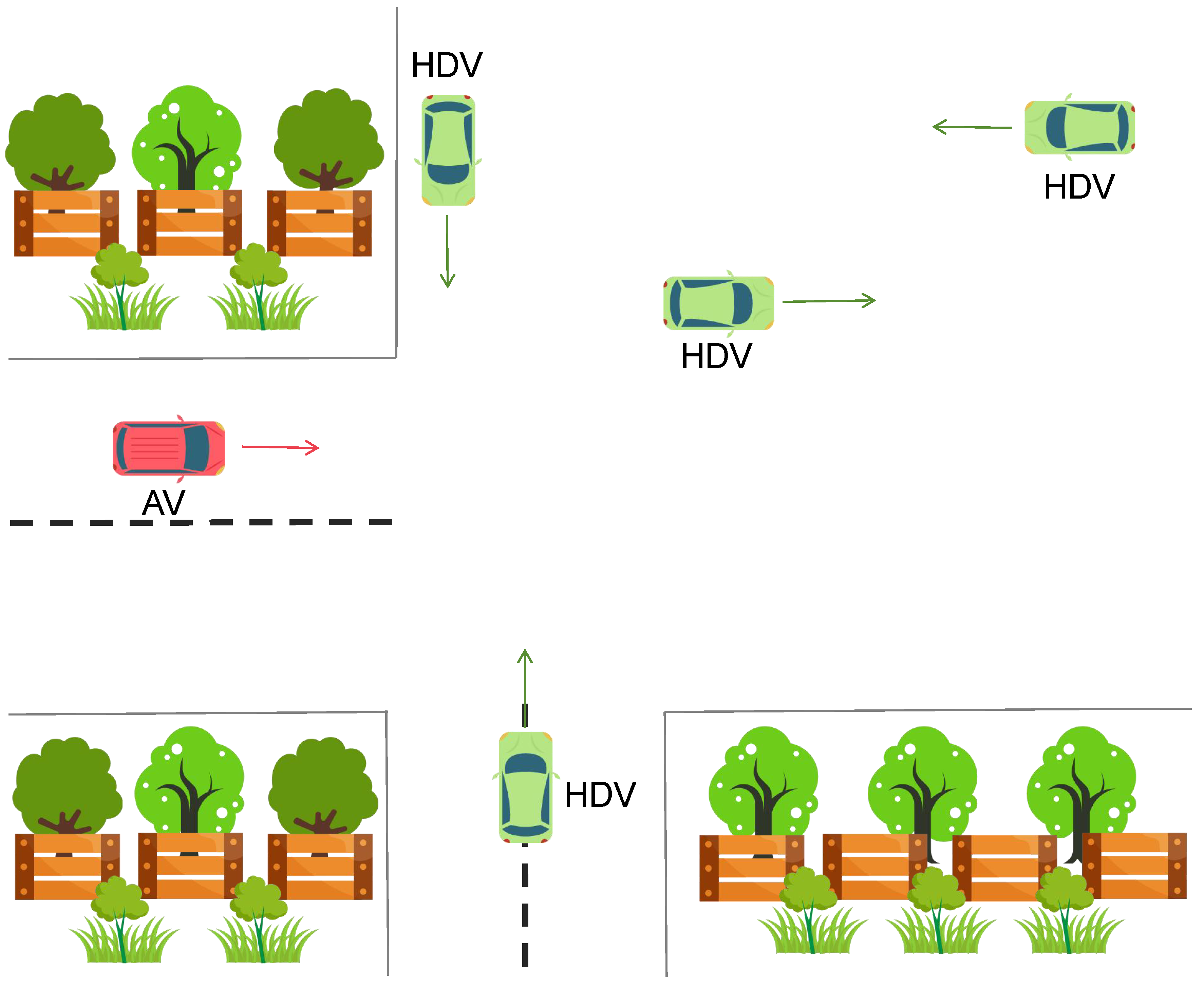
Figure 6.
Analysis of average speed and collisions over time.
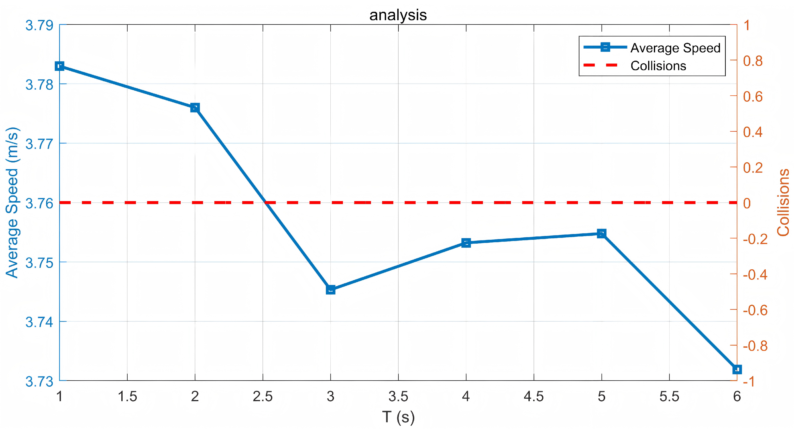
Figure 7.
Second scenario illustrating a multi-lane road, where the host vehicle aims to move from its current lane to the target lane.
Figure 7.
Second scenario illustrating a multi-lane road, where the host vehicle aims to move from its current lane to the target lane.
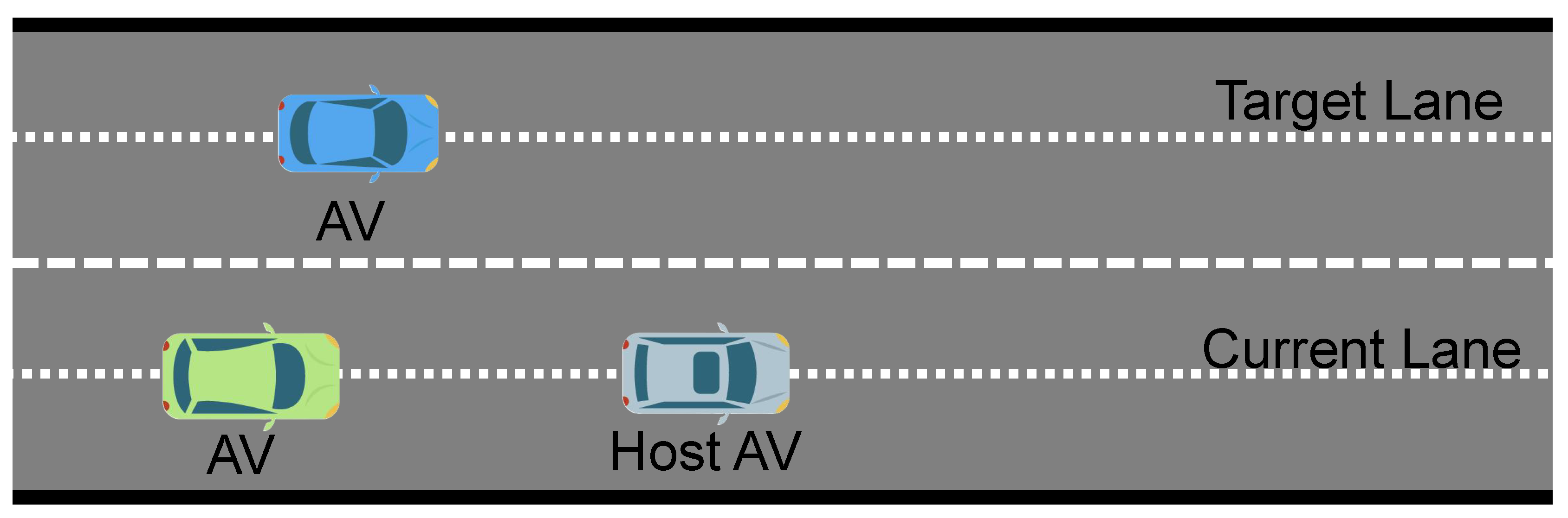
Figure 8.
Comparison of three vehicles’ trajectories using three different methods: MFG+MPC, APF+Stackelberg, and APF+Nash.
Figure 8.
Comparison of three vehicles’ trajectories using three different methods: MFG+MPC, APF+Stackelberg, and APF+Nash.
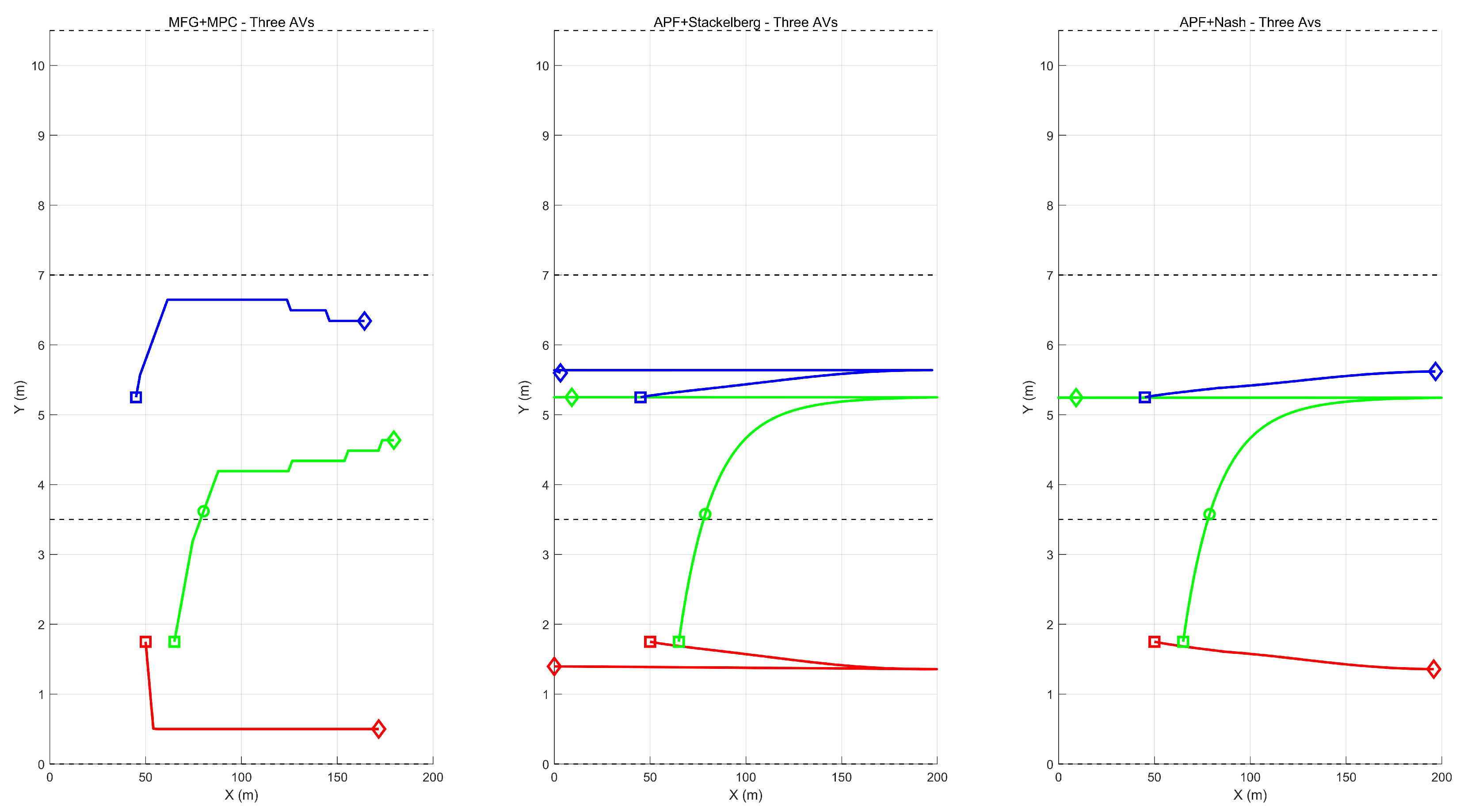
Figure 9.
Third test scenario with three lanes: an irrelevant lane, a current lane, and a target lane.
Figure 9.
Third test scenario with three lanes: an irrelevant lane, a current lane, and a target lane.
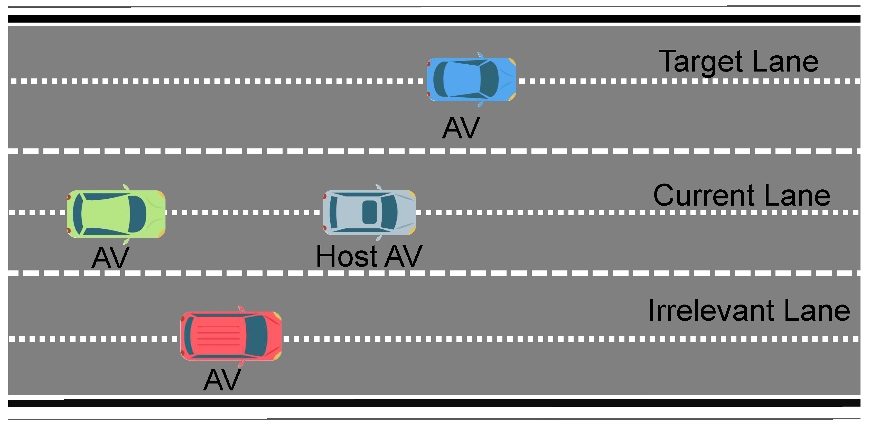
Figure 10.
Comparison of four AVs under three methods: MFG+MPC, APF+Stackelberg, and APF+Nash. Each color-coded path corresponds to a different AV.
Figure 10.
Comparison of four AVs under three methods: MFG+MPC, APF+Stackelberg, and APF+Nash. Each color-coded path corresponds to a different AV.
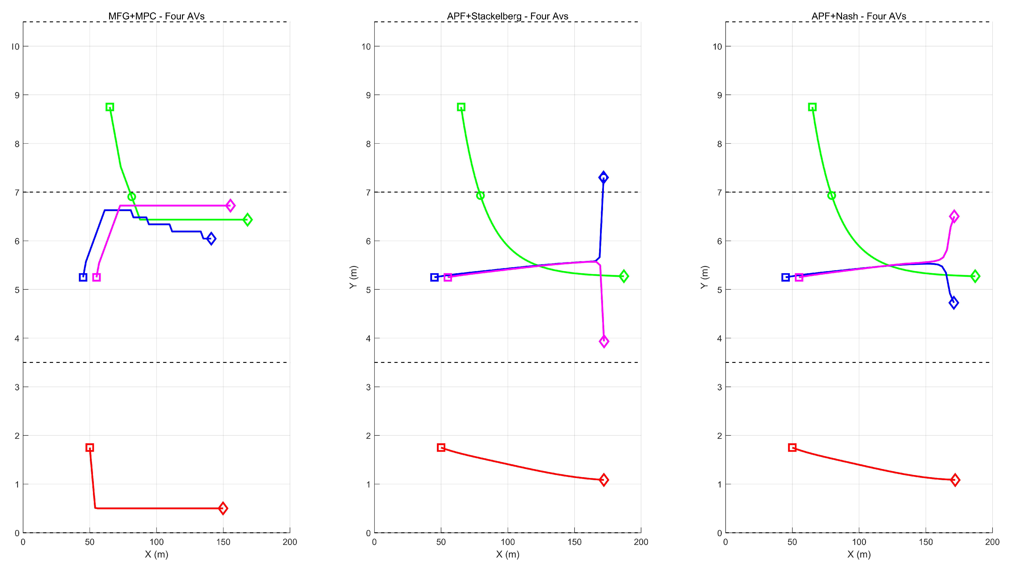
Figure 11.
Performance metrics across ten repeated runs under random longitudinal perturbations of up to for each AV. Each subplot compares three methods in two scenarios.
Figure 11.
Performance metrics across ten repeated runs under random longitudinal perturbations of up to for each AV. Each subplot compares three methods in two scenarios.
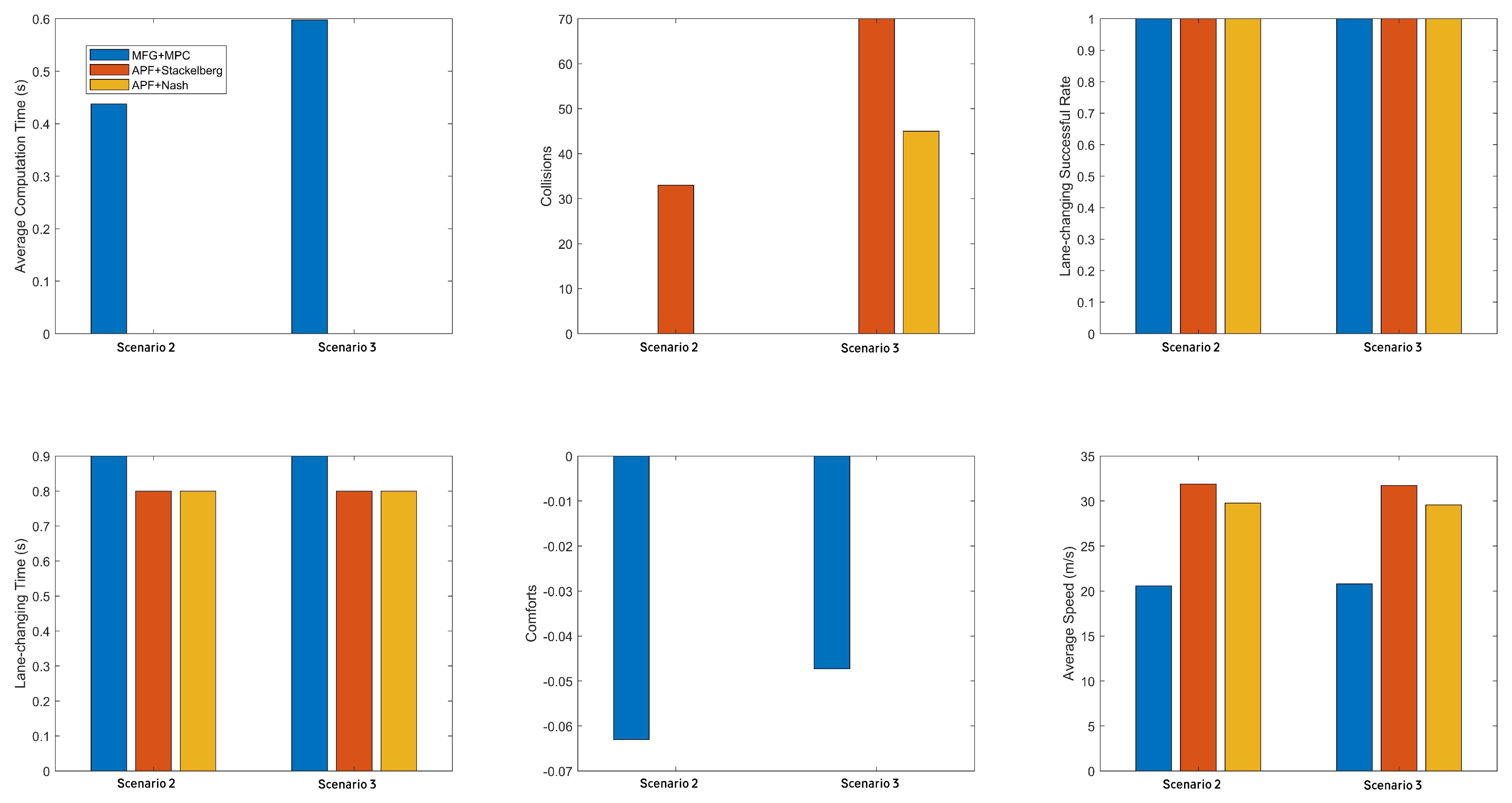
Figure 12.
Fourth test scenario with a multi-way intersection.
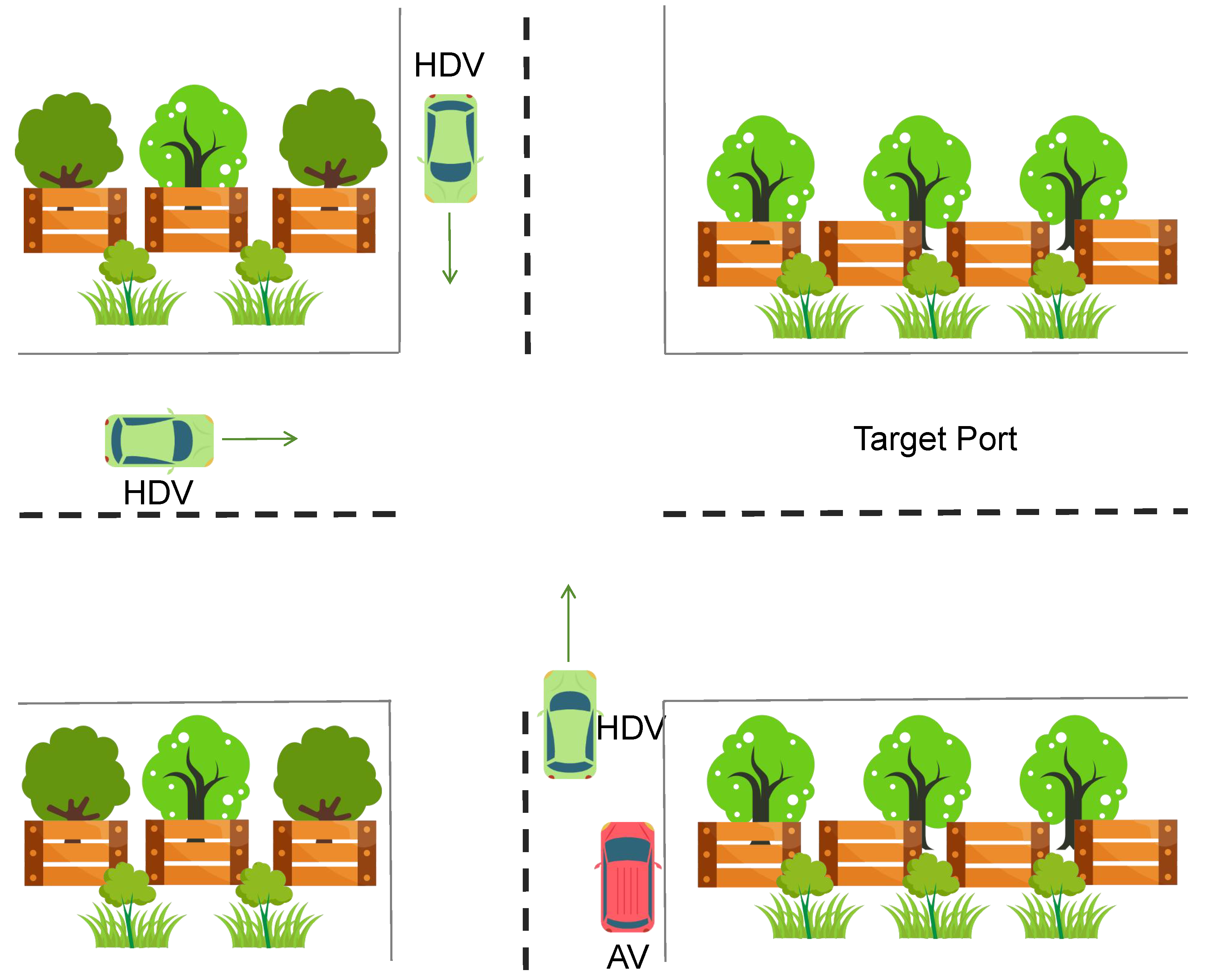
Figure 13.
Trajectories in a multi-way intersection under three methods: MFG, APF+Stackelberg, and APF+Nash.
Figure 13.
Trajectories in a multi-way intersection under three methods: MFG, APF+Stackelberg, and APF+Nash.
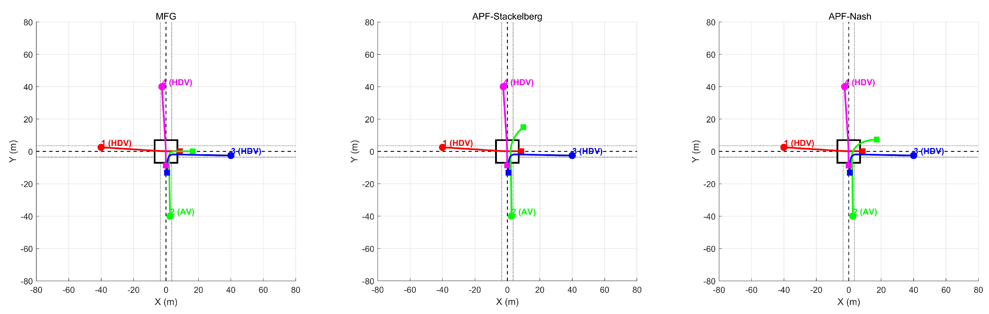
Figure 14.
Time histories of speed, acceleration, and smallest distance to a human-driven vehicle, comparing three methods: MFG, APF+Stackelberg, and APF+Nash.
Figure 14.
Time histories of speed, acceleration, and smallest distance to a human-driven vehicle, comparing three methods: MFG, APF+Stackelberg, and APF+Nash.
Disclaimer/Publisher’s Note: The statements, opinions and data contained in all publications are solely those of the individual author(s) and contributor(s) and not of MDPI and/or the editor(s). MDPI and/or the editor(s) disclaim responsibility for any injury to people or property resulting from any ideas, methods, instructions or products referred to in the content. |
© 2025 by the authors. Licensee MDPI, Basel, Switzerland. This article is an open access article distributed under the terms and conditions of the Creative Commons Attribution (CC BY) license (http://creativecommons.org/licenses/by/4.0/).
Copyright: This open access article is published under a Creative Commons CC BY 4.0 license, which permit the free download, distribution, and reuse, provided that the author and preprint are cited in any reuse.


