
Submitted:
22 April 2025
Posted:
23 April 2025
You are already at the latest version
Abstract
The quantum Rayleigh scattering of single photons, which is absent from the physical analyses of quantum optic experiments, destroys the mathematical concept of entangled photons. The quantum Rayleigh spontaneous and stimulated emissions provide physically meaningful interpretations for both polarization-based quantum correlations and beam splitter-based anti-correlations by means of groups of identical photons, commonly mistaken for one photon. These can overcome the quantum Rayleigh scattering of single photon in a dielectric medium. The random phases of spontaneously emitted photons play a critical role in obtaining visibility of unity with intensity correlations or number of photons. It is the ratio of physically present photon numbers that determine the visibility rather than a superposition of randomly detected numbers of photons. The intrinsic field of a photon is the same regardless of the optical source. The evolution of the photonic properties of each input of a pure quantum dynamic and coherent number state is described by the Ehrenfest theorem breaking away from the Copenhagen approach of time- and space-independent inputs of mixed density matrices which appear to lead to physically counter-intuitive interpretations.
Keywords:
intrinsic field of photons
; quantum Rayleigh scattering
; quantum correlations
1. Introduction
The much anticipated and long-promised revolution of quantum computer operations is predicated on strong quantum correlations of measured properties of particles or photons to generate statistical data sets. For instance, polarization-entangled single photons have been held up as a practical way of performing quantum operations. Equally, the indistinguishability of single photons is assessed by means of the Hong-Ou-Mandel (HOM) anti-correlation apparently generated through a beam splitter.
Nevertheless, as recently pointed out in background briefing articles [1,2], a practical quantum computer is many years away as heavy investment of resources has, so far, failed to make significant headway in solving many and varied obstacles brought about by physical and technical problems.
Therefore, a physical scrutiny of quantum correlations would be of practical and immediate physical interest. Relying on the concept of pairs of entangled photons, the design of quantum logic circuits would be based on statistical outputs of density matrices of mixed states of the photonic systems. However, in quantum physics these time- and space-independent density matrices cannot explain the propagation of photons through dielectric media and the photon-dipole interactions as they deal with averaged outputs as opposed to time- and space-dependent instantaneous and sequential output values which are later averaged. A brief outline of this latter approach which eliminates counter-intuitive explanations, can be found in Appendix A.
It is a common practice in the field of quantum optics to reiterate without any critical consideration the narrative of having the probing or measurement of one entangled-photon influence the measured properties of the other paired photon. However, the criteria which are used to assess such outcomes are rather indirect through the Bell-type inequalities, of which the Clauser-Horne-Shimony-Holt (CHSH) inequality is the most popular and used in all sorts of experiments. Subject to device independence “…the violation of Bell inequalities can be seen as a detector of entanglement that is robust to any experimental imperfection: as long as a violation is observed, we have the guarantee, independently of any implementation details, that the two systems are entangled. This remark is important: since entanglement is at the basis of many protocols in quantum information, and, in particular, quantum cryptographic protocols, it opens the way to device-independent tests of their performance. “ [3] (p. 423).
Nevertheless, experimental results obtained with independent photons violate Bell-type inequalities [4,5]. Additionally, for maximal values of unity correlations, the Bell parameter of eq. (4) in ref. [3] would actually vanish as and according to the expectation values [3, p. 422] of , for detection settings and of the polarization states for coincident detections. Thus, , failing to violate the CHSH inequality despite involving the strongest quantum correlations. This fact should have rung alarm bells about the irrelevance of the Bell-type inequalities as an indicator of strong correlations between the same order elements of two sequences.
A recently published article [6] reported results of the speed of “spooky action at a distance” (SAD). We quote: “The experiment is based on the idea that, if the speed of SAD is finite, and the detection events (A and B) are simultaneous in the privileged frame, the communication between two events does not arrive on time and Bell violation is not observed.” A similar experiment had been reported previously in ref. [7] with a different type of correlation measurements. The outcomes of these two experiments are explained with physically meaningful processes in this article.
Despite significant technological developments in the design and fabrication of devices and components used in experiments aiming to prove the existence of quantum nonlocality phenomena based on single and entangled- photons, the detection rates of such alleged phenomena are very low [8,9], which fact was completely ignored in ref. [10]. Additionally, the analyses of those experimental outcomes have repeatedly ignored or omitted many aspects of optical physics and mathematical analysis, such as:
1. Published experimental results in other journals than Physical Review Letters, have reported quantum-strong correlations with independent photons [4,5] based on polarization measurements. These results are consistent with the expansion of the Pauli vector correlation operator [3; p. 422] leading to an identity operator multiplied by the correlation function, i.e., the operator can be can reduced to [11]; (Eq. (A6)) to:
2. A single photon is deflected from a straight-line propagation in a dielectric medium by the quantum Rayleigh scattering of single photons [13]. Groups of identical photons can propagate in a straight-line through quantum stimulated Rayleigh emission (QRStE) [14,15]. The spontaneously emitted photons in the nonlinear crystal undergo parametric amplification forming a group of identical photons which can overcome the quantum Rayleigh scattering through quantum Rayleigh stimulated emission [14,15]. Similarly, the effect of QRStE plays a critical role in creating groups of identical photons in a commonly used dielectric beam splitter – from the scattered single photons – as explained in ref. [15]. This physical aspect should have been taken into consideration over the last four decades.
In light of these two major aspects which are missing from the analytic interpretations of experiments purporting to prove the phenomenon of quantum nonlocality, this article will address in Section 2 the two-step sequential detections of the entangled pair of photons for quantum correlations between photonic polarization states evaluated with the von Neumann postulate of projective measurements to explain the results of refs. [4,5,6,7,8,9]. These limited correlations will be compared to the those between independent photons, which indicate the possibility of very strong correlation between the polarization filter states.
Correlations between same order pairs of photons vs correlation between state vectors are specifically differentiated in Section 3 in the context of experimental outcomes. Equally, the shortcomings of Bell inequalities are outlined.
Based on the photonic fields of the dynamic and coherent fields, the unavoidable parametric amplification forming groups of identical photons or monochromatic pulses are presented in Section 4. Intensity correlations based on the intrinsic fields of photons may deliver 100% visibility of either the product of two fringe photocurrents or the discrete counting of detected low number of photons as a result of the random phases of amplified spontaneous emission.
2. Quantum Correlation of Polarization States
Quantum nonlocality based on correlations between single and entangled photons would have the first measurement influence the second measurement. This phenomenon should generate outcome correlation between remote detection stations, which would exceed ‘classical’ correlations.
In this Section, two consecutive projective measurements are analysed for an entangled state of single photons which will identify criteria for a claim of nonlocality. Equally, a second analysis of independent photons will reveal stronger remote correlations.
2.1. Quantum Correlations Based on the Von Neumann Projection Postulate
If only one photon reaches each of the two separate detecting stations, only one of the two orthogonal polarization channels will be triggered. Thus, four one-to-one correlation data sets will be recorded as the measurement ensembles build up [6].
As an example of the quantum expectation value of correlation between two detection settings – one at each location – we consider the projective measurement at location B involving the operator
acting on the initial state
Next, a first detection takes place at location A involving the projective operator , which results in the intermediary state for the projective amplitudes and , so that the reduced or collapsed wave function becomes:
Based on the normalized state , the probability of detection at location B following a detection at location A becomes in this case, for a projective measurement:
This result which can be found in [16]; [Sec.19.5] implies that for, regardless of the values of , the local probability of detection could peak at unity. This theoretical outcome is easily testable experimentally for direct evidence of a quantum nonlocal effect influencing the second measurement after the wave function collapse. But this has never been done either because of the quantum Rayleigh scattering of a single-photon and/or the non-existence of such a nonlocal effect. The product of the local probabilities of eqs. (4) and (5) equals the expression of the joint probability for simultaneous detections at both locations A and B, that is:
The possibility of factorizing the quantum probability for joint events as in (6a) is identical to the classical case of conditional joint probabilities with the second local probability being conditioned on a first detection. This strong similarity between the classical and quantum joint probabilities renders the local condition of separability [3,16] irrelevant for the derivation of Bell inequalities.
As eqs. (4-6) indicate, the correlation between the two stations is the same regardless of whether the two separate measurements are sequential or simultaneous, thereby contradicting the assumption of refs. [6,7] that the fringe formation should vanish for simultaneous measurements. This is also contradicted by the fact that the correlation takes place between the detecting directions as expressed in eq. (1).
However, as local measurements at location B result in a difference between = 1/2 and , experimental proof, or otherwise, of any quantum nonlocal effects can be verified by carrying out two ensembles of measurements, one with a prior detection at location A and the second one without such a detection. Additionally, by switching on and off the measurement at location A, a signal would be detected at location B between zero and non-zero probabilities, by simply coordinating the two filters’ angles to be equal for the zero probability of joint detections.
The use of a global quantum state which is time- and space-independent for the description of a time-dependent source output has led in many cases to physically impossible conclusions which were, nonetheless, taken as the “miracles” of quantum optics and quantum mechanics. In other words, even though information about the quantum system can be obtained from each individual measurement, the predictions of expected values of dynamic variables are based on global quantum states which discard a great deal of information.
2.2. Quantum Correlations of Independent Photons
Quantum correlations are evaluated as the expectation values of a product of operators [3,16]. For the projective operators corresponding to the polarization filters with one detection setting at each of the two locations A and B, respectively, the probability of coincident detections has the form, cf. [3, eq. 13]:
Experimentally, with , for no-detection or a recorded detection of the mth event, respectively, the probability of coincident detections is calculated from the normalized sum of products of overlapping terms, i.e., . Depending on the sequantial orders, this can exceed the product of local probabilities of detections . The probability of coincident detections identifies the fraction of simultaneous detections at the level of each quantum event but the quantum formalism cannot provide the sequential orders of the detected events. This discrepancy is part of the disconnect between theory and measurement as the former delivers only a quantum expectation value, the latter identifies coincidences between two mth order elements.
For the basis states of the shared measurement Hilbert space, the projective amplitudes are , , and . The correlation function of magnitude between filter polarization states and for independent states of photons becomes:
3. Quantum State Correlations Versus Photon-to-Photon Correlations
Two types of correlations can be identified in the context of quantum correlations: the state-to state correlation and the sequential element-to element correlations. The former is found in the theory of quantum correlation while the latter is used to calculate the experimental correlations. As a consequence, a disconnect between experimental outcomes and theory emerges.
3.1. State-to-State Correlations
The quantum correlation function for detecting one photon at location A and its pair-photon at location B, is defined in terms of four probabilities between two orthonormal detection-settings at each of the two locations A and B, for eigenvalues , respectively, of local settings , and leading to the linear combination of probabilities [16,17]:
By inserting corresponding values of from eq. (6b) into eq. (9) and comparing eqs. (1) and (9), we obtain for the angles on the Poincaré sphere:
For the CHSH inequality [17], the correlation probability is with the number of coincident counts of photons and the number of all coincident detections for all four settings . However, this normalization is mathematical because the physical number of initiated photon-pairs is very much larger as photons are lost between the source and the photodetectors, for various reasons, thereby throwing doubt about the real statistics. This normalization makes a violation of the CHSC impossible as . This is the case of ref. [6] with its Figure 1 showing a very low success rate of detection of only 150 coincidences over 5s integration time despite 1 million events per second.
The Clauser-Horne (CH) inequality has arbitrary values for the two measurement settings, i.e., as well as are set separately. The CH inequality also contains correlations between ‘1’s and ‘0’s, so that, in terms of binary-valued probabilities and similar forms, [8,9], the inequality is written as:
In order to prove the existence of a quantum nonlocality effect at the level of a single event involving a pair of entangled photons, there is no need for Bell inequalities. Only one setting at each detection station is necessary, e.g., the term of eq. (11), for proving or disproving the concept of quantum non-locality. But as already mentioned, the maximal value measured in refs. [8,9] is a mere 2x10⁻⁴ (or 0.0002), which does not exceed noise contributions.
3.2. Sequential Element-to-Element Correlations
As pointed out in ref. [3], in typical experiments of correlated outputs, the results of the joint probability of simultaneous or synchronized detections of two sequential ensembles of binary values, do not equal the product of the two separate probabilities of detection at locations A and B for outcome and corresponding to local settings and , respectively, that is: where are assigned binary values for no-detection or detection of an event, respectively.
In an attempt to explain experimental outcomes obtained with quantum events, it was suggested to convert into an equality of local probabilities [3]:
From an experimental perspective, the correlation probability of simultaneous detections is evaluated from a third sequential distribution calculated as the temporal vector or dot product of the two initial and separately measured, sequences and leading to of Section 2.1,
where is the number of detection windows or initial number of experimental runs. The rotation angles of the local polarization filters are . For any ensemble of measurements, the values of the correlation or conditional joint probability will depend on the sequential orders of the two separate ensembles at locations A and B. Therefore, as the quantum formalism does not provide any information about those sequential orders, any artificial boundary such as Bell-inequalities is physically meaningless, because for the same values of the local probabilities the higher values of exceed the arbitrary upper limit of eq. (12) rendering any further derivation physically irrelevant as it is intentionally limited in value. Bell inequalities can be easily violated with independent photons [4,5,12].
As explained in the Introduction section, for maximal values of unity correlation the Bell parameter vanishes , failing to violate the CHSH inequality despite involving the strongest quantum correlations. In fact, only correlation values of around 0.7, with sign adjustments, violate Bell inequalities, which is identical to the case of ‘classical’ correlations.
The 2015 landmark experiments [8,9] reported a very low probability of coincident detections of a mere 0.0002 (2x10--4) with one setting at each of the two stations, the overall outcomes being fitted with highly non-entangled states of photons, thereby disproving any claim of quantum nonlocality despite the common view [10].
The effect of quantum nonlocality is meant to synchronize the detections recorded at the two locations A and B for polarization-entangled states of photons. In the caption to Figure 1 of [10], on its second page, one reads: “…if both polarizers are aligned along the same direction (a=b), then the results of A and B will be either (+1; +1) or (-1; -1) but never (+1; -1) or (-1; +1.); this is a total correlation as can be determined by measuring the four rates with the fourfold detection circuit.” Yet, the quantum correlation is supposed to take place at the level of each pair of entangled photons rather than between averaged values of the two distributions; but such an outcome has never been reported, which fact was ignored in ref. [10].
Nowhere in the professional literature has the following question been addressed: How can a single photon avoid photon-dipole interactions of absorption and re-emission given the Avogadro number of 6.02214076 × 10²³ atoms per mole? Otherwise, no synchronized detections of the initial pair of photons is possible, ruling out any effect of quantum nonlocality. A few dielectric components are used in the experimental setups of ref. [6,7] such as: a dichroic beam splitter acting as a spectral filter (SF), polarization waveplates, and the medium of the parametric source itself. Also, a “cw laser source” is used, so that the spontaneously emitted photons are randomly distributed in time. Groups of identical photons are formed through parametric amplification of spontaneously emitted paired photons as explained previously [14,15] (see Appendix A), and they will generate at location B the interference pattern as follows in Section 4.
4. Groups of Identical Photons Mistaken for Single Photons
The conventional interpretations of experimental results of quantum correlations which are, allegedly, based on single and entangled photons originated in the 1986s with the appearance of optical sources employing the spontaneous, parametric down-conversion of pump photons [18] This section outlines the physical contradictions of the Mandel approach [18] and presents analyses based on time-varying pure states that eliminate the quantum miracles listed in the literature. These analyses take into consideration the roles played by the optical devices in the generation, propagation, processing and detection of photons.
4.1. A Brief Description of Dynamic and Coherent Number States
Let us follow the propagation of a spontaneously emitted photon in the optically nonlinear process of spontaneous parametric down-conversion (SPDC) of a pump photon. This photon, and similarly its parametric pair-photon, can be emitted in any direction compatible with the emission pattern of an electric dipole as the oscillating electron can move about the equilibrium position to absorb any residual momentum. When these two photons are launched in the same direction as the propagating pump, even in the absence of phase-matching, these photons can be amplified [15] as their phases vary rapidly, through the phase-pulling effect, leading to the optimal relative phase for maximal amplification – sees Appendix A. Thus, both the signal and idler beams generate groups of identical photons which are described mathematically by means of the mixed time-frequency representation [14], i.e., a time-varying number of monochromatic photons whose spatially limited field profiles interact with local electric dipoles giving rise to quantum Rayleigh spontaneous and stimulated emissions [13,14]. When such a group of monochromatic photons crosses a spectral filter, the internal back-and-forth partial reflections spread the group temporally which is the equivalent of and mistaken for the narrowing of a Fourier spectrum.
These two physical processes of parametric amplification and time-stretching, and the quantum Rayleigh scattering of single photons [13] are missing from the conventional interpretation of quantum optics, which leads to the need for ‘counter-intuitive’ interpretations of quantum nonlocality. Groups of photons generated by parametric amplification of spontaneous emission in a nonlinear crystal – see Appendix A – will undergo temporal stretching, splitting and delays as they propagate through spectral filters, Bragg gratings, beam splitters or other devices [6,7,14,15], so that for a continuous pumping of the nonlinear crystal a quasi-continuum of photons will be present in the experimental system at any given time. A combination of a low level of amplification of a spontaneously emitted photon into a group of identical photons along with propagation losses sustained in dielectric media, and with the reflective dispersion of photons and the imperfect quantum efficiency of photodetectors, will result in the effective number of photons being low enough not to trigger a detection below a threshold. This threshold is possibly related to the background noise radiation and the limited number of electrons available for photon-dipole interactions in the detector. Thus, what seemed to be a “classical” case turns into a quantum regime-like detection with photon number fluctuations and randomly generated phases determining the instantaneous ratio of interference-detected photons to the sum of input numbers of photons. The instantaneously measured ratio follows the conventional interference pattern [14] of
Following the results of [14,15], we identify dynamic and coherent number states and recall the non-Hermicity of the field creation and annihilation operators [16]. We find for the number states that , which provides the complex field of the amplitude, for the time-dependent evolutions of photonic beam fronts [14] associated with the wave function . Similarly, the expectation values of the instantaneous number of photons carried by a mode, the optical field magnitude and its phase are readily evaluated with the state , for the respective photonic operators [14]. The evolution of the complex amplitude is determined by means of the Ehrenfest theorem for the expectation value [14]. Additionally, the longitudinal and lateral distributions of one photon are calculated from differential equations derived from a combination of the Maxwell equations and the quantum expectation values. These profiles are given in closed form by [14]:
4.2. Examples of Correlations
A few examples of experimental results which are explained by means of the intrinsic field of photons are presented in this subsection.
Example 1 – The experimental results of ref. [6] are easily explained by taking into consideration the unavoidable parametric amplification of spontaneously emitted photons [12,14,15] – see Appendix A for a brief summary.
With multiple photons propagating in both input orthogonal states of polarization H and V, one can control the output intensity through interference of the intrinsic fields [14] of groups of identical photons coupled onto the filter’s polarization state of rotation angle .
A group of identical photons generated through amplification in the original crystal source is carried by a linearly polarized radiation mode. These photons couple into the local eigenmodes H and V of polarization-rotating waveplates. As the two local eigenmodes H and V reach the polarization filter at location A or B, their photons are projected onto the polarisation analyser’s orientation of angle . As a result, a rotation dependent interference pattern is created with the photo-current being proportional to the instantaneous number of photons .
At location B, the detector’s output intensity for fluctuating numbers of photons and the expectation number of the interference between the projected pure states, take the forms [14,15]:
A basic principle of scientific methodology for reproducibility of outcomes states that identical systems operated under identical conditions will yield identical distributions of output data. For ref. [6] the orthogonal inputs are (. The rotational invariance of the detection filters aligned with the incoming photon’s polarization leads to an offset angle difference of for the initially maximal and identical, superposed fringes of interference for correlation values. These settings and photocurrents are created locally and the curves of Figure 1 of [6] are determined locally at station B, while the setting at location A is kept constant.
Experimentally, correlations of detected photons are probed by the product of the discretized photocurrents [14] by using eq. (15b), so that:
Example 2 - An earlier experiment [7] employed an intensity Franson interferometer [18] comparing the outcomes of two separate 1 x 1 unbalanced Mach-Zehnder interferometers (MZI). The outcomes of this configuration can easily be explained in terms of the two separate and synchronized interference patterns as in eq. (16). Instead of a polarization rotation, a locally controlled phase-shift brings about the interference pattern of apparent coincident detections which have, as before, a very low success rate using a continuous-wave laser pump. The interference is local because it involves only the amplified spontaneous emission of one output mode, i.e, signal or idler of the parametric source, reaching the local detector in the form of two sub-groups of photons after the original group passed through a spectral filter that spreads out, or stretches, the input group of photons by internal back and forth partial reflections.
With the SPDC signal and idler beams being directed separately to location A and location B, respectively, a group of photons is split by internal partial reflections into two parts 1 and 2 in the spectral filter with the second sub-group being delayed in time. As each sub-group reaches the unbalanced MZI, a fraction of the first partial group runs along the longer arm of the MZI and interferes with the fraction of the second partial group that followed the shorter arm of the MZI. As both partial groups split from the same original group through temporal delays in a spectral filter, they share the same original spontaneous phase . Upon reaching the same photodetector after crossing an MZI, they create interference fringes through an external phase modulation in one of the arms. At the other detector, the level of detection is kept constant – possibly maximized – being triggered by a randomly detected photon. Thus, the correlation takes the form
Example 3 -The case of the Hong-Ou-Mandel (HOM) dip is illustrated in Figure 1 and was explained in ref. [14] by recalling that the two outputs share the same random phase-difference with and . Thus, in eq. (17a), . The internal reflection from a higher-index medium inside a cubic beam splitter induces a phase-shift . Using the identity , in eq. (17) the average over the random phases evenly distributed in the range of results in term vanishing while the first term of negative unity should be counted twice because the phases can interchange values for the same outcome. Alternatively, the contributions in eq. (17) of the terms add up to zero by integrating over the phase interval of while for , the product term of eq. (17) becomes and its contributions in the range cover two periods of rad with two positive values of 1/2 adding up to negative unity. It should be emphasized that the instantaneous values of the interference terms are measured to build up an ensemble of measurements, and the statistically averaged value is calculated at the end of the data acquisition through normalization with the number of initiated events, whether recorded or not by the detectors. The average does not involve a phase integration as suggested in ref. [20] where the mixed quantum state of the time-independent coherent state was employed. The shortcomings of this approach [20] are listed in the discussion Section 5.
The visibility coefficient (with j = A or B), contains two factors. The ratio of photon numbers will determine the visibility
As in the previous Example 2, spectral filters will reduce the initial number of photons in each group of identical photons exiting the SPDC source while discretely spreading the initial group by back and forth partial reflections. This requires a minimum number of initial photons so that enough of the dwindling group will survive the propagation to the photodetector. This is consistent with the experimental correlations with uncorrelated photons [21].
The visibility higher than 0.5 reported by ref. [22] was obtained with fluctuating pulses of multiple photons attenuated, allegedly, to the level of one photon. Yet, no explanation was provided therein about the quantum Rayleigh scattering of single photons.
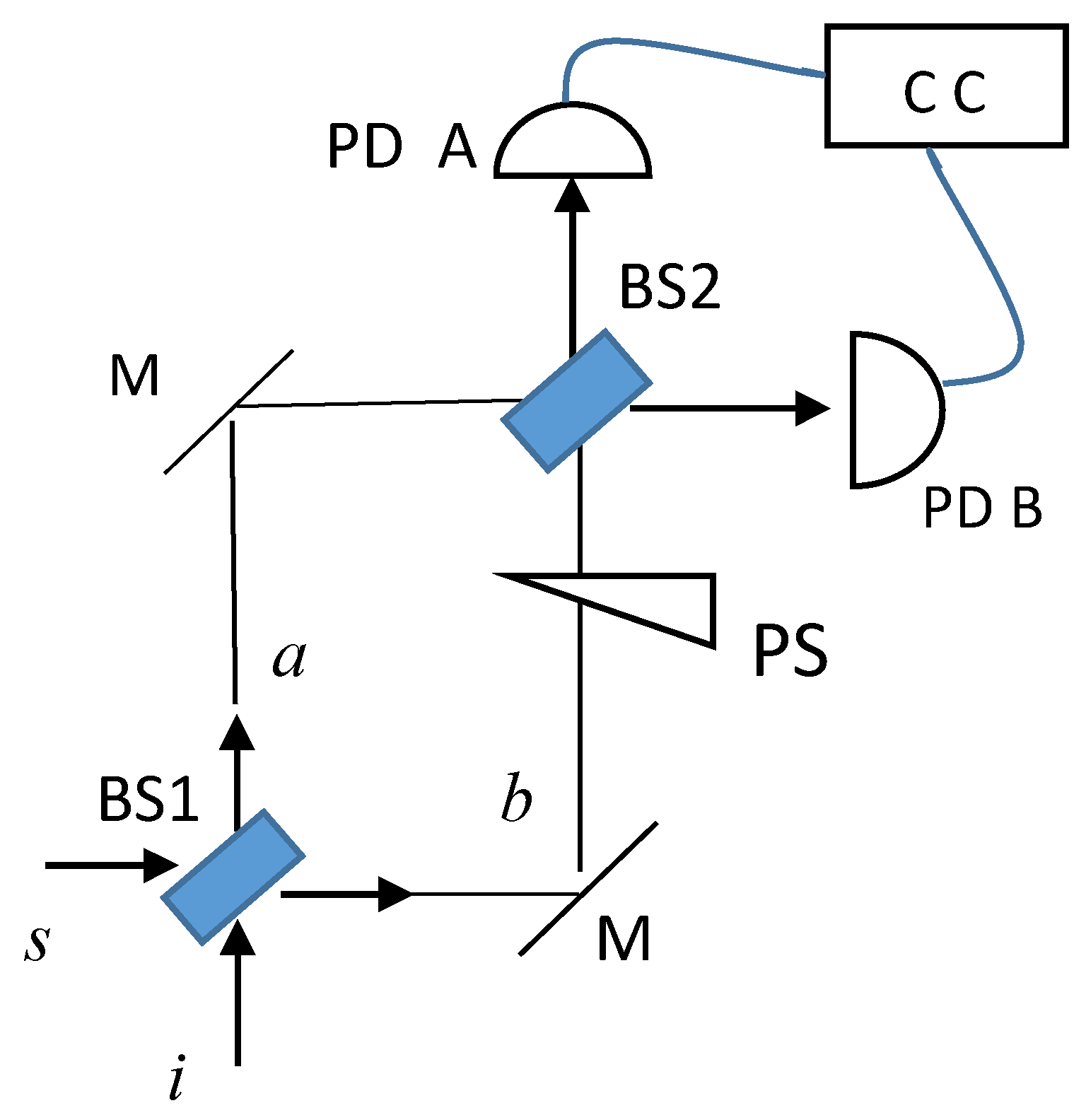
Example 4 - Next, we recall the parametric phase-pulling effect [15,23] leading to a phase correlation between the signal (s) and the idler (i) waves, i.e., , for any initial phases of weak waves such as spontaneous emission, with the coherent phase of the pump photons given by . As a result, at the either output A or B of the second cubic beam splitter of a 2 x 2 MZI as illustrated in Figure 2, one finds a constant phase relation
or the term [14] of the correlation function , with subscripts a and b denoting the two arms of the MZI, one of which may include a modulation or bias phase , and taking into account the phase shifts at the internal interfaces of the beam splitters. This phase relation will result in nonvanishing intensity correlations in the case of a 2 × 2 Mach-Zehnder interferometer. This equality of also applies to the two-source experiment outlined in Figure 3 of ref. [18] with subscripts a and b replaced by numbers 1 and 2,
respectively, as well as corresponding to the pump’s coherent phase modulation. In Figure 6 of ref. [18], the second source is driven by the idler beam from the first source so that , with being a bias phase of transition. Hence, one finds this phase equality so that, it is not “the relationship between interference and indistinguishability“ [18] that is responsible for the intensity interference but the phase pulling effect of which maximizes the parametric gain [15] (see Appendix A).
The random phases of the spontaneously emitted photons which are parametrically amplified in the crystal of their emission are missing from the conventional interpretation of the Hong-Ou-Mandel (HOM) dip [18,20]. By contrast, the random phases of a spontaneously emitted photon are directly associated with the dynamic and coherent number states composed of two consecutive number states which deliver c- numbers that behave in line with the Ehrenfest theorem of the time evolution of the expectation values [14,15].
Therefore, there is no need for entangled photons – apparently created by SPDC sources – which transcend time and space to have their probability amplitudes somehow interfere in order to explain the coincidence counting of photons by two separate photodetectors. The only requirement is that the two groups of photons are split between the two detectors – with an interface-induced phase – and are synchronized at the detection stage. Additional physical shortcomings of the Mandel approach based on entangled single photons are outlined in Appendix B emphasizing the confusion about the Dirac notation which requires a spatial integral to be evaluated, apparently ignored by the Glauber theory of detection [16].
5. Visibility of Unity Obtained with the Intrinsic Field of Independent Photons
For a minimum value of zero, any interference pattern will display a visibility of unity. It is claimed that in the quantum regime of one photon per radiation mode, the two-photon interference of the Hong-Ou-Mandel (HOM) dip is indicative of quantum features which cannot be obtained with a larger number of photons [18,19,20]. For example, the total anticorrelation of the HOM measurement for two indistinguishable photons will exhibit a unity visibility even though the local expectation values vanish. Similarly [20], “independent photons sent in different arms of a balanced interferometer always bunch and exit the interferometer from the same port. “
However, by controlling the three factors of the interference term such as in eqs. (16)-(18), the overall total visibility will reach unity for a ratio regardless of the number of photons. Intensity correlations with 100% visibility have been shown to be possible in Section 4 and brought about by the random phases of pulses [14,19] or the groups of photons created by the amplification of spontaneously emitted photons [14,15]. These physical elements can be found in the experimental results of ref. [21].
The overlap integral of the intrinsic fields of photons, i.e., is critical in the appearance of the anticorrelation dip because the photonic fields have the same distribution for any optical source [14]. This is in contrast to the concept of the time-independent superposition of one-photon states [20] leading to a one-photon state which is a superposition of many photons of frequencies even though only one photon is supposed to be in the system at any given time. This physical contradiction also applies to the two-photon state as described in ref. [20]. Nevertheless, Dirac’s notation is shorthand for a spatial integral over an operator , i.e., which is missing from ref. [20], in line with the convention of assuming a global state even though photon A cannot be detected at location B.
Equally, the conventional concept of ‘which way’ propagation argues [18] that “If the different possible photon paths from source to detector are indistinguishable, then we have to add the corresponding probability amplitudes before squaring to obtain the probability. This results in interference terms as in Eq. (3) (of ref. [18]). On the other hand, if there is some way, even in principle, of distinguishing between the possible photon paths, then the corresponding probabilities have to be added and there is no interference.” This would imply that an observer’s knowledge or lack thereof actually generates an effect. But how can the observer establish whether or not only a single photon is present without actually probing the link? This paradigm is negated by physically meaningful analyses in this article and experiments that prove that the HOM dip can occur with multiple photons [19,21].
The following fundamental question has never been addressed in the professional literature of quantum optics: How can a single photon propagate in a straight-line inside a dielectric medium given the presence of the quantum Rayleigh scattering of single photons? Articles dealing with the interpretations of one-photon and two-photon quantum interference such as refs. [18,19,20,21,22,24] ignore completely the existence of the quantum Rayleigh scattering of single photons [13] despite experimental demonstration of backward stimulated Rayleigh scattering in optical fibres [13,25] being analysed in refs. [14,15].
As explained previously [14,15], a spontaneously emitted photon in a parametric down-converting (SPDC) source is unavoidably amplified, which creates a group of identical photons that is capable of overcoming the quantum Rayleigh scattering of single photons as they cross a dielectric medium such as a beam splitter or a spectral filter. And the random phase of the spontaneous emission and related groups of photons play critical roles in obtaining a 100% visibility of the HOM dip by means of multi-photon states [14,15]. This is possible because a smooth transition from the quantum regime to the classical one is engendered by the dynamic and coherent number states [14,15] which deliver the number of photons and their complex amplitude carried by a wave front [14]. This type of interaction is capable of coupling one photon to another counter-propagating photon, when they reach the same electric dipole within the relevant interaction time [25]. The direction of coupling will depend on the relative phase between the two photons at the location of the electric dipole.
Additionally, the rather complex operation of a beam splitter in the quantum regime [15] involves the physical propagation and scattering of photons across the dielectric medium rather than the mathematical translation of a photon creation operator from input to output [24], i.e., which overlooks many physical interactions [14,15]. For example, in refs. [19,20,21,22], the spectral optical filter temporarily spreads the group of photons by repeated internal scatterings or partial reflections. Also, the phase-shifts and losses in the second beam splitter of an MZI need to be accounted for, as should the operation of a fibre-based beam splitter being different from that of a cubic beam splitter [14,15]. The operation of fibre-based couplers or beam splitters [14,15] depends on the input relative phase of the photons and this relative phase varies randomly, and so will the output.
While the detected output may vanish for a longer stretch of fibre illustrated in Figures 4 and 7 of [19] – used in a HOM experiment – because of the Rayleigh scattering, there may be photons reaching the second beam splitter as most of the ‘lost’ photons actually bounce back and forth inside the various components such as spectral filters, beam splitters, connecting fibers, etc. and will coalesce to form groups of identical photons through stimulated Rayleigh emission [13,25]. Figure 7 of ref. [19] actually displays three beam splitters.
The common assumption [20] is that the temporal signal g(t) of a monochromatic photon is the Fourier transform of the spectral distribution measured cumulatively at the output of the optical SPDC source – see eqs. (3-4) of [20], or page S281 of [18]. Yet, with only one photon reaching the detector at any given time, the Fourier transform cannot apply because it requires the simultaneous presence of all the spectral components. In fact, the mathematical formalism [18,20,24] confirms the ‘classical’ superposition of multiple photons as the wave packet functions are time- and space- independent. The temporal profile of a monochromatic photon was presented in eqs. (14), having been derived by combining the expectation values of the electrical and magnetic field operators for the dynamic and coherent number states [14]. The spontaneous emission was shown to include a random phase which leads to the vanishing of the field correlation. By contrast, the intensity correlation delivers an interference function as the phase fluctuations are shared by the multiplied photocurrents [14] as explained in Examples 3 and 4 of Section 4.
Consequently, the following statement of [20] is incorrect in saying that “We can see that the average zero correlation effect is caused by the φ dependent term, which is a first-order interference term. One can thus easily identify and isolate it and argue that quantum effects are associated with second-order correlation terms only. By keeping only these terms, it is clear that the HOM dip cannot be reproduced with classical fields”. This statement is incorrect because each and every single event will deliver an instantaneous value for the detection outcome, and the zero average will be calculated only at the end of the large ensemble of measurements, normalized to the number of events as opposed to being an average over a phase range. Thus, the instantaneous product of the photocurrents directed to a third location will be given by the first-order interference terms. This is, in fact, eq. (4) of ref. [20]. The distinction is made between pure quantum states of dynamic and coherent number states [14,15] which can accommodate instantaneously measured values and the mixed quantum states which can only provide information about average values only after the large ensemble of measurements has been completed.
Another article of interest for this subject is ref. [24], which states that “We define an interferometer as a device comprising only passive linear optical elements, principally beam splitters, mirrors and wave-plates, …“. However, the physical reality undermines this definition because of the quantum Rayleigh spontaneous and stimulated emissions occurring in such dielectric devices [13,14,25].
At low levels of photon numbers, the coherent state (CS) [16] is physically problematic as the annihilation operator leaves the state unchanged. While mathematically possible, a transition operator such as the photon annihilation operator, cannot have a physical eigenstate because such an operator changes the quantum state by its definition. The CS only delivers an expectation value at the output of an active medium by disregarding the photon-dipole interactions of other levels of the CS distribution which can change in the process. This is particularly so for parametric interactions which involve the local values of both the numbers of photons as well as the local phase of the photonic beam [14,15].
The existence of the quantum Rayleigh emissions in dielectric media [13] also contradicts a few deeply entrenched interpretations listed in ref. [24] such as: “Photons do not interact with each other, and any interference effects must be sought in the process by which each single photon passes from the source to the second screen. Quantum-mechanically, the interference occurs between the probability amplitudes for passage from source to screen via the two different paths corresponding to the two pinholes. The intensity on the second screen is proportional to the square modulus of the sum of the two probability amplitudes. The structure of the quantum-mechanical calculation is the same as that of the classical calculation, which is also based of the sum of two amplitudes, and the two calculations give the same intensity distribution.” These statements are unsubstantiated because they require that a photodetector should be able to anticipate or wait for the next photon to arrive through the other pathway. Physically meaningful interpretation for the correlations of outcomes have been provided in Section 4 above and, previously, in refs. [14,15].
Additional quotations from ref [24] read: “We consider two quantum interference phenomena that are not obtainable classically. These are photon antibunching and two-photon interference in the Hong-Ou-Mandel effect, both of which reveal themselves in the correlations between pairs of detectors”. However, as explained above in Section 4, the correlation consists of the electrical product of two local interference patterns. Once again, the quantum Rayleigh scattering of single photons prevents a single photon from propagating in a straight line. As derived in Example 3 above, the visibility is determined by an expression, eq. (18) containing the ratio of the numbers of photons for any level or total number of photons. Once again, the average or expectation values at the output are evaluated from the statistical distribution of an ensemble of measurements which is composed of instantaneous values. These individual values can be associated with pure dynamic and coherent states of photons [14] delivering the correct complex optical field and number of photons carried by a beam.
An SPDC source will unavoidably amplify the spontaneously emitted photons. Otherwise, the quantum Rayleigh scattering of single photons will prevent a straight-line propagation inside a dielectric medium. Consequently, quantum communication does not actually happen with 'entangled' photons but with groups of identical photons.
A recent and extensive review article [26] fails to explain the omission of the quantum Rayleigh spontaneous and stimulated emissions from the interpretation of experimental results. Equally,
in ref. [27], “a BS with transmissivity (with considered to be a classical control parameter) is inserted in path A of the MZI” also fails to explain the omission of the quantum Rayleigh spontaneous and stimulated emissions from the interpretation of experimental results, given the dielectric medium of the beam splitters.
6. Conclusions
It is the intrinsic fields of photons arising from the dynamic and coherent number states that bring about photonic detection and underpin interference fringes in both the quantum regime of several photons and the classical regime of many photons, rather than the mathematical concept of probability and its quantum amplitude. The probability is only determined at the output of the experimental setup after a large ensemble of measurements. By contrast, the intrinsic and instantaneous optical fields of photons are present at each and every detection of the ensemble.
The effect of quantum nonlocality is supposed to occur between the two entangled paired-photons for one setting at each detector, rather than between the quantum states of the two photodetectors identified by their respective angles of polarization. It should be emphasized that any quantum state, whether entangled or not, can give rise to the same correlation function which is obtained as a result of a well-known mathematical equality presented in the Introduction of this article.
No quantum mechanism has been identified that supports Glauber in his commentary on Dirac’s statement that ‘each photon then interferes only with itself’ [24]. The statement by Glauber that [28]: “The things that interfere in quantum mechanics are not particles. They are probability amplitudes for certain events. It is the fact that probability amplitudes add up like complex numbers that is responsible for all quantum mechanical interferences” is rather impossible because mathematical numbers averaged at the end of a long ensemble of measurements cannot be responsible for the outcome values of each and every individual measurement.
Physically meaningful interpretations of quantum correlations of photons have been provided consistent with published, but ignored, experimental results of independent photons rather than entangled ones. Despite an extensive review [26], the question of quantum Rayleigh scattering of single photons was not addressed. Equally, the suggestion that “since the behaviors of a photon are always concomitant with the configurations of experimental setup, one might envisage that the photon could adapt its behaviors in advance to the foregoing setting“ [27] takes the quantum community into the realm of speculation.
Data Availability Statement
The author declares that the data supporting the findings of this study are available within the paper which is based on the data published in the listed references.
Appendix A
The evolution of propagating beams of photons is analyzed based on the dynamic and coherent number states [14], i.e., whose evolution is given by the Ehrenfest theorem for the expectation values:
In a nonlinear crystal pumped, e.g., with a continuous wave (cw) and for frequency down-converted photons of angular frequencies satisfying or , the gain-providing medium generating the spontaneous emission, will also amplify the initially single photons of the signal and the idler, particularly so in the direction of wavevector matching conditions. As a result, the commonly assumed one single photon output does not, in reality, physically happen. At least several photons will be associated with each individual and discrete electronic “click”. The phase-dependent gain coefficient of such amplification, , and the rate of change of the relative phase are found from eqs. (A4) of ref. [15] to be:
Appendix B
The probability Pr over an ensemble of measurements, of joint or simultaneous detections in the time interval ] has the expression [18], based on Glauber’s theory of correlations [29]:
The probability of the HOM correlation vanishing for two groups of identical photons colliding inside a dielectric 2x2 beam splitter is easily explained by having the quantum Rayleigh stimulated emission induce coupling of photons from one group to the other [14,15], so that the resultant weaker group may not survive the propagation to the photodetector because of the quantum Rayleigh scattering of photons.
References
- E. Gent, “Quantum Computing’s Hard, Cold Reality Check: Hype is everywhere, skeptics say, and practical applications are still far away”; IEEE Spectrum, 22 Dec., (2023) https://spectrum.ieee.
- M. Brooks, “The race to find quantum computing’s soft spot”, Nature, Vol 617, 25 May 2023, pp. S1-S3.
- N. Brunner, D. Cavalcanti, S. Pironio, V. Scarani, and S. Wehner, ”Bell nonlocality,” Rev. Mod. Phys. 86, 419–478 (2014).
- M. Iannuzzi, R. Francini, R. Messi, and D. Moricciani,” Bell-type Polarization Experiment With Pairs Of Uncorrelated Optical Photons”, Phys. Lett. A, 384 (9), 126200, (2020).
- A. Ivashkin, D. Abdurashitov, Al. Baranov, F.Guber, S. Morozov, S. Musin, A. Strizhak and I.Tkachev, “Testing entanglement of annihilation photons”, Sci. Rep. 13:7559 (2023). [CrossRef]
- L. Santamaria Amato, D. Katia Pallotti, M. Siciliani de Cumis, D. Dequal, A. Andrisani, and S. Slussarenko, ”Testing the speed of “spooky action at a distance” in a table-top experiment,” Sci. Rep., (2023) 13:8201. [CrossRef]
- D. Salart, A. Baas, C. Branciard, N. Gisin, and H. Zbinden, “Testing the speed of ‘spooky action at a distance”, Nature (London) 454, 861-864 (2008).
- M. Giustina, et al., ‘‘Significant-Loophole-Free Test of Bell’s Theorem with Entangled Photons,’’ Phys. Rev. Lett. 115, 250401 (2015).
- L. K. Shalm et al., ‘‘Strong Loophole-Free Test of Local Realism,’’ Phys. Rev. Lett. 115, 250402 (2015).
- A. Aspect, “Closing the Door on Einstein and Bohr’s Quantum Debate,” Physics 8, 123, 2015.
- J. P. Gordon and H. Kogelnik, "PMD fundamentals: Polarization mode dispersion in optical fibers”, PNAS, vol. 97, no. 9, pp. 4541- 4550, 2000.
- A. Vatarescu, “Polarimetric Quantum-Strong Correlations with Independent Photons on the Poincaré Sphere,” Quantum Beam Sci., 2022, 6, 32.
- A. P. Vinogradov, V. Y. Shishkov, I. V. Doronin, E. S. Andrianov, A. A. Pukhov, and A. A. Lisyansky, “Quantum theory of Rayleigh scattering,” Opt. Express 29 (2), 2501-2520 (2021).
- A. Vatarescu, “Instantaneous Quantum Description of Photonic Wavefronts and Applications”, Quantum Beam Sci. 2022, 6, 29.
- A. Vatarescu, “The Quantum Regime Operation of Beam Splitters and Interference Filters”, Quantum Beam Sci. 2023, 7, 11.
- C. Garrison and R.Y. Chiao, Quantum Optics, Oxford University Press, 2008.
- R. Ursin et al., “Entanglement-based quantum communication over 144 km “, Nature Phys., vol. 3, pp. 481-486, 2007.
- L. Mandel, “Quantum effects in one-photon and two-photon interference,” 1 Rev. Mod. Phys., 71, S274-S282, 1999.
- S. Sadana, D. Ghosh, K. Joarder, A.N. Lakshmi, B.C. Sanders, U. Sinha, ”Near-100% two-photon-like coincidence-visibility dip with classical light and the role of complementarity,“ Phys. Rev. A 100, 013839 (2019). [CrossRef]
- N. Fabre, M. Amanti, F. Baboux, A. Keller, S. Ducci, and P. Milman, ”The Hong–Ou–Mandel experiment: from photon indistinguishability to continuous-variable quantum computing, “ Eur. Phys. J. D (2022) 76:196. [CrossRef]
- H. Kim, O. Kwon, and H.S. Moon, “Experimental interference of uncorrelated photons”, Sci. Rep., 9, 18375, 2019.
- J. G. Rarity, P. R. Tapster and R. Loudon, “Non-classical interference between independent sources”, J. Opt. B: Quantum and Semiclass. Opt., vol. 7, S171-S176, 2005.
- A. Vatarescu,,“Photonic Quantum Noise Reduction with Low-Pump Parametric Amplifiers for Photonic Integrated Circuits”, Photonics, 3, 61, 2016.
- S. M Barnett, “On single-photon and classical interference “, Phys. Scr. 97 (2022) 114004.
- T. Zhu, X. Bao, L. Chen, H. Liang, and Y. Dong, “Experimental study on stimulated Rayleigh scattering in optical fibers”, Opt. Express, 18, 22958-64, (2010).
- Z. Zhang, C. You, O. S. Magaña-Loaiza, R. Fickler, R. de J. León-Montiel, J. P. Torres, T. S. Humble, S. Liu, Y. Xia, and Q. Zhuang, “Entanglement-based quantum information technology: a tutorial “, Adv. Opt. Photon. 16(1), 60-162 (2024).
- Q.F. Xue, X. C. Zhuang, N. Ba An, D. Y. Duan, R. D. Ma, W.W. Pan, Q. Q. Wang, Y. J. Xia, and Z.X. Man “Single- and two-photon wave-particle superpositions: Theory and experiment”, Phys. Rev. A, 108, 022223 (2023).
- R. J. Glauber, “Dirac’s famous dictum on interference: one photon or two?” Am. J. Phys. 63 12, 1995.
- R. J. Glauber, ”Coherent and incoherent states of the radiation field”, Phys. Rev. 131 2766–88, 1963.
- T. Legero, T. Wilk, A. Kuhn, and G. Rempe, “Time-resolved two-photon quantum interference,” Appl. Phys. B 77, 797–802 (2003).
Figure 1.
The HOM setup. BS beam splitter; C C coincidence counting of photons; PD photodetector; IF interferometric filter. For the quantum regime operation of a beam splitter see ref. [15].
Figure 1.
The HOM setup. BS beam splitter; C C coincidence counting of photons; PD photodetector; IF interferometric filter. For the quantum regime operation of a beam splitter see ref. [15].
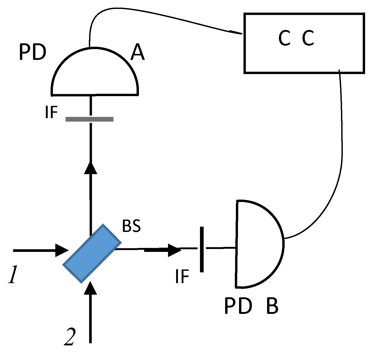
Figure 2.
Correlation setup for two intensities generated at two separate photodetectors with a Mach-Zehnder configuration. BS beam splitter; M mirror; PS phase shifter; PD photodetector; CC coincidence counting of photons. For the quantum regime operation of a beam splitter see ref. [15].
Figure 2.
Correlation setup for two intensities generated at two separate photodetectors with a Mach-Zehnder configuration. BS beam splitter; M mirror; PS phase shifter; PD photodetector; CC coincidence counting of photons. For the quantum regime operation of a beam splitter see ref. [15].
Disclaimer/Publisher’s Note: The statements, opinions and data contained in all publications are solely those of the individual author(s) and contributor(s) and not of MDPI and/or the editor(s). MDPI and/or the editor(s) disclaim responsibility for any injury to people or property resulting from any ideas, methods, instructions or products referred to in the content. |
© 2025 by the authors. Licensee MDPI, Basel, Switzerland. This article is an open access article distributed under the terms and conditions of the Creative Commons Attribution (CC BY) license (http://creativecommons.org/licenses/by/4.0/).
Copyright: This open access article is published under a Creative Commons CC BY 4.0 license, which permit the free download, distribution, and reuse, provided that the author and preprint are cited in any reuse.


