
Submitted:
25 April 2025
Posted:
25 April 2025
You are already at the latest version
Abstract
A miniaturized hyperspectral camera, developed by integrating a linear variable band-pass filter (LVBPF) with an image sensor, was installed on the TIRSAT 3U CubeSat, launched on February 17, 2024, by Japan’s H3 launch vehicle. The satellite and its onboard hyperspectral camera conducted on-orbit experiments and successfully acquired hyperspectral data from multiple locations. The required attitude control for the hyperspectral mission was also achieved. CubeSat-based hyperspectral missions often face challenges in image alignment due to factors such as parallax, distortion, and limited attitude stability. This study presents solutions to these issues, supported by actual observational hyperspectral data. To verify the consistency of the hyperspectral data acquired by TIRSAT and processed using the proposed method, a validation analysis was conducted.
Keywords:
hyperspectral camera
; CubeSat mission
; hyperspectral imaging
; geometric transformation
; on-orbit performance
1. Introduction
Hyperspectral cameras are valuable tools for Earth observation, supporting a wide range of applications such as agricultural, forestry, and ocean remote sensing. These cameras capture both images and spectral data simultaneously, enabling the detection and classification of target conditions [1,2,3,4]. Although several operational systems and development plans exist for hyperspectral cameras on large satellites and the International Space Station [5,6,7,8,9], these remain limited in number, and their effectiveness has not been fully demonstrated. Ideal attributes for hyperspectral remote sensing include full Earth coverage and high observation frequency. This is particularly critical in agricultural monitoring, where frequent and regular observations are essential for effective crop management. However, when relying on a single satellite, the observation frequency remains low (approximately once every two weeks). A promising solution is the deployment of a constellation of CubeSats equipped with hyperspectral cameras.
Traditionally, spaceborne hyperspectral cameras have required large telescopes to gather sufficient light for spectroscopic observations. Recent advances in image sensor technology have significantly improved sensitivity, making hyperspectral imaging feasible even with smaller telescopes. Consequently, new initiatives are underway to deploy microsatellites and CubeSats with hyperspectral capabilities. In recent years, numerous start-up companies have entered the Earth observation sector, focusing on the mass production of small and microsatellites and offering services through satellite constellations. A satellite constellation refers to a system in which multiple microsatellites are interconnected and operated in a coordinated manner. Start-up companies are increasingly constructing such constellations to create a global Earth observation network [10,11,12,13,14]. Integrating hyperspectral cameras into CubeSats and microsatellites can significantly enhance the temporal resolution of Earth observation data collection.
Examples of compact hyperspectral cameras include HYPSO-1, developed by the Norwegian University of Science and Technology [15], and HyperScout-1, developed by Cosine Remote Sensing B.V. [16]. Dragonette, developed by Canada’s Wyvern, has a wavelength resolution of 20 nm, resulting in coarser spectral data than some alternatives. However, it achieves a ground sampling distance of 5.3 m, allowing for higher spatial resolution imaging [17]. Kuva Space, a Finnish hyperspectral satellite start-up, aims to provide global images two to three times daily using a constellation of 100 6U CubeSats called Hyperfield, which will cover the spectral range from visible near-infrared to short-wavelength infrared [18]. Planet’s Tanager satellite is equipped with a hyperspectral sensor that spans wavelengths from 400 nm to 2500 nm. While many small satellites are limited to visible and near-infrared observations, Tanager’s ability to extend into the short-wavelength infrared range (up to 2500 nm) is a key advantage [19]. In this range, methane absorbs between 2150 and 2450 nm, and CO₂ absorbs between 1980 and 2100 nm. This capability enables the distinct detection of CO₂ and methane, contributing to efforts toward carbon neutrality.
In this context, the University of Fukui and SEIREN CO., LTD. developed and installed a hyperspectral camera on a CubeSat named TIRSAT and conducted an in-orbit demonstration. TIRSAT is a 3U CubeSat developed primarily by SEIREN CO., LTD., managed by Japan Space Systems as a commissioned project for Japan’s Ministry of Economy, Trade and Industry (METI). TIRSAT’s primary payload is a bolometer-type camera intended for thermal infrared measurements of Earth’s surface temperature, including heat sources such as factories to estimate operational status. The hyperspectral camera developed by the University of Fukui was installed as an additional payload for in-orbit demonstration. TIRSAT was successfully launched into a sun-synchronous sub-recurrent orbit at an altitude of approximately 680 km on February 17, 2024, by Japan’s H3 launch vehicle. After orbit insertion, the satellite’s basic functions were verified, and mission operations began. The hyperspectral camera on TIRSAT incorporates a linear variable band-pass filter (LVBPF), enabling significant miniaturization suitable for CubeSat integration [20]. This advancement allows for convenient spectral measurement of ground features and expands the potential of hyperspectral imaging applications. The camera can be easily integrated into CubeSats carrying multiple instruments and is particularly effective for hyperspectral CubeSat constellations.
This paper presents detailed performance specifications of the hyperspectral camera, along with the satellite’s specifications and attitude control results related to TIRSAT observations. It also provides an analysis of the observational data and the in-orbit data processing methods. In particular, LVBPF-based hyperspectral data processing requires precise image alignment, which is critical for data accuracy. This paper proposes a geometric transformation-based alignment method to correct image distortion and discusses the validity of the acquired hyperspectral data.
2. Development of a Linear Variable Band-Pass Filter-Based Hyperspectral Camera
2.1. Observation Method of LVBPF-Based Hyperspectral Camera
Conventional hyperspectral cameras typically consist of a telescope and a slit-based spectrometer, which includes a collimator, a dispersion element (usually a prism or grating), and an objective lens. Due to the numerous optical components required, such cameras are difficult to miniaturize, particularly for space applications where suitable optical materials are limited. Recently, a miniaturization method employing a linear variable band-pass filter (LVBPF)—a band-pass filter whose wavelength transmittance changes linearly with position—has been proposed [21,22,23,24]. This approach enables the acquisition of both spatial and spectral information using a single, compact filter.
The configuration and observation mechanism of the LVBPF-based hyperspectral camera is shown in Figure 1. While traditional grating-based hyperspectral cameras offer high spectral resolution, they reduce the amount of light reaching the image sensor due to the dispersion of incident light into multiple orders. In contrast, the sensitivity of an LVBPF-based camera primarily depends on the transmittance of the filter, resulting in higher sensitivity. However, as with conventional types, LVBPF-based hyperspectral cameras also require push-broom scanning. The filter’s wavelength transmittance varies in the along-track direction, necessitating image acquisition at different positions to capture data at the same wavelength. These spectral images are then assembled into three-dimensional hyperspectral data.
2.2. Specification
In this study, a miniaturized hyperspectral camera utilizing an LVBPF was developed and installed as an additional payload on the 3U-CubeSat TIRSAT. Figure 2 shows the development of the LVBPF-based camera. The unit, including the lens, filter, and image sensor, was approximately 3 cm long and weighed only 35 g. This compact design allows integration not only into 3U-CubeSats but also into 1U-CubeSats.
Table 1 lists the camera specifications. Since the hyperspectral camera was designed as an auxiliary instrument aboard a multi-mission CubeSat, a small lens with coarse resolution was selected to ensure a wide ground coverage of up to 450 km. Table 2 presents the LVBPF specifications. The filter, which was tailored to match the size of the image sensor, enables coverage of visible to near-infrared wavelengths. As shown in Figure 2, the filter was not deposited directly onto the sensor but mechanically fixed. To achieve minimal spacing, the image sensor’s cover glass was removed, and the filter was positioned as close as possible to the sensor.
This design offers flexibility, allowing easy modification of spectral resolution and wavelength range by changing the filter, sensor, or telescope lens. The image sensor used was the UI-1242LE-NIR from IDS Imaging Development Systems GmbH. It features a global shutter, making it suitable for space applications. The system utilizes a USB 2.0 interface, and imaging control was executed using a Raspberry Pi Compute Module 3. Additionally, onboard image processing using Python and OpenCV was supported, resulting in a highly flexible camera system based on consumer-grade technology.
2.3. Pre-Flight Test on Ground
2.3.1. Imaging Performance
The imaging performance of the hyperspectral camera flight model was evaluated in ground tests. Point spread functions (PSFs) were measured using a collimator with a pinhole chart illuminated by green light. Environmental tests included random vibration, thermal cycling, and thermal vacuum testing. The thermal tests simulated expected space conditions, ranging from −10 °C to +50 °C. The random vibration test was conducted with the camera mounted on the TIRSAT flight model, following the launch vehicle specifications.
Figure 3 shows the PSFs measured before and after environmental testing. Prior to testing, the PSFs exhibited a standard deviation (σ) of 1.4 pixels, indicating good imaging quality. After the tests, the vertical axis PSF increased slightly to 1.6 pixels, while the horizontal axis remained at 1.4 pixels. The overall change in PSF was 0.2 pixels. Despite this minor deviation, the camera maintained sufficient imaging performance, demonstrating its robustness under launch and space conditions.
2.3.2. Spectral Performance Measurement and Calibration
Spectral performance was evaluated using an integrating sphere equipped with a 10 nm full width at half maximum (FWHM) band-pass filter and illuminated by a halogen lamp. The band-pass filter allowed specific wavelength ranges to pass, enabling assessment of the camera’s spectral resolving ability. A halogen lamp provided stable, broad-spectrum illumination for consistent and accurate spectral measurements.
Spectral images were acquired by the hyperspectral camera flight model at discrete wavelengths corresponding to band-pass filters centered at 400 nm, 450 nm, 500 nm, 550 nm, 600 nm, 650 nm, and 700 nm, as shown in Figure 4. These images were analyzed to calibrate the spectral data and evaluate the resolution at each wavelength. The raw images exhibited noticeable distortion, characterized by a pronounced smile effect. This distortion, commonly caused by optical components such as lenses, was uncorrected in the acquired images. Additionally, positional variation in the wavelength transmission of the LVBPF contributed to the overall distortion.
Figure 5 quantitatively illustrates the smile distortion. The center of gravity was calculated for each image column, and the center positions were plotted against the row number. The resulting data revealed a shift of approximately 20–30 pixels from the center to the image edge. Using a calibration coefficient of 0.336 nm/pixel, calculated at the central row (512 pixels), this displacement corresponds to a wavelength shift of approximately 6.72–10.08 nm. Although relatively small, this shift significantly affects spectral accuracy and cannot be ignored.
To address this, a wavelength calibration formula was calculated for each row based on the spectral data in Figure 4. The results were used to generate a calibrated wavelength map, presented in Figure 6. This map allows for accurate wavelength assignment across the entire image and compensates for distortion-related errors. The implications of this calibration will be further discussed in the section on observed image analysis.
Figure 7 shows the spectral resolution at the image center (row 512) for each band. The resolution values were as follows: 49.5 pixels (16.6 nm) at 400 nm; 56.5 pixels (18.9 nm) at 450 nm; 61.1 pixels (20.6 nm) at 500 nm; 68.3 pixels (23.0 nm) at 550 nm; 87.1 pixels (29.3 nm) at 600 nm; 110.7 pixels (37.2 nm) at 650 nm; and 113.0 pixels (38.0 nm) at 700 nm. Spectral resolution was interpreted as the width of the light beam passing through the filter, calculated as the product of the reciprocal F-number, dispersion, and distance between the filter and the focal plane. With an F-number of F/2.5, a filter-to-focal-plane distance of 0.67 mm, and a dispersion of 67.7 nm/mm, the theoretical spectral resolution was approximately 18.1 nm.
Measured and theoretical values showed good agreement at shorter wavelengths; however, resolution became coarser at longer wavelengths. This trend likely resulted from the wavelength-dependent half-bandwidth of the LVBPF, which is broader on the long-wavelength side, increasing the allowable incident angle and reducing resolution. These factors increase spectral cross-talk among adjacent pixels, degrading spectral purity and reducing the effective number of bands.
To meet the mission’s requirements, the camera was equipped with a fast F/2.5 lens to capture high-quality Earth images. However, this lens increased the beam width through the filter, resulting in coarser resolution. The dependence of spectral resolution on lens F-number was confirmed and should be considered in future optimization of LVBPF-based hyperspectral camera design.
3. Description of Satellite Bus for TIRSAT
3.1. Introduction of TIRSAT
This section outlines the specifications of the TIRSAT satellite. An external view of the satellite flight model is shown in Figure 8. The satellite measured 117 mm × 117 mm × 381 mm before the deployment of its solar array panels and had a mass of 4.97 kg. It was equipped with a 1U-sized (approximately 100 mm × 100 mm × 100 mm) bolometer-type camera that operated in the thermal infrared wavelength range as its primary mission payload. Accordingly, the satellite bus occupied approximately 2U of volume. The main specifications of the TIRSAT satellite bus are summarized in Table 3, and its mechanical configuration is illustrated in Figure 9.
The satellite bus, named SRN-3U, was developed by SEIREN CO., LTD. in collaboration with the University of Fukui and the University of Tokyo. It was based on the flight heritage of the TRICOM-2 satellite bus [25,26], with enhancements including high-speed communication capability, high-precision attitude control, and deployable solar panels. The satellite was designed to be compatible with the ISI Space Quad Pack Type III CubeSat deployer, which matches the release mechanism dimensions of the H3 launch vehicle.
The ground station, equipped with S-band and X-band antennas, is located at ArkEdge Space in Japan. Satellite operations, including pass scheduling, mission planning, and data analysis, are conducted at SEIREN’s satellite operation center in Fukui, Japan. Hyperspectral data acquired by TIRSAT is analyzed at the University of Fukui.
TIRSAT was equipped with an X-band transmitter capable of downlink speeds up to 10 Mbps. It used two types of X-band antennas: a broad-directional low-gain antenna (LGA) and a highly directional medium-gain antenna (MGA). For telemetry and command, an S-band transponder was employed, with antennas mounted on the +Y and −Y panels. These antennas were connected via an RF combiner and splitter, enabling communication in nearly all directions by covering half the space in the +Y or −Y direction.
The satellite also featured four deployable solar panels that could generate up to 20 W of effective power. In addition, body-mounted solar cells were installed on four sides of the satellite. This redundant configuration supported stable power generation during the initial operational phase and ensured the power budget was maintained even if sun-pointing control was lost. The satellite's battery consisted of lithium-ion cells arranged in a 2-series, 2-parallel configuration.
The attitude determination and control subsystem (ADCS) was based on a compact 1U-sized integrated module [27], which was customized for this mission by excluding a star tracker. The onboard computer (OBC) was derived from the TRICOM-2 project and featured a fault-tolerant design that included automatic rebooting approximately every four hours via a reset counter, regardless of operational mode. This served as a countermeasure against single-event faults. Status data was recorded in high-speed, non-volatile memory and retrieved immediately after reboot to ensure continuous operation.
Both the ADCS and OBC employed a command-centric architecture (C2A) for software implementation [28], providing high flexibility and ease of in-orbit reconfiguration. This architecture defined all satellite actions through commands, enabling functional changes without memory rewriting and allowing software updates to be implemented efficiently in orbit.
3.2. Attitude Determination and Control Subsystem of TIRSAT
The block diagram of ADCS is presented in Figure 10, and its specifications are summarized in Table 4. TIRSAT employed a three-axis attitude control system composed of two microelectromechanical systems (MEMS) gyroscopes, three sun sensors, two geomagnetic sensors, three-axis reaction wheels, and three-axis magnetic torquers, all integrated into a compact ADCS module. Redundant units were included for both the gyroscopes and geomagnetic sensors, with one unit offering fine accuracy and the other coarse accuracy.
Although the ADCS module included a Global Navigation Satellite System Receiver (GNSSR), onboard position determination was primarily performed using the Simplified General Perturbations Satellite Orbit Model 4 (SGP4) and two-line elements (TLEs) uploaded from the ground station. During orbital operations, SGP4 with TLEs was predominantly used for position estimation.
The ADCS software supported multiple control modes, including detumbling using only magnetic torquers, three-axis nadir pointing, and three-axis sun pointing. Each pointing mode was achieved using a combination of three-axis reaction wheels and magnetic torquers, or with magnetic torquers alone. Thus, even in the event of a reaction wheel failure, attitude control could continue with reduced accuracy. Additionally, an offset angle could be applied to each of the three rotational axes—roll, pitch, and yaw—in any pointing mode. As the ADCS was not equipped with a star tracker, attitude determination relied mainly on sun sensors, which offered an accuracy of approximately 0.5°.
A software-in-the-loop simulation (SILS) was conducted to validate the nadir-pointing control mode. The initial angular velocity for all axes was set to 0.1°/s, and the simulation commenced under daylight conditions. The satellite was assumed to be in a Sun-synchronous orbit at an altitude of 580 km. Initial attitude conditions were defined such that in Case A, the −X surface was oriented toward the Sun, while in Cases B to D, offset angles were applied to each axis. As shown in Figure 11, the simulation results indicated that the attitude convergence time was within 400 seconds and the pointing error was maintained within 2°. Furthermore, after 3000 seconds, the attitude remained stable with a pointing error of less than 1°.
The target values for attitude control in the hyperspectral imaging mission are presented in Table 5. The target pointing control angle was set to 7.3°, corresponding to a positional difference of 200 pixels between the target location and the captured image. Because the hyperspectral camera utilized a linear variable band-pass filter (LVBPF), spectral direction pixels had to align with the along-track direction. As a result, high precision was required for yaw-axis attitude control and roll-axis attitude stability. A conceptual diagram illustrating these requirements is shown in Figure 12.
The required yaw-axis attitude accuracy was derived using Equation (1), where α denotes the acceptable overlap ratio between the first and last images, and IFOV (instantaneous field of view) represents the angle per pixel, which was 0.038° for the hyperspectral camera. Assuming an allowable overlap ratio of 70%, the required yaw-axis pointing accuracy was calculated to be 5.8°. Moreover, the roll-axis angle during imaging needed to be maintained within 5.8° of its initial value.
The required image capture duration was calculated using Equation (2). At an orbital altitude of 680 km, TIRSAT’s orbital velocity was approximately 7.5 km/s, and its ground sampling distance (GSD) was 450 m/pixel, as shown in Table 1. Given an along-track pixel count of 1024, the required image capture time was estimated to be approximately 120 seconds. During this period, the roll-axis angle had to remain within 5.8°, yielding a required attitude stability of 0.048°/s. Based on the SILS results, the ADCS of TIRSAT demonstrated sufficient capability to meet these pointing and stability requirements.
3.3. Mission Data Handling and Communication Subsystem
The control of the mission payload, including the hyperspectral camera, was managed by the mission data handling unit (MDH), which was developed using a field-programmable gate array (FPGA). Mission data transmission to the ground station was carried out using the X-band transmitter. The block diagram of the mission processing and communication subsystem is shown in Figure 13. As previously mentioned, the hyperspectral camera was controlled by a Raspberry Pi. Captured images were transferred to the MDH via Serial Peripheral Interface (SPI) communication. The MDH stored the received raw images in the embedded multimedia card (eMMC) memory, which served as the data storage. The eMMC memory had a total capacity of 8GB, with 1GB allocated for the hyperspectral camera. The data read from the eMMC memory was transmitted to the ground station through the X-band transmitter, using a data format compliant with the Consultative Committee for Space Data Systems (CCSDS) standard.
To perform map projection, satellite attitude and position data corresponding to the image timestamp were required. These ancillary data were transmitted from the ADCS module and transferred to the hyperspectral camera via the onboard computer (OBC) and MDH. The ancillary data were appended to the header of the raw image and also stored in the eMMC memory. The MDH and eMMC memory utilized commercial off-the-shelf (COTS) components, which were newly developed. It was confirmed that these components had a radiation tolerance exceeding 20 krad. Proton irradiation experiments also evaluated their single-event resilience, and the results confirmed that these components were sufficiently capable of functioning in orbit.
The X-band transmitter supported downlink communication speeds of 5 Mbps or 10 Mbps using Offset Quadrature Phase Shift Keying (OQPSK) modulation. The output power of the transmitter could be set to 1 W or 2 W. TIRSAT was equipped with a single patch array antenna as the Low Gain Antenna (LGA) and a 2×2 patch array antenna as the Medium Gain Antenna (MGA). These antennas could be switched using an RF switch. The maximum gain of the LGA was 4 dBi, while the MGA had a maximum gain of 10 dBi. The LGA was mounted on the +Y surface, and the MGA was mounted on the −Y surface. The half-power beamwidth was ±35° for the LGA and ±20° for the MGA. While attitude control was required during X-band communication, coarse attitude control sufficed when using the LGA.
4. Data Construction Method for LVBPF-Based Hyperspectral Data
The images acquired using an LVBPF capture different transmission wavelengths in the along-track direction. Therefore, a single image represents a mixture of spatial and spectral information. Spectral images are captured at various positions using push-broom observations to capture the same wavelength, with the overlapping parts of each image synthesized to generate a spectral image, forming hyperspectral data. In general, push-broom imaging sequentially synthesizes images at regular intervals. However, factors such as lens distortion, parallax at the capture position, and attitude instability can affect image alignment. As a result, when overlapping regions are synthesized using only temporal capture information, the resulting hyperspectral data exhibit distortions, and the individual spectral images do not align properly. To address this, we estimated overlap coordinates using image feature point matching and homography transformation, synthesizing the images to generate corrected hyperspectral data.
The data construction method is illustrated in Figure 14. This process is divided into two stages. The first step involves feature point matching to automatically detect the overlapping regions of each image. Displacement between the images is then estimated, and alignment is achieved using affine transformation. The images used in this step are raw data captured by the LVBPF-based hyperspectral camera, referred to as RAW images. Each RAW image is accompanied by a wavelength map that indicates the transmission wavelength for each pixel, as shown in Figure 6. These RAW images contain distortions due to lens and parallax effects and represent unprocessed data. Feature point matching is performed between the first image (In) and the following image (In+1). To facilitate feature point matching, the RAW images undergo image enhancement processes such as contrast enhancement and sharpening. Gamma correction was applied for contrast enhancement, and unsharp masking was used for sharpening. Accelerated Keypoint and Descriptor Extraction (AKAZE) was employed for feature point detection.
After applying these enhancements, the top three feature point pairs identified were selected, and affine transformation was performed. The wavelength map was transformed using the same matrix applied to the images. This process was repeated for each image captured by the hyperspectral camera, yielding affine-transformed RAW images and corresponding wavelength maps, which were stored in a three-dimensional structure to form the hyperspectral data.
At this stage, the RAW image and wavelength map were affine-transformed, meaning only operations such as translation or rotation were applied. While this step resulted in roughly aligned hyperspectral data, distortions due to parallax and other factors were not removed, and the images did not align perfectly. The next step involved performing a homography transformation based on feature point matching between the generated hyperspectral data to correct position and distortion simultaneously. The result was distortion-free and properly aligned hyperspectral data.
The spectral images for each band were read from the hyperspectral data, and the positions of feature points were extracted. Feature point detection and extraction were performed using the same method as in the first step. The complete set of extracted feature point pairs was then used with Random Sample Consensus (RANSAC) to compute the homography transformation matrix. RANSAC is an iterative algorithm used to estimate a model from data containing outliers. All spectral images, except for the reference image, were transformed using this matrix and stored in the final hyperspectral data.
5. On-Orbit Result
5.1. Observation Result and Validation of Data Construction Method
TIRSAT successfully pointed to the nadir, scanned, and acquired ground surface images using the LVBPF-based hyperspectral camera. The first hyperspectral data was acquired on March 29, 2024, with data acquisition continuing thereafter, incorporating parameter adjustments for precise attitude control. Several hyperspectral datasets acquired by TIRSAT are presented. These datasets were constructed using the method outlined in Figure 14. Figure 15 shows a composite color image created using the red, green, and blue spectral bands, acquired near Baja California, Mexico. The image reveals spectral data for various regions: the ocean (e.g., location A), urban areas (e.g., location B), and mountainous areas (e.g., locations C and D). Next, Figure 16 displays data captured over Romania and Bulgaria, including spectral data for vegetation areas (e.g., locations A, B, and D) and bare land (e.g., location C). Figure 17 shows a false-color image generated using data collected near Nevada, USA, including spectral information from vegetated areas (e.g., locations A, B, C, and D).
To demonstrate the effectiveness of the proposed hyperspectral data construction method, several methods are compared: (1) the sequentially synthesized method at regular time intervals, (2) affine transformation, (3) homography transformation, and (4) the proposed method, which combines both affine and homography transformations. Table 6 provides the parameters for each method. Figure 18 illustrates examples of positional shifts caused by the data construction methods. The base data, taken near Kazakhstan, show comparisons of overlap for the red, green, and blue bands at three locations, using the four methods. The results reveal that, at the central location (b), all methods provide relatively accurate alignment. However, significant positional shifts are observed at the other locations (a and c), where the bands do not overlap correctly, except for the proposed method.
If orbital velocity were the only factor, alignment could be achieved using the sequentially synthesized method or affine transformation, but distortion would still occur. Specifically, the hyperspectral camera installed on TIRSAT is a wide-angle camera, and due to the Earth’s curvature and parallax, the height difference between the center and edges of the image exceeds 40 km. As a result, affine transformation alone cannot remove distortion. Homography transformation can correct geometric distortions in the image, but it cannot fully account for distortions caused by Earth’s curvature and parallax, nor can it completely convert the image into a flat representation. Therefore, as proposed in this research, it is best to first generate hyperspectral data with coarse alignment using affine transformation to account for parallel movement, followed by homography transformation to correct distortions such as parallax. These results confirm the effectiveness of the proposed hyperspectral data construction method.
5.3. On-Orbit Analysis Results of the Satellite Bus Performances
5.3.1. Evaluation of Attitude Precision and Stablity
The attitude control accuracy and stability of TIRSAT were analyzed based on imaging data captured by the hyperspectral camera and attitude determination data from the ADCS. The attitude control accuracy was calculated based on the geometric correction accuracy of the images. Geometric correction was first applied to the raw images using attitude determination data, which included quaternions and satellite position, followed by map projection. Landsat-9 OLI-2 served as the reference data for verifying the accuracy of the geometric correction. Mexico, selected for its clear coastal features, was chosen as the sample location. Figure 19 shows the map projection results for the raw image and the geo-referenced image captured by Landsat-9. The verification location was the coastal area of Mexico, known for its clear features. Figure 19 illustrates the map projection results of the raw image captured by the TIRSAT hyperspectral camera, compared with the geo-referenced image from Landsat-9. Six ground control points (GCPs) were manually selected, and the distances between pairs were calculated and used to determine the geometric correction errors. The results are summarized in Table 7. The average geometric correction error was found to be 54.6 km, which, when converted to pointing error, corresponds to approximately 4.6°. This pointing error includes both attitude control errors and errors from the camera's shutter timing and alignment. However, the results satisfied the required values presented in Table 5.
Attitude stability was evaluated using the time history of angular velocity from the gyroscope onboard the ADCS. Figure 20 shows the time histories of angular velocity for all three axes, with an expanded graph for the roll axis. The time axis is referenced from the start of imaging, set as the zero-second point. TIRSAT's hyperspectral camera specifies a stability requirement for the roll axis of approximately 0.048°/s. The results show that, from the start to the end of imaging over a period of approximately 120 seconds, the angular velocity remained below 0.04°/s, thus meeting the stability requirement. Based on these analysis results, it can be concluded that the attitude control system of TIRSAT has sufficient performance to perform imaging with the hyperspectral camera.
5.3.2. Thermal Analysis
This section presents the thermal environment of the hyperspectral camera, based on thermal analysis results. While resistance temperature detectors (RTDs) are installed on each panel and certain components, the hyperspectral camera onboard TIRSAT does not have its own dedicated RTD. However, thermal simulations confirmed that the aluminum panel located adjacent to the camera exhibits similar temperature characteristics, allowing it to serve as a proxy for monitoring the camera’s temperature. Thus, the temperature of the aluminum panel near the camera was monitored and evaluated in orbit as a proxy for the camera’s temperature.
Figure 21 shows a comparison between the thermal simulation results and on-orbit measured data when the satellite was at an altitude of 680 km and in a tumbling state. The satellite can maintain its power budget even without sun-pointing, as its attitude control mode allows it to remain in a tumbling state with no attitude control during normal operations. The graph includes the simulated temperature of the hyperspectral camera and the panel near the camera, along with the on-orbit measured temperature of the panel. The simulation results generally match the on-orbit measurements, with the simulated camera temperature ranging between +6°C and -5°C. However, around the 65,000-second mark, deviations were observed, with temperatures approximately +10°C higher and -5°C lower than the simulated temperature at certain points. Further investigation is required to determine the cause of these discrepancies. Despite this, the hyperspectral camera was successfully operated in ground tests within the temperature range of -10°C to 50°C, indicating sufficient thermal margin for its operation.
5.3.3. Power Control Subsystem
TIRSAT is equipped with four deployable solar panels, which were successfully deployed in orbit, confirming a maximum effective power output of 16 W. Figure 22 illustrates the power generation status after the deployment of the solar array panels. Each deployable solar panel generated 4 W, resulting in a total power output of 16 W from all four panels. Power generation from the body-mounted solar array panels, previously obscured by the deployable panels, was also confirmed.
Power consumption increases during hyperspectral camera observations and X-band data transmission. To evaluate the power budget, Figure 23 and Figure 24 show the battery voltage profiles during observation and transmission periods, respectively. The onboard battery has a maximum voltage of approximately 8.0 V and maintains a nearly fully charged state under steady sunlight conditions. Figure 23 shows the battery voltage and power consumption of the hyperspectral camera during observations. The camera consumes approximately 2 W, and the battery voltage decreases by only about 0.5 V. This minor drop does not pose any issues, as the voltage returns to its original level once the observation is completed. Figure 24 shows the battery voltage and power consumption of the X-band transmitter during data transmission. The transmitter consumes over 10 W, and the battery voltage drops by approximately 0.9 V during transmission, indicating a significant decrease. The battery’s state of charge (SOC) is estimated to decrease from approximately 80% to 72% during this period. Nevertheless, data transmission is sustained for approximately 7 minutes. Given that the satellite's visible operation window is around 10 minutes, a 7-minute transmission duration is considered reasonable. These results confirm that TIRSAT's power budget is sufficient to support both hyperspectral observations and X-band data transmission.
5.4. Comparison of Hyperspectral Data Across Two Time Periods
A comparison of hyperspectral data from two time periods was conducted using datasets from the coastal area of Mexico, as shown in the previous section, projected onto a map. The acquisition times were nearly identical, with only a three-month difference between the datasets (November 2024 and January 2025). Spectral data were extracted from multiple locations: the vegetation area of the mountainous region (locations A and B), the intermountain region (locations C and D), and the coastal region (locations E and F). The comparison results are shown in Figure 25 and Figure 26. Since the hyperspectral data were not radiometrically corrected, the comparison was based solely on Digital Numbers (DN).
Although data were captured during the winter season, no significant absorption features were observed in the vegetation areas. However, it was noticeable that the red edge between 700 nm and 750 nm had shifted to the left. In the intermountain region, values in the red to near-infrared range (600 nm to 750 nm) were found to be higher. For the coastal region, minimal differences were observed between the two time periods.
To compare differences in vegetation areas, vegetation analysis maps for the two periods were created. Typically, comparisons are made in the near-infrared and red absorption bands for vegetation analysis. However, since there was little red absorption during the winter season, the comparison was performed using the Green Normalized Difference Vegetation Index (GNDVI), which involves the near-infrared and green visible light bands. GNDVI is calculated as shown in Equation (3). The analysis results are shown in Figure 27. Digital Numbers of 547.8 nm for the green (RG) band and 737.8 nm for the red-infrared (RIR) band were used. The results showed a decrease in GNDVI across the entire analysis area from November to January. However, GNDVI in the vegetation areas of the mountainous region increased. While a detailed discussion of the analysis results is not included in this paper, these findings confirm that the comparison analysis between the two time periods was successfully performed, with no issues regarding geospatial accuracy or the stability of spectral data acquisition needed for comparison.
5. Conclusions
This paper presents the results of observations made using the LVBPF-based hyperspectral camera installed on TIRSAT. The hyperspectral camera covers the visible to near-infrared spectral range and has successfully acquired hyperspectral data over a broad ground surface area. Regular imaging experiments are ongoing, and this paper outlines and validates a proposed method for constructing LVBPF-based hyperspectral data. The method involves removing coarse alignment using affine transformation to account for parallel movement, followed by the application of homography transformation to correct distortions, such as parallax. The effectiveness of this data construction method has been validated by on-orbit results.
Despite TIRSAT being a small 3U-CubeSat, its satellite bus has demonstrated the ability to fully meet the observation requirements of the camera. This confirms that high-precision attitude control can be achieved at a low cost. Additionally, other subsystems, such as the X-band communication system and mission data handling, have proven sufficient to operate the hyperspectral camera, as demonstrated by the on-orbit results.
To validate the consistency of the hyperspectral data acquired by TIRSAT, a successful comparison analysis between two time periods was conducted. No issues were found with geospatial accuracy or spectral data stability.
In conclusion, both the LVBPF-based hyperspectral camera and the TIRSAT satellite bus have demonstrated their capabilities in orbit. Future plans include further verifications for practical use, radiometric calibrations, and obtaining spectral reflectance data. The LVBPF-based hyperspectral camera also offers flexibility by allowing filter replacements to change spectral characteristics and the convenience of replacing the telescope lens. Additionally, the high optical transmission of the filters enhances spatial resolution. We plan to develop a hyperspectral camera with higher spatial resolution suitable for CubeSat applications.
Author Contributions
Conceptualization, Y.A.; methodology, Y.A.; software, Y.A. and T.D.; validation, Y.A. and T.D.; formal analysis, Y.A. and Y.S.; investigation, Y.A., T.Y., H.A., and T.D.; resources, Y.A.; data curation, Y.A., T.D., and Y.S.; writing—original draft preparation, Y.A.; writing—review and editing, Y.A.; visualization, Y.A.; supervision, Y.A. and M.Y.; project administration, Y.A. and H.S.; funding acquisition, Y.A. and H.S. All authors have read and agreed to the published version of the manuscript.
Funding
This research was partially supported (specifically the development and on-orbit operation of TIRSAT) by the Ministry of Economy, Trade and Industry of Japan (METI).
Data Availability Statement
The data collected and analyzed supporting the current research are available from the corresponding author upon reasonable request. Satellite images will be made available after permission is granted by the satellite ownership organization.
Acknowledgments
The authors thank ArkEdge Space, Inc. and Japan Space Systems for their cooperation in the development and on-orbit operation of the satellites.We would like to thank Editage (www.editage.jp) for English language editing.
Conflicts of Interest
The authors declare no conflicts of interest.
References
- P. S. Thenkabail, J. G. Lyon, A. Huete, “Hyperspectral Remote Sensing of Vegetation”, CRC Press (2011). [CrossRef]
- B. Lu, P. D. Dao, J. Liu, Y. He, J. Shang, “Recent advances of hyperspectral imaging technology and applications in agriculture”, Remote Sensing, 12(16), p.2659 (2020). [CrossRef]
- J. Transon, D. Raphael, M. Alexandre, D. Pierre, “Survey of hyperspectral earth observation applications from space in the sentinel-2 context”, Remote Sensing, 10 (2), p.157 (2018). [CrossRef]
- R. L. Lucke, M. Corson, N. R. McGlothlin, S.D. Butcher, D. L. Wood, D. Korwan, R. R. Li, W.A. Snyder, C. O. Davis, D. T. Chen, “Hyperspectral imager for the coastal ocean: Instrument description and first images”, Applied Optics, 50, pp.1501–1516 (2011). [CrossRef]
- J. S. Pearlman, P. S. Barry, C. C. Segal, J. Shepanski, D. Beiso, S. L. Carman, "Hyperion a space-based imaging spectrometer", IEEE Transactions on Geoscience and Remote Sensing, 41(6), pp. 1160-1173 (2003). [CrossRef]
- R. Loizzo, R. Guarini, F. Longo, T. Scopa, R. Formaro, C. Facchinetti, G. Varacalli, "Prisma: The Italian Hyperspectral Mission," IGARSS 2018 - 2018 IEEE International Geoscience and Remote Sensing Symposium, Valencia, Spain (2018). [CrossRef]
- L. Guanter, H. Kaufmann, K. Segl, S. Foerster, C. Rogass, S. Chabrillat, T. Kuester, A. Hollstein, G. Rossner, C. Chlebek et al. “The EnMAP spaceborne imaging spectroscopy mission for earth observation”. Remote Sensing, 7(7), pp.8830–8857 (2015). [CrossRef]
- Q. Shen-En, “Hyperspectral satellites, evolution, and development history”, IEEE Journal of Selected Topics in Applied Earth Observations and Remote Sensing, 14, pp.7032–7056 (2021). [CrossRef]
- Iwasaki, J. Tanii, O. Kashimura, Y. Ito, "Prelaunch Status of Hyperspectral Imager Suite (HISUI)", IGARSS 2019 - 2019 IEEE International Geoscience and Remote Sensing Symposium, (2019). [CrossRef]
- R. Boshuizen, J. Mason, P. Klupar, S. Spanhake, “Results from the Planet Labs Flock Constellation”, Proceedings of the 28th AIAA/USU Conference on Small Satellites, Logan, Utah, USA (2014).
- E. E. Areda, J. R. Cordova-Alarcon, H. Masui, M. Cho, “Development of Innovative CubeSat Platform for Mass Production”, Applied Sciences, 12(17), p.9087 (2022). [CrossRef]
- S. DelPozzo, C. Williams, 2020 Nano/Microsatellite Market, Forecast, 10th Edition, SpaceWorks Enterprises, Inc (2020). [CrossRef]
- J. Curnick, A. J. Davies, C. Duncan, R. Freeman, D. M. Jacoby, H. T. Shelley,... N. Pettorelli, “SmallSats: a new technological frontier in ecology and conservation?”, Remote Sensing in Ecology and Conservation, 8(2), pp.139–150 (2022). [CrossRef]
- K. Erik, “Satellite Constellations—2024 Survey, Trends and Economic Sustainability”, Proceedings of the International Astronautical Congress, IAC, Milan, Italy. 2024, pp.14–18 (2024). [CrossRef]
- S. Bakken, M. B. Henriksen, R. Birkeland, D. D. Langer, A. E. Oudijk, S. Berg, Y. Pursley, J. L. Garrett, F. Gran-Jansen, E.Honoré-Livermore, M. E. Grøtte, B.A. Kristiansen, M. Orlandic, P. Gader, A. J. Sorensen, F. Sigernes, G. Johnsen, T. A. Johansen, “HYPSO-1 CubeSat: First Images and In-Orbit Characterization”, Remote Sensing, 15(3), p.755 (2023). [CrossRef]
- M. Esposito, C. V. Dijk, N. Vercruyssen, S. S. Conticello, P. F. Manzillo, R. Koeleman, B. Delauré, I. Benhadj, “Demonstration in Space of a Smart Hyperspectral Imager for Nanosatellites”, 32th Annual AIAA/USU Conference on Small Satellites, SSC18-I-07, Logan, Utah, USA (2018).
- Introduction of Wyvern’s hyperspectral satellites. Available online: https://wyvern.space/our-products/generation-one-hyperspectral-satellites/ (accessed on 9 April 2025).
- T. Tikka, J. Makynen, M. Shimoni, "Hyperfield - Hyperspectral small satellites for improving life on Earth," 2023 IEEE Aerospace Conference, Big Sky, MT, USA (2023). [CrossRef]
- M. Joshua, K. Salvaggio, M. Keremedjiev, K. Roth, E. Foughty, “Planet’s upcoming VIS-SWIR hyperspectral satellites”, In Hyperspectral/Multispectral Imaging and Sounding of the Environment, Optica Publishing Group, pp.HM3C-5 (2023, July). [CrossRef]
- Y. Aoyanagi, “On-orbit demonstration of a linear variable band-pass filter based miniaturized hyperspectral camera for CubeSats”, Journal of Applied of Remote Sensing. 18(4), 044512 (2024). [CrossRef]
- A. M. Mika, “Linear-Wedge Spectrometer”, Proceedings of SPIE, Volume 1298, Imaging Spectroscopy of the Terrestrial Environment (1990). [CrossRef]
- S. Song, D. Gibson, S. Ahmadzadeh, H. O. Chu, B. Warden, R. Overend, F. Macfarlane, P. Murray, S. Marshall, M. Aitkenhead, D. Bienkowski, R. Allison, “Low-cost hyper-spectral imaging system using a linear variable bandpass filter for agritech applications,” Applied Optics, 59(5), pp. A167–A175 (2020). [CrossRef]
- M. Dami, R. De Vidi, G. Aroldi, F. Belli, L. Chicarella, A. Piegari, A. Sytchkova, J. Bulir, F. Lemarquis, M. Lequime, L. A. Tiberini, B. Harnisch. “Ultra Compact Spectrometer Using Linear Variable Filters”, International Conference on Space Optics 2010, Rhodes, Greece (2010). [CrossRef]
- T. D. Rahmlow Jr., W. Cote, R. Johnson Jr., “Hyperspectral imaging using a Linear Variable Filter (LVF) based ultra-compact camera”, Proceedings of SPIE, Volume 11287, Photonic Instrumentation Engineering VII, 1128715 (2020). [CrossRef]
- Y. Aoyanagi, T. Matsumoto, T. Obata, S. Nakasuka, “Design of 3U-CubeSat Bus Based on TRICOM Experience to Improve Versatility and Easiness of AIT”, Transactions of the Japan Society for Aeronautical and Space Sciences, Aerospace Technology Japan, 19(2), pp. 252–258 (2021). [CrossRef]
- Q. Verspieren, T. Matsumoto, Y. Aoyanagi, T. Fukuyo, T. Obata, S. Nakasuka, G. Kwizera, J. Abakunda, “Store-and-Forward 3U CubeSat Project TRICOM and Its Utilization for Development and Education: the Cases of TRICOM-1R and JPRWASAT”, Transactions of the Japan Society for Aeronautical and Space Sciences, 63(5), pp. 206-211 (2020). [CrossRef]
- S. Ikari, T. Hosonuma, T. Suzuki, M. Fujiwara, H. Sekine, R. Takahashi, et al., "Development of Compact and Highly Capable Integrated AOCS module for CubeSats", Journal of Evolving Space Activities, 1, pp. 63 (2023). [CrossRef]
- S. Nakajima, R. Funase, S. Nakasuka, S. Ikari, M. Tomooka and Y. Aoyanagi, "Command centric architecture (C2A): Satellite software architecture with a flexible reconfiguration capability", Acta Astronautica, 171, pp. 208–214 (2020). [CrossRef]
Figure 1.
Configuration and observation method of the LVBPF-based hyperspectral camera.
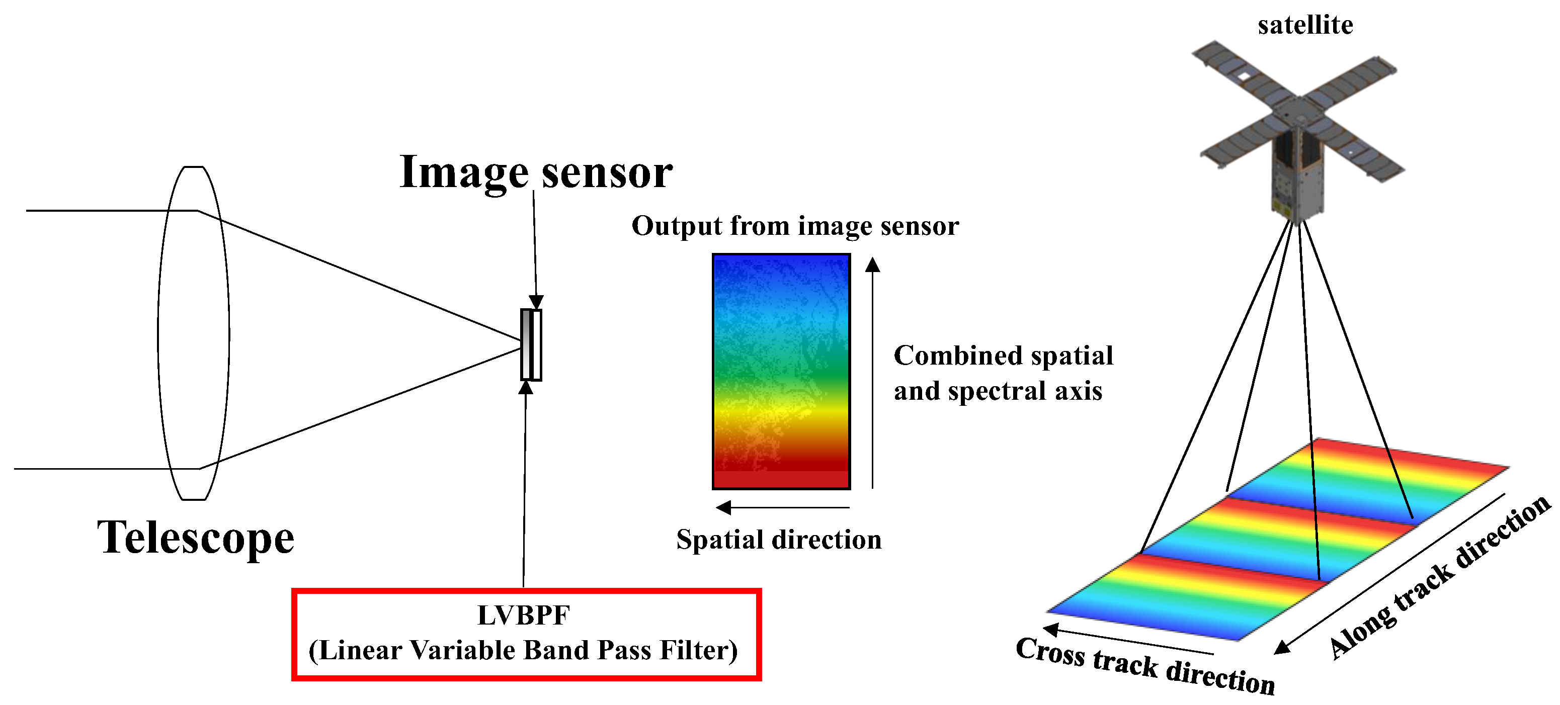
Figure 2.
Exterior view and mechanical configuration of the LVBPF-based hyperspectral camera.
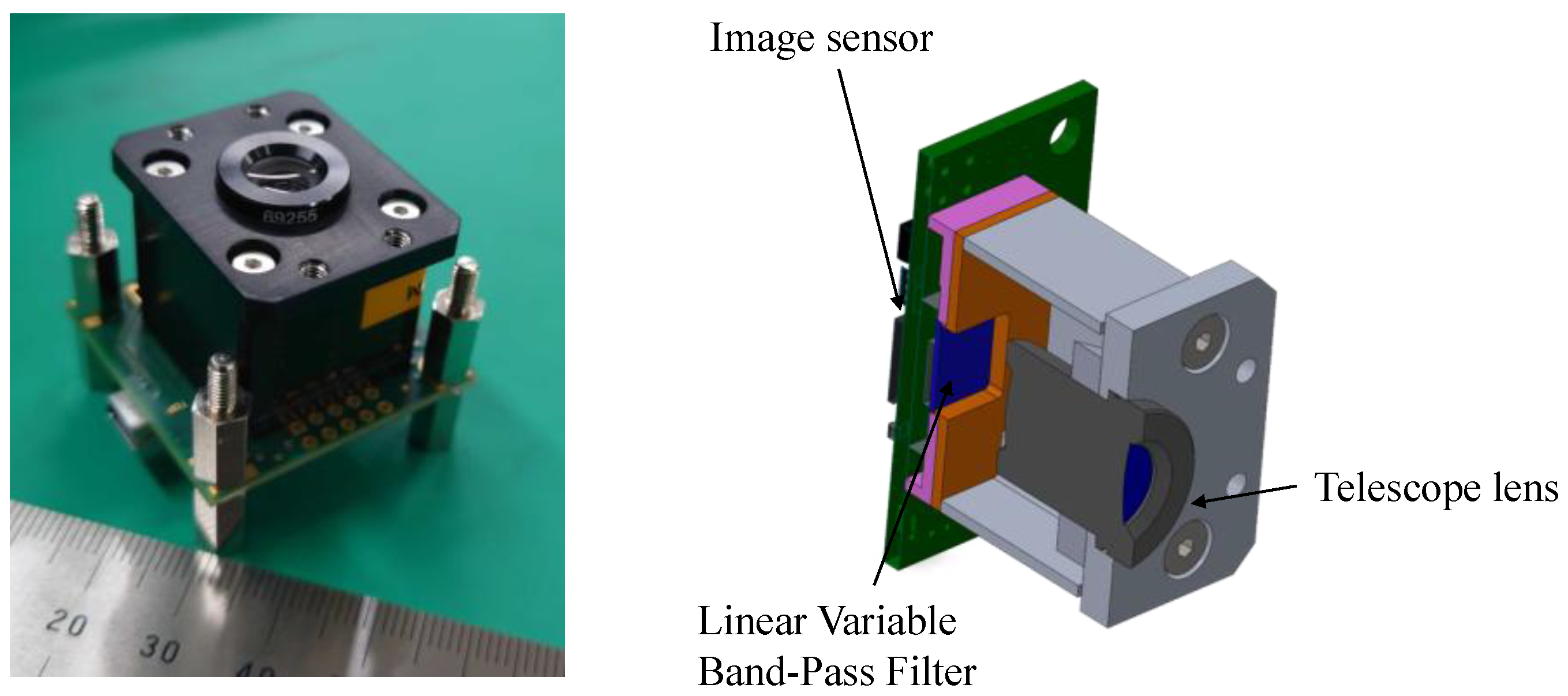
Figure 3.
Point spread function of the hyperspectral camera flight model: (a) before environmental testing; (b) after environmental testing.
Figure 3.
Point spread function of the hyperspectral camera flight model: (a) before environmental testing; (b) after environmental testing.
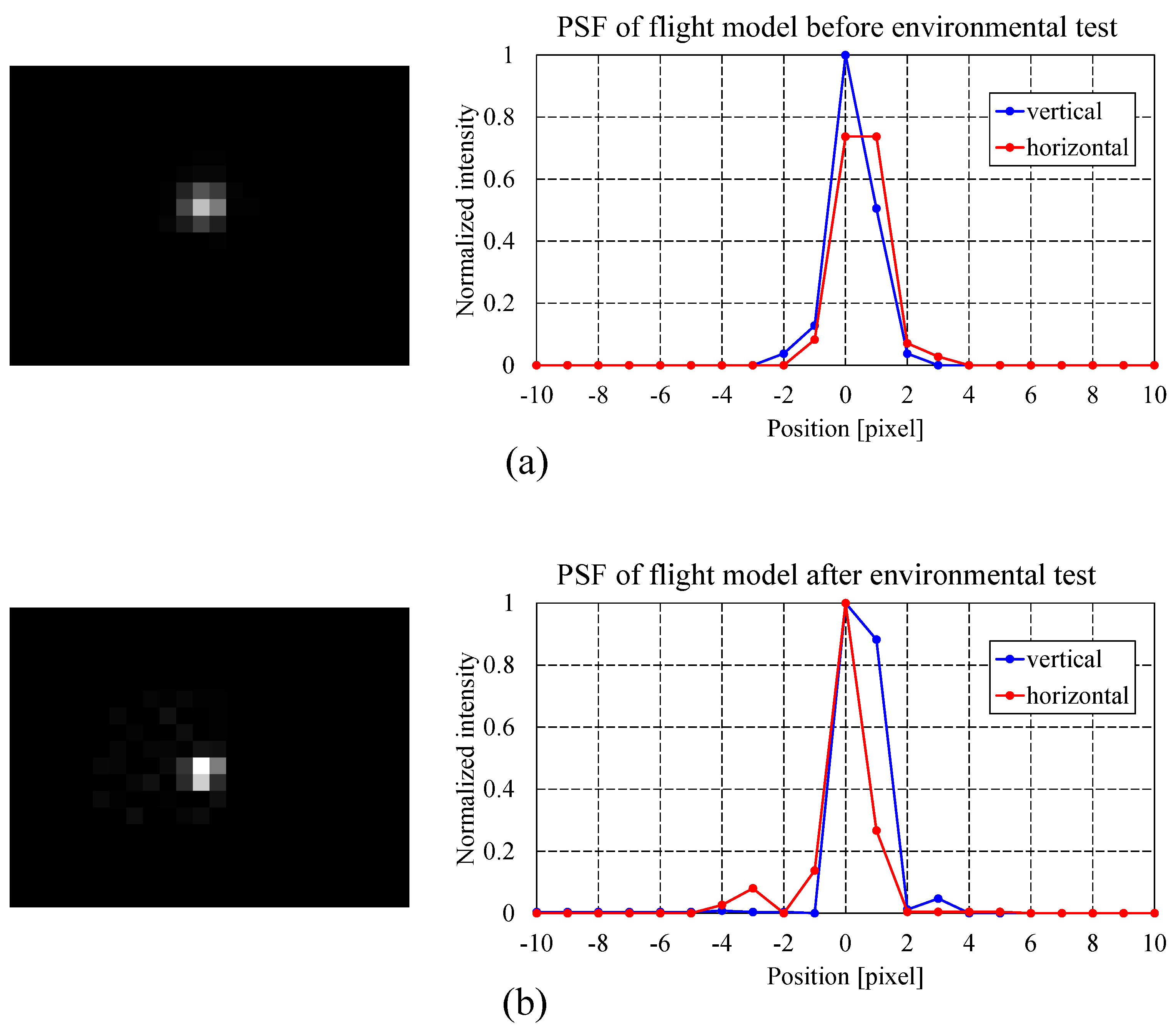
Figure 4.
Spectral image acquired by the hyperspectral camera flight model across spectral bands of (a) 400 nm, (b) 450 nm, (c) 500 nm, (d) 550 nm, (e) 600 nm, (f) 650 nm, and (g) 700 nm.
Figure 4.
Spectral image acquired by the hyperspectral camera flight model across spectral bands of (a) 400 nm, (b) 450 nm, (c) 500 nm, (d) 550 nm, (e) 600 nm, (f) 650 nm, and (g) 700 nm.
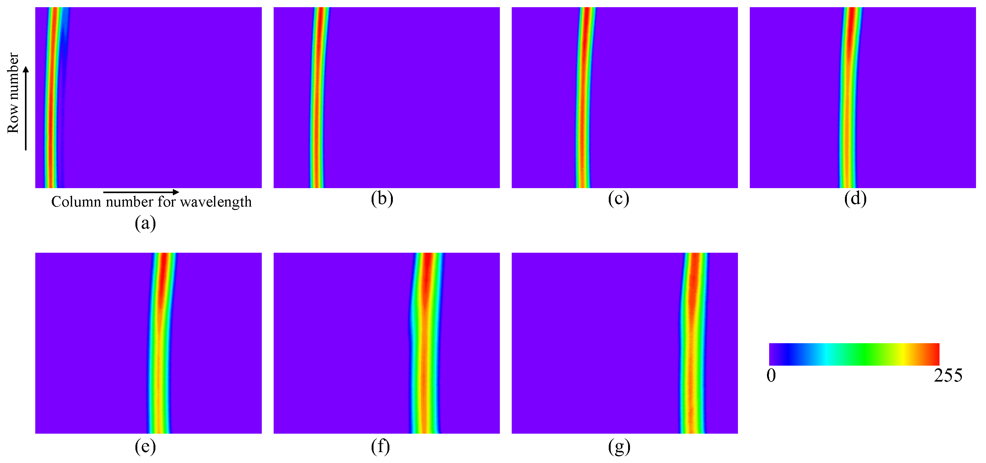
Figure 5.
Smile distortion the hyperspectral camera flight model across spectral bands of (a) 400 nm, 450 nm, 500 nm, and 550 nm, (b) 600 nm, 650 nm, and 700 nm.
Figure 5.
Smile distortion the hyperspectral camera flight model across spectral bands of (a) 400 nm, 450 nm, 500 nm, and 550 nm, (b) 600 nm, 650 nm, and 700 nm.
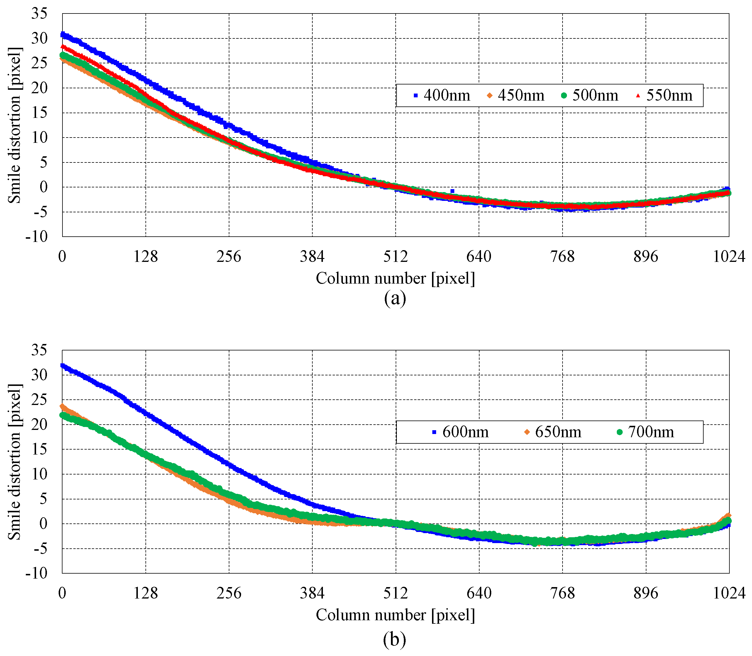
Figure 6.
Calibrated wavelength map of the hyperspectral camera flight model.
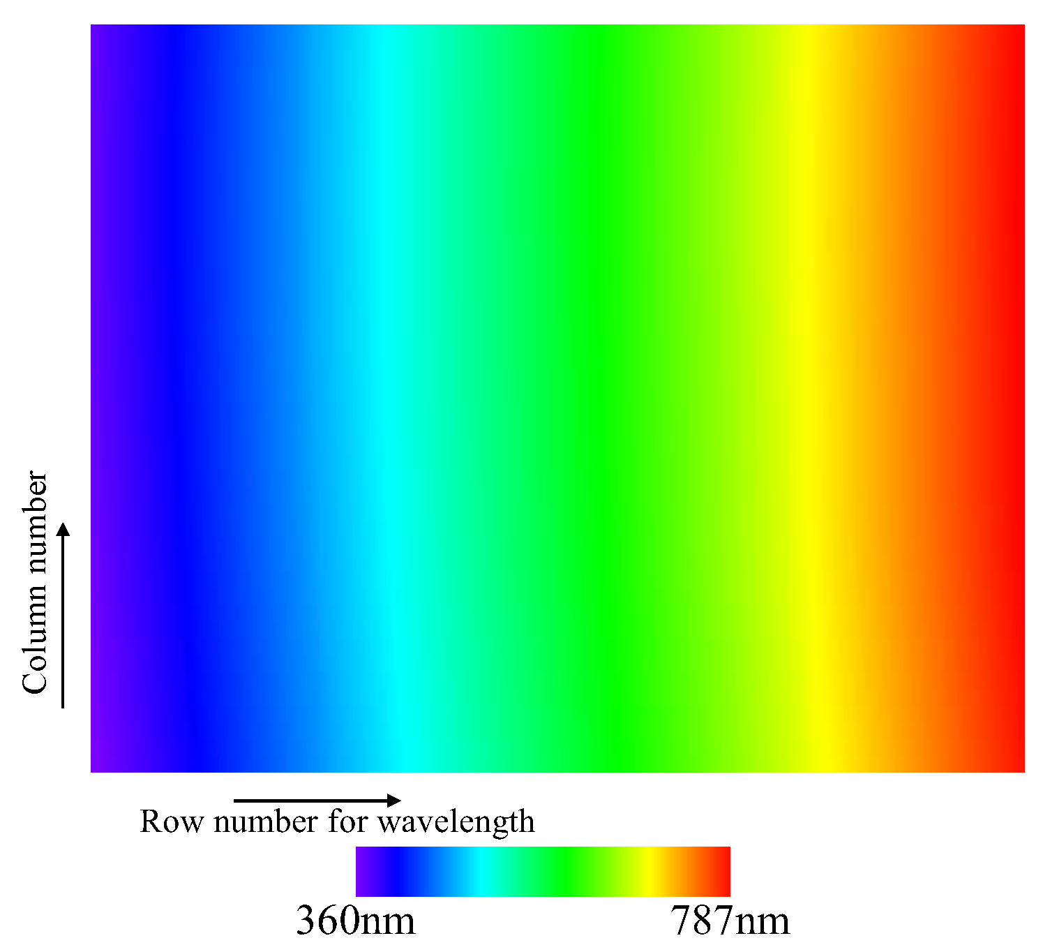
Figure 7.
Spectral resolution of each band in the hyperspectral camera flight model.
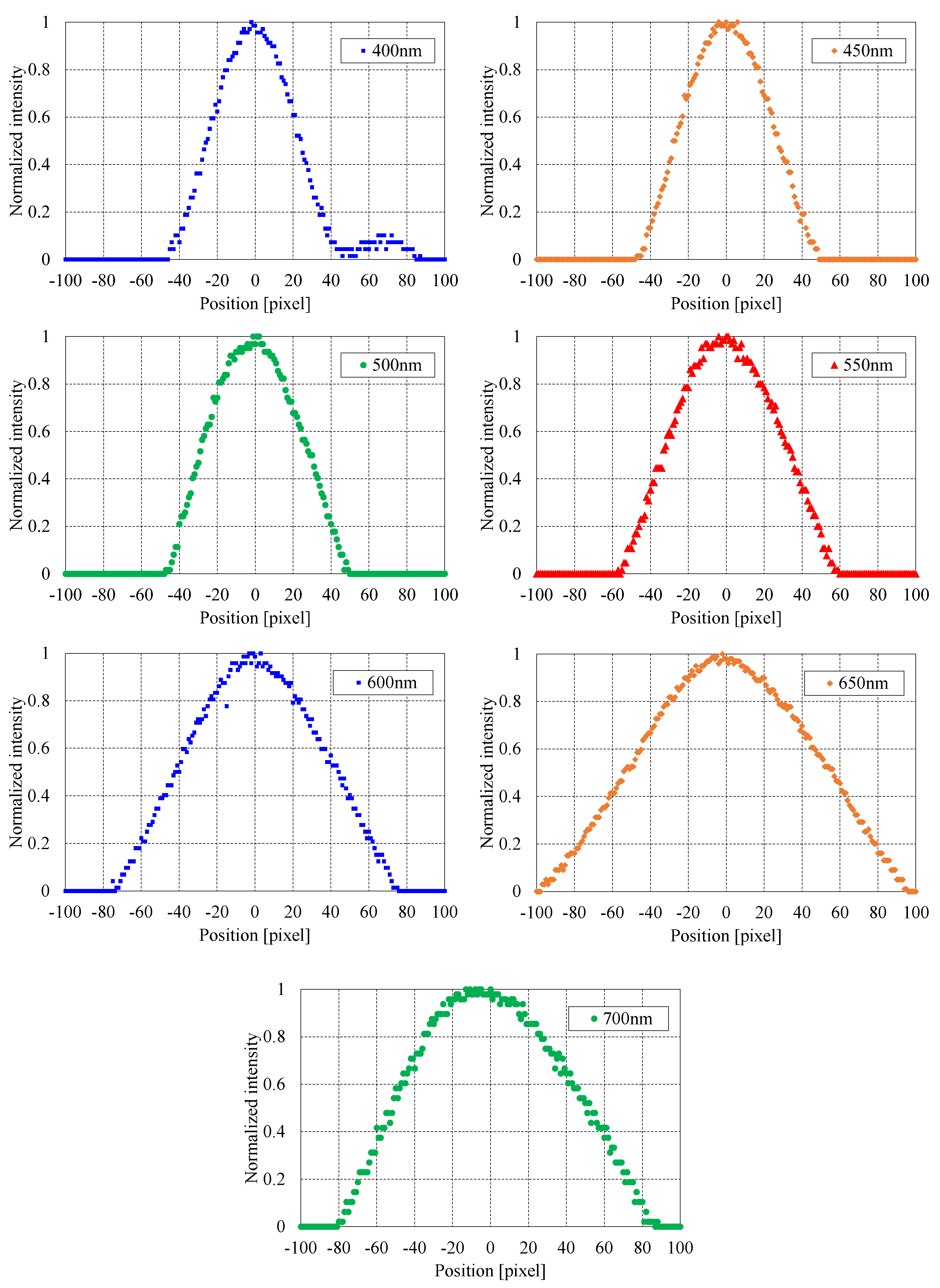
Figure 8.
Flight model of TIRSAT.
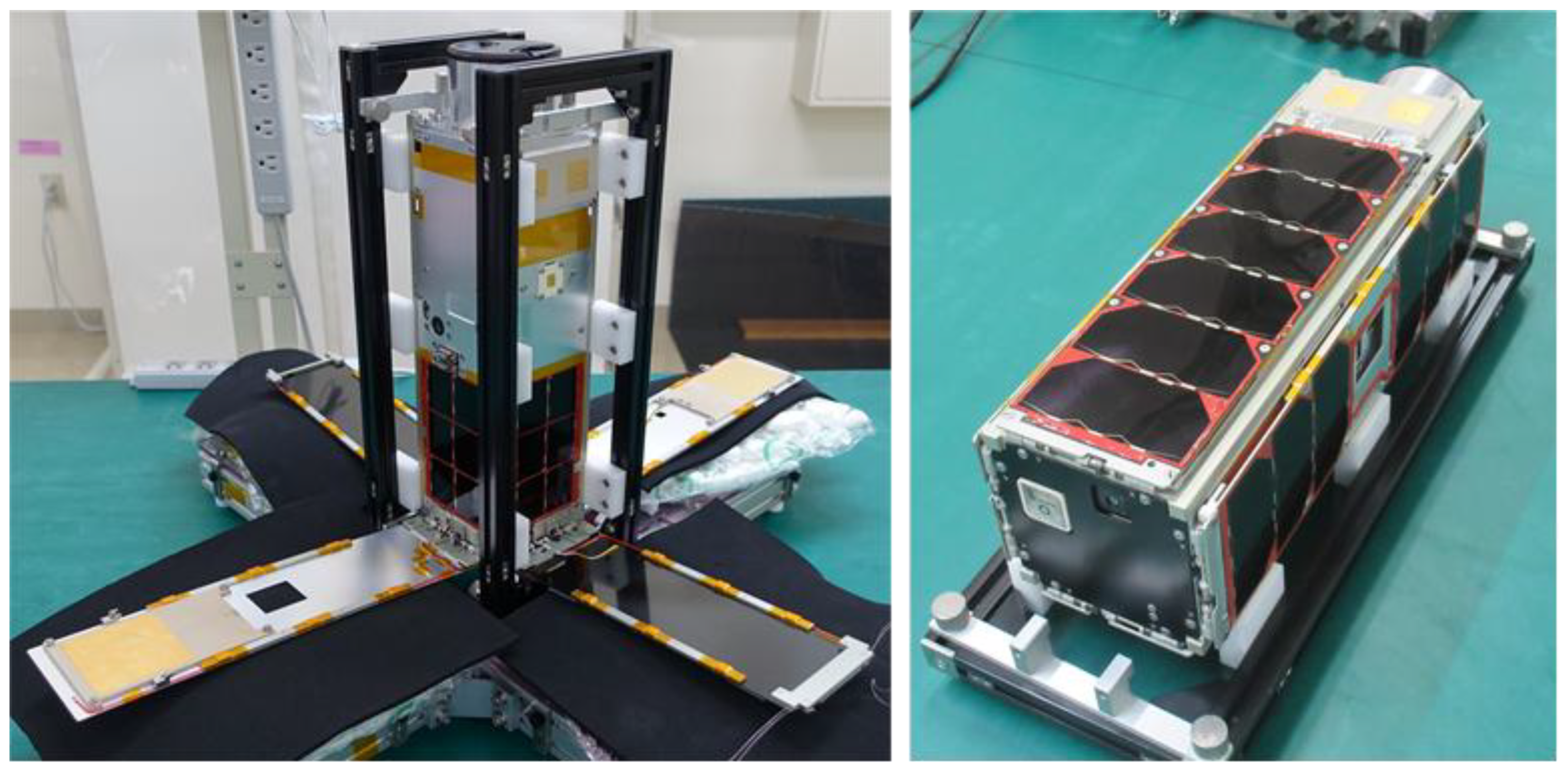
Figure 9.
Mechanical configuration of TIRSAT.
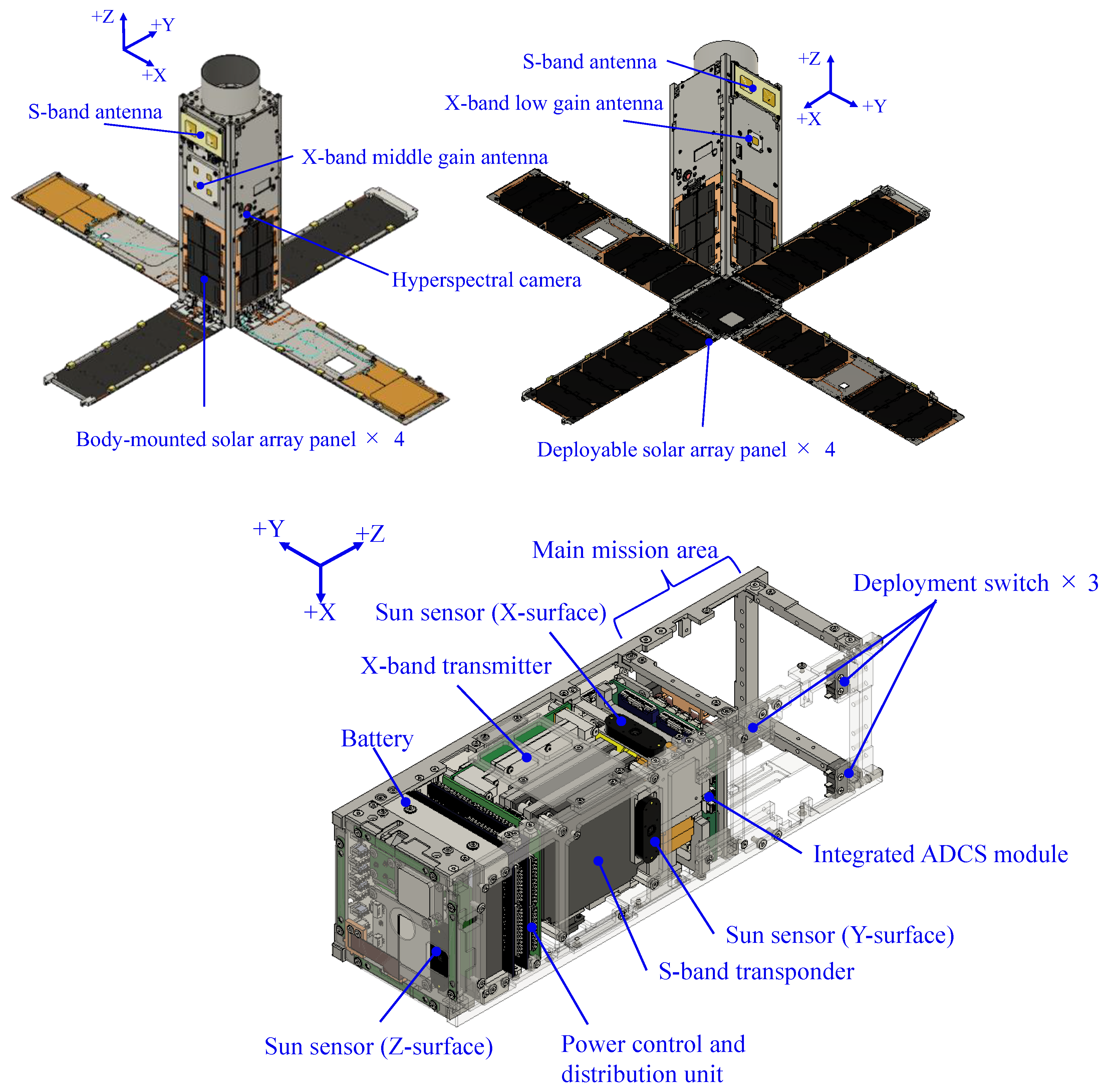
Figure 10.
Configuration of the ADCS onboard TIRSAT.
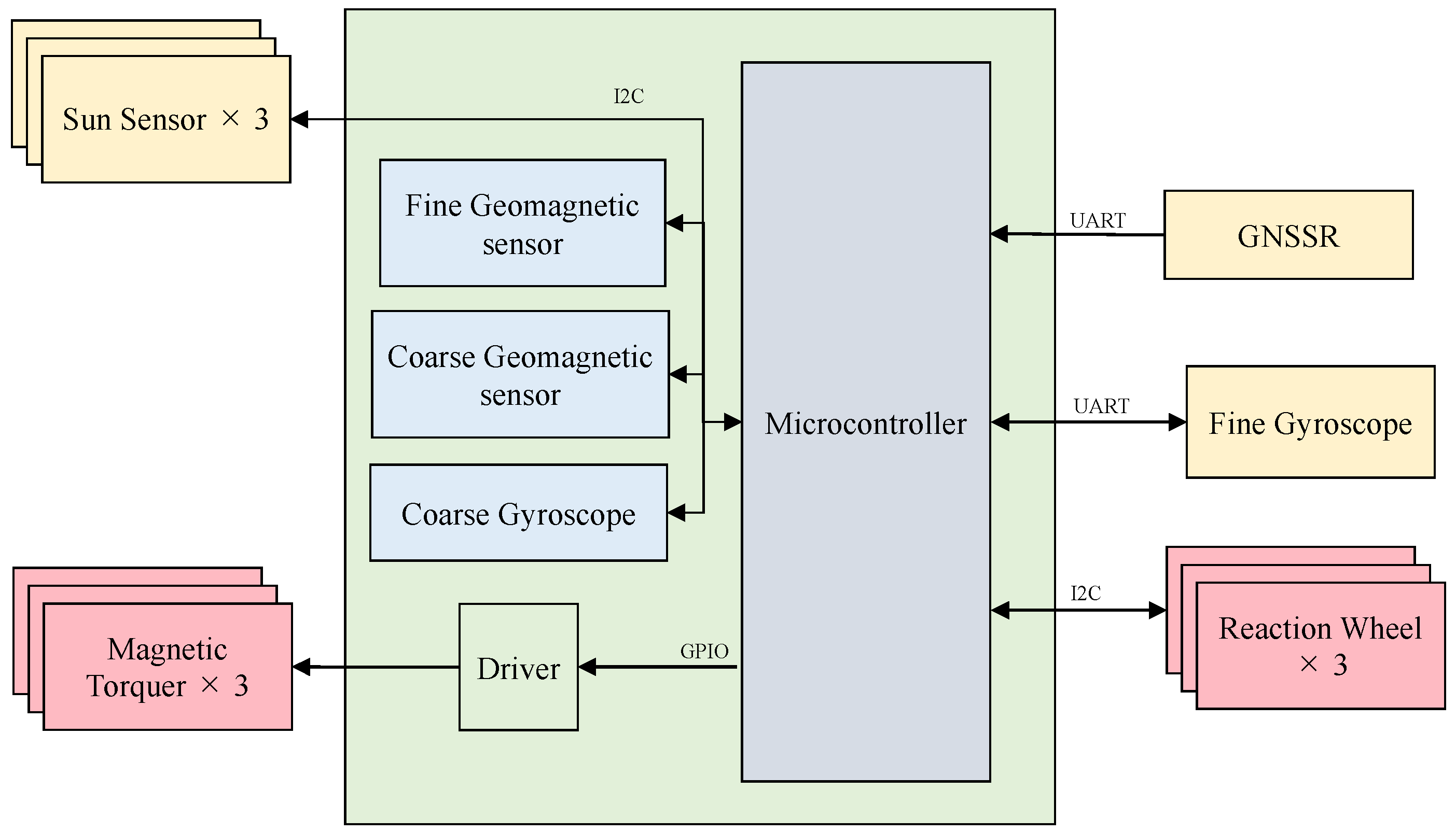
Figure 11.
Simulation results of pointing control error using SILS. Case A: –X surface faces the Sun; Case B: quaternion = [0.5, –0.5, –0.5, 0.5]; Case C: quaternion = [0.5, –0.5, 0.5, –0.5]; Case D: quaternion = [0, 0, 0.707, –0.707]; Case E: quaternion = [0.707, –0.707, 0, 0]. Upper panel: overall results; lower panel: magnified view.
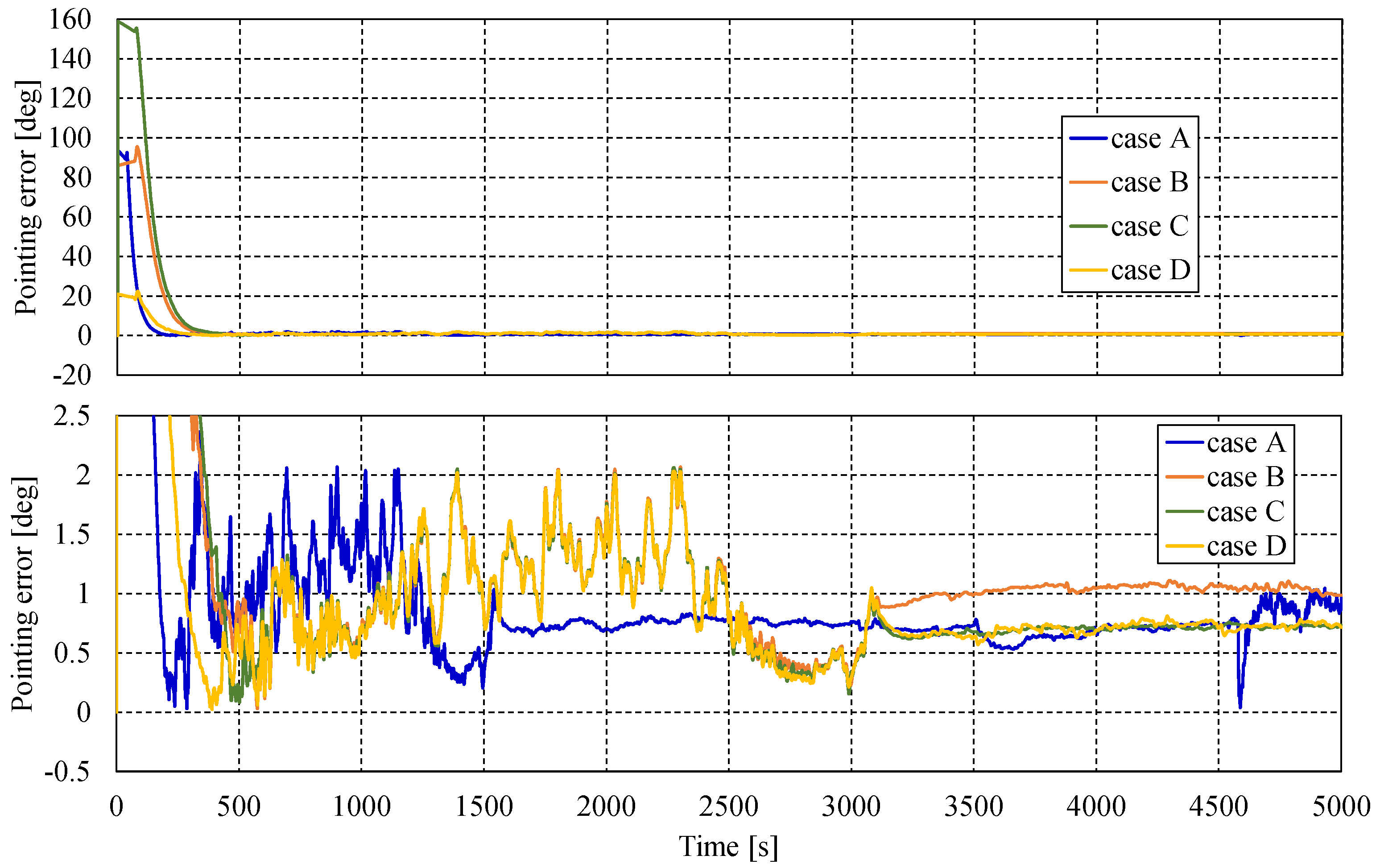
Figure 12.
Schematic of attitude control accuracy and stability concept.
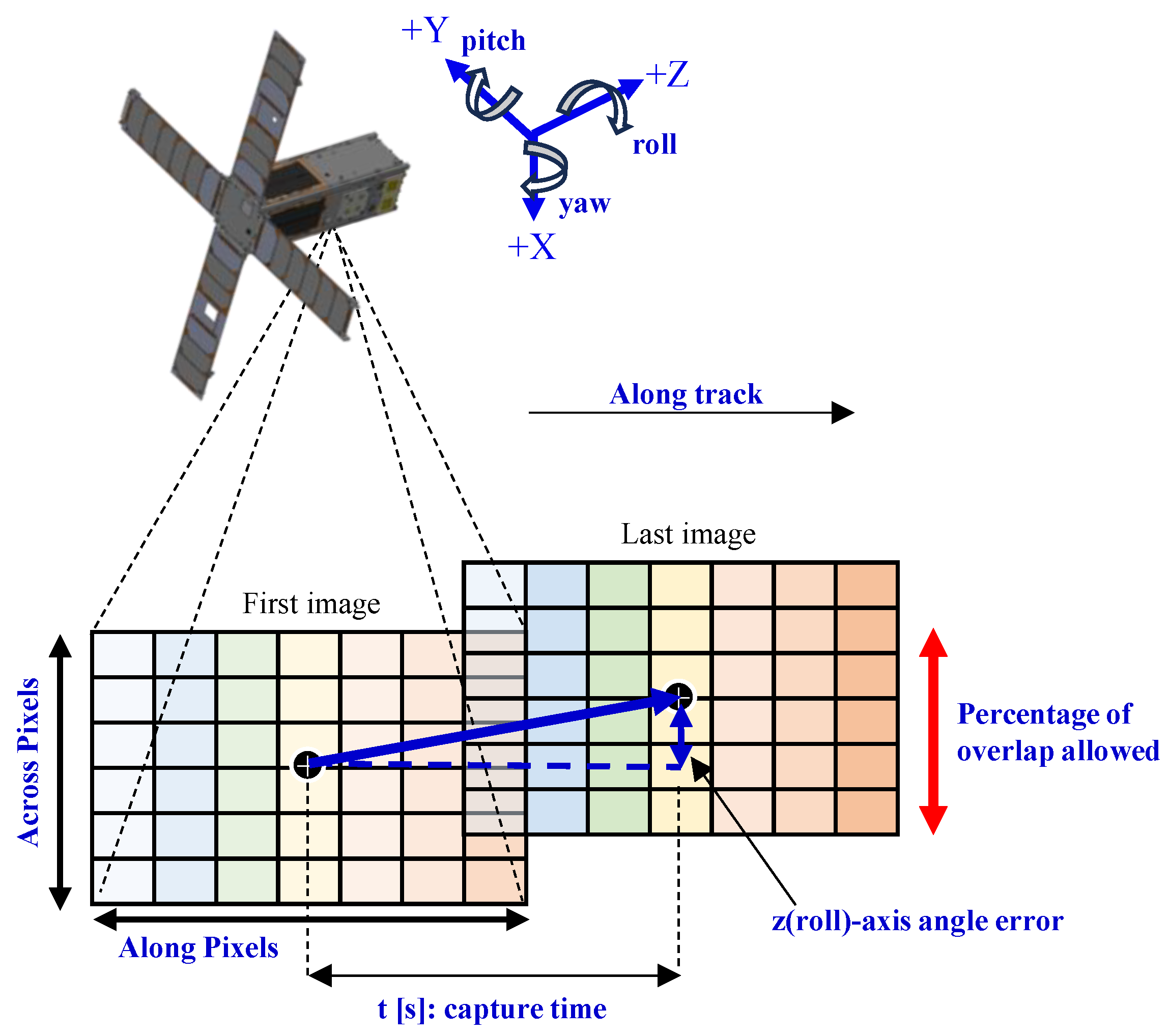
Figure 13.
System block diagram of the mission data handling system and X-band transmitter.
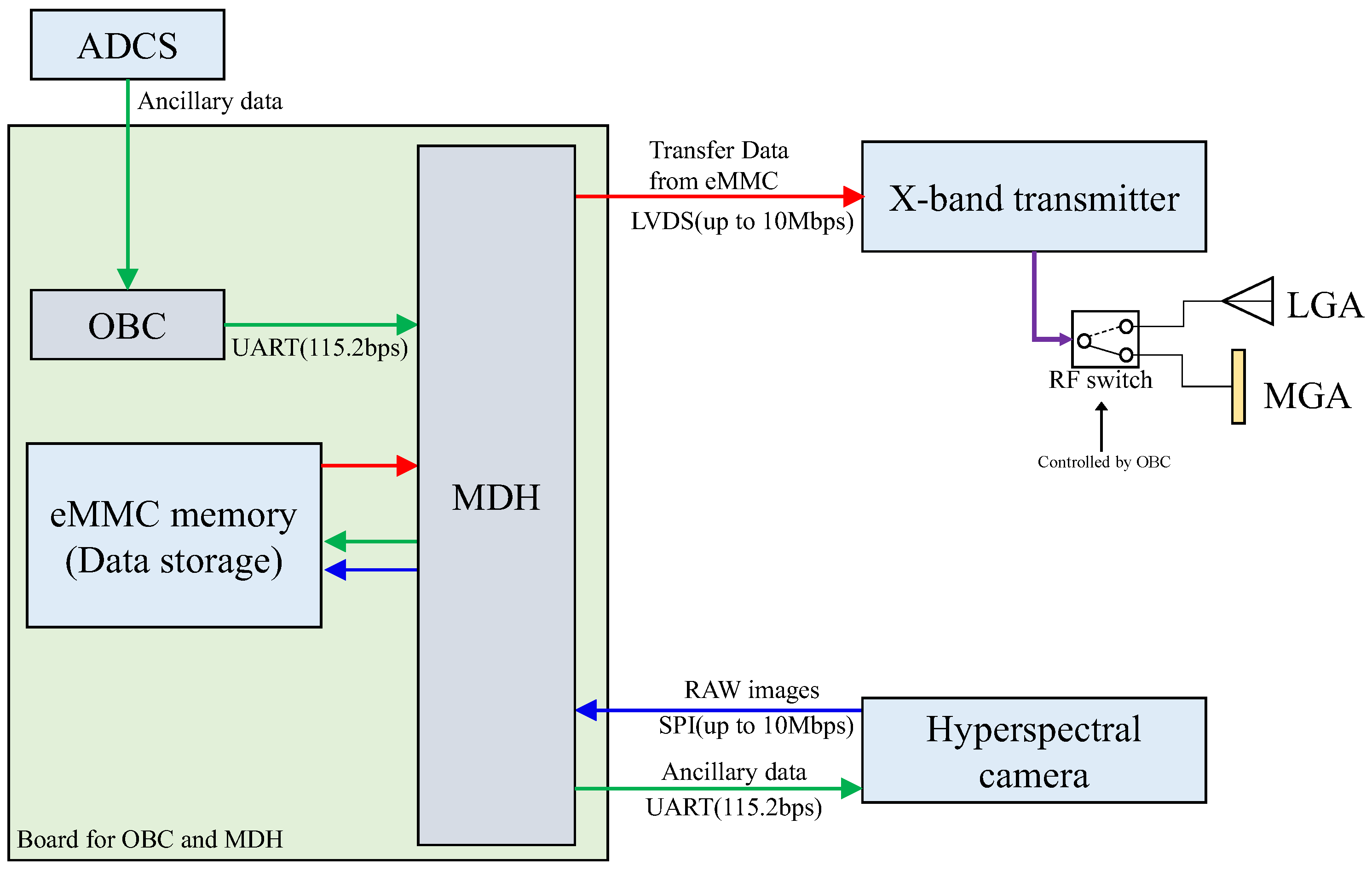
Figure 14.
Data construction procedure for LVBPF-based hyperspectral data.
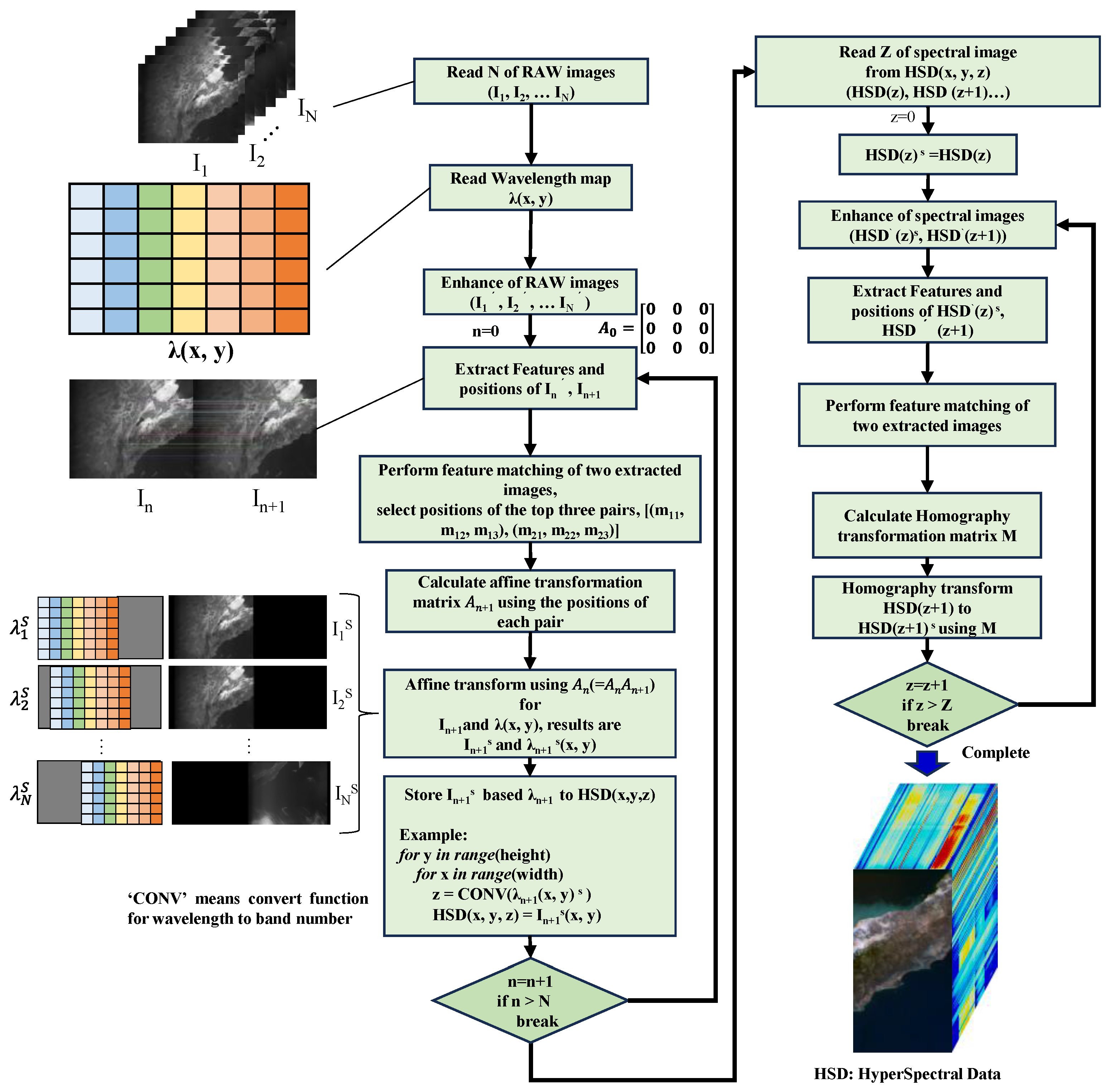
Figure 15.
Composite image (467 nm, 547 nm, and 637 nm) and corresponding spectral data at locations A, B, C, and D (2024-11-14 17:34:12 UTC, Baja California, Mexico).
Figure 15.
Composite image (467 nm, 547 nm, and 637 nm) and corresponding spectral data at locations A, B, C, and D (2024-11-14 17:34:12 UTC, Baja California, Mexico).
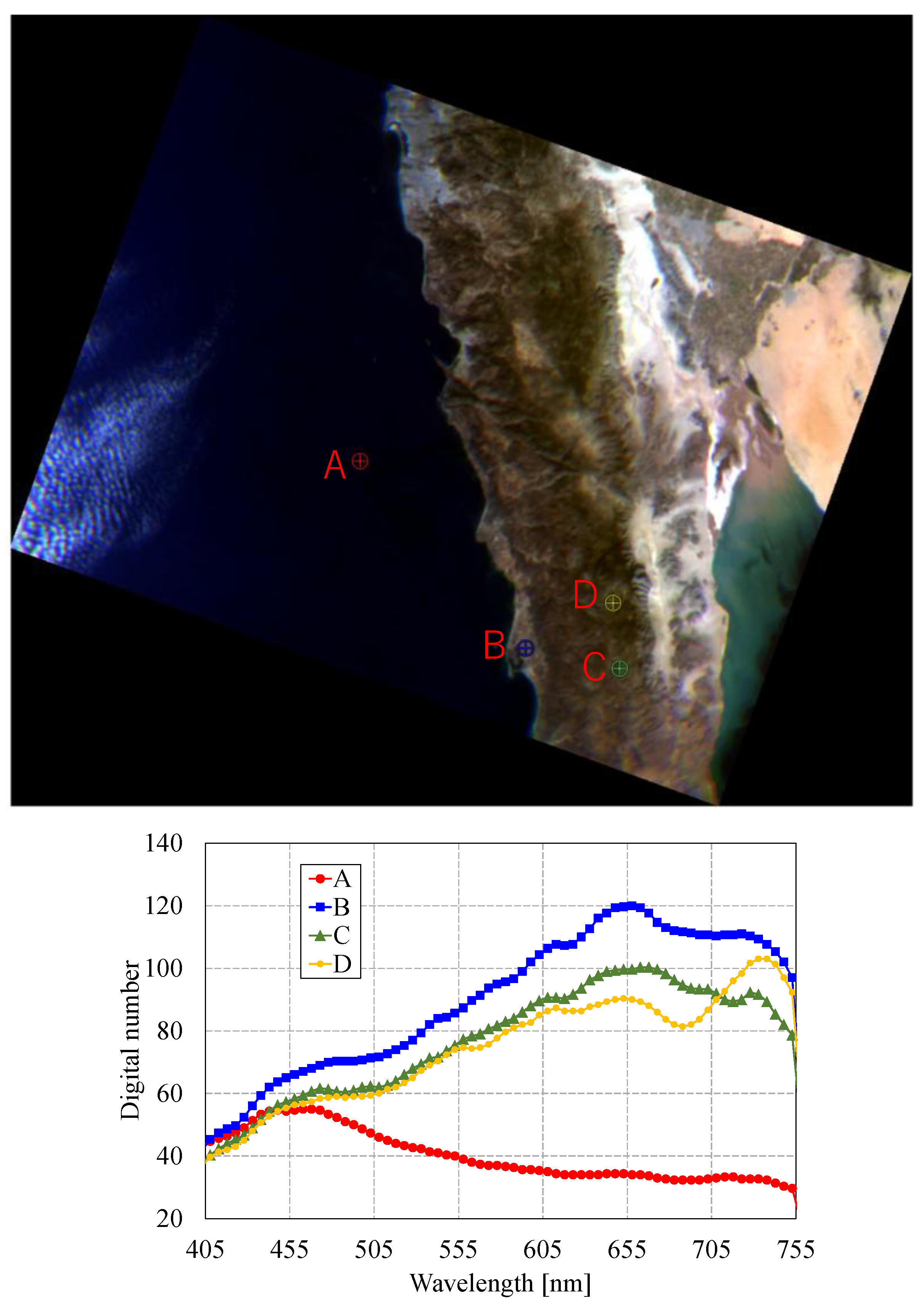
Figure 16.
Composite image (467 nm, 547 nm, and 637 nm) and corresponding spectral data at locations A, B, C, and D (2024-09-09 08:04:59 UTC, from Romania to Bulgaria).
Figure 16.
Composite image (467 nm, 547 nm, and 637 nm) and corresponding spectral data at locations A, B, C, and D (2024-09-09 08:04:59 UTC, from Romania to Bulgaria).
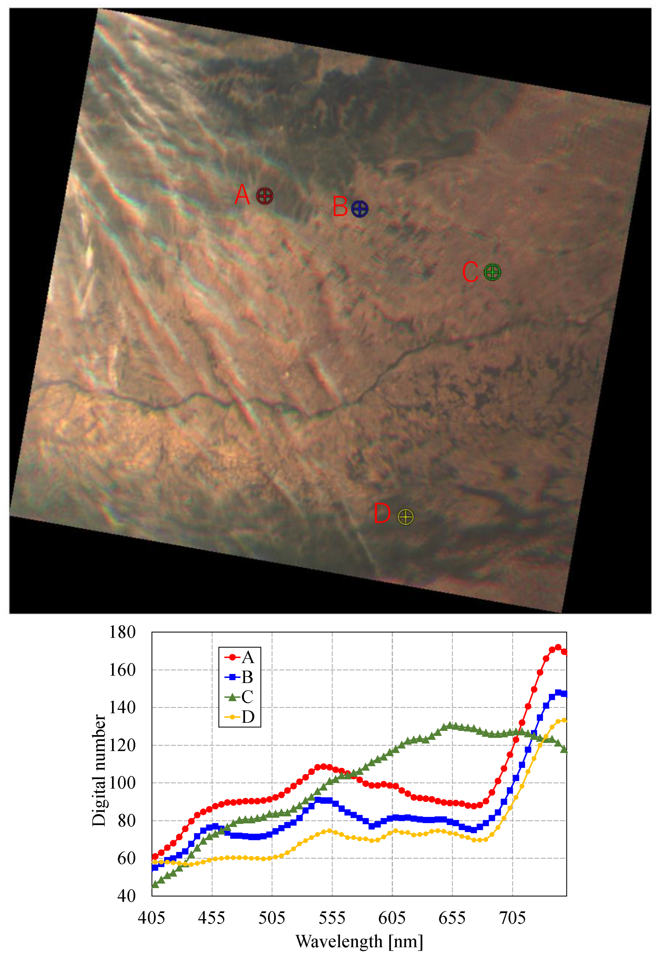
Figure 17.
Composite image (467 nm, 547 nm, and 742 nm) and corresponding spectral data at locations A, B, C, and D (2025-01-08 17:30:12 UTC, near Nevada, USA).
Figure 17.
Composite image (467 nm, 547 nm, and 742 nm) and corresponding spectral data at locations A, B, C, and D (2025-01-08 17:30:12 UTC, near Nevada, USA).
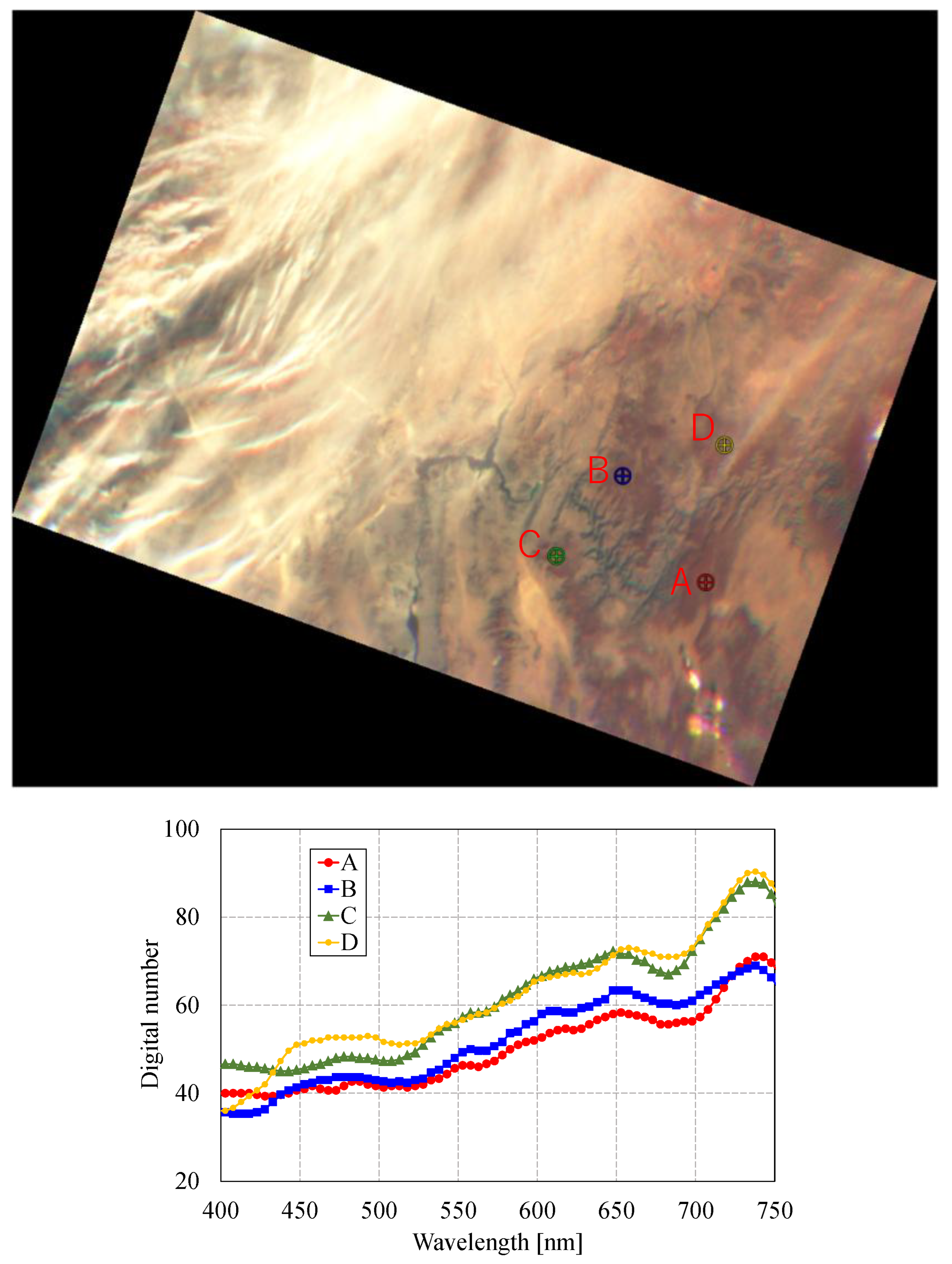
Figure 18.
Positional shifts from data construction methods: (1) Sequential synthesis; (2) Affine; (3) Homography; (4) Proposed method. Composite image at 467 nm, 547 nm, and 637 nm (2024-12-16 05:55:12 UTC, Kazakhstan).
Figure 18.
Positional shifts from data construction methods: (1) Sequential synthesis; (2) Affine; (3) Homography; (4) Proposed method. Composite image at 467 nm, 547 nm, and 637 nm (2024-12-16 05:55:12 UTC, Kazakhstan).
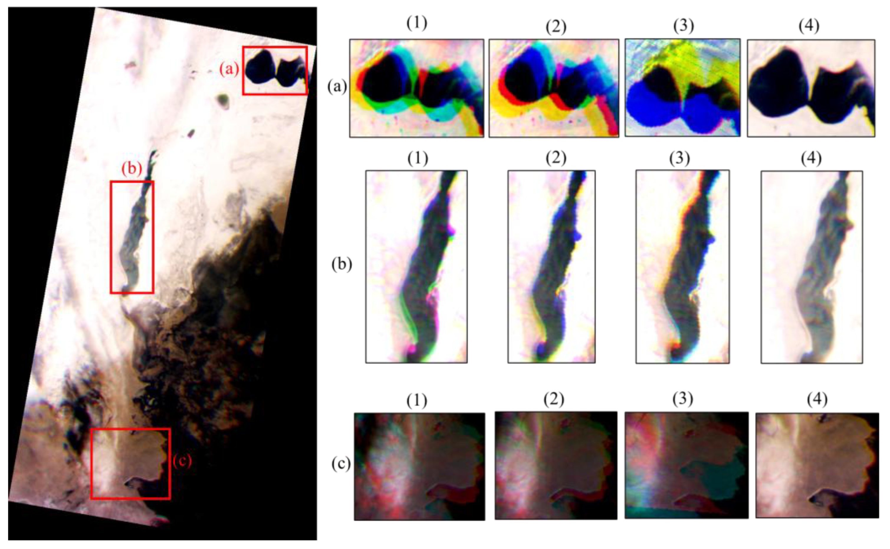
Figure 19.
Geometric correction comparison: (a) RAW image by TIRSAT/hyperspectral camera (2025-01-14 17:16:47 UTC); (b) image by Landsat-9 OLI-2 (2025-03-30 18:10:25 UTC).
Figure 19.
Geometric correction comparison: (a) RAW image by TIRSAT/hyperspectral camera (2025-01-14 17:16:47 UTC); (b) image by Landsat-9 OLI-2 (2025-03-30 18:10:25 UTC).
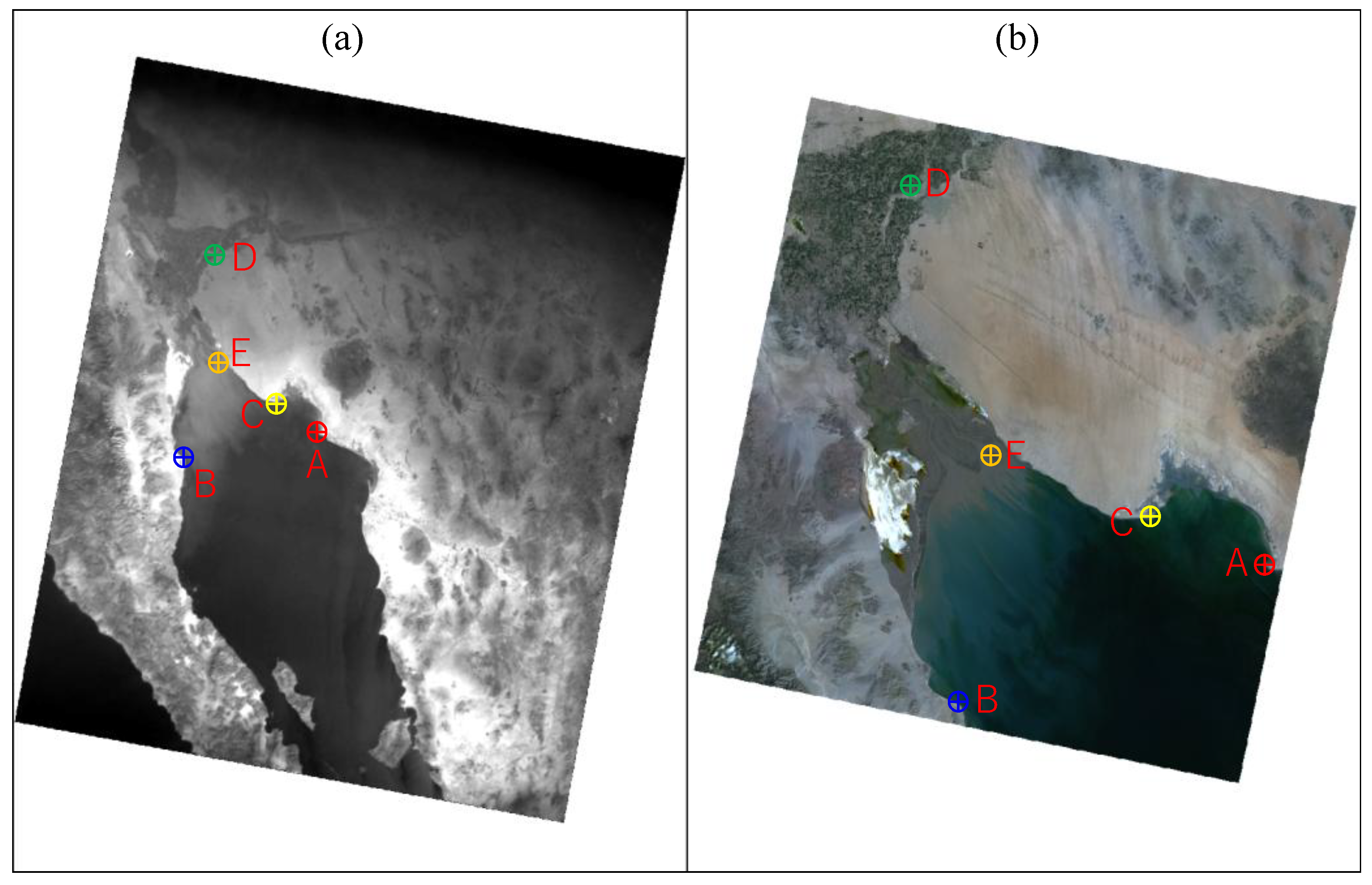
Figure 20.
Angular velocity history during TIRSAT imaging (2025-01-14 17:16:47 UTC). Upper panel: overall results; lower panel: roll-axis close-up.
Figure 20.
Angular velocity history during TIRSAT imaging (2025-01-14 17:16:47 UTC). Upper panel: overall results; lower panel: roll-axis close-up.
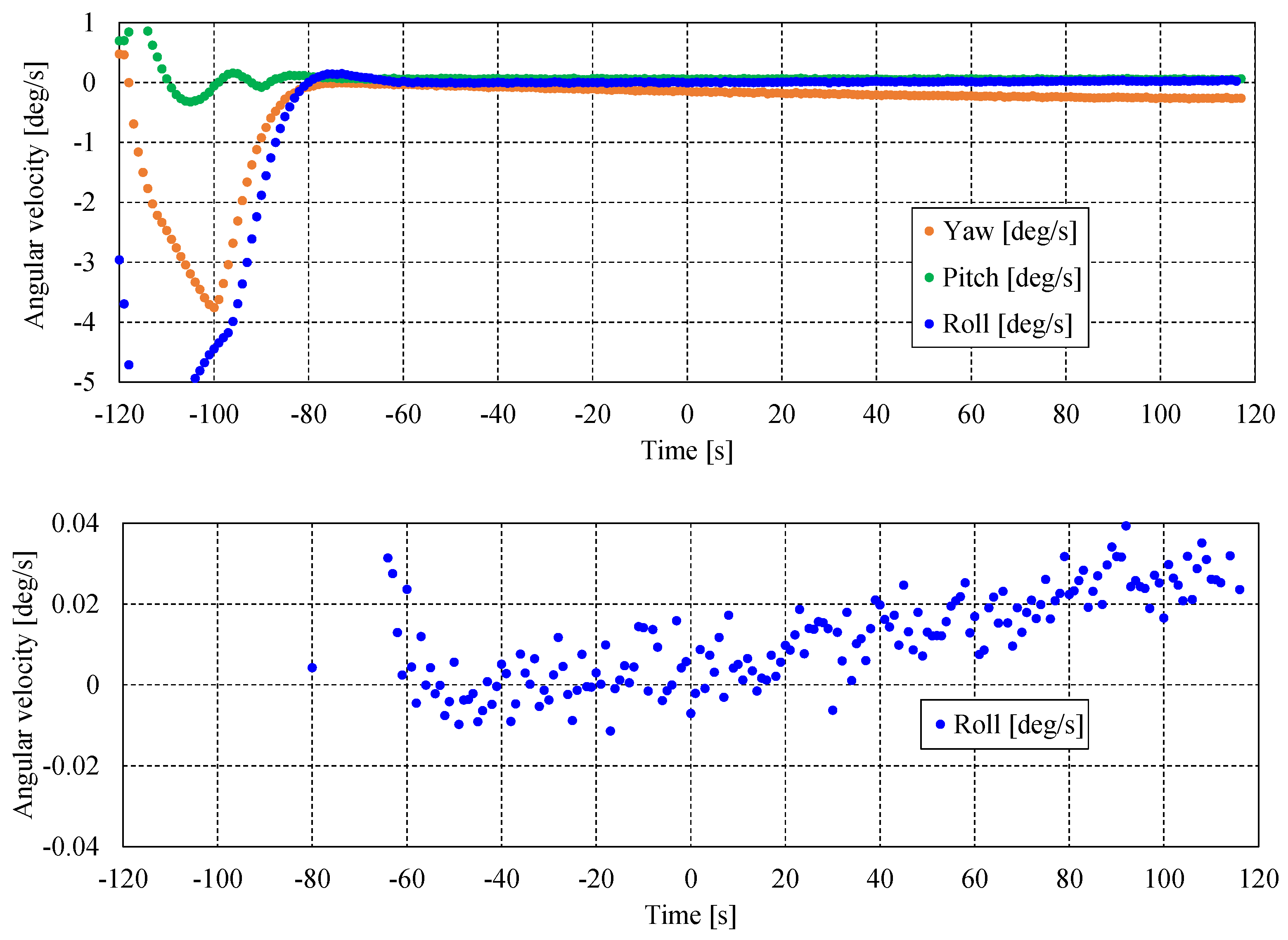
Figure 21.
Comparison of simulated and on-orbit measured temperatures.
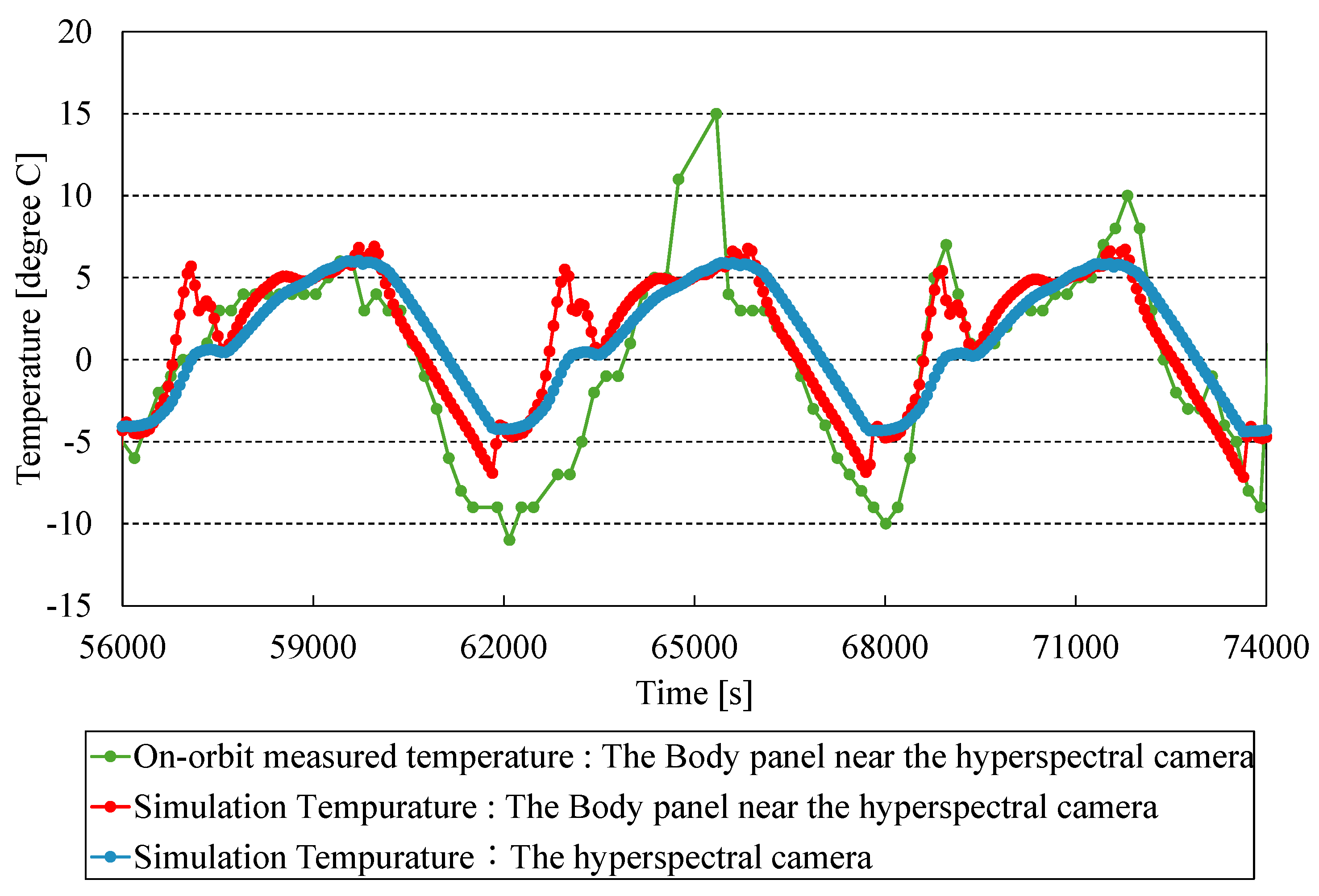
Figure 22.
Power generation after deployment of solar panels.
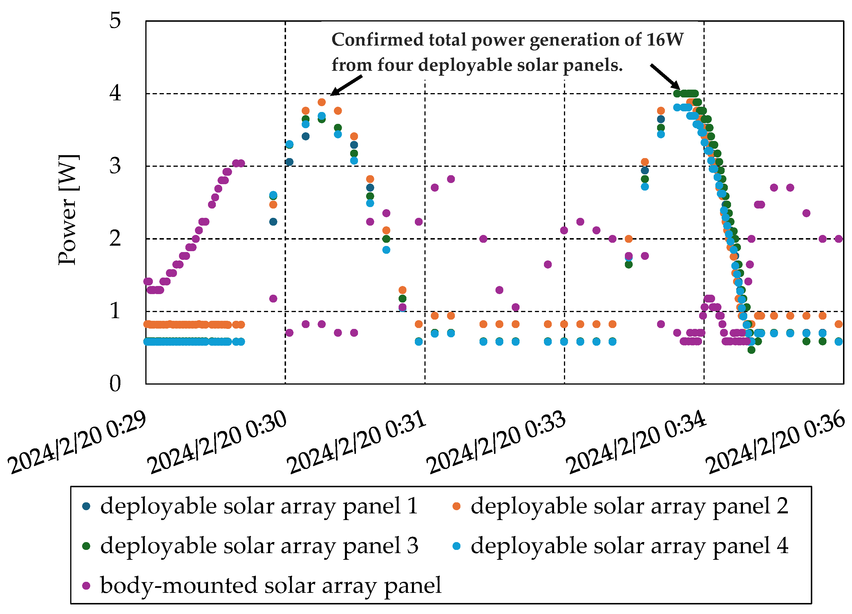
Figure 23.
Power generation after deployment of solar panels.
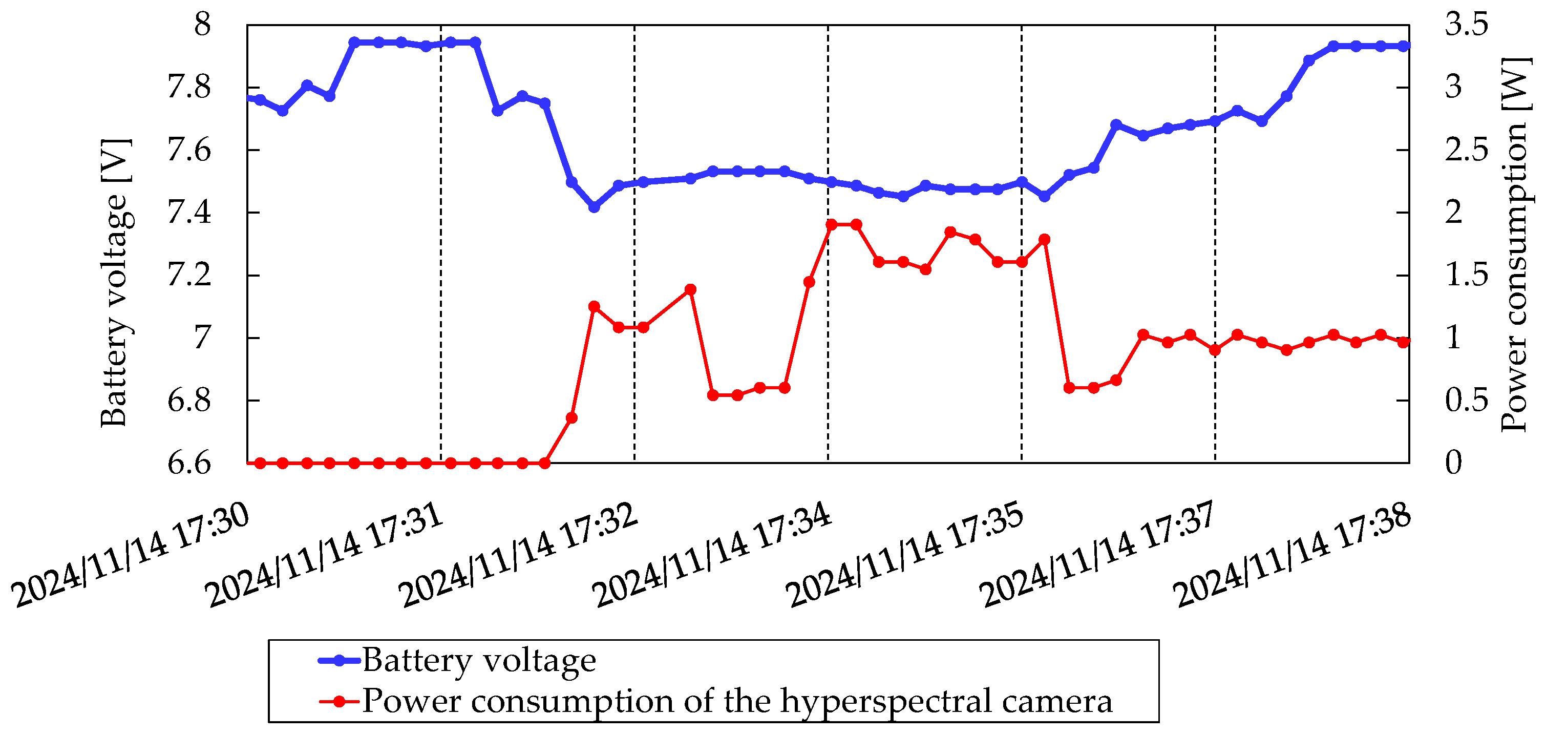
Figure 24.
Power generation after deployment of solar panels.
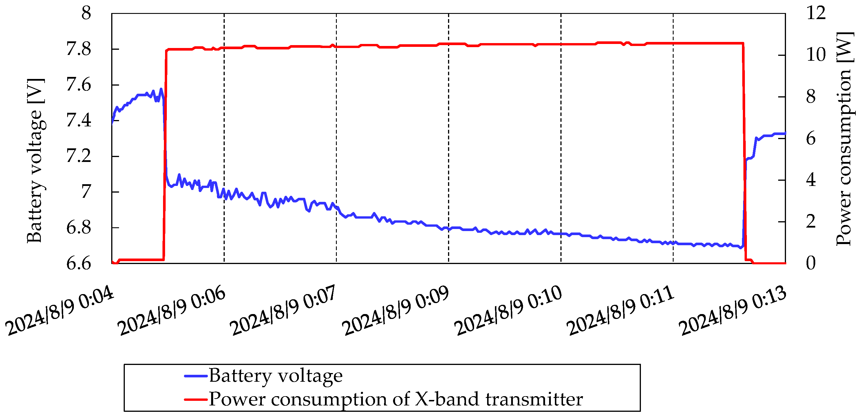
Figure 25.
Comparison of hyperspectral data from two dates: (a) 2024-11-14 17:34:12 UTC; (b) 2025-01-14 17:16:12 UTC.
Figure 25.
Comparison of hyperspectral data from two dates: (a) 2024-11-14 17:34:12 UTC; (b) 2025-01-14 17:16:12 UTC.

Figure 26.
Spectral data comparison across time at each location: A, B (vegetation in mountainous region); C, D (intermountain region); E, F (coastal region).
Figure 26.
Spectral data comparison across time at each location: A, B (vegetation in mountainous region); C, D (intermountain region); E, F (coastal region).
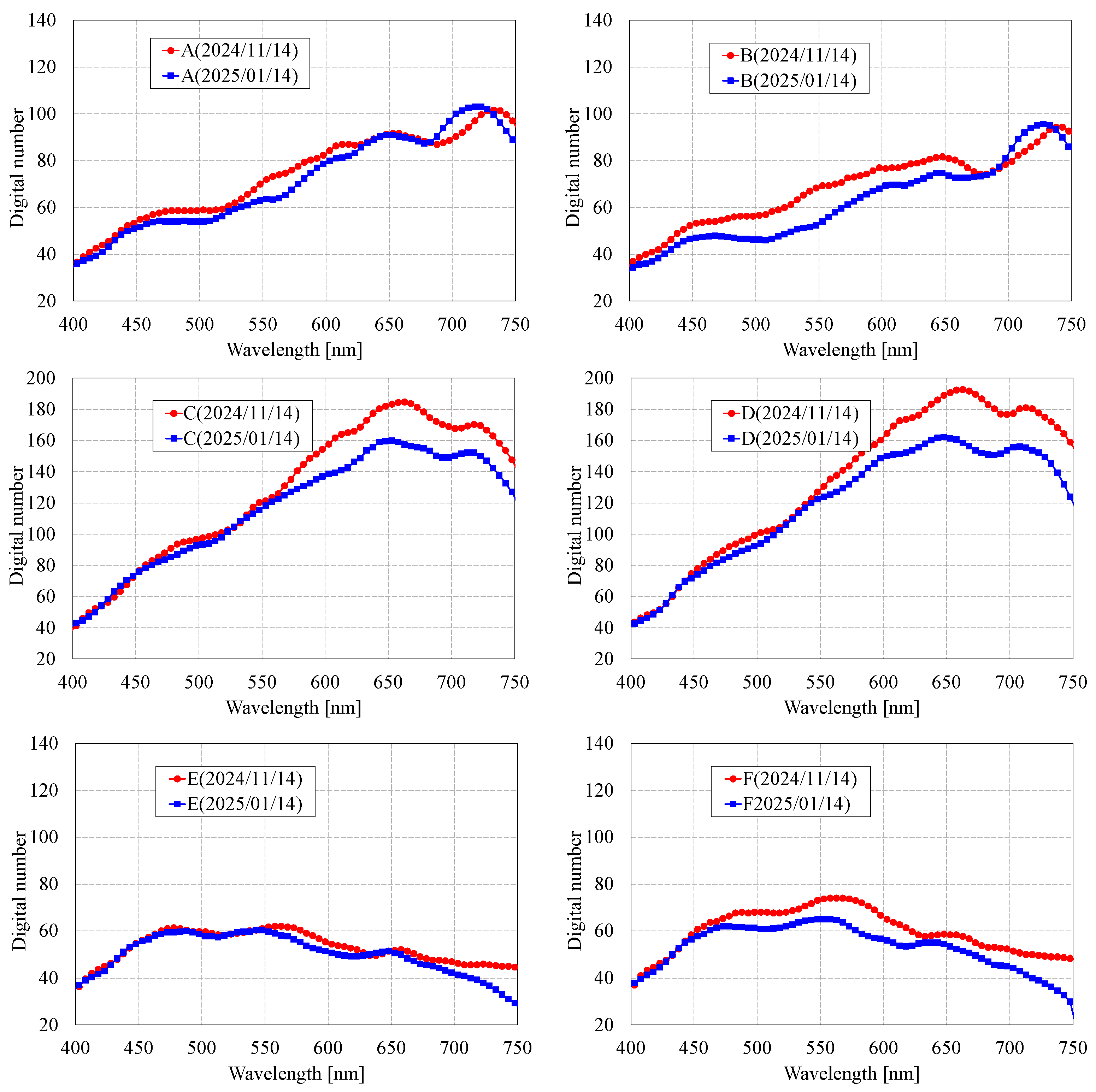
Figure 27.
Comparison of GNDVI from two time periods.
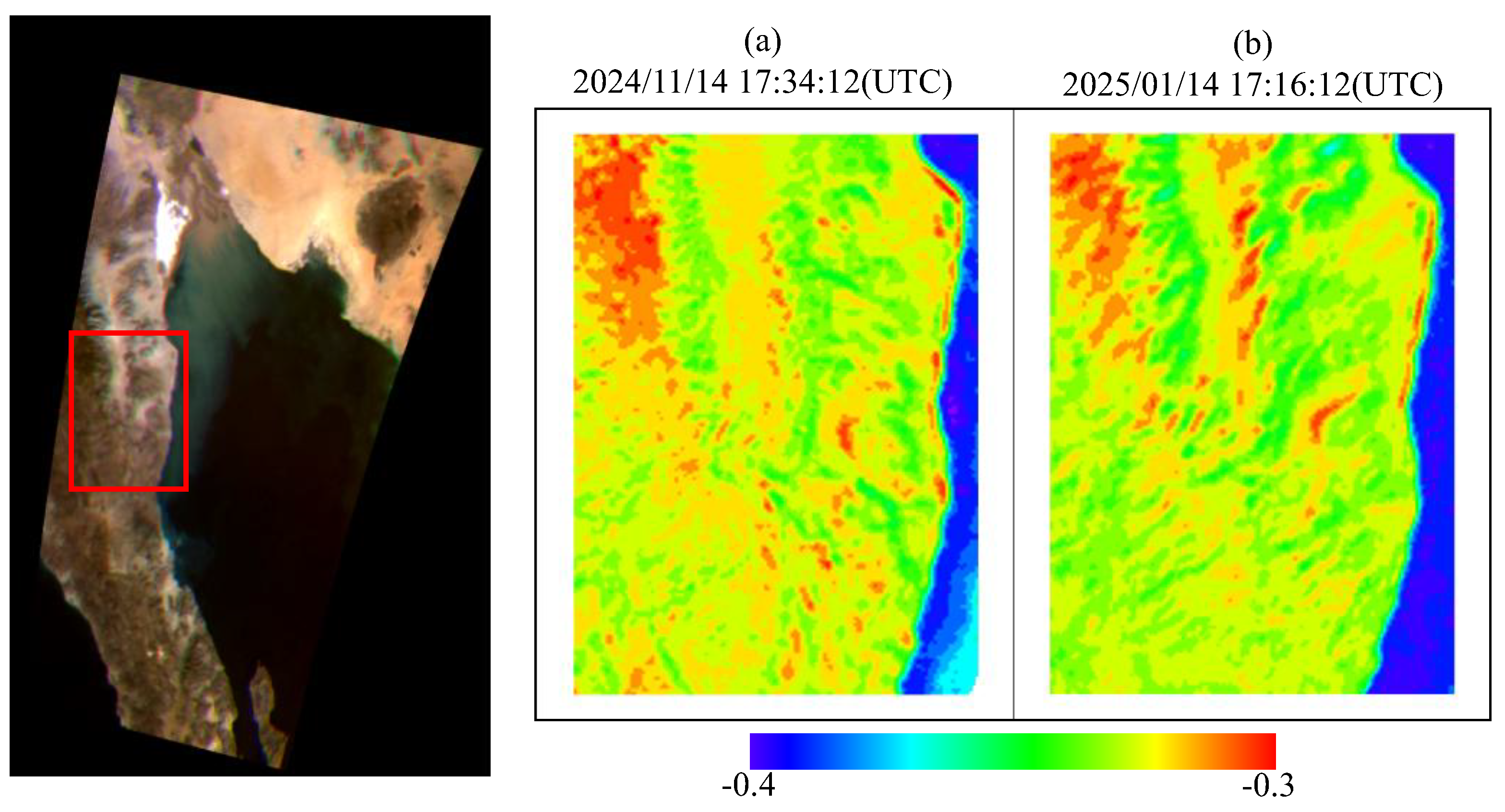

Table 1.
Specifications of the developed hyperspectral camera.
| Item | Specification |
|---|---|
| Size | 3.6 cm x 3.6 cm x 2.4 cm |
| Weight | 35 g |
| Ground sampling distance | 450 m/pixel |
| Swath | 460 km |
| Available wavelength range | 400 nm – 770 nm |
| Spectral sampling distance | 5 nm |
| Spectral resolution | 18.5 nm |
| Number of Band | 75 band |
| Focal length of telescope lens | 8 mm |
| F-number of telescope lens | F/2.5 |
| Valid pixel area | 1280 x 1024 pixels |
| Pixel size | 5.3 μm |
| Dynamic range | 8 bit |
Table 2.
Specifications of the LVBPF.
| Item | Specification |
|---|---|
| Size | 10.1 mm x 8 mm |
| Thickness | 0.5 mm |
| Valid wavelength range | 380–850 nm |
| Dispersion | 67.7 nm/mm |
| Peak transmission | 65% |
| Spectral blocking property | < 1% |
| Half bandwidth | 15 nm at 430 nm20.6 nm at 780 nm |
Table 3.
Specifications of the TIRSAT satellite bus.
| Item | Specification |
|---|---|
| Size | 117 mm x 117 mm x 381 mm |
| Weight | 4.97 kg |
| Attitude Determination and Control Subsystem | 3-axis stabilization control using geomagnetic sensor, MEMS gyroscope, 3-sun sensor, GPS receiver, magnetic torque, and reaction wheel |
| Electrical Power Subsystem | Solar array panel: 4 deployable panels, 4 body-mounted panels Maximum power generation: 20 W Typical power consumption: 10 W Battery: 5.8 Ah, Nominal 8 V (Lithium-ion battery) |
| Communication Subsystem | Telemetry/Command: S-band Command Uplink: 4 kbps, Telemetry Downlink: 4 kbps – 64 kbps Mission data downlink: X-band (5 Mbps, 10 Mbps) |
| Orbit | Sun-synchronous sub-recurrent orbit Altitude: 680 km (approximately), Inclination: 98 degrees |
Table 4.
Specifications of the ADCS onboard TIRSAT.
| Item | Specification |
|---|---|
| Reaction wheel | 3-axis mounted Max angular momentum: 3mNms (nominal) 5mNms(peak) |
| Magnetic torquer | 3-axis mounted Magnetic moment: 0.35Am2 |
| Sun sensor | 3-surface mounted accuracy <= 0.5°(3σ) |
| Fine Geomagnetic sensor | Resolution: 13nT |
| Fine Gyroscope | Random noise: 4.36E-05 rad/s(1σ) |
| Microcontroller | Clock: 80MHz, ROM: 512 kiB, RAM: 128KiB |
Table 5.
Required attitude control accuracy and stability for the ADCS.
| Item | Attitude control accuracy (roll, pitch) |
Attitude control accuracy (yaw) |
Attitude stability (roll) |
|---|---|---|---|
| requirements | 7.3° | 5.8° | 0.048°/s |
Table 6.
Parameters for each hyperspectral data construction method.
| Item | (1) Sequentially synthesize |
(2) Affine |
(3) Homography |
(4) Proposed method |
|---|---|---|---|---|
| Image Enhancement | - | Gamma correction (gamma=2.0) | ||
| Unsharp masking | ||||
| Feature detection |
AKAZE | |||
| Transformation | Affine | Homography and RANSAC | (1) + (2) | |
| Library | OpenCV, pillow | |||
Table 7.
Geo-referenced coordinates of satellite images and geometric correction error distances.
| Location | TIRSAT | Landsat-9 | Distance [km] | ||
| Latitude [°] | Longitude [°] | Latitude [°] | Longitude [°] | ||
| A | 31.7117 | -113.8237 | 31.3447 | -113.6420 | 44.297 |
| B | 30.9371 | -114.7187 | 31.4722 | -114.9723 | 64.209 |
| C | 31.4933 | -114.0276 | 31.9123 | -114.1741 | 48.612 |
| D | 33.0178 | -114.7806 | 32.4926 | -114.8430 | 58.692 |
| E | 32.1983 | -114.7021 | 31.6918 | -114.5939 | 57.241 |
Disclaimer/Publisher’s Note: The statements, opinions and data contained in all publications are solely those of the individual author(s) and contributor(s) and not of MDPI and/or the editor(s). MDPI and/or the editor(s) disclaim responsibility for any injury to people or property resulting from any ideas, methods, instructions or products referred to in the content. |
© 2025 by the authors. Licensee MDPI, Basel, Switzerland. This article is an open access article distributed under the terms and conditions of the Creative Commons Attribution (CC BY) license (http://creativecommons.org/licenses/by/4.0/).
Copyright: This open access article is published under a Creative Commons CC BY 4.0 license, which permit the free download, distribution, and reuse, provided that the author and preprint are cited in any reuse.


