Submitted:
13 February 2026
Posted:
13 February 2026
You are already at the latest version
Abstract
This paper addresses distributed formation control for multiple unmanned aerial vehicles (UAVs) operating in obstacle-dense environments under directed switching communication topologies. A leader–follower architecture is adopted, wherein the leader performs online trajectory replanning while followers rely on delayed and intermittently available neighbor information. To simultaneously tackle collision avoidance, formation feasibility under narrow passages, and communication intermittency, we propose an integrated deformable formation navigation framework. The framework couples Safe Flight Corridor (SFC)-constrained Bézier trajectory planning with a dynamic formation scaling mechanism, allowing the swarm to adaptively shrink or expand its geometric configuration when traversing constricted spaces, thereby ensuring all agents remain within certified collision-free corridors. A nonlinear distributed consensus-based estimator is designed to propagate leader reference states under directed switching graphs with bounded delays. Using a max-min contraction analytical approach, we establish guaranteed practical convergence for both leader tracking and inter-follower agreement without requiring persistent connectivity. Extensive simulations in complex cluttered environments demonstrate that the proposed approach enables flexible and real-time formation reshaping, enhancing navigational safety and robustness while maintaining cohesive swarm behavior under challenging communication and spatial constraints.
Keywords:
adaptive formation control
; unmanned aerial vehicle
; safe flight corridor
; communication delays
; switching topology
1. Introduction
Autonomous multi-UAV systems have attracted increasing attention due to their potential in surveillance, environmental monitoring, disaster response, and cooperative transportation [1,2,3,4,5,6,7,8]. Compared with single vehicle systems [9,10], UAV formations offer enhanced robustness, scalability, and task efficiency by exploiting spatial cooperation and information sharing among multiple agents [11,12]. However, in practical applications, UAV formations [13,14] are often required to operate in obstacle-rich environments, where collision avoidance, trajectory feasibility, and formation maintenance must be simultaneously ensured. Moreover, realistic communication networks are subject to limited bandwidth, time-varying connectivity, and non-negligible delays, which significantly complicate the design and analysis of distributed formation control strategies [15,16]. These considerations motivate the development of formation control frameworks that explicitly account for environmental constraints and communication imperfections, while maintaining rigorous performance and safety guarantees.
Formation control under switching communication topologies and communication delays has been extensively studied in recent years [12,17,18,19,20]. Existing research has extensively studied consensus and formation maintenance under directed or undirected switching graphs. Convergence and robustness results have been established under various connectivity conditions, such as joint connectivity or uniformly quasi-strong connectivity [21,22]. In parallel, obstacle avoidance and safe navigation for multi-UAV systems have been addressed using potential fields, artificial constraints, and optimization-based trajectory planning methods [23,24,25]. Nevertheless, most existing formation control approaches treat obstacle avoidance and formation maintenance as loosely coupled problems, often assuming either static formations or centralized planning. When communication topologies switch and delays are present, these approaches may suffer from degraded performance, loss of feasibility, or even safety violations, especially in narrow passages where the geometric footprint of the formation becomes critical.
Several techniques have been proposed to handle switching topologies and delays in distributed control problem of multi-agent systems. Lyapunov-based methods and common quadratic Lyapunov functions have been widely used to establish stability under switching graphs, but they typically impose restrictive assumptions on the switching signals or require conservative dwell-time conditions [26,27,28]. Alternatively, delay-tolerant consensus and estimation schemes have been developed using predictor-based designs or augmented-state formulations [29], which often lead to increased computational complexity and limited scalability. More recently, nonlinear agreement and contraction-based approaches have been explored to relax the need for fixed topologies and common Lyapunov functions [30]. Despite these advances, integrating such communication aware online control mechanisms, obstacle aware trajectory planning and formation feasibility guarantees remains challenging. In particular, few existing works provide a unified framework that simultaneously addresses switching directed graphs, bounded delays, and formation level safety constraints induced by obstacle rich environments.
In this paper, we address the above challenges by developing a distributed formation planning and control framework that explicitly accounts for switching directed communication topologies, bounded delays, and environmental constraints in a unified manner. A leader–follower architecture is adopted, in which the leader performs online trajectory planning based on safe flight corridors, while followers rely on a distributed nonlinear agreement mechanism to reconstruct the leader reference under intermittent and delayed information exchange. The formation size is treated as a decision variable and is adaptively adjusted according to corridor feasibility, ensuring collision avoidance for all agents without sacrificing formation coherence. Rigorous analysis based on nonlinear agreement and max–min contraction arguments establishes practical leader tracking and follower agreement under switching graphs. The effectiveness of the proposed approach is demonstrated through simulations of multi-UAV formations navigating obstacle-rich environments under time-varying communication conditions. Our main contributions are as follows:
- (1)
- We propose a formation control framework that systematically addresses directed switching communication topologies and bounded transmission delays. By reformulating leader state dissemination as a nonlinear agreement process, the scheme achieves practical leader tracking and inter-follower consensus under uniformly quasi-strongly connected (UQSC) switching conditions, without requiring fixed topologies or global synchronization.
- (2)
- We develop a planning-control co-design methodology that couples SFC-constrained Bézier trajectory planning with online optimization of time-varying formation size. The formation radius is adaptively adjusted according to corridor feasibility, allowing the entire formation to safely contract or expand when navigating narrow passages. This integration bridges the gap between single-agent motion planning and multi-agent formation constraints in cluttered environments.
- (3)
- Using nonlinear agreement theory and a window-based max-min contraction analysis, we establish formal proofs of follower agreement and practical leader tracking under directed switching graphs with bounded delays. The analysis avoids restrictive quadratic Lyapunov assumptions and naturally accommodates the hybrid dynamics arising from replanning and communication switching, providing explicit bounds on estimation and tracking errors.
The rest of this article is organized as follows. Section 2 presents the model of the UAV, followed by the problem formulation that explicitly states the control objectives and the assumptions. Section 3 the proposed trajectory planning and distributed formation control framework and main results. Section 4 provides the key lemmas and main proof, deriving the sufficient condition for constraint satisfaction and closed-loop stability under bounded disturbances. Section 5 demonstrates the effectiveness of the proposed algorithm through the simulation study. Finally, Section 6 concludes the paper.
Notation: In this paper, denotes the set of real numbers and denotes the Euclidean Space. We use and to represent the n-dimensional identity matrix, and -dimensional zero matrix, respectively. Let be the Euclidean norm. For a signal , define and for a given delay bound . For a locally Lipschitz function , denote its upper right Dini derivative. For a directed graph , let be the in-neighborhood of node i. We use to denote the all-one vector of length n. denotes the rotation matrix from the body-fixed frame to the inertial frame. The operator × denotes the vector cross product in .
2. Preliminaries and Problem Formulation
2.1. UAV Model
Consider a team of UAVs indexed by , where UAV 0 is the leader and UAVs are followers. Each UAV is described by the standard quadrotor rigid-body dynamics
where is the position in the inertial frame, denotes the unit vector along the z-axis of the inertial frame, denotes the mass of the i-th UAV, and is the gravitational acceleration, is the attitude, is the body angular velocity, is the thrust, and is the body moment. As in the differential flatness framework, a geometric tracking controller can asymptotically track a sufficiently smooth reference position and yaw trajectory for each UAV. We will use this fact as a modular tracking layer.
For each follower , define its desired relative direction to the leader using angles ,
Let denote the time-varying formation size. Then the ideal formation reference for follower i is
where is the leader planned safe trajectory and is a positive constant.
2.2. Switching Communication Topology
Communication among followers and the leader is described by a directed switching graph
where is piecewise constant with switching times . An edge means that follower i can receive information from follower j at time t. Let be the weight on edge with . Define the neighborhood set and the normalized weights
Here indicates whether follower i has direct access from the leader at time t. We allow bounded time-varying communication delays:
where is upper bound of the time delays.
2.3. Problem Description
In this paper, the main controlled system under consideration consists of a multi-UAV system (1) operating in an obstacle-rich environment. The leader UAV is equipped with access to a local map and capable of online replanning. In contrast, the follower UAVs typically lack sufficient computational resources for trajectory planning and do not necessarily receive the planning information from the leader directly.
Control objectives: Given global goal and a sequence of local goals for replanning, we aim to design: (i) an online planner that generates a safe leader trajectory and formation size , and (ii) a distributed formation controller under switching directed communication such that:
- 1.
- all UAVs remain inside a safe flight corridor :
- 2.
- the leader tracks the planned trajectory:
- 3.
- each follower asymptotically tracks its formation reference:
- 4.
- the planned leader trajectory reaches each local goal within finite time during each replanning iteration:
We adopt a leader-following analogue of the UQSC condition:
Assumption 1.
There exist constants and such that for any , (i) each active edge in persists for at least once it appears; and (ii) the union graph
contains a directed spanning tree whose root belongs to the set , i.e., within every window of length λ, leader information can reach all followers through directed paths.
Remark 1.
Assumption 1 is a leader-following version of the UQSC/QSC-type joint connectivity used in switching directed consensus with delays [31]. It is strictly weaker than requiring a fixed spanning tree at all times.
Assumption 2.
Each follower i can access its prescribed relative angles .
3. Trajectory Planning and Adaptive Formation Control
3.1. Safe Flight Corridor
Let denote the w-th waypoint of the guidance path. The endpoints and are fixed, while the intermediate waypoints are decision variables to be optimized for smoothness and obstacle clearance.
At each replanning iteration k, the leader generates an initial waypoint list , then optimizes waypoints to improve smoothness and safety:
where denotes the surround environment, is the distance from waypoint to the closest obstacle, is a barrier/penalty enforcing a safe distance, and are two positive constants.
The safe flight corridor is represented as a sequence of adjacent convex polyhedra
where is the number of corridor cells. For each cell ℓ, the matrix and vector collect half-space inequalities (), with being the r-th row of .
To guarantee collision-free motion for a formation with size , we tighten each corridor cell by shrinking every supporting half-space inward. Assuming the half-space normals are normalized, i.e., , the tightened corridor is
where is a safety margin. If is not normalized, the shrinkage can be written as , so that each face is offset inward by the geometric distance .
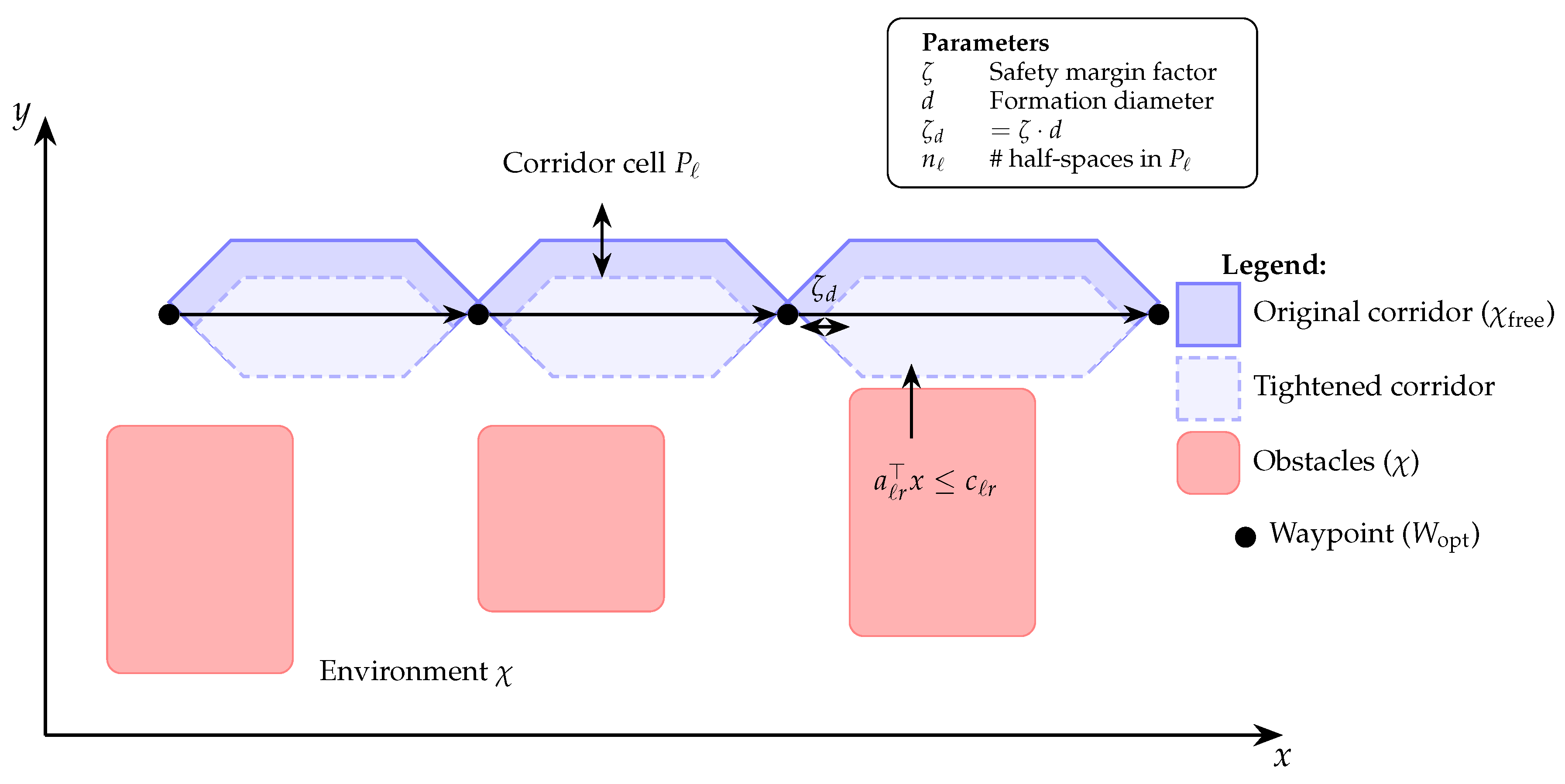
Figure 1.
Schematic of the safe flight corridor (SFC). The original corridor (solid blue) consists of convex polyhedra connecting optimized waypoints. Each supporting half-space is shifted inward by to obtain the tightened corridor (dashed blue), ensuring collision-free motion for a formation of diameter d.
3.2. Trajectory and Formation Size Generation
Within replanning iteration k, the leader trajectory is represented by an M-segment n-th order Bézier curve
where are control points and are Bernstein polynomials. Using the convex-hull property, containment in the safe flight corridor can be enforced by requiring all control points in the corresponding polyhedron.
We choose the formation size as an optimization variable jointly with control points and polyhedron assignment binaries :
A smooth transition between and is generated by a high-order polynomial satisfying boundary derivative matching up to order 4.
Remark 2.
The trajectory smoothness term is chosen as the integral of the squared jerk, i.e., , for the following reasons. First, the jerk directly reflects the rate of change of acceleration and is closely related to the smoothness of thrust and attitude commands of quadrotor UAVs, making it more suitable than acceleration-based costs for execution on real platforms. Second, when the trajectory is parameterized by Bézier curves, the jerk remains a low order polynomial, which leads to a quadratic cost in the control points and enables efficient MIQP formulation. Finally, higher-order smoothness is enforced through explicit bounds on snap, guaranteeing continuity and compatibility with geometric tracking controllers. This choice provides a favorable trade-off between trajectory smoothness, tracking feasibility, and computational efficiency.
3.3. Distributed Time-Varying Formation Control under Switching Topologies
To enable followers to compute and its derivatives, the leader publishes a parameter vector , which contains the current segment Bézier control points and timing information and the current formation-size polynomial parameters. Given and time t, any agent can compute and analytically. Since replanning occurs at discrete instants, is piecewise constant with bounded jumps and bounded update frequency.
For each coordinate , define the scalar estimate and the leader signal . We propose the nonlinear agreement protocol with delays:
where
and the nonlinearity satisfies the strict dissipativity condition.
Assumption 3.
For each coordinate ℓ, , and for all , . Moreover, is locally Lipschitz and there exists a class- function such that for all r in the semi-global domain of interest.
Define the leader oscillation over the delay window:
(17)–(18) is a direct leader-following extension of the agreement model in [31]: each follower is driven toward a time-varying convex combination of delayed neighbor estimates and delayed leader signal. The core advantage is that its convergence can be established via max–min contraction arguments under Assumption 1, without requiring a common quadratic Lyapunov function for switching directed graphs.
Define the estimation error for coordinate ℓ: . Let
Note that due to the leader time-variation, the asymptotic tracking generally requires additional internal model structure. Here we establish agreement among followers, and practical tracking to the leader with a bound proportional to .
Theorem 1.
Suppose Assumptions 1, 3 and bounded delays (7) hold. Then for each coordinate ℓ:
- 1.
-
the follower disagreement width converges to a neighborhood of zero:for some class- function determined by and the joint leader reachability window . In particular, if is piecewise constant, then on each constant interval.
- 2.
-
each follower error satisfies the practical boundwhere is explicitly constructible via the window based contraction recursion as in [31].
Proof.
We prove the result for a single scalar coordinate of the leader parameter vector . The vector case follows by applying the same argument componentwise and taking the maximum bounds.
Define the follower envelope over the delay window
and the width . By Lemma 3, for all i and all t,
Applying Lemma 2 to each estimator implies that cannot exit the convex hull generated by , and the leader window. Hence is well-defined and uniformly bounded for all .
By Assumption 1, for any t there exists a time window whose union graph contains a directed spanning tree rooted at some follower r that receives leader information (i.e., on a subinterval of length at least ). Applying Lemma 4 on this subinterval shows that moves away from the envelope extremes by a margin proportional to , up to the leader window oscillation .
Along each directed edge of the spanning tree, Assumption 1 guarantees persistence for at least and a uniform weight lower bound . By Lemma 5, the contraction margin at the root propagates to each downstream node with at least a factor per edge. Since the depth of the spanning tree is at most , after the window every follower contracts toward the interior of the envelope.
Then there exist explicit constants
such that for all ,
Iterating this recursion proves that: (i) if is constant on , then strictly contracts and as ; and (ii) for time-varying , is ultimately bounded by .
The proof is complete. □
Each follower i reconstructs the leader reference and its derivatives from :
where and are analytic maps induced by Bézier/polynomial parameterization. Then the follower’s desired trajectory and derivatives are
Finally, each follower applies a geometric tracking controller using , , , etc.
Given the implemented reference and yaw with bounded derivatives up to order four, we adopt a standard geometric tracking controller on (e.g., [32]). Define the position/velocity errors
A commanded acceleration is chosen as
and the thrust is set to
The desired attitude is constructed from the commanded acceleration and yaw. Its corresponding reference angular velocity is defined by
where denotes the vee map from to .
The desired attitude is constructed such that aligns with and the yaw matches . Then the moment input is designed by a standard attitude error feedback controller
which guarantees exponential tracking of to for sufficiently smooth references. This yields the ISS-type bound in Lemma 7.
Assumption 4.
For each coordinate ℓ, the function is continuous, locally Lipschitz, , and there exists a constant such that
Remark 3.
Assumption 4 is a standard strong dissipativity/sector condition. It implies the sign condition for used in the switching agreement literature, while additionally providing a quantitative contraction rate that yields explicit recursion constants. A canonical choice is or .
Theorem 2.
Under Assumptions 1–3, and bounded delays (7), the closed-loop system consisting of the online planner (12)–(16), the nonlinear estimators (17)–(18), and the tracking controllers, satisfies:
- 1.
- all estimation signals are uniformly bounded for all .
- 2.
- the reconstructed references , are uniformly bounded and satisfy the practical tracking bounds implied by Theorem 1.
- 3.
-
the formation tracking error is ultimately bounded:where can be made arbitrarily small by increasing the estimator contraction gain.
Proof.
The proof proceeds by a cascade argument.
By Theorem 1, for each follower i the leader parameter estimation error satisfies
and exponentially on any interval, where and are two positive constants.
By Lemma 6, the reconstructed reference trajectory and its derivatives satisfy
for some constants . Hence, the reference mismatch is uniformly bounded and vanishes whenever .
By Lemma 7, the single-UAV tracking error satisfies
where and are two positive constants.
Taking the limit superior and combining with (25) yields
for some constant .
Substituting the estimator bound from (24) completes the proof. In particular, on any replanning interval where is constant, the formation tracking error converges exponentially to zero. □
4. Lemmas and Main Proofs
The following presents several important lemmas and their proofs required for the proofs of Theorems 1–2.
Lemma 1.
Under Assumptions 3 and bounded delays (7), for each ℓ, the follower envelope satisfies for almost all t
where and are appropriate max/min convex-combination bounds induced by (18).
Proof.
Pick an index . Using the Dini derivative of a pointwise maximum and the dynamics (17),
By Assumption 3, is sign-definite and drives toward . Since is a convex combination of delayed neighbor estimates and leader signal, it lies between the delayed envelopes. This yields an inequality in terms of and the delayed envelopes. The bound for is analogous by choosing . □
Lemma 2.
Consider the scalar system
where is measurable and satisfies for all t. Assume (23) holds with gain for φ. Then for almost all t,
and
where . In particular, if and are constant on an interval , then for all ,
Proof.
Lemma 3.
For all and each follower i,
Moreover, if on a time subinterval, then is astrictconvex combination in the sense that it lies at least a fraction toward the leader window interval.
Proof.
Lemma 4.
Under Assumption 4 and bounded delays. Fix an interval with such that for some follower r, for all . Then on I,
where ⊕ denotes Minkowski sum of intervals, , and the contraction margin
In particular, if is constant on I then and moves at least away from the follower envelope extremes.
Proof.
Let and . Consider the upper deviation on I. By Lemma 3, . Hence . Applying Lemma 2 with yields an exponential decay of up to the variation of . A symmetric argument holds for the lower deviation using . Combining both bounds and noting that the leader-window variation within I is captured by gives (36). The explicit margin (37) follows by integrating the exponential contraction over and using that strict leader weight pulls toward the leader interval by a fraction . □
Lemma 5.
Under Assumption 4, consider an interval with during which a directed edge is continuously active and has weight lower bounded as for all . If at time the source node satisfies
for some , then the target node satisfies at
where accounts for leader variation entering through other neighbors/leader.
Proof.
On the set I, includes the term with weight at least . Since delayed stays in over the relevant delay window, and all other terms lie in (by definition of envelopes), we obtain bounds:
up to leader variation . Then Lemma 2 yields that is attracted to the tightened interval with exponential rate k, producing the margin after time . □
Lemma 6
(Lipschitz reference reconstruction). Let encode the active Bézier segment control points and timing information, and the formation-size polynomial parameters, so that and for . Assume the planner ensures boundedness of and excludes singular timing (i.e., segment durations are bounded away from 0). Then for each compact time interval between replannings and for each , there exist constants such that
Proof.
For Bézier curves and polynomials, and are smooth functions of the parameters on any set where segment durations are bounded away from zero. Thus their Jacobians are bounded on the compact parameter set induced by the planner bounds, implying local Lipschitz continuity with constants . □
Lemma 7.
Consider follower UAV i with dynamics (1) controlled by a geometric tracking controller that achieves exponential tracking for a reference trajectory. Let the controller be driven by animplementedreference and its derivatives up to order 4, while the ideal formation reference is . Define the position tracking error . Then there exist constants and such that
Proof.
For flatness-based geometric controllers, the closed-loop tracking error dynamics can be written in a cascade form with an exponentially stable linear part plus bounded higher-order terms that are dominated by the reference mismatch. Under bounded reference derivatives and standard gain conditions, one obtains an exponential Lyapunov function satisfying . Gronwall’s inequality yields (39). □
5. Simulation Results
In this section, we employ a numerical example to verify the effectiveness of the proposed algorithm.
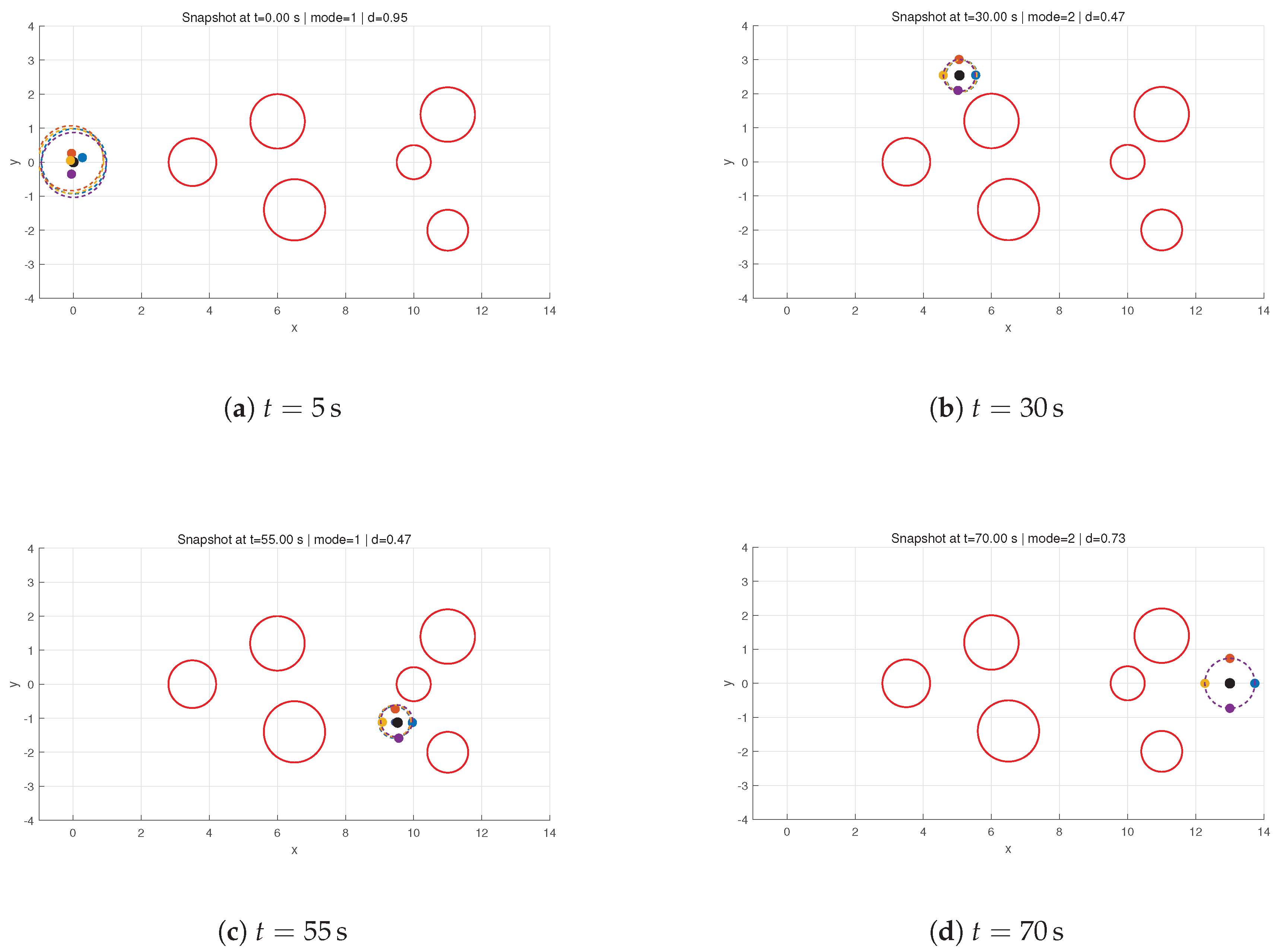
We consider a planar multi-UAV formation navigation task in an obstacle environment. The team consists of 5 UAVs, including one leader indexed by 0 and followers indexed by . The leader starts from and aims to reach the goal . The environment contains six static circular obstacles, specified by their centers and radius:
where each triple denotes .
Followers are required to maintain a time-varying circular formation around the leader reference trajectory . Let be the desired angular offsets equally spaced on a circle. Define . The ideal formation reference for follower i is
where is the time-varying formation radius.
Communication among followers is described by a directed switching graph with three modes. We use the adjacency matrix , where indicates a directed edge (i.e., follower j receives information from follower i) under mode m. The three modes are:
The topology switches periodically every . In addition, the leader information is directly available to exactly one follower per mode, encoded by :
Communication delays are time-varying but bounded by .
This subsection lists the simulation parameters and briefly verifies that the theoretical assumptions are satisfied. The simulation runs with sampling time over . The leader replans every . The input of UAVs are speed with saturation for the leader and for followers. The leader tracks the planned reference point by a proportional law
with . Followers track their formation references using
with , where is a light obstacle repulsion term for safety.
The leader generates a waypoint list (with and ) and constructs a safe flight corridor as a sequence of convex polyhedra
In implementation, each is initialized as an axis-aligned corridor box inflated by and then tightened by obstacle separating half-planes. The leader trajectory over each corridor segment is parameterized by a quintic Bézier curve (). The control points are obtained by solving a quadratic program that minimizes a discrete proxy of the integrated squared jerk (third differences of control points), with weight .
The nominal formation radius is and the minimum radius is . The corridor tightening uses the safety factor , so that the corridor constraints are reduced by approximately at each replanning iteration (consistent with the formation footprint). The planned radius is smoothed into using a first-order filter with time constant .
Each follower maintains an estimate of the leader reference point using the nonlinear agreement protocol with delays:
where is a convex combination of delayed neighbor estimates and (when available) the leader reference:
with normalized weights and defined as in (6). Delays satisfy and are simulated by random discrete delays up to steps.
The directed switching graphs (41) together with leader access vectors (42) ensure that within each switching window the leader information can reach all followers through directed paths, satisfying the joint leader reachability condition. The delay bound is enforced by construction. The nonlinearity satisfies and for all , fulfilling the strict dissipativity requirement. Therefore, the Assumptions 1–4 of the theoretical analysis are satisfied in simulation.
The leader starts at . Each follower starts near the leader with small random perturbations around the desired circular formation positions. The initial estimator states are also perturbed, resulting in nonzero initial estimation errors. The simulation results are shown as in Figure 2, Figure 3, Figure 4, Figure 5, Figure 6 and Figure 7. Figure 2 shows the trajectories of the leader and followers. The leader successfully navigates through the cluttered environment and reaches the goal, while followers maintain the desired circular formation. As the team approaches narrow passages, the formation radius decreases, enabling the entire formation to remain within the safe corridor, and then increases again in open regions. Figure 3 compares the planned leader reference trajectory and the executed leader trajectory . The executed trajectory closely tracks the planned reference, demonstrating that the planned trajectory is sufficiently smooth for tracking. Figure 4 plots the time evolution of the formation radius , showing adaptive shrink behavior consistent with obstacle proximity. Figure 5 reports the distributed estimator errors for all followers. Figure 6 illustrates the mode switching process of the topology, while Figure 7 shows a screenshot of the animation depicting the collective motion of the moving bodies in formation. Despite switching directed communication topologies and bounded delays, the estimator errors remain bounded and converge to small neighborhoods of zero, which corroborates the practical agreement guarantee.
The simulation results validate the proposed framework in a cluttered environment: (i) online planning generates smooth safe trajectories; (ii) adaptive formation sizing enables obstacle avoidance for the entire team; and (iii) the distributed nonlinear estimator achieves robust leader-reference tracking under directed switching graphs with delays, leading to successful distributed formation control.
6. Conclusions
This paper presented a distributed formation planning and control framework for multi-UAV systems operating under directed switching communication topologies and environmental constraints. By integrating SFC-based trajectory planning with adaptive formation sizing, the proposed method enables the entire formation to safely navigate obstacle-rich environments. A nonlinear agreement protocol was introduced to handle delayed and intermittent leader information, and rigorous analysis established practical tracking and agreement guarantees under switching graphs. Simulation results validated the theoretical findings and demonstrated robust performance in challenging scenarios. Future work will focus on extending the framework to fully three-dimensional environments, incorporating more complex vehicle dynamics, and investigating experimental validation on real UAV platforms.
Author Contributions
Conceptualization, Z.Y. and J.Z; methodology, Z.Y. and J.Z.; software, Z.Y.; validation J.Z.; formal analysis, Z.Y. and J.Z.; investigation, Z.Y.; writing—original draft preparation, Z.Y. and J.Z.; writing—review and editing, Z.Y. and J.Z.; visualization, Z.Y.; supervision, Z.Y. and J.Z.; project administration, Z.Y. and J.Z. All authors have read and agreed to the published version of the manuscript.
Funding
TThis work was supported in part by the Natural Science Foundation of China under Grant 62403423, and the Natural Science Foundation of Zhejiang Province under Grant LMS25F030003.
Institutional Review Board Statement
Not applicable.
Informed Consent Statement
Not applicable.
Data Availability Statement
Not applicable.
Conflicts of Interest
The authors declare no conflicts of interest.
References
- Chowdhury, M.M.U.; Maeng, S.J.; Bulut, E.; Güvenç, ˘I. 3-D Trajectory Optimization in UAV-Assisted Cellular Networks Considering Antenna Radiation Pattern and Backhaul Constraint. IEEE Transactions on Aerospace and Electronic Systems 2020, 56, 3735–3750. [CrossRef]
- Bao, T.; Wang, H.; Wang, W.J.; Yang, H.C.; Hasna, M.O. Secrecy Outage Performance Analysis of UAV-Assisted Relay Communication Systems With Multiple Aerial and Ground Eavesdroppers. IEEE Transactions on Aerospace and Electronic Systems 2022, 58, 2592–2600. [Google Scholar]
- Hung, H.A.; Hsu, H.H.; Cheng, T.H. Optimal Sensing for Tracking Task by Heterogeneous Multi-UAV Systems. IEEE Transactions on Control Systems Technology 2024, 32, 282–289. [Google Scholar] [CrossRef]
- Gong, X.; Gui, J.; Chen, Y.; Yang, X.; Yu, W.; Huang, T. Resilient Human-in-the-Loop Formation-Tracking of Multi-UAV Systems Against Byzantine Attacks. IEEE Transactions on Automation Science and Engineering 2025, 22, 3797–3809. [Google Scholar]
- Hai, X.; Tan, L.; Feng, Q.; Duan, H.; Wen, C. Replanning-Oriented Framework for Efficient Real-Time Decision-Making in Multi-UAV Systems. IEEE Transactions on Industrial Informatics 2025, 21, 5127–5137. [Google Scholar]
- Ma, J.; Chen, X.; Wen, G.; Wang, J.; Zhao, F.; Qiu, J. Dynamic Memory Event-Triggered Lag Consensus of Multi-UAV Systems With Hybrid Attacks Over Stochastic Switching Topology. IEEE Transactions on Automation Science and Engineering 2025, 22, 16999–17009. [Google Scholar]
- Savkin, A.V.; Huang, H. Multi-UAV Navigation for Optimized Video Surveillance of Ground Vehicles on Uneven Terrains. IEEE Transactions on Intelligent Transportation Systems 2023, 24, 10238–10242. [Google Scholar] [CrossRef]
- Cao, X.; Liu, L. A Multi-Timescale Method for State of Charge Estimation for Lithium-Ion Batteries in Electric UAVs Based on Battery Model and Data-Driven Fusion. Drones 2025, 9, 247. [Google Scholar]
- El-Malek, A.H.A.; Aboulhassan, M.A.; Salhab, A.M.; Zummo, S.A. Performance Analysis and Optimization of UAV-Assisted Networks: Single UAV With Multiple Antennas Versus Multiple UAVs With Single Antenna. IEEE Systems Journal 2023, 17, 3468–3479. [Google Scholar] [CrossRef]
- Li, Y. Cooperative Elliptic Positioning Through Single UAV During GNSS Outages. IEEE Transactions on Wireless Communications 2024, 23, 12749–12764. [Google Scholar] [CrossRef]
- Dong, X.; Yu, B.; Shi, Z.; Zhong, Y. Time-Varying Formation Control for Unmanned Aerial Vehicles: Theories and Applications. IEEE Transactions on Control Systems Technology 2015, 23, 340–348. [Google Scholar]
- Ranjan, P.K.; Sinha, A.; Cao, Y.; Casbeer, D.; Weintraub, I. Relational Maneuvering of Leader-Follower Unmanned Aerial Vehicles for Flexible Formation. IEEE Transactions on Cybernetics 2024, 54, 5598–5609. [Google Scholar] [CrossRef]
- Yang, Y.; Sun, L.; Fu, Y.; Feng, W.; Xu, K. Three-Dimensional UAV Trajectory Planning Based on Improved Sparrow Search Algorithm. Symmetry 2025, 17, 2071. [Google Scholar] [CrossRef]
- Seyyedabbasi, A. Multi-Strategy Variable Secretary Bird Optimization Algorithm (MSVSBOA) for Global Optimization and UAV 3D Path Planning. Symmetry 2026, 18, 273. [Google Scholar] [CrossRef]
- Jin, Z.; Bai, L.; Wang, Z.; Zhang, P. Self-Triggered Distributed Formation Control of Fixed-Wing Unmanned Aerial Vehicles Subject to Velocity and Overload Constraints. IEEE Transactions on Automation Science and Engineering 2024, 21, 4082–4093. [Google Scholar]
- Jin, Z.; Li, H.; Qin, Z.; Wang, Z. Gradient-Free Cooperative Source-Seeking of Quadrotor Under Disturbances and Communication Constraints. IEEE Transactions on Industrial Electronics 2025, 72, 1969–1979. [Google Scholar]
- Dong, X.; Zhou, Y.; Ren, Z.; Zhong, Y. Time-Varying Formation Tracking for Second-Order Multi-Agent Systems Subjected to Switching Topologies With Application to Quadrotor Formation Flying. IEEE Transactions on Industrial Electronics 2017, 64, 5014–5024. [Google Scholar]
- Zou, Y.; Zhou, Z.; Dong, X.; Meng, Z. Distributed Formation Control for Multiple Vertical Takeoff and Landing UAVs With Switching Topologies. IEEE/ASME Transactions on Mechatronics 2018, 23, 1750–1761. [Google Scholar] [CrossRef]
- Shi, S.; Wu, S.; Wei, B. Neural-Network-Based Event-Triggered Formation Tracking for Nonlinear Multi-UAV Systems With Switching Topologies Under DoS Attacks. IEEE Transactions on Automation Science and Engineering 2025, 22, 11656–11667. [Google Scholar]
- Dong, Z.; Shi, S.; Zhen, Z. Asynchronously Integral Event-Triggered Formation Tracking in UAV Swarm Systems Featuring Switching Directed Topologies. IEEE Transactions on Control of Network Systems 2025, 12, 1251–1263. [Google Scholar] [CrossRef]
- Proskurnikov, A.V.; Calafiore, G.C. Delay Robustness of Consensus Algorithms: Continuous-Time Theory. IEEE Transactions on Automatic Control 2023, 68, 5301–5316. [Google Scholar]
- Wu, H.; Meng, D. Synchronizability-Based Distributed Learning Control for Multi-Agent Systems. IEEE Transactions on Circuits and Systems II: Express Briefs 2024, 71, 2109–2113. [Google Scholar] [CrossRef]
- Li, F.; Wang, C.; Mikulski, D.; Wagner, J.R.; Wang, Y. Unmanned Ground Vehicle Platooning Under Cyber Attacks: A Human-Robot Interaction Framework. IEEE Transactions on Intelligent Transportation Systems 2022, 23, 18113–18128. [Google Scholar] [CrossRef]
- Schäfer, L.; Manzinger, S.; Althoff, M. Computation of Solution Spaces for Optimization-Based Trajectory Planning. IEEE Transactions on Intelligent Vehicles 2023, 8, 216–231. [Google Scholar] [CrossRef]
- Guo, Z.; Wang, Y.; Yu, H.; Xi, J. Fast Optimization-Based Trajectory Planning With Cumulative Key Constraints for Automated Parking in Unstructured Environments. IEEE Transactions on Vehicular Technology 2025, 74, 11820–11831. [Google Scholar] [CrossRef]
- Olfati-Saber, R.; Murray, R.M. Consensus Problems in Networks of Agents With Switching Topology and Time-Delays. IEEE Transactions on Automatic Control 2004, 49, 1520–1533. [Google Scholar] [CrossRef]
- Lin, Z.; Francis, B.; Maggiore, M. State Agreement for Continuous-Time Coupled Nonlinear Systems. SIAM Journal on Control and Optimization 2007, 46, 288–307. [Google Scholar] [CrossRef]
- Shi, G.; Hong, Y. Global Target Aggregation and State Agreement of Nonlinear Multi-Agent Systems With Switching Topologies. Automatica 2009, 45, 1165–1175. [Google Scholar] [CrossRef]
- Cong, X.; Zi, L.; Du, D.Z. DTNB: A Blockchain Transaction Framework With Discrete Token Negotiation for the Delay Tolerant Network. IEEE Transactions on Network Science and Engineering 2021, 8, 1584–1599. [Google Scholar] [CrossRef]
- Liu, T.; Qin, Z.; Hong, Y.; Jiang, Z.P. Distributed Optimization of Nonlinear Multiagent Systems: A Small-Gain Approach. IEEE Transactions on Automatic Control 2022, 67, 676–691. [Google Scholar] [CrossRef]
- Wang, Z.X.; Jin, Z.H.; Li, H. Semi-global asymptotic state agreement of nonlinear multi-agent systems with communication delays under directed switching topologies. Nonlinear Analysis: Hybrid Systems 2024, 52. [Google Scholar]
Figure 2.
The trajectories of the leader and followers.
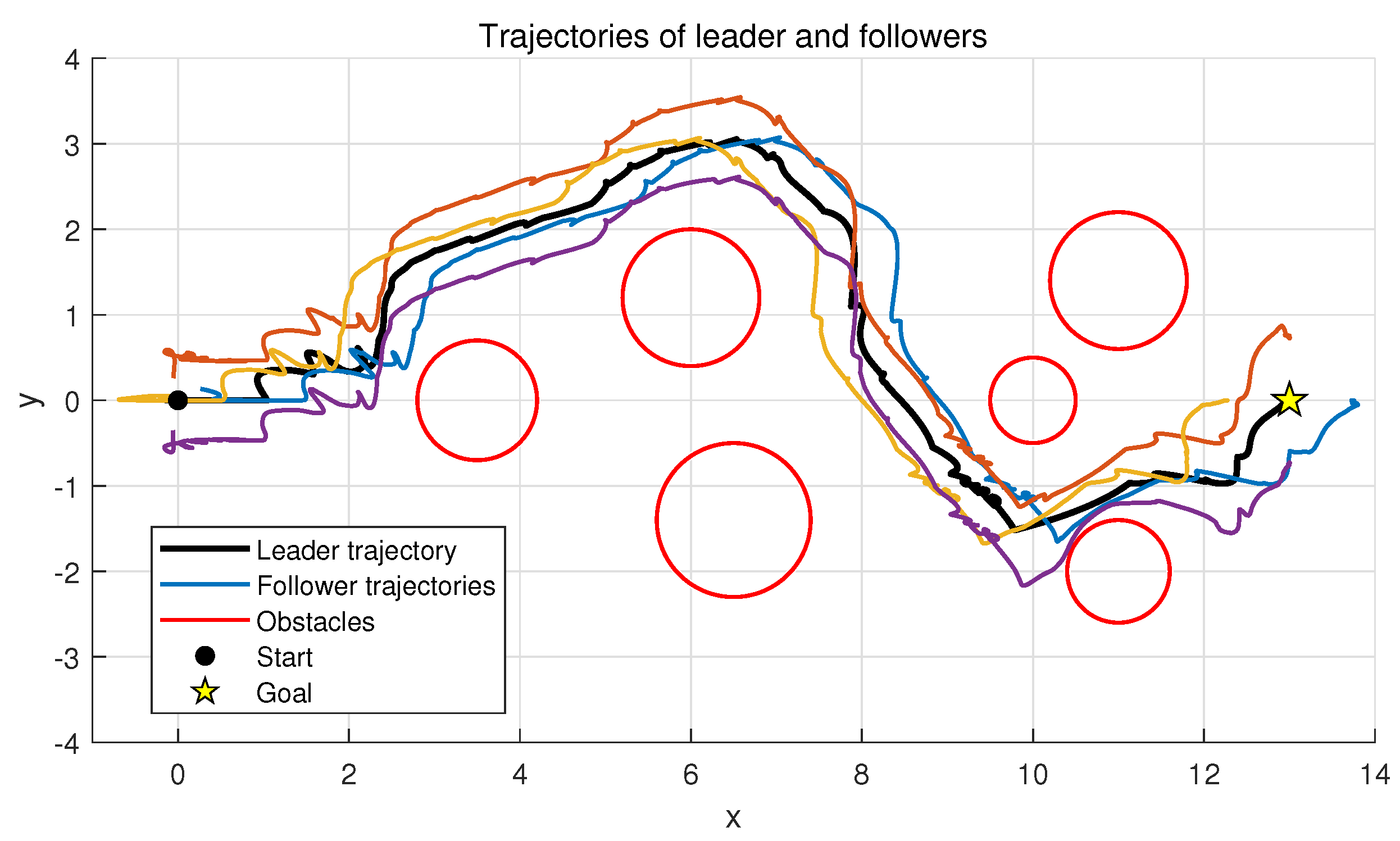
Figure 3.
The planned leader reference trajectory and the executed leader trajectory .
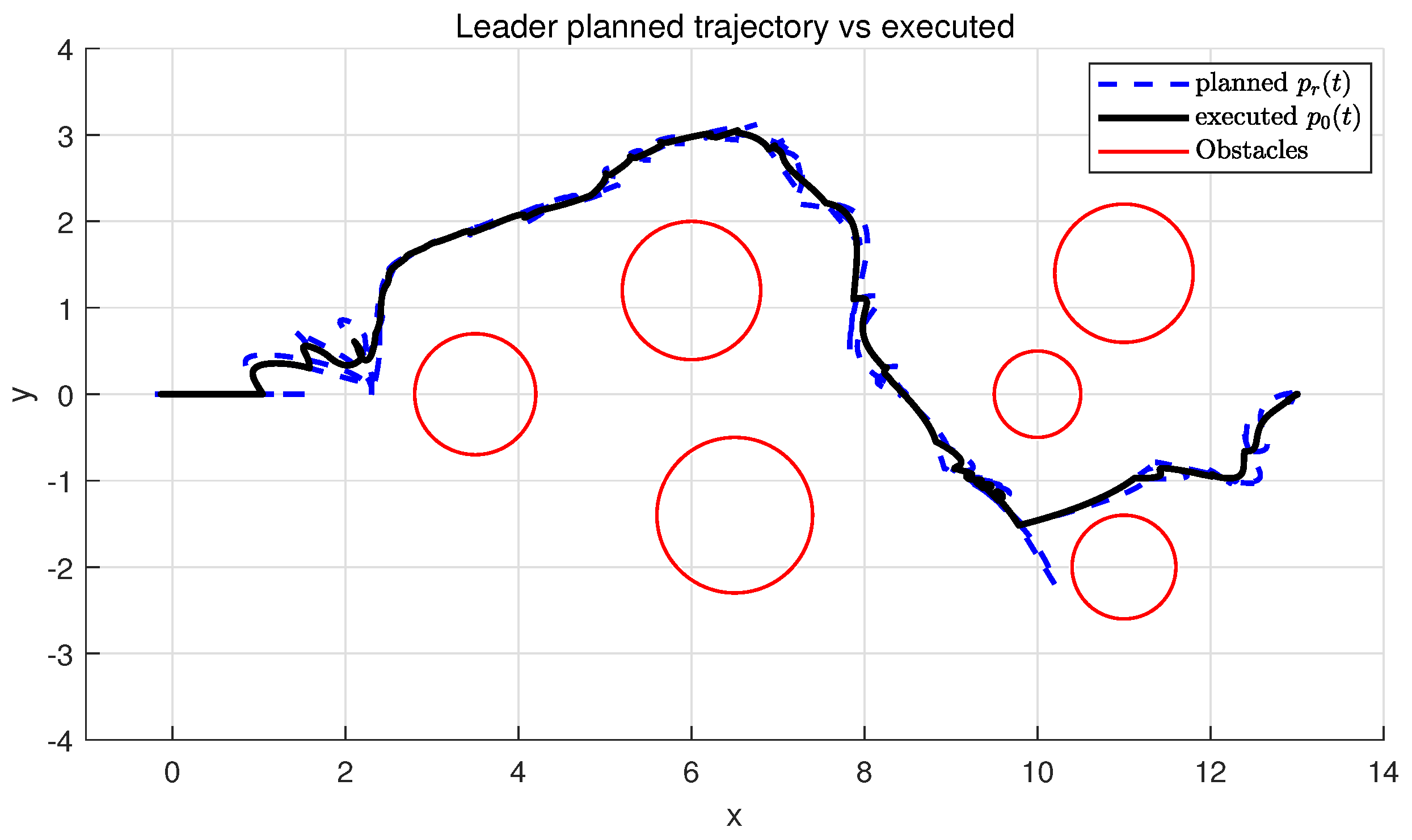
Figure 4.
Time evolution of the formation radius .
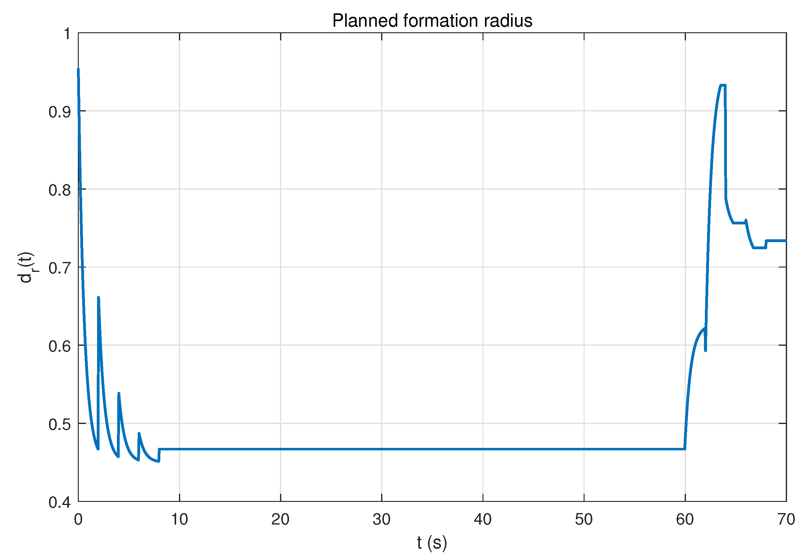
Figure 5.
the distributed estimator errors for all followers.
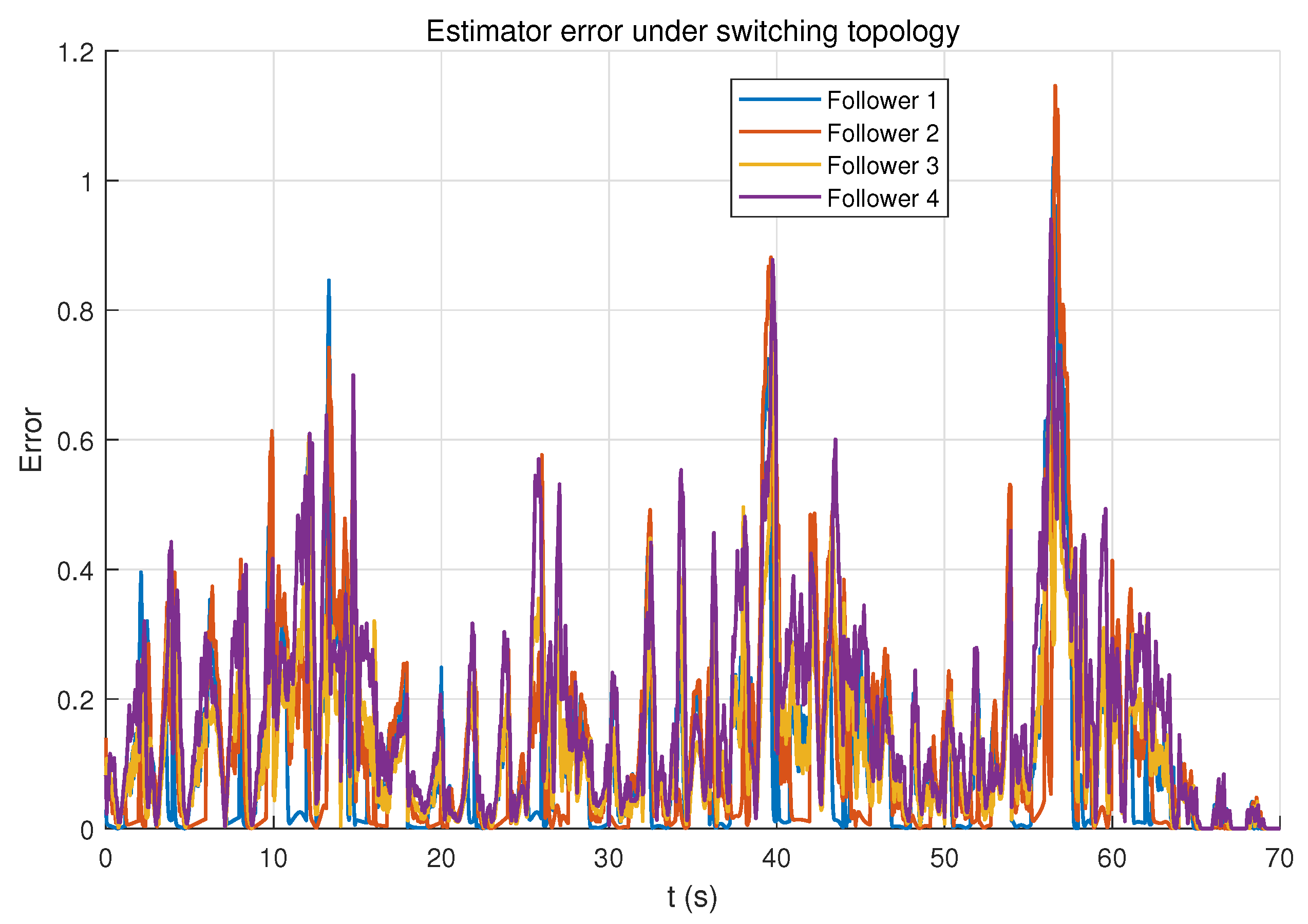
Figure 6.
The mode of switching topology.
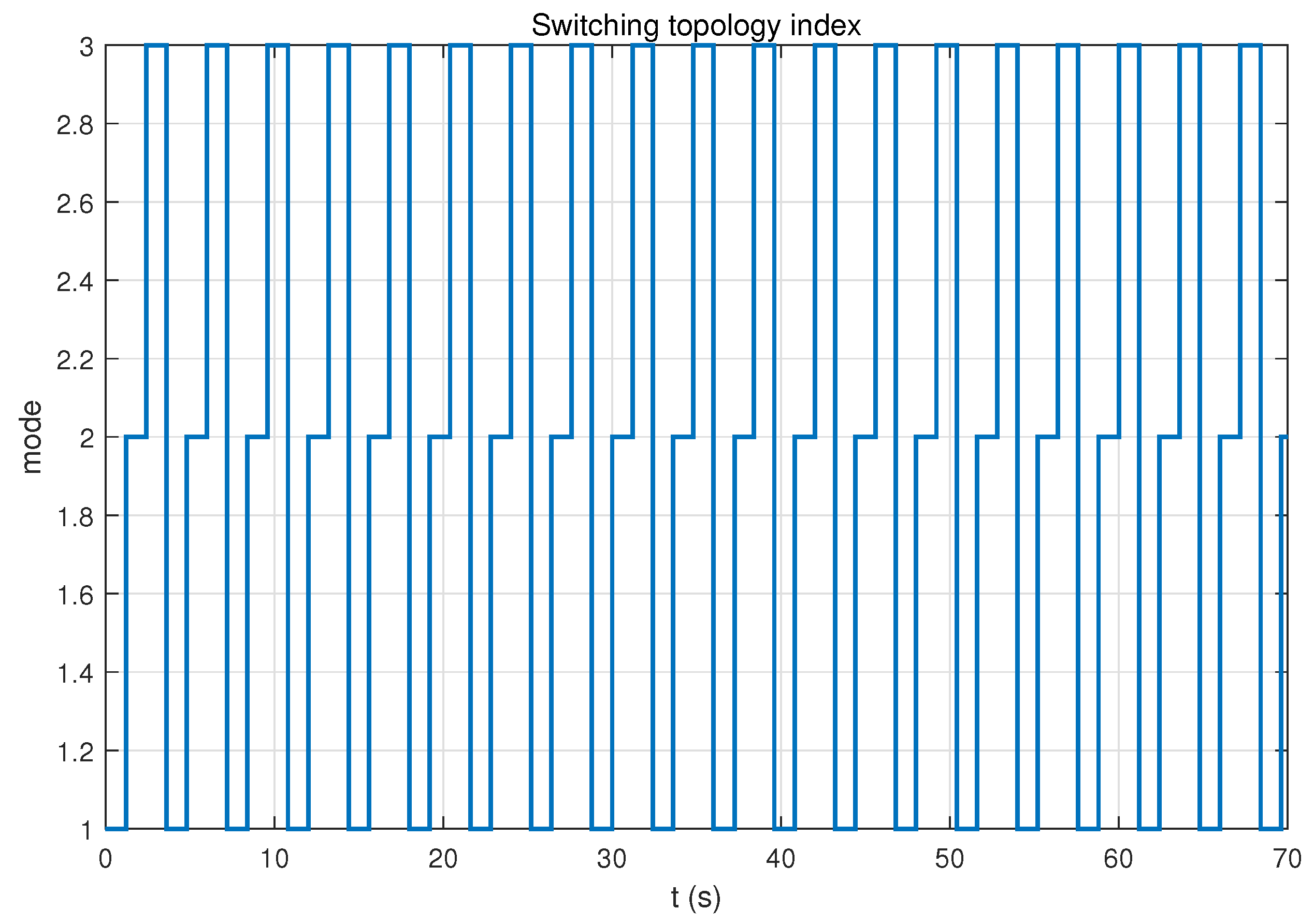
Figure 7.
Four snapshots (2×2) of the formation navigation under switching topologies.
Disclaimer/Publisher’s Note: The statements, opinions and data contained in all publications are solely those of the individual author(s) and contributor(s) and not of MDPI and/or the editor(s). MDPI and/or the editor(s) disclaim responsibility for any injury to people or property resulting from any ideas, methods, instructions or products referred to in the content. |
© 2026 by the authors. Licensee MDPI, Basel, Switzerland. This article is an open access article distributed under the terms and conditions of the Creative Commons Attribution (CC BY) license (http://creativecommons.org/licenses/by/4.0/).
Copyright: This open access article is published under a Creative Commons CC BY 4.0 license, which permit the free download, distribution, and reuse, provided that the author and preprint are cited in any reuse.


