Submitted:
13 February 2026
Posted:
14 February 2026
You are already at the latest version
Abstract
Vibrations of thin sheet-metal parts during robotic manipulation on a production line create a number of serious challenges for production process planning. Modeling the behavior of an elastic plate or shell as a function of the robot manipulator trajectory is typically performed using the finite element method (FEM) and requires significant computational effort. The time factor remains a key limitation for integrating operations involving flexible parts into the virtual commissioning process. In this work, a methodology is proposed that enables accurate real-time reproduction of the behavior of an elastic part during linear robotic manipulation. The approach is based on modeling the response of an elastic part to a prescribed base excitation using the FEM and on the development of a reduced model compliant with the FMI/FMU standard. This reduced model computes, in real time, the convolution of the precomputed base response with the acceleration profile corresponding to the robot TCP trajectory. This makes it possible to determine the total cycle duration, which consists of the part transfer time and the time required for vibration decay at the end of the trajectory down to an acceptable threshold, as well as to perform collision checking while accounting for the deformation of the flexible part. As a result, operations involving elastic parts can be integrated into the virtual commissioning process.
Keywords:
virtual commissioning
; finite element method
; flexible parts
; robotic manipulations
; FMI/FMU modeling
1. Introduction
Virtual commissioning of robotic production lines is widely applied across various industrial sectors. A digital model makes it possible to design and tune a complex production system consisting of equipment, conveyors, robots, sensors, and controllers prior to its physical assembly. However, current virtual commissioning systems do not yet support manipulations involving flexible parts. In virtual environments, robots successfully perform operations with rigid bodies, for which the positions of points can be easily computed at any moment in time. The review paper [26] addresses various issues arising in the planning of manipulations involving deformable objects such as ropes, cloth, paper, and sheet metal.
When manipulating thin sheet-metal parts, two types of difficulties arise. The first is that during accelerated motion the part begins to vibrate and its shape changes, which complicates collision detection. The second difficulty is even more significant: the cycle time becomes uncertain since, in addition to the transportation time, it now includes the time required for the decay of residual vibrations at the end of the trajectory. In many production operations, the transition to the fixation stage (e.g., welding or adhesive bonding) is only possible after the vibration amplitude in the fixation area has decreased to an acceptable level. Thus, for example, a welding robot must wait for an additional period of time, the duration of which strongly depends on the part geometry, material properties, the placement of vacuum suction cups, and the motion trajectory.
To address vibration-related issues in the automotive industry, specialized vacuum grippers are used that hold the flexible part over its entire surface and practically eliminate vibrations. This solution makes both real and virtual operations with flexible parts equivalent to manipulations with rigid bodies: the geometry does not change during motion, and the cycle time is equal to the transportation time. However, this approach has several drawbacks. Such vacuum grippers are expensive, with a cost comparable to that of the robot itself; they are bulky, which complicates workspace organization; and they are heavy, requiring robots with higher payload capacity and, consequently, higher cost. In addition, such grippers must be manually adapted to the geometry of each specific part. In [2], the problem of optimizing a stamping line is also described, where an excessively large gripper requires more time to be withdrawn from under the press after positioning the metal blank, leading to delays in the stamping process.
We propose an alternative solution (Figure 1) based on the use of a simple and universal gripper, which is cheaper, lighter, more compact, and easier to adapt to a specific part. However, the effective application of such a gripper requires solving several important tasks:
- the ability to rapidly compute the behavior of a flexible part as a function of the robot trajectory;
- the ability to accurately estimate the decay time of residual vibrations at the end of the trajectory.
Based on this, it may be possible to determine an optimal robot trajectory that minimizes the total cycle time, i.e., the sum of the time required to move the part and the decay time of residual vibrations at the end of the trajectory. In [2], we present a methodology that outlines the steps for constructing an optimal trajectory. The key difficulty in this process is the need to perform FEM simulations of the flexible part’s behavior during the production cycle.
In order for FEM simulation results for thin sheet-metal parts to be realistic, a mesh with tens or even hundreds of thousands of nodes is required, which leads to transient analyses lasting tens of minutes. Numerical studies indicate that even when shell elements are employed for large components with complex geometry, meshes consisting of only 1–2 thousand nodes may lead to errors in the predicted natural frequencies in the range of 20% to 100%. However, for virtual commissioning of operations with flexible parts—and even more so for the search for an optimal trajectory, where each iteration of the optimization algorithm requires a new FEM simulation—it is necessary for such calculations to be performed in real time.
It should be noted that in the NVIDIA Omniverse environment, the behavior of flexible bodies is simulated in real time using the Physics 5.0 solver, based on the methodology described in [2]. This physical model has proven effective in the gaming industry and medical simulations; however, it does not accurately represent reality for elastic bodies such as thin metal parts. Thus, the search for methods that significantly accelerate FEA (finite element analysis) remains highly relevant, and this issue has been addressed by many authors.
First, we note the works [2,2], which investigate the optimization of sheet-metal operations. Both studies use the same approach: in the first stage, a large number of FEM simulations are used to construct surrogate models for the maximum displacement of points on the metal sheet from their initial positions and the maximum von Mises stress as a function of the TCP acceleration vector of the robot. In the second stage, an optimal robot trajectory is determined, minimizing the cycle time while considering several constraints, such as obstacle avoidance, acceleration limits achievable by the robot, and the condition that stresses in the metal must not exceed the plastic deformation threshold.
However, these studies considered only simple geometries, such as a rectangular plate. The part’s response to acceleration at each time step did not take into account that after the previous step, the part is already in a deformed and stressed state. Quadratic regression was used to construct the surrogate model, which allows approximating function values but does not correspond to the physical meaning of the underlying processes.
In the review article [2], various methods for constructing surrogate models are presented, which have proven effective for computations based on the finite element method. Methods such as Response Surfaces and Linear Regression, Kriging, Multilayer Perceptron (MLP), Boosted Trees, and Random Forests allow the construction of surrogate models, for example, for the maximum displacement of points of a part, the maximum von Mises equivalent stress, and the decay time of residual vibrations as a function of the robot trajectory with a flexible part. At the same time, building such models requires a large amount of training data, i.e., thousands of FEM simulations, and the accuracy of these models significantly decreases with high-dimensional input parameters. Some of these methods are already implemented as standard in the ANSYS Workbench software package, and the ANSYS documentation provides examples showing how the choice of surrogate modeling method can substantially influence optimization results in structural mechanics problems.
In [2], a comparative analysis of various machine learning (ML) and deep learning (DL) methods for constructing surrogate models to accelerate FEM simulations in structural mechanics tasks was conducted. Test cases included: static structural analysis of a perforated plate under tension, beam bending, and compression of a block with holes. For each method, the authors evaluated the model accuracy (using the coefficient of determination , as the metric) and inference time. In all considered problems, the best-performing methods achieved an close to 0.99 and demonstrated up to a hundredfold acceleration compared to FEM simulation. It is important to note that the analysis was performed on bodies of simple geometry with dimensions around 10 cm × 20 cm. Even in this case, for a relatively simple neural network architecture, the inference time was 70 milliseconds, whereas the standard FEM simulation took 9 seconds, which is still far from real-time. For larger parts with complex geometries, the inference time may increase to several seconds or more.
In [2], a comprehensive review of neural network–based surrogate models (MLP, CNN, GNN, RNN, LSTM, PINNs) for static structural analysis was conducted. The study demonstrated that these methods have significant potential to accelerate FEM simulations by a factor of 50 to 1000, depending on the problem. However, several major challenges were highlighted: the need for a large and high-quality training dataset, relatively limited generalization capabilities for many types of neural networks (changes in geometry, boundary conditions, material, and load beyond the training dataset), and the difficulty of implementing real-time computations for complex structures. Among neural network approaches, Physics-Informed Neural Networks (PINNs) stand out as they do not require a large training set and can serve as an alternative to traditional FEM solvers.
Recent work [9] is one of the few studies that specifically considers the construction of a surrogate model for transient analysis. It presents a neural network architecture that predicts the displacements of mesh nodes at each time step. The algorithm accounts for and corrects errors accumulated due to the large number of temporal iterations. The task consists of predicting the dynamic response of a metal plate to a force applied to its surface. The simulation lasts 1 second with a time step of 5 milliseconds (a total of 200 time steps). The mesh contains 81 nodes and 64 elements for the 2D mesh, and 243 nodes and 128 elements for the 3D mesh. To build the training dataset, 450 FEM simulations were performed for 2D and 2256 FEM simulations for 3D. It is important to note that the inference time for 2D was 0.2 s on a GPU and 2.35 s on a CPU, and for 3D 0.23 s on a GPU and 15.3 s on a CPU, which is still far from real-time computation.
Separately, Physics-Informed Neural Networks (PINNs) should be highlighted, as they effectively serve as an alternative FEM solver for partial differential equation problems. In [10], the potential of PINNs for static analysis of thin shells under gravity or applied loads is explored. It is noted that PINNs represent a promising alternative to the classical finite element method. This approach allows directly solving the boundary value problem for the differential equation describing shell behavior under load, thus avoiding several FEM limitations, such as over-stiffness and locking effects. Training PINNs does not require a training dataset as in other models. At the same time, the authors note that PINNs are currently not competitive with traditional FEM solvers in terms of computational efficiency.
In [11], PINNs are applied to construct a sequence of input signals that suppress residual vibrations (Input Shaping). The approach is demonstrated on a moving cart with a flexible rod attached, showing high effectiveness in systems with a large (practically infinite) number of modes. This method is potentially applicable, with varying degrees of complexity, to flexible beams, thin plates, and shells. In [12], an analytical approach is proposed for generating an input signal to suppress residual vibrations of a vertical thin rod mounted on a horizontally moving platform.
One of the promising approaches for significantly accelerating dynamic simulations is based on Graph Neural Networks (GNN), as described in [13]. The authors demonstrate a 100-fold acceleration compared to FEM simulation when predicting the dynamic behavior of cloth, flexible plates, and examples from hydro- and aerodynamics. This approach shows excellent performance for strongly nonlinear deformations and interacting bodies, providing high prediction accuracy and good generalization capability. However, it should be noted that in the case of the deformable plate, the mesh contained only 1271 nodes, so it is unclear whether this approach can achieve real-time computation for meshes with 10–100 times more nodes.
In [14], the forging process of a metal part (yoke) is modeled using a GNN. Process parameters (temperature, friction) and the initial FEM mesh, converted into a graph where nodes contain local features averaged over neighboring elements, are used as inputs. The model is trained to predict the final wear field on the surface of the dies. The authors claim to have reduced FEM simulation time from 110 minutes to 0.5 seconds. The meshes for the upper and lower dies contained 9215 and 6617 nodes, respectively, but the training dataset of only 30 simulations appears insufficiently representative.
In [15], a surrogate model based on GNN was constructed to compute von Mises stress in a thin rectangular plate with a circular hole. The plate was fixed on one side, while the opposite side was subjected to displacement. The training dataset included 500 FEM simulations with varying geometric parameters: plate dimensions, radius and position of the hole center, and different displacement values. The resulting neural network provided a significant speed-up compared to classical FEM. A similar GNN-based surrogate model for von Mises stress was constructed in [16], demonstrating good generalization ability under changes in geometry and boundary conditions.
Another important issue for virtual commissioning is the integration of the flexible part behavior model into the virtual production cycle. For example, [17] presents a concept for virtual commissioning of a deep drawing process for sheet metal. In the ISG Virtuos environment, an FMU model version 2.0 was used, which accepted inputs such as punch displacement, clamping force, etc., then called the ANSYS LS-DYNA solver with these parameters, and returned the displacements of several control points on the metal part after FEM simulation. To reduce FEM computation time, the number of mesh elements was drastically reduced, yet the simulation still required 7 seconds—far from real-time. This again highlights the need to develop accurate and computationally efficient models describing the dynamic behavior of flexible parts. Approaches to structural mechanics problems based on deep learning demonstrate significant acceleration of FEM simulations and have potential for further speed-up.
However, at present, they do not allow the construction of highly accurate surrogate models for real flexible parts. For example, an automotive fender requires more than 50,000 nodes when using 2D shell elements and about 400,000 nodes for 3D elements. Reducing the number of nodes by a factor of 10 introduces substantial errors in natural frequencies: in our studies, the first eigenfrequency increased from 10 Hz to 20 Hz. Therefore, achieving high accuracy requires constructing neural networks for meshes with a large number of nodes. This requires a significant amount of training data, while the main problem remains the inference time, which, for such a complex architecture, is far from real-time.
2. Problem Formulation
A thin sheet metal part, fixed at several points using vacuum suction cups, is moved by a robotic manipulator without rotation from a resting state at point A to point B along a certain trajectory (Figure 2). It is necessary to determine the positions of all points of the flexible part at each moment in time, as well as to calculate the decay time of the residual vibrations of the part to a specified threshold after stopping at point B.
This work considers an idealized scenario: gravity is neglected, air resistance is not taken into account, the fixation is assumed rigid instead of rubber vacuum suction cups, vibrations of the robot itself are neglected, and the damping coefficient is known.
2.1. Discretization of the Trajectory
Since, in a transient analysis without rotation, the inertial load is determined by the acceleration, by different motion trajectories we will understand different acceleration profiles along each coordinate axis. In the literature, for the sake of simplicity, a stepwise acceleration profile is often considered. This corresponds to a rigid motion profile, which excites a wide spectrum of the natural frequencies of the entire system and leads to increased wear of the equipment.
Therefore, we will employ a smooth acceleration profile with a finite and small jerk. Such a profile corresponds to robot trajectories that are used in practice. As the time discretization step, we choose , which is a reasonable value both for robot control and as a time step for the FEM solver in simulations of the dynamic behavior of a flexible part. Thus, the acceleration profile along each coordinate has the following form (Figure 3).
Such a profile can be specified as a set of numbers Naturally, this set must realize a motion over a prescribed distance L from point A to point B with zero initial and final velocities, and it must also satisfy the constraints on velocity, acceleration, and jerk given in the technical documentation of the robot manipulator. The duration of the accelerated motion of the part will be denoted by , which is an integer multiple of the chosen time step.
2.2. FEM Simulation Results
To analyze the dynamic behavior of a flexible part during its manipulation by a robot, the following information is required: the geometry of the part, defined by a CAD model; the physical properties of the material, specified by Young’s modulus, Poisson’s ratio, and the damping ratio ; the locations where the part is fixed; as well as the simulation duration which exceeds, with a safety margin, both the time required for transporting the part and the time needed for the residual vibrations to decay below a given threshold.
The inertial load induced by the robot motion is prescribed in the form of an acceleration profile Figure 3. Based on these inputs, a transient analysis is performed in ANSYS Mechanical, and the results are stored in file.rst. For post-processing, the ANSYS Data Processing Framework (DPF) for Python is used. The result file contains complete information about the simulation, including the coordinates of the nodes of the initial mesh, boundary conditions, nodal displacements, velocities, and accelerations at each time step, nodal stresses at each time instant, and additional data.
For the sake of universality, all necessary information from ANSYS’s internal data format is converted into a standard DataFrame during result processing, enabling independent use of the data. In our case, the main simulation result is represented in the form of a Table 1
2.3. FMI (Functional Mock-Up Interface)
For the integration of the flexible-part dynamics model into a control loop or a virtual commissioning system, it is reasonable to use the FMU format based on the FMI standard. An FMU wrapper makes it possible to isolate the computational module from a specific software environment and to ensure its portability across different modeling and simulation platforms [18].
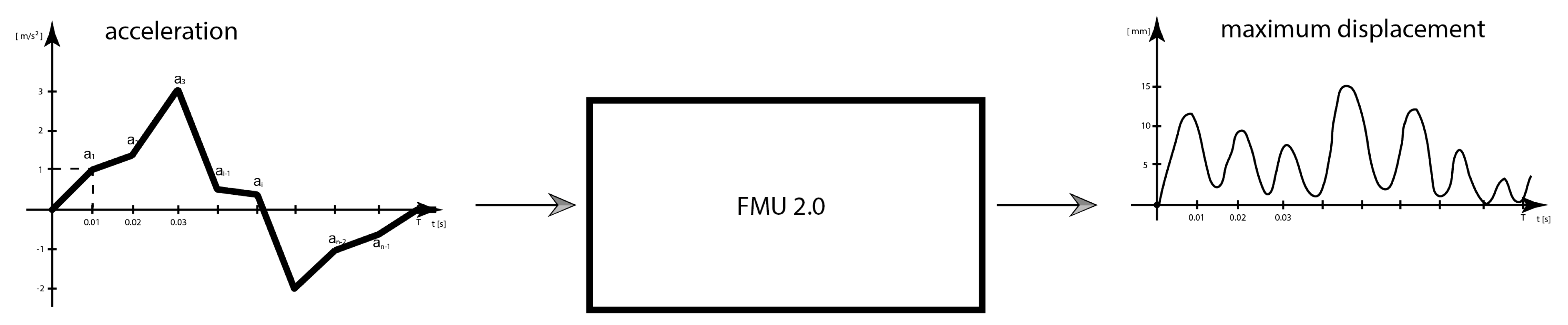
At present, virtual commissioning systems support the FMU 2.0 and FMU 3.0 standards. For our problem, the key difference is that in the case of FMU 2.0 only scalar values can be returned, whereas FMU 3.0 allows matrix-valued outputs. All information about the geometry, material properties, and fixation points must be encapsulated within the model. Thus, we face the task of creating a container that receives the acceleration as an input every 10 milliseconds and, within the next 10 milliseconds, performs the required computations and returns the results.
- for the FMU 3.0 standard, the coordinates of the mesh nodes at the given time step.
- for the FMU 2.0 standard, the maximum deviation among all mesh nodes from their initial positions at the given time step.
Figure 4.
FMU 3.0 with a matrix output
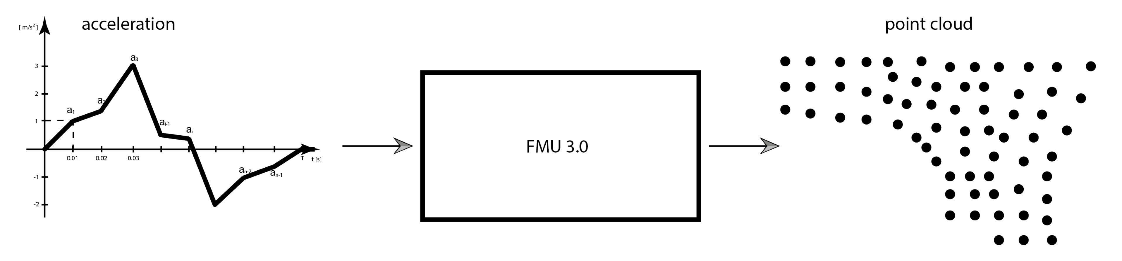
Figure 5.
FMU 2.0 with a scalar output
3. Construction of a Reduced Model
Since our study is focused on the automotive industry, we consider thin components made of structural steel or aluminum alloys. During the stamping process, such parts acquire profiles that act as stiffening ribs and increase their overall bending and torsional stiffness. At the preprocessing stage, FEM simulations can be performed to determine the maximum allowable acceleration threshold that does not lead to plastic deformation of the material under accelerated motion. In addition, industrial robots impose inherent limitations on the maximum TCP velocity and acceleration. These factors allow the vibration dynamics of the flexible part to be treated as linear. The vibration amplitudes of points on the part may reach 20–30 mm for part lengths of 1.5–2 meters, while the stresses arising in the metal do not exceed the plastic deformation threshold.
To remain within the framework of linear dynamics, we consider manipulations without rotation. In this case, the transient analysis can be performed using the modal superposition method (MSUP)[19], which simplifies the preparatory phase of constructing the reduced model. At the same time, the range of applications for non-rotational manipulations remains sufficiently broad, including delta robots, palletizing operations, and the handling of sheet metal parts under a press.
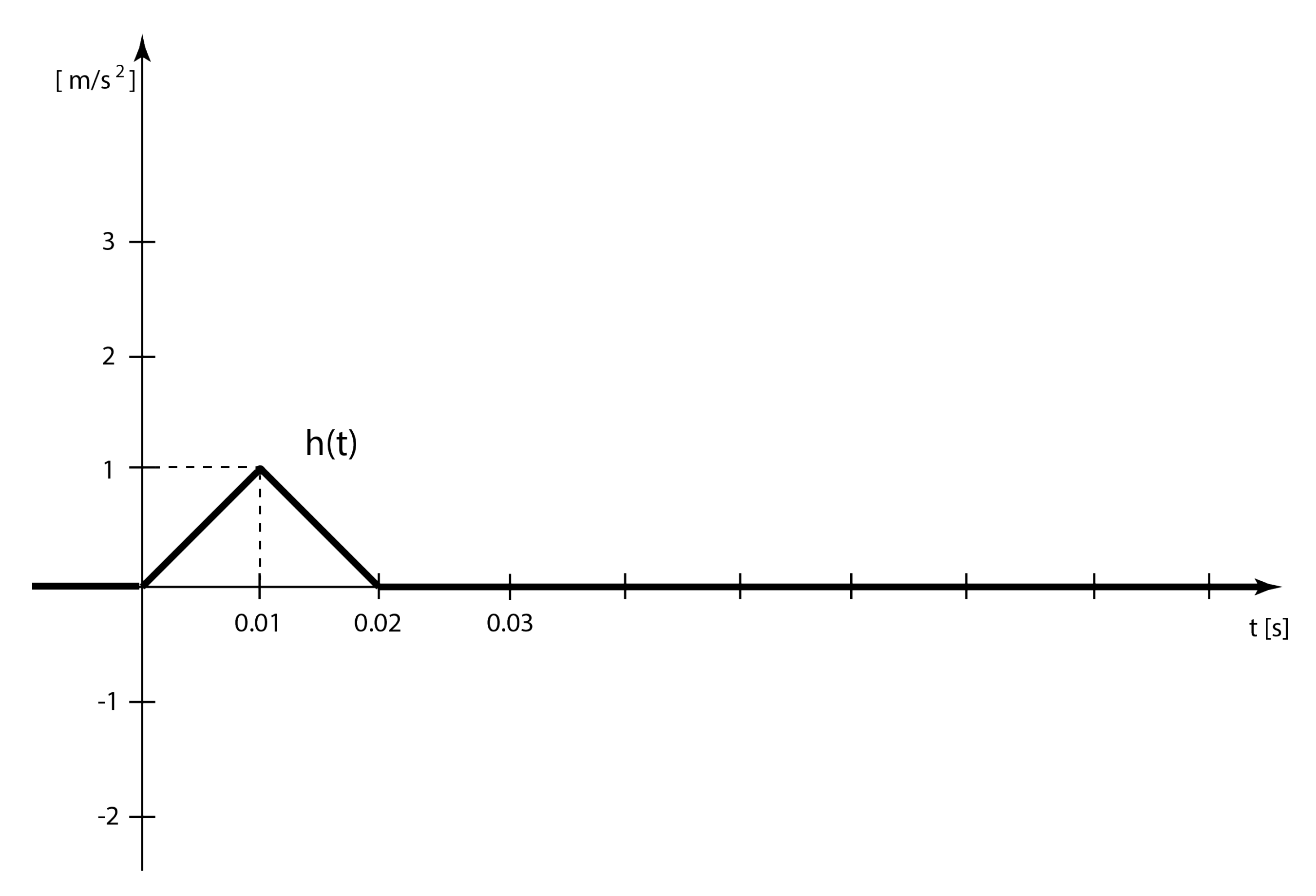
3.1. System Response to a Unit Perturbation
Let us introduce the concept of a unit perturbation constructed for a time step seconds.
Figure 6.
Acceleration profile for a unit perturbation along one of the coordinate axes.
Lemma 1.
The acceleration profile of the form shown in Figure 3, defined by the set of values , can be represented as
The preparatory phase of constructing the reduced model consists in obtaining the dynamic response of the flexible part to an acceleration of the form (1). The results of the transient analysis performed in ANSYS Mechanical are stored as a matrix of displacement vector coordinates for each of the K mesh nodes at each of the N time steps:
For example, for a simulation duration of s with a time step of , and a finite-element mesh consisting of nodes, the resulting matrix has dimensions 50,000×3,000 with elements of type double.
Theorem 1.
The response of the flexible part R to an acceleration of the form shown in Figure 3, defined by the set of values , can be represented as a discrete convolution of the unit response with the sequence , namely:
where the matrix is obtained from the matrix by shifting it three columns to the right, discarding the rightmost elements and filling the leftmost columns with zeros.
At the stage of computing the matrix , the number of mesh nodes and the size of the time step must be chosen so as to ensure high accuracy of the FEM simulation. Subsequently, the number of points can be reduced by tens or even hundreds of times, and the time step can be increased to 20–25 milliseconds in order to accelerate the computations with minimal loss of accuracy.
In the offline phase, a preparatory workflow is carried out, which may take several hours. This includes preparing the CAD model of the flexible part for simulation, generating the finite-element mesh, defining the boundary conditions (fixation at the locations where the part is held by vacuum suction cups), performing a modal analysis with a sufficient number of modes, and subsequently conducting a transient structural analysis based on modal superposition (MSUP).
In this paper, we demonstrate the idea of the method for motion along a single axis. If, however, the acceleration vector has three components at each time step, the application of the method requires three FEM simulations in order to obtain the unit-response matrices , corresponding to unit perturbations along each coordinate axis. The dynamic behavior of the flexible part is then computed according to
It is important to note that constructing surrogate models based on neural networks typically requires hundreds or even thousands of FEM simulations.
3.2. Model Dimensionality Reduction
The construction of the dynamic response of a flexible part to an arbitrary acceleration using our method is implemented as a linear combination of matrices. This means that identical computations are performed independently for each mesh node, which opens up broad opportunities for parallelizing these computations on a GPU.
We carried out a comparative analysis of the computation time for an automotive fender using a mesh composed of 3D tet10 elements with one million nodes. The simulation duration was seconds, corresponding to 300 time steps. At each time step, it was necessary to shift, multiply by a scalar, and sum matrices of size 1,000,000×900. On a CPU, these matrix operations required approximately 15 minutes, while the FEM simulation itself took 18 minutes. In contrast, the same operations on a GPU took only 12 seconds. However, deploying the model in FMU format within virtual commissioning systems requires minimizing external dependencies, such as the need for an NVIDIA GPU to perform CUDA-based computations.
The number of nodes and the size of the time step were of fundamental importance during the FEM simulation stage to achieve high accuracy. At the same time, for demonstrating the dynamic behavior of a flexible part in a virtual commissioning system, it is sufficient to consider only about one thousand points uniformly distributed over the part. In some applications, it is even possible to analyze the behavior of only a few key points, for example, points along the part boundary or at planned fixation locations (welding, bonding), where vibration decay is of greatest interest. This makes it possible to perform all required computations in real time on a CPU.
It should be noted that mesh nodes are distributed non-uniformly over the part, since adaptive meshing leads to higher node density near edges, holes, and bends. Therefore, for uniform node selection, we employed a modified voxel downsampling method commonly used to reduce point cloud density. In each voxel, we selected the mesh node closest to the voxel center and subsequently filtered out nodes that were located closer to each other than a specified distance. The voxel size and the specified minimum distance between nodes were selected manually based on visual inspection to achieve an optimal balance between the number of points and the accuracy of the part representation.
3.3. FMU Packaging
After reducing the number of mesh nodes, one can proceed to the creation of an FMU model. An FMU archive contains two mandatory components: modelDescription.xml, which describes the input and output variables, and library.dll (for Windows), which implements the model logic. In addition, the FMU archive may contain data files. In our case, this is the extended unit response matrix , which contains the coordinates of the displacement vectors of the selected mesh nodes at each time step, as well as the coordinates of these nodes at the initial time instant. Thus, all information about the model geometry and its dynamic behavior is packaged within the FMU model itself in the form of txt, csv, or similar data files.
For a dynamic response of duration seconds with a time step of milliseconds and mesh nodes, this results in a matrix of size 1000×3003 with elements of type double. Let us once again emphasize the difference between the FMU 2.0 and FMU 3.0 standards with respect to the format of the model output data. The choice of the standard is determined by the version supported by the virtual commissioning software. At present, the FMU 2.0 standard is predominantly supported. In this case, the FMU model can return, at each time step, the maximum deviation of the part’s points from their initial positions, which makes it possible to estimate the spatial position of the part while accounting for vibrations, as well as to determine the time instant at which the oscillations have decayed below an admissible threshold and the next technological operation can be initiated.
The FMU 3.0 standard allows for matrix-valued outputs; that is, at each time step, we can return not only the maximum amplitude but also the coordinates of all mesh nodes. This enables realistic real-time visualization of manipulations involving flexible parts.
4. Simulation and Model Accuracy Evaluation
To validate our method, we constructed a dynamic model of an automotive fender based on a CAD geometry provided by an automotive manufacturer. The fender is fixed at four locations, corresponding to the positions of the vacuum suction cups of the gripper. The Figure 7 schematically shows the fender together with the locations of the suction cups.
Since the part measures approximately 1500 mm by 800 mm with a thickness of 1 mm, shell elements of type Shell281 were used for its modeling. A convergence analysis showed that high solution accuracy is achieved with a mesh of 22,000 elements, containing 66,000 nodes. Using solid elements to obtain a stable result would require more than 300,000 nodes. Considering that in reality parts with such complex geometry are produced by press forming and have varying thickness and material properties across different areas, the use of 3D elements may be more justified. Again, we note that in the preparatory phase, FEM simulation accuracy is the priority, so the number of nodes at this stage can reach hundreds of thousands or even millions. To apply the modal superposition method for transient analysis, we first perform a modal analysis and select 40 modes. Figure 8 shows the table of natural frequencies.
Then, based on the MSUP method, we perform a transient analysis with a duration of seconds and a time step of milliseconds. As the load, we use an acceleration of the form (1) along the Y-axis, perpendicular to the plane of the part.
It should be noted that the simulation duration and time step are chosen after a preliminary analysis, when the main natural frequencies are known and the damping time can be estimated with a safety margin for an approximate movement scenario. We also set the damping coefficient In reality, this coefficient depends on various geometric and material properties of the part and should be determined experimentally with high accuracy. It significantly affects the decay time of vibrations and, consequently, the total cycle time.
As a result of the simulation, we obtain the unit response matrix (Table 2).
The part is now represented not as a mesh, but as a point cloud composed of mesh nodes (Figure 9).
It should be noted that if, for a given acceleration profile (Figure 3), the calculations according to (4) are performed for the entire set of mesh nodes, the result will be identical to that obtained from a direct FEM simulation. However, such computations would be far from real-time performance.
To build a fast model, we need to reduce the number of points. For this, we perform voxel downsampling, selecting parameters so that the point set accurately represents the part while keeping the total number of points around 1000 (Figure 10).
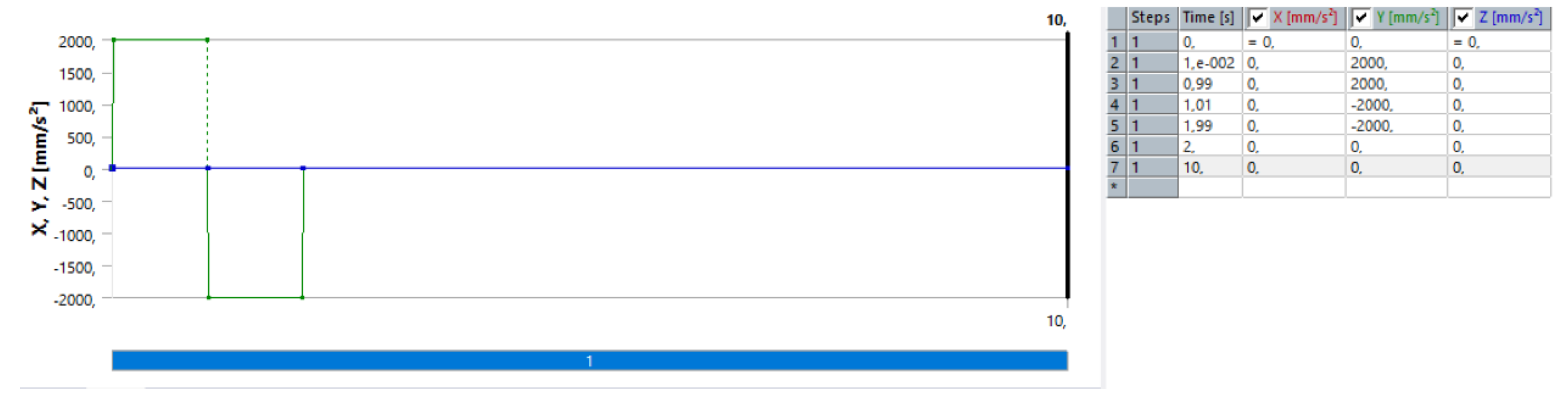
Then, from the unit reaction matrix, we select only those rows corresponding to the chosen points. As a result, we obtain a matrix of size 1099 rows × 3003 columns with elements of type double, which stores the coordinates of the nodes of the reduced mesh and the displacement vector coordinates at each of the 1000 time steps. This matrix, together with the C code implementing the convolution with the acceleration profile (4), is packaged into an FMU file, which contains all the necessary information for computing the flexible part’s behavior in real time. For verification of our model, we performed a transient analysis in ANSYS using the acceleration profile:
Figure 11.
Test disturbance profile
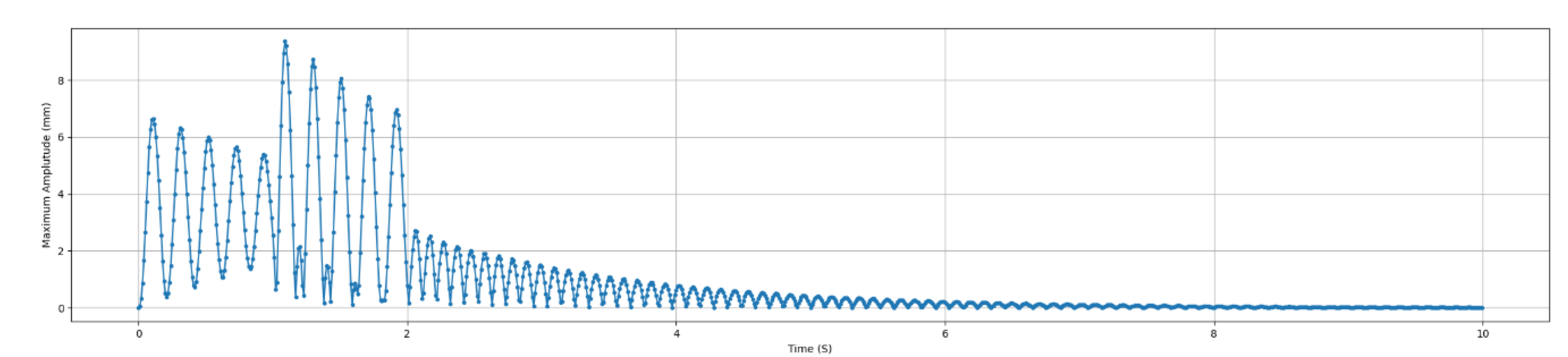
We then compared the maximum amplitudes at each time step obtained from the FEM simulation in ANSYS with those computed using our method.
Figure 12.
Graph of maximum node displacement obtained using the reduced model
We used various metrics for comparison:
which demonstrates the high accuracy of the reduced model. The 0.05 mm discrepancy occurred when comparing the maximum deviations over the entire time: We also determined the time from the start of motion until the oscillations decayed below the threshold value of 0.5 mm. Both models yielded the same value of 4.73 seconds.
Figure 13.
Graph of maximum node displacement based on FEM simulation in ANSYS
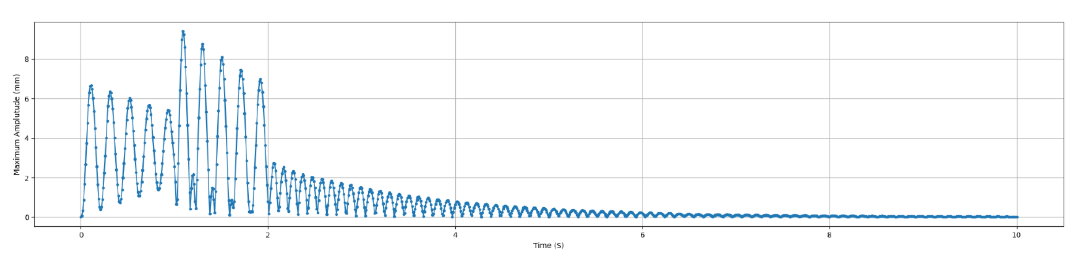
As mentioned earlier, a straightforward reduction of the mesh nodes during the FEM simulation from 66,308 to 1,099 would lead to significant distortion of the results. At the same time, our model reduction approach maintains high accuracy.
On a computer with an Intel Core i7-12800HX processor, 2.0 GHz, and 32 GB of RAM, we evaluated the performance of the reduced model. Generating the graph of maximum amplitude versus time based on the FEM simulation in ANSYS Mechanical took 2 minutes 53 seconds on the CPU. Constructing the same graph using the reduced model took 0.85 seconds on the CPU. Thus, the FMU model, receiving the acceleration value for the next 10 ms, calculates the maximum displacement of the part’s points from their original position in 0.85 ms. This is sufficient for implementing operations with the flexible part in real time within virtual commissioning systems. However, if the reduced model is used to construct an optimal trajectory that minimizes the cycle time for moving the part and the decay of residual vibrations, there is still potential for acceleration using GPU computation.
5. Conclusions
In this work, we demonstrated an approach that enables the integration of robotic manipulations with flexible sheet metal parts into virtual commissioning systems. The main feature of the proposed approach is that the reduced model is built based on FEM simulations conducted on a highly detailed mesh containing hundreds of thousands of nodes, from which only approximately 1,000 representative points are subsequently selected. This allows combining the accuracy of finite element analysis with the ability to perform computations in real time.
In the task of visualizing robotic manipulations with flexible parts, the proposed method outperforms the XPBD method used in the NVIDIA Omniverse environment for modeling the behavior of flexible structures in terms of accuracy. Neural network–based solutions demonstrate significant acceleration in computation time compared to classical FEM, yet they remain too computationally demanding for real-time operation. It is also worth noting that the developed method opens up possibilities for optimizing the robot’s trajectory to minimize the total cycle time, including both the movement of the flexible part and the decay time of residual vibrations at the final position.
Author Contributions
Conceptualization, B.L.; methodology, V.S.; software, V.S.; writing—original draft preparation, V.S.; writing—review and editing, B.L.; All authors have read and agreed to the published version of the manuscript.
Funding
funded by the Deutsche Forschungsgemeinschaft (DFG, German Research Foundation) – 567365885
Data Availability Statement
The original contributions presented in this study are included in the article. Further inquiries can be directed to the corresponding author.
Conflicts of Interest
The authors declare no conflicts of interest.
References
- Jiménez, P. Survey on model-based manipulation planning of deformable objects. Robot. Comput.-Integr. Manuf. CrossRef. 2012, 28(2), 154–163. [Google Scholar] [CrossRef]
- Glorieux, E.; Franciosa, P.; Ceglarek, D. Quality and productivity driven trajectory optimisation for robotic handling of compliant sheet metal parts in multi-press stamping lines. Robot. Comput.-Integr. Manuf. CrossRef. 2019, 56, 264–275. [Google Scholar] [CrossRef]
- Klare, S.; Shramenko, V.; Klingel, L.; Lüdemann-Ravit, B.; Verl, A. Towards Automotive Manufacturing Efficiency: Enhanced Virtual Commissioning Simulation for Dynamic Sheet Metal Handling Optimization. Advances in Automotive Production Technology - Digital Product Development and Manufacturing. SCAP 2024. ARENA2036. Springer, Cham. CrossRef. 2025, 68–75. [Google Scholar]
- Macklin, M.; Müller, M.; Chentanez, N. XPBD: position-based simulation of compliant constrained dynamics. In MIG ’16: Proceedings of the 9th International Conference on Motion in Games, CrossRef. 2016; pp. 49–54. [Google Scholar]
- Li, H.; Ceglarek, D. Optimal Trajectory Planning For Material Handling of Compliant Sheet Metal Parts. J. Mech. Des. CrossRef. 2002, 124(2), 213–222. [Google Scholar] [CrossRef]
- Kudela, J.; Matousek, R. Recent advances and applications of surrogate models for finite element method computations: a review. Soft Comput. CrossRef. 2022, 26, 13709–13733. [Google Scholar] [CrossRef]
- Hoffer, J.G.; Geiger, B.C.; Ofner, P.; Kern, R. Mesh-Free Surrogate Models for Structural Mechanic FEM Simulation: A Comparative Study of Approaches. Appl.Sci. CrossRef. 2021, 11(20), 9411. [Google Scholar] [CrossRef]
- Jayasinghe, S.C.; Mahmoodian, M.; Alavi, A.; Sidiq, A.; Shahrivar, F.; Sun, Z.; Thangarajah, J.; Setunge, S. A review on the applications of artificial neural network techniques for accelerating finite element analysis in the civil engineering domain. Computers and Structures CrossRef. 2025, 310, 107698. [Google Scholar] [CrossRef]
- Triantafyllou, G.; Kalozoumis, P.G.; Dimas, G.; Iakovidis, D.K. DeepFEA: Deep learning for prediction of transient finite element analysis solutions. Expert Systems with Applications CrossRef. 2025, 269, 126343. [Google Scholar] [CrossRef]
- Bastek, J.H.; Kochmann, D. M. Physics-Informed Neural Networks for shell structures. Eur. J. Mech. - A/Solids CrossRef. 2023, 97, 104849. [Google Scholar] [CrossRef]
- Li, T.; Xiao, T. Physics-Informed Neural Network-Based Input Shaping for Vibration Suppression of Flexible Single-Link Robots. Actuators CrossRef. 2025, 14(1), 14. [Google Scholar] [CrossRef]
- Heining, A.; Sawodny, O. Input shaping prefilter for vibration mitigation of distributed parameter system. Mechatronics CrossRef. 2023, 93, 102992. [Google Scholar] [CrossRef]
- Pfaff, T.; Fortunato, M.; Sanchez-Gonzalez, A.; Battaglia, P.W. Learning Mesh-Based Simulation with Graph Networks. Arxiv.org CrossRef. 2020. [Google Scholar]
- Shivaditya, M.V.; Alves, J.; Bugiotti, F.; Magoulès, F. Graph Neural Network-based Surrogate Models for Finite Element Analysis. 2022 21st International Symposium on Distributed Computing and Applications for Business Engineering and Science (DCABES), CrossRef. Chizhou, China, 2022; pp. 54–57. [Google Scholar]
- Gulakala, R.; Markert, B.; Stoffel, M. Graph Neural Network enhanced Finite Element modelling. Proc. Appl. Math. Mech. 2023, 22(1), CrossRef. [Google Scholar] [CrossRef]
- Jiang, C.; Chen, N.-Z. Graph Neural Networks (GNNs) based accelerated numerical simulation. Engineering Applications of Artificial Intelligence CrossRef. 2023, 123(B), 106370. [Google Scholar] [CrossRef]
- Heiland, S.; Klingel, L.; Penter, L.; Jaensch, F.; Schenke, C.; Ihlenfeldt, S.; Verl, A. Virtual Tool Commissioning using LS-DYNA Functional Mock-up Interface. 13th European LS-DYNA Conference, Ulm, Germany, 2021. [Ref. [Google Scholar]
- Modelica Association. Functional Mock-up Interface [Ref].
- Craig, R.R.; Kurdila, A.J. Fundamentals of Structural Dynamics. In Wiley; 2006. [Google Scholar]
Figure 1.
A robot manipulator with a universal gripper and a flexible part
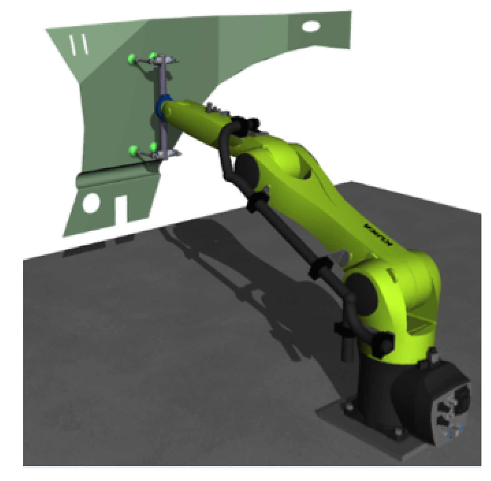
Figure 2.
Dynamic behavior of a flexible part during motion along a prescribed trajectory
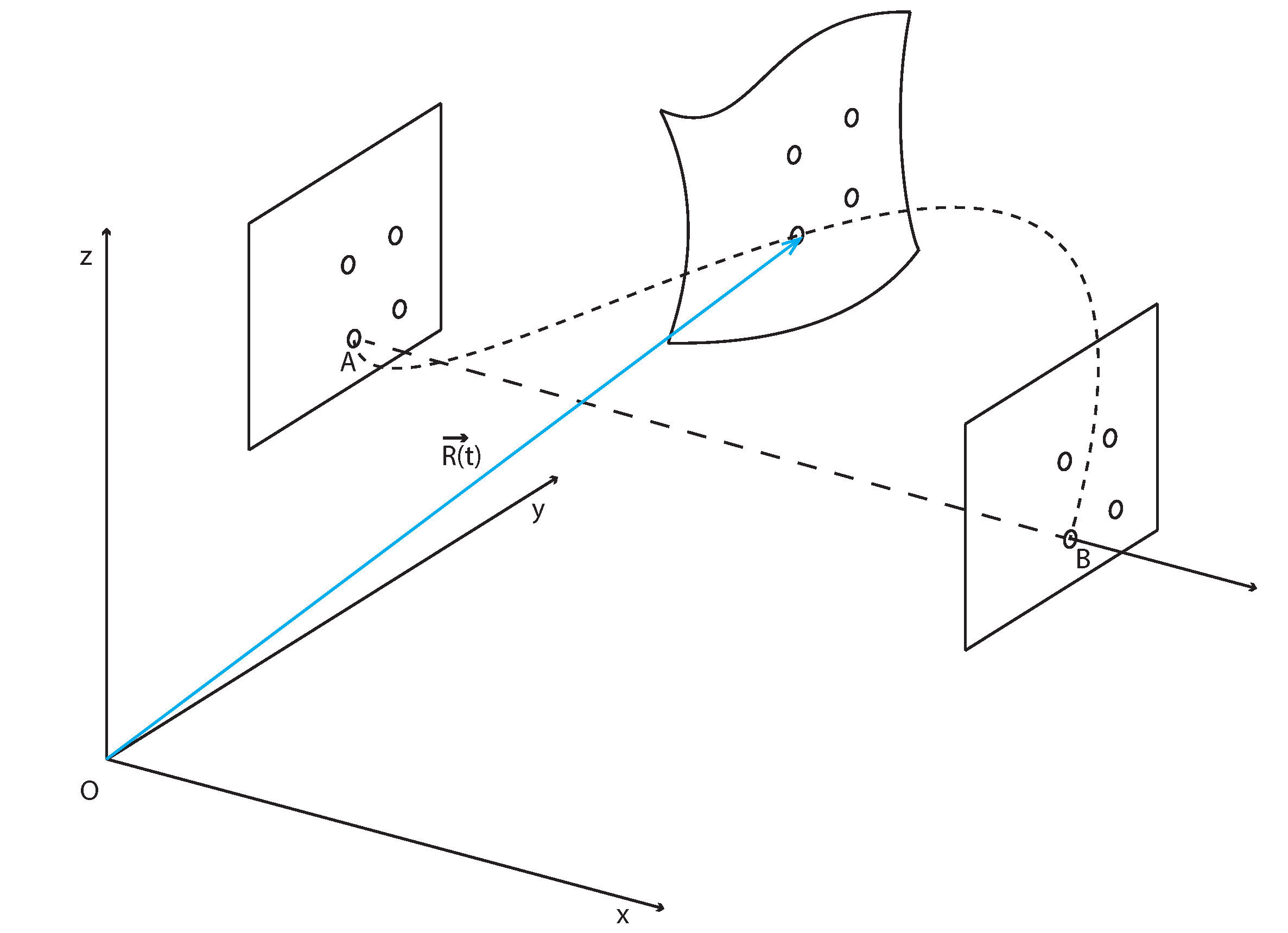
Figure 3.
The acceleration profile along one of the coordinate axes.
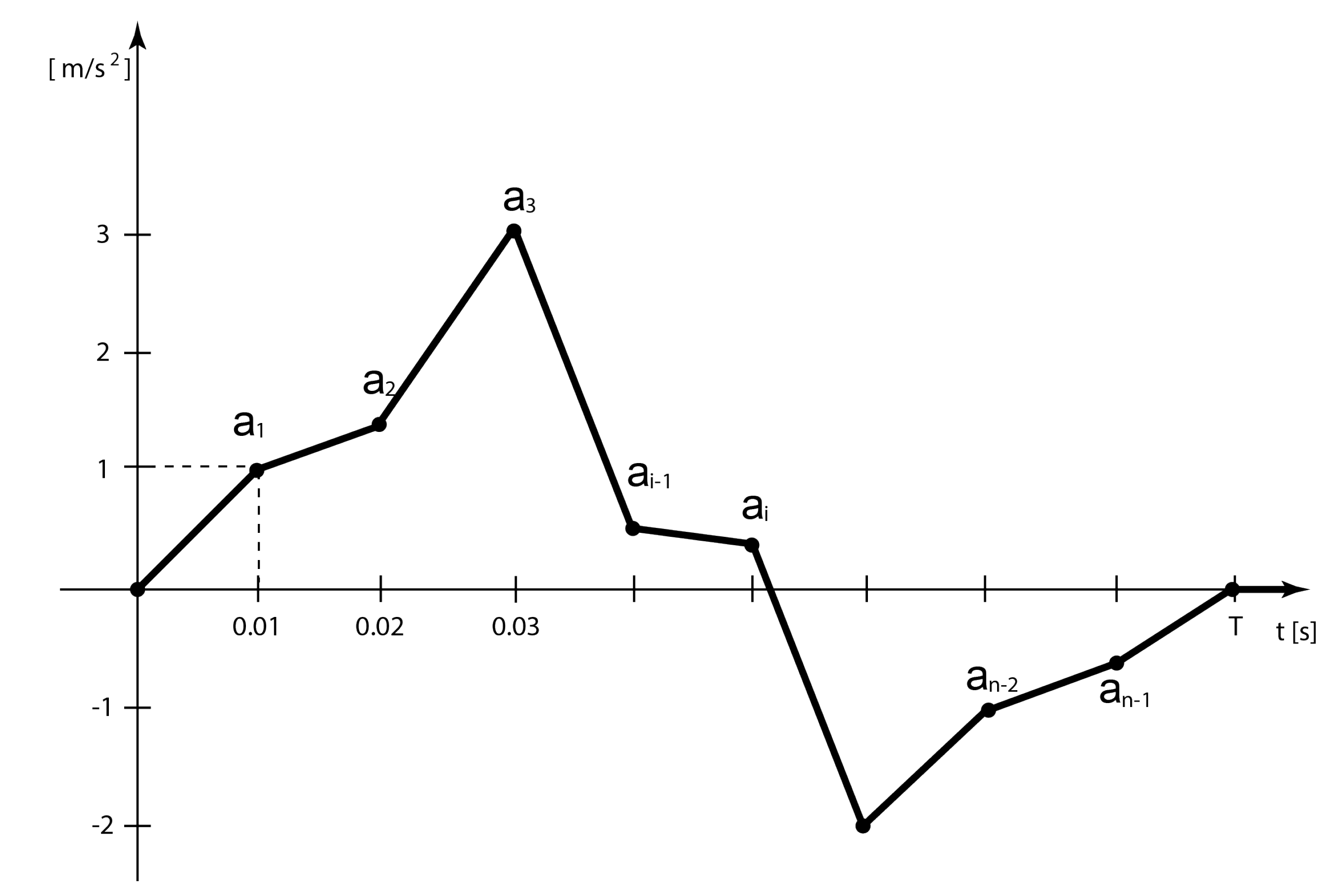
Figure 7.
Schematic depiction of the automotive fender with the mesh and fixation points.
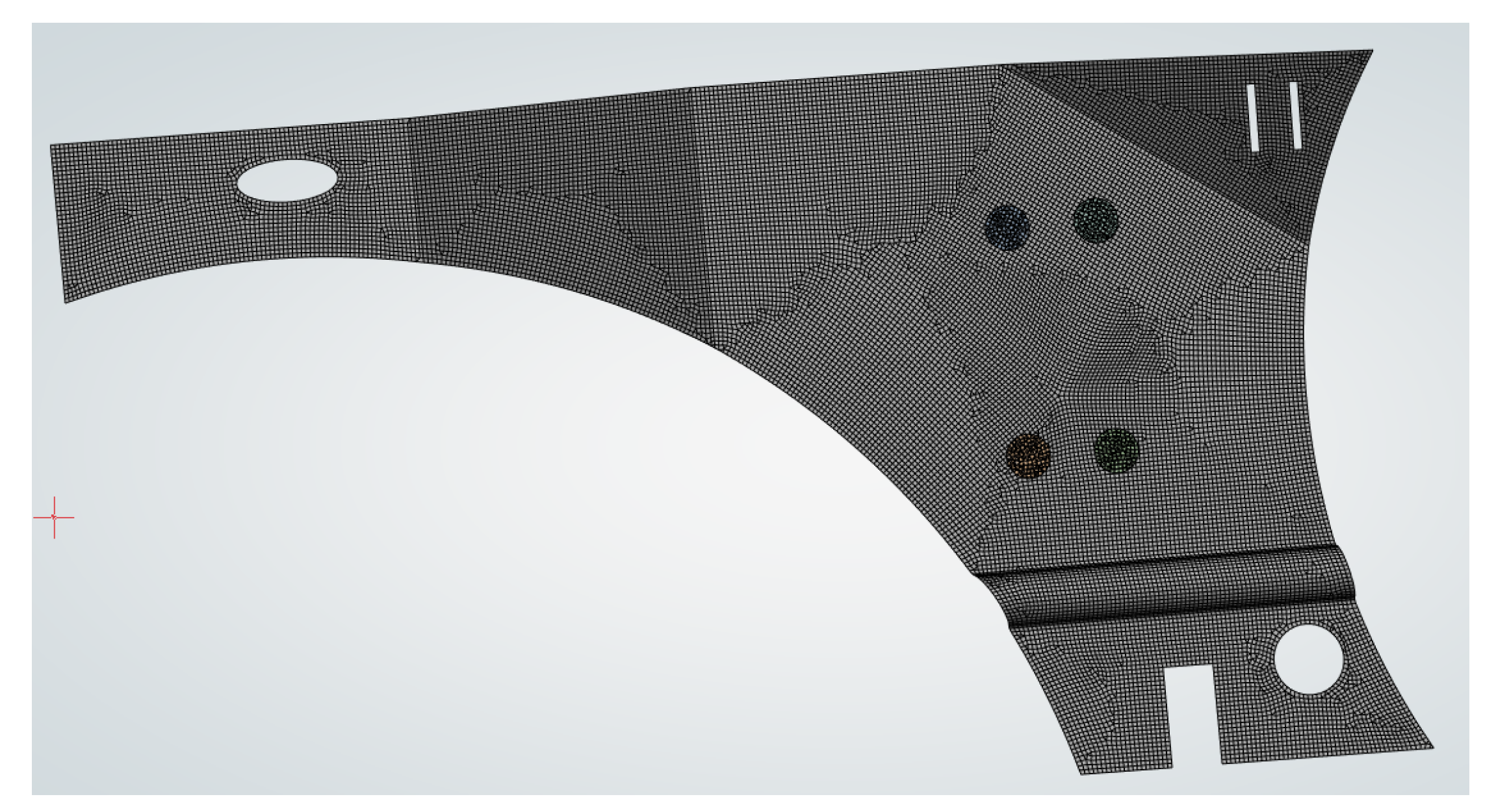
Figure 8.
Natural frequencies obtained from the modal analysis
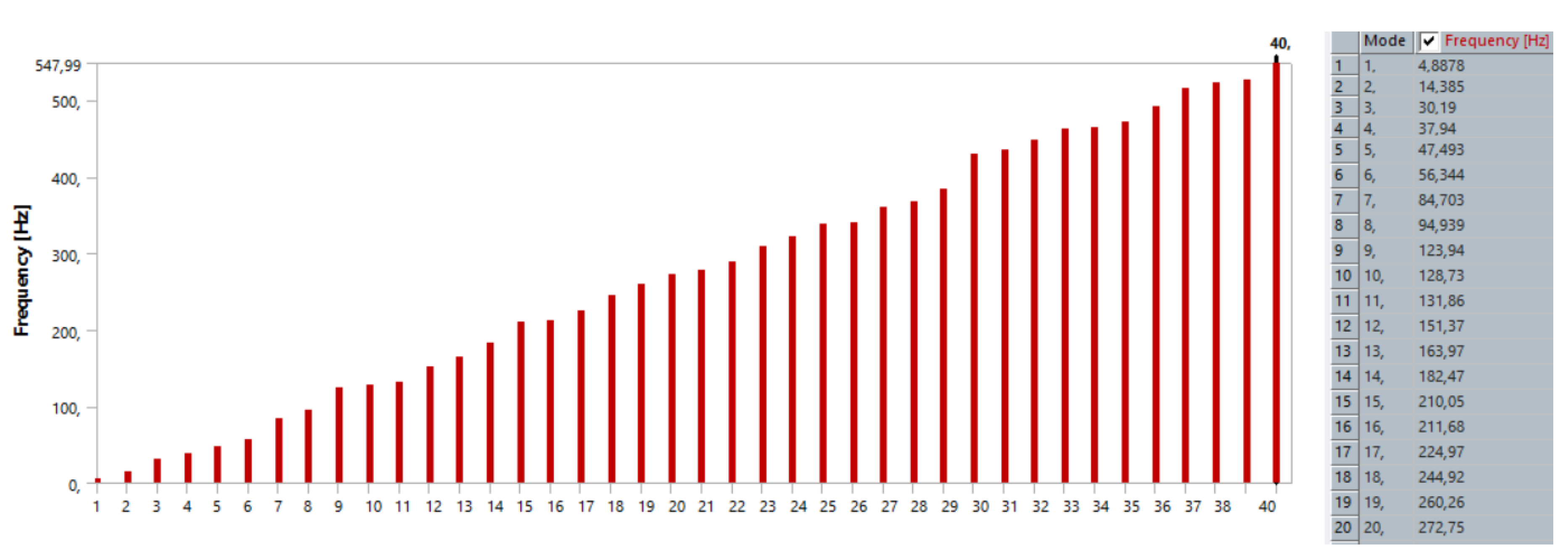
Figure 9.
Nodes of the original mesh
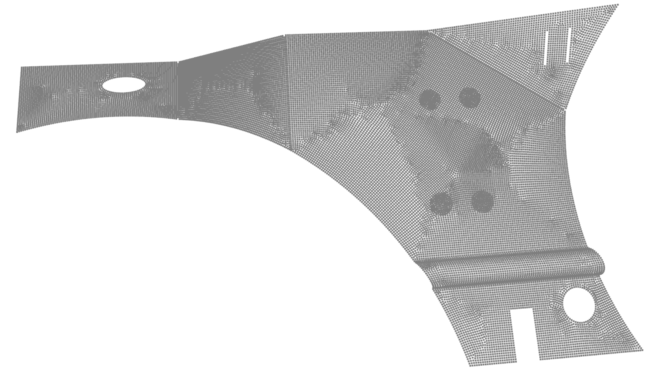
Figure 10.
Reduced set of nodes

Table 1.
Result of the transient analysis: the coordinates of the displacement vectors of each of the K mesh nodes at each of the N time steps.
Table 1.
Result of the transient analysis: the coordinates of the displacement vectors of each of the K mesh nodes at each of the N time steps.
| ... | |||||||
|---|---|---|---|---|---|---|---|
| 1 | ... | ||||||
| 2 | ... | ||||||
| ⋮ | |||||||
| K | ... |
Table 2.
Coordinates of the displacement vectors of each of the 66,308 mesh nodes at each of the 1,000 time steps
Table 2.
Coordinates of the displacement vectors of each of the 66,308 mesh nodes at each of the 1,000 time steps
| ... | |||||||
| 1 | -0.000052 | -0.002547 | 0.000251 | ... | -1.743097e-09 | 1.418202e-06 | -1.095183e-07 |
| 2 | 0.000018 | 0.000835 | 0.000084 | ... | -2.088266e-08 | -7.21781e-07 | -1.307214e-07 |
| ⋮ | |||||||
| 66308 | -0.001802 | -0.022992 | 0.006324 | ... | -3.494957e-05 | -1.287756e-04 | 4.731144e-05 |
Disclaimer/Publisher’s Note: The statements, opinions and data contained in all publications are solely those of the individual author(s) and contributor(s) and not of MDPI and/or the editor(s). MDPI and/or the editor(s) disclaim responsibility for any injury to people or property resulting from any ideas, methods, instructions or products referred to in the content. |
© 2026 by the authors. Licensee MDPI, Basel, Switzerland. This article is an open access article distributed under the terms and conditions of the Creative Commons Attribution (CC BY) license (http://creativecommons.org/licenses/by/4.0/).
Copyright: This open access article is published under a Creative Commons CC BY 4.0 license, which permit the free download, distribution, and reuse, provided that the author and preprint are cited in any reuse.


