Proposed Solution to the Quantum Randi Challenge

1. Introduction

Bell’s Theorem [1] is an important milestone in the history of quantum mechanics. It showed a verifiable statistical difference between compatible and incompatible physical properties. Therefore, it opened a new path of research into the nature of quantum behavior, following the apparent stalemate between Einstein [2] and Bohr [3]. Unfortunately, Bell decided to attach a Locality Criterion to his demonstration, arguing that quantum mechanics is “irreducibly nonlocal”. This claim inspired numerous debates that are still ongoing. Nonetheless, the mathematical correctness of Bell’s Theorem is what influenced the majority view. As a result, contemporary quantum mechanics is defined by its search for exotic solutions to “quantum weirdness” (e.g., non-local pilot waves, super-determinism, parallel universes, etc.). Still, a growing number of independent investigations have been converging on the conclusion that quantum theory is local after all. To list just a few examples, Khrennikov exposed a contradiction between quantum theory and probability theory, if claims of non-locality are taken for granted [4,5]; Cetto and collaborators demonstrated that the bipartite quantum correlation function is local [6,7]; Raymond-Robichaud provided a general proof that any non-signaling phenomenon can be predicted by a local realist theory [9,10]. Accordingly, there are good reasons to reconsider the nature of quantum correlations. Nonetheless, this raises the question: if Bell violations are possible by local means, how do they actually take place? A straightforward answer to this question is proposed below.

The quantum Randi challenge [10,11] is modelled after the paranormal challenge of the James Randi Educational Foundation [12]. The idea is to offer an avenue for impartial validation of an extraordinary claim. Instead of endless debates, with obscure assumptions and elusive conditions, “why don’t you just show us how it works?” Traditionally, many challenges to Bell’s inequality involved complicated statistical effects, aimed at exposing potential loopholes in state-of-the-art experiments. For this reason, Randi-type quantum challenges also involve safeguards against statistical anomalies, provisions for minimal numbers of events, and stipulations about how to design the corresponding computer software for validation. As suggested above, these requirements are influenced by the assumption that the challenge is to falsify Bell’s Theorem. Yet, this is a trap – both for the challengers and for the challenged – because it steers the discussion away from the real problem, which is the overlap between compatible events and local phenomena [13]. The true objective of this challenge is not to falsify what is known, but rather to discover new knowledge. Therefore, the protocol presented below is inspired by the belief that the best demonstration is a simple demonstration. The essence of this pattern is captured by a sequence of 8 events (4 “+” outcomes and 4 “−“ outcomes, given 4 variables). Inspired by Richard Gill’s “wheel of fortune” challenge [14,15], all the events are displayed in a chain that closes on itself. The same pattern is repeated by turning the wheel. Thus, any calculation for large-N trials, be it on paper or in cyberspace, is superfluous. The reason for the maximal Bell violation is made obvious by the arrangement of values on the wheel. The same result is observed by having all the values on a single wheel, or by making two identical copies. In the latter case, the distance between observers is irrelevant, because the final outcome is determined by the printed order of events. The correlations are due to the similarity between the wheels and their patterns of motion. In a nutshell, Bell violations are produced by the temporal arrangement of relevant observables. Such an outcome is logically impossible for events that can take place at the same time.

The following three sections address different aspects of this problem. Section 2 describes the “wheel of fortune” and explains the mechanism behind the maximal Bell violation. Section 3 addresses a few misconceptions about correlated measurements, with regard to differences and similarities between classical and quantum phenomena. Finally, interpretive considerations are discussed in section 4.

2. Maximal Bell violations with staggered events

A simple definition of locality is that isolated events are physically independent from each other. Hence, if Alice and Bob make observations in separate rooms, all of Alice’s events should be the same for any measurement choice by Bob (and vice versa). For example, imagine that Alice decides to measure a binary property A₁, while Bob has a choice between B₁ and B₂. Bob’s events can operate as switches for Alice’s events, such that B₁ produces a “+” for Alice, while B₂ produces a “−“ outcome. In this case, Alice’s observations cannot be explained without action at a distance. Yet, such influences are hard to prove for unpredictable events. Indeed, it was a major breakthrough when Bell demonstrated that simultaneous local events have limited coefficients of correlation for multiple properties and cannot violate predictable bounds [1]. Accordingly, quantum correlations are described as “non-local” because they violate Bell-type inequalities. The problem is that such violations are only possible when measuring incompatible quantum properties. It has been an open question whether mutually exclusive observables are covered by Bell’s demonstration or not [13].

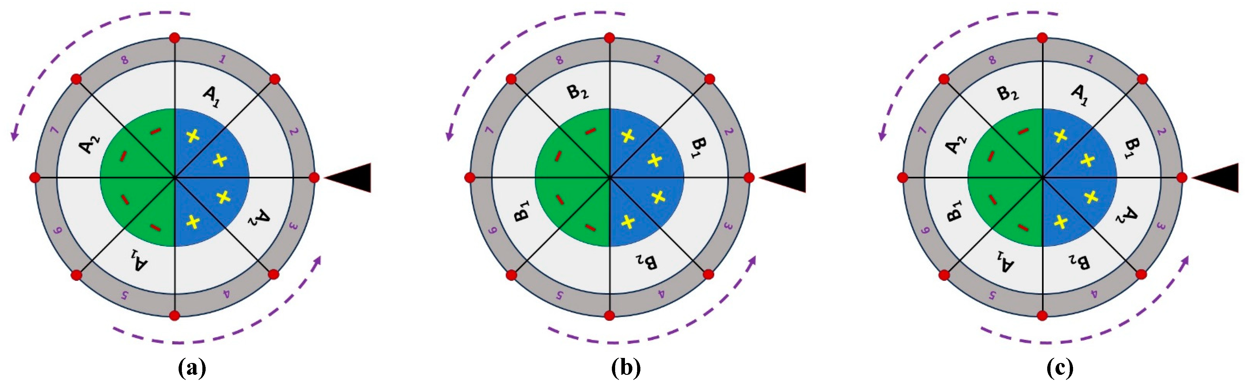
In practical terms, the obstacle is intuitive: how is it possible to satisfy locality without simultaneous observables? As shown above, Alice’s events should be the same, no matter what Bob does. Bob’s events must also be the same, no matter what Alice does. This means that A₁ (or A₂) events should be identical in combination with B₁ and B₂, and vice versa. Therefore, it appears that local events can only happen at the same time (or, at least, their manifestation should be compatible, such that they can be recorded on the same line of a table). Surprisingly, this is not always the case. A possible solution is shown in Fig. 1c, where four “+” values and four “−“ values are printed in sequence on a “wheel of fortune”. Every Alice event is flanked by two alternative Bob events. Therefore, Alice’s events are fixed, regardless of Bob’s choice of observation. The same is true for Bob. However, it is a necessary feature of this arrangement that B₁ and B₂ values cannot be adjacent to the same value of A₁. Therefore, unusual correlations are possible: A₁ is correlated with B₁, B₁ with A₂, and A₂ with B₂, but B₂ and A₁ are anti-correlated. The direct consequence of this arrangement is a maximal Bell violation, as explained below.

A Bell-type experiment requires two copies of the same wheel. Alice may get a version with Bob’s values removed, as shown in Fig. 1a, while Bob can receive a copy with Alice’s values removed (Fig. 1b). Alice and Bob can be arbitrarily close or far from each other. The only requirement is that the motion of their wheels is perfectly synchronized. Accordingly, two kinds of “Bell games” are possible:

Game 1: Complete measurement. Alice and Bob record all of their events with exact timestamps, as they pass by the pointer on the right side of the table, continuously. This can be done automatically, with machines supervised by Alice and Bob. Of course, Alice and Bob can also do this with pen and paper (and slower speeds of rotation for the tables). After accumulating sufficiently large data sets, Alice and Bob can meet to reconcile their events (by hand, or on a computer). For a fixed rate of rotation of 1 turn per second, they must post-select all the pairs of events that happen within 1/8 of a second from each other. This way, they can isolate the coincidences between (A₁, B₁), (A₁, B₂), (A₂, B₁) and (A₂, B₂).

Game 2a: Random measurement. The tables of Alice and Bob are hardwired to move and stop in perfect unison. Either player (or a moderator) can start the synchronous motion, while a random mechanism causes the tables to stop in a manner that cannot be predicted by the players. The wheels are also hardwired to end every turn on identical red dots (on the line between two adjacent sectors). Every time, Alice and Bob must record the nearest observable to the “winning” stop point, with the “+” or “−” value that happens to be in the same sector. After accumulating a sufficiently large number of events, they can reconcile their lists and determine the coefficients of correlation for each pair.

Game 2b: Random sampling. Alice and Bob repeat the same procedure as in Game1. They record all the events, as they happen in sequence, for a pre-arranged duration. Then, Alice and Bob reunite to compare outcomes. They use random number generators to choose combinations of variables and random segments of time to post-select coincidences (within 1/8 s) from the two records of events. This is not fundamentally different from Game 2a, since the full structure of the game is deterministic.

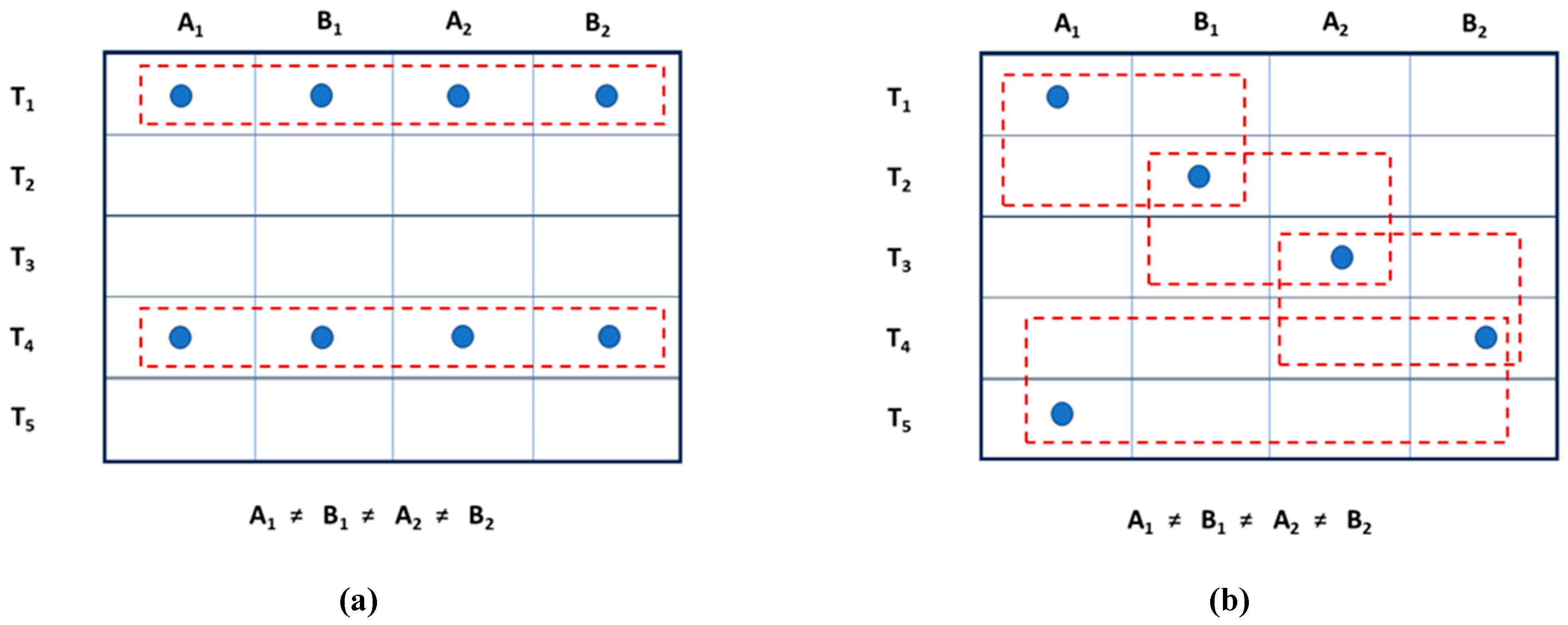
All of these games are expected to have the same result: a maximal violation of the CHSH inequality [16]. Indeed, the random games are superfluous. They are only needed when complete measurements are not possible. Deviations between Games 2 and Game 1 are not likely, except in the case of equipment malfunction. Barring loss of synchronicity, the order of events is fixed, and statistical anomalies are not possible even for low numbers of repetitions. The bottom line is that Bell violations are the correct theoretical outcome. The reason for this type of behavior is easy to grasp intuitively. When several properties occur at the same time (as shown in Figure 2a), they obey the so-called transitive rule. For example, if we have three observables X, Y, and Z, then two correlations automatically determine the third. If X is correlated with Y, and Y is correlated with Z, then X is correlated with Z as well. For illustration, consider a pile of shirts, such that “all the white shirts are made from cotton” and “all the cotton shirts are short-sleeved”. It is logically necessary that “all the white shirts are short-sleeved” in the same group. It would be a contradiction to have even one white shirt with long sleeves. Accordingly, Bell violations are logically impossible because they entail contradictory properties for one and the same object. In contrast, when we have mutually exclusive events that are staggered in time, the transitive rule does not apply. Instead, pairwise detections are restricted to adjacent events (Figure 2b), preventing the coincidence of B₁ and B₂ with the same event for A₁. Therefore, it is no longer a contradiction to have correlations and anti-correlations for the same set of observables.

Figure 1. Bell experiment with correlated spinning tables. Two players, Alice and Bob, supervise the flow of events on synchronized “wheel-of-fortune” devices without interfering. The table surface is divided into 8 sectors, with 4 “+” events followed by 4 “−” events, as shown in image (c). These values correspond to 4 observables, as needed for a Bell experiment that follows the CHSH protocol. Alice’s table (a) has empty sectors for Bob’s observables, while Bob’s table (b) is missing Alice’s observables. The tables are hardwired to move and stop in perfect unison. A “game host” can start the synchronous rotation, while a random mechanism forces the wheels to stop together at one of the 8 red dots. The players record the values of the observable adjacent sectors (A1 or A2 for Alice, and B1 or B2 for Bob). The goal is to analyze the correlation between coincident events, after playing the game long enough for statistical significance. Yet, the outcome is obviously predetermined. Of the 4 pairwise combinations – (A1,B1), (B1,A2), (A2,B2) and (B2, A1) – three are always correlated and one is always anti-correlated. The final result is a maximal violation of the CHSH inequality (S=4), as shown on page 5. This confirms the equivalence between non-signaling and local phenomena in both classical and quantum physics.

Figure 1. Bell experiment with correlated spinning tables. Two players, Alice and Bob, supervise the flow of events on synchronized “wheel-of-fortune” devices without interfering. The table surface is divided into 8 sectors, with 4 “+” events followed by 4 “−” events, as shown in image (c). These values correspond to 4 observables, as needed for a Bell experiment that follows the CHSH protocol. Alice’s table (a) has empty sectors for Bob’s observables, while Bob’s table (b) is missing Alice’s observables. The tables are hardwired to move and stop in perfect unison. A “game host” can start the synchronous rotation, while a random mechanism forces the wheels to stop together at one of the 8 red dots. The players record the values of the observable adjacent sectors (A1 or A2 for Alice, and B1 or B2 for Bob). The goal is to analyze the correlation between coincident events, after playing the game long enough for statistical significance. Yet, the outcome is obviously predetermined. Of the 4 pairwise combinations – (A1,B1), (B1,A2), (A2,B2) and (B2, A1) – three are always correlated and one is always anti-correlated. The final result is a maximal violation of the CHSH inequality (S=4), as shown on page 5. This confirms the equivalence between non-signaling and local phenomena in both classical and quantum physics.

As a reminder, the CHSH inequality [16] for this type of joint measurements is:

$$S=\left|E\left(A_1,B_1\right)-E\left(A_1,B_2\right)+E\left(A_2,B_1\right)+E\left(A_2,B_2\right)\right|,$$

where

$$E\left(X,Y\right)=\frac{P\left(X^{+},Y^{+}\right)+P\left(X^{-},Y^{-}\right)-P\left(X^{+},Y^{-}\right)-P\left(X^{-},Y^{+}\right)}{P\left(X^{+},Y^{+}\right)+P\left(X^{-},Y^{-}\right)+P\left(X^{+},Y^{-}\right)+P\left(X^{-},Y^{+}\right)}=\frac{P\left(\mathrm{same}\right)-P\left(different\right)}{P\left(total\right)}.$$

As described in the game, coincidence windows allow exclusively for (+,+) and (-,-) observations between three variables. Hence,

$$E\left(A_1,B_1\right)=E\left(B_1,A_2\right)=E\left(A_2,B_2\right)=\frac{100-0}{100}=1.$$

In contrast, the remaining pair is always anticorrelated, since it can only display (-,+) and (+,-) coincidences:

$$E\left(A_1,B_2\right)=\frac{0-100}{100}=-1.$$

Accordingly, the final tally is:

$$\begin{array}{c}S=\left|1-\left(-1\right)+1+1\right|\\ S=4.\end{array}$$

This conclusion resonates with an interesting open question in quantum theory. It is well-known that quantum behavior is “non-signaling”, but can it be “non-signaling” and “non-local” at the same time? As shown by Popescu and Rohrlich [17], non-signaling events allow for maximal Bell violations (up to S=4), far beyond the known limits of quantum correlations. More recently, Raymond-Robichaud demonstrated the equivalence between local realism and non-signaling behavior [8, 9]. In other words, any non-signaling phenomenon can be predicted by at least one local realist theory. The solution described above supports this conclusion, with an important difference: Bell violations are produced by staggered events in the same universe, as opposed to simultaneous events in parallel universes. Therefore, “super-quantum” correlations are not just “local” and “realist”. They are ordinary classical phenomena.

Furthermore, such effects are possible with pairwise joint events, but not necessarily with larger numbers of simultaneous detections. For example, if Alice and Bob are instructed to record single values for two variables (each) at the same time, at random points in time, then they end up producing isolated groups of four events, just like in Figure 2a above. As a result, the four different values are forced to become compatible, erasing the effect of temporal mismatch between them. In this case, Bell violations are no longer possible. Therefore, “quantum monogamy” [18] is also an ordinary classical phenomenon.

3. Pairwise correlations demystified

A curious feature of typical Bell experiments is that measurement correlations are rotationally invariant (for electron spin or photon polarization settings). This observation puzzled numerous interpreters, struggling to find classical explanations for this type of phenomena, and probably hindered the understanding of quantum entanglement in general. Indeed, the solution presented above was made possible by a moment of epiphany concerning the difference between “invariant events” and “invariant correlations”. The pitfall is the temptation to rely on intuitions about the former for the interpretation of the latter. The easiest way to clarify this difference is by imagining a simple sequence of events, such as when an observer has three light bulbs with the ability to switch any one of them ON or OFF independently. For a set of “correlation games”, two observers (Alice and Bob) receive their own set of three lights. The goal is to test the effect of various rules of transformation on the correlations between the two sets. Some combination patterns are presented below, in order to help the analysis of relevant misconceptions about this topic.

Misconception #1: Identical measurements are by default non-local if they are rotationally invariant. Bell experiments involve mutually exclusive properties. Only one property can be real at time. Yet, any measurement choice results in a perfect correlation. How can Alice’s quantum “know” which property was chosen by Bob, in order to “collapse” in the adequate identical state?

The key to this puzzle is to shift the focus from individual events (which cannot be fixed in advance) to coefficients of correlation (which can be stable under identical transformations). Consider the following correlation games.

Game 1. Starting distributions: (0, 0, 0) for Alice and (0, 0, 0) for Bob. Perfect correlation. Transformation rule: “Flip all the lights to their opposite state”. Final distributions: (1, 1, 1) for Alice and (1, 1, 1) for Bob. Perfect correlation.

Game 2. Starting distributions: (1, 1, 1) for Alice and (1, 1, 1) for Bob. Perfect correlation. Transformation rule: “Flip light #2 for both players”. Final distributions: (1, 0, 1) for Alice and (1, 0, 1) for Bob. Perfect correlation.

Game 3. Starting distributions: (0, 1, 1) for Alice and (0, 1, 1) for Bob. Perfect correlation. Transformation rule: “Flip lights #1 and #3 for both players”. Final distributions: (1, 1, 0) for Alice and (1, 1, 0) for Bob. Perfect correlation.

Conclusion: The starting distributions do not matter, and the rules of transformation do not matter, as long as they are identical for both players. The outcomes are different in each game, but the correlations are invariant. Rotationally invariant correlations for identical measurements are a classical phenomenon.

Misconception #2. Non-identical quantum observations are intrinsically non-local. Alice’s quanta cannot know the state of Bob’s quanta, yet the final correlation is only dependent on the angle between the measurement settings in Bell experiments.

The antidote is found, again, with correlation games.

Game 4. Starting distributions: (0, 0, 0) for Alice and (0, 0, 0) for Bob. Perfect correlation. Transformation rules: “Alice flips light #1. Bob does nothing”. Final distributions: (1, 0, 0) for Alice and (0, 0, 0) for Bob. Difference between the rules: 1/3. Difference between distributions: 1/3.

Game 5. Starting distributions: (1, 0, 0) for Alice and (1, 0, 0) for Bob. Perfect correlation. Transformation rules: “Alice does nothing. Bob flips light #2”. Final distributions: (1, 0, 0) for Alice and (1, 1, 0) for Bob. Difference between the rules: 1/3. Difference between distributions: 1/3.

Game 6. Starting distributions: (1, 1, 0) for Alice and (1, 1, 0) for Bob. Perfect correlation. Transformation rules: “Alice flips light #1. Bob flips light #3”. Final distributions: (0, 1, 0) for Alice and (1, 1, 1) for Bob. Difference between the rules: 2/3. Difference between distributions: 2/3.

Conclusion: The details of the starting distributions do not matter, as long as they are identical. The details of individual rules do not matter for the final result. The only relevant factor is the difference between the two rules of transformation. Rotational invariance of coefficients of correlation for non-identical measurement is also a classical phenomenon.

Misconception #3. Consecutive measurements of the same system influence each other directly. This is why parallel measurements with correlated systems require action at a distance when they exhibit identical behavior. (This is in reference to classical measurements of polarization that are known to violate Bell-type inequalities [19]).

In this case, each correlation game needs to be repeated twice, with parallel and sequential changes.

Game 7a. Starting distributions: (0, 0, 0) for Alice and (0, 0, 0) for Bob. Perfect correlation. Transformation Rules: “Flip light #1 for Alice. Flip light #1 for Bob”. Final distributions: (1, 0, 0) for Alice and (1, 0, 0) for Bob. Perfect correlation.

Game 7b. Starting distributions: (0, 0, 0) for Alice and (0, 0, 0) for Bob. Perfect correlation. Transformation rules: “Flip light #1 for Alice. Flip light #1 for Alice again, instead of Bob). Final distributions: (0, 0, 0) for Alice and (0, 0, 0) for Bob. Perfect correlation.

Game 8a. Starting distributions: (1, 1, 1) for Alice and (1, 1, 1) for Bob. Perfect correlation. Transformation Rules: “Flip #1 for Alice. Flip #2 for Bob”. Final distributions: (0, 1, 1) for Alice and (1, 0, 1) for Bob. Difference between the rules: 2/3. Difference between event distributions: 2/3.

Game 8b. Starting distributions: (1, 1, 1) for Alice and (1, 1, 1) for Bob. Perfect correlation. Transformation rules: “Flip #1 for Bob, instead of Alice. Flip #2 for Bob”. Final distributions: (1, 1, 1) for Alice and (0, 0, 1) for Bob. Difference between the rules: 2/3. Difference between distributions: 2/3.

Conclusion: If does not matter if the transformations are identical or different for Alice and Bob. Consecutive measurements (over a single system) produce the same relative effects as parallel measurements (over two systems). The outcomes are different, because remote events do not influence each other, but the coefficients of correlation are identical in the two scenarios. Consecutive and parallel events are both local, without direct influences between measurement settings. The rules of transformation are sufficient to explain the outcome.

Objection #1. Quantum measurements are performed by measurement devices without intervening transformations. They are different from the correlation games described above. For example, consecutive measurements of polarization are performed with two polarizing beam-splitters (PBS) in sequence. Real experiments require direct influences between measurement devices.

Response. Measurement devices are more complicated than generally acknowledged. For example, PBS cubes involve an initial stage of propagation through a birefringent medium, followed by a beam-splitting effect at a semi-reflective surface. In the limit, different measurements perform the same function: they determine the ratio of transmitted to reflected quanta. Yet, they are different when they are preceded by different transformations.

For example, optical experiments are challenging, when beams are not parallel to the bench. Rotating a beam-splitter could direct a beam into the ground, or high into the air. Instead, consecutive measurements are often performed by aligning all the PBS cubes in the same plane (with horizontal fast axis). Finally, half-wave plates are inserted in-between and rotated as necessary, to produce required shifts in polarization. (This is common practice. See, for example, reference [20]). Hence, the correct sequence of operations in this case is: <Measurement> followed by <Transformation> followed by <Repeat the same measurement>. The transforming device (in this case, the half-wave plate) can be arbitrarily close or far from the second PBS, other things being equal, just like the operation of switching lights in the described correlation games. The exact coordinates of each transformation do not matter for the final result. Consequently, it is misleading to interpret the effect of consecutive (or parallel) observations in terms of direct influences between measurements. The reason for the relevant coefficients of correlation is found in the relationships between the transformations that precede the measurements and can be physically independent from them.

Objection #2. Photon polarization measurements always obey Malus Law, which is known to operate on linear sharp states. Yet, single photons can express superpositions of multiple vectors, according to quantum mechanics. Therefore, quanta need to collapse to sharp states in Bell experiments, and they also need non-local interactions to coordinate “joint collapse” in the case of entangled photons. If not, how do they express Malus’ Law in Bell experiments?

Response: Malus’ Law does not govern individual outcomes. It is a statistical law the describes correlations. To be more precise, it defines a relationship between coefficients of correlation and angular differences between measurement settings. As shown with the correlation games above, this relationship may seem counterintuitive, if analyzed with improper assumptions. In the final analysis, the values of coefficients of correlation are not anchored on particular input parameters or individual rules of transformation. They only depend on the difference between the rules of transformation that precede individual measurements. Accordingly, Malus’ Law was discovered with sharp states of linear polarization, where the patterns are easier to observe. However, this should be interpreted as a particular instance of a more general law. In other words, it does not matter if the photons are prepared with sharp states of polarization or not. The angular difference between measurement settings is the only parameter that qualifies as an essential feature of Malus Law.

To sum up, quantum correlations and classical correlations may seem equally daunting on the surface, but they share a surprisingly simple underlying mechanism, without any kind of “non-classical” magic. The special nuance is to keep in mind the difference between events and correlations. What may seem “weird” for one is perfectly normal for the other.

4. Discussion

Quantum mechanics and classical mechanics are connected by the Correspondence Principle. This means that quantum statistics cannot contradict classical statistics for large numbers of events. In the limit, quantum behavior is randomized classical wave behavior, recodified in the discrete regime. As seen in many experiments with binary outcomes, the proportion of wave energy that is transmitted/ reflected corresponds to the proportion of detectable quantum events that appear transmitted/reflected. Therefore, it makes sense to start untangling the mystery of quantum correlations at the classical level, where mechanical clues are more readily available for consideration [19]. Hence, every Optics textbook includes a discussion about polarization measurements and their incompatibility (usually, with a sequence of 2-3 polarizing filters). It is well known that classical beams obey Malus’ Law, and it is known that such a law entails strange outcomes, but it was never appreciated just how strange this really was, prior to Bell’s Theorem. The real puzzle is interpretive: how is it logically possible for such incompatible outcomes to emerge from one and the same optical projection? Yes, real beams express this behavior all the time. Yes, we can measure it and record values on paper. Nonetheless, how can these values be reconciled with each other in a manner that makes sense? In retrospect, the answer is to trace the physical history of this process in reverse. Beam profiles become incompatible after passage through polarizing filters. What do these filters do? On closer inspection, they do two things: they rotate the plane of polarization of an input projection and (!) introduce phase-delays. Which of these two properties is ignored more often? Maybe, that is the missing piece of the puzzle?

As shown above, maximal Bell violations are possible when the phase delay between any two measurements is constant, such that any combination of two observables can be detected within the same coincidence window. Furthermore, positive (negative) values have to be grouped together, ensuring maximal coefficients of correlation between adjacent events. Finally, the largest violations are possible when there is a sudden shift from the positive to the negative domain (and vice versa), emphasized with different colors on the “wheel of fortune”. There is an instructive difference between the solution presented above and the known features of actual spin-like measurements. First of all, there is a gradual increase in phase delay between optical components, as the angle between polarization measurements is increased. Real Bell experiments had to force a constant delay by choosing four measurements at equal angular intervals from each other. Secondly, rotations of the plane of polarization introduce a gradual (and non-linear) loss of correlation, as dictated by Malus’ Law. This explains the gap between the maximal Bell violations that are numerically possible and the ones that are theoretically possible for wave-functions. From the perspective of Bell’s argument, the apparent problem was that quantum correlations were “too high”. Yet, as suggested by Popescu and Rohrlich [17], the true physical puzzle was that they were “too low”. As shown above, there is nothing special or non-classical about Bell violations, be they “quantum” or “super-quantum”. Indeed, it is misleading to call these correlations “quantum”, because they are natural properties of classical beams as well.

Another favorable condition for discovering this solution was the decision to treat “quantum nonlocality” and “quantum monogamy” as a single problem. It would not work to solve just one and hope to patch the other later. Under the influence of real details from loophole-free experiments, an earlier proposal was to consider possible correlations between simultaneous random events, modulo the probability of coincidence [18]. Intuitively, single events are more probable than double events, which are more likely than triple events, and so on. This explained the emergence of incompatible pairs of events, with quantum monogamy as a subset of this pattern. Unfortunately, such a solution could not work for classical projections, where Bell violations and “Bell monogamy” are both possible for ideal measurements, without down-selection or loss of energy. Indeed, as shown above, a better solution was waiting to be found. This shows that quantum experiments are not always the best way to get insights on quantum behavior. Decades of debates about “loopholes” confirm that. Sometimes, the best way to understand quantum behavior is by studying classical wave mechanics, while keeping in mind that it is still a work in progress.

Finally, it should be noted that the original Randi challenge was designed to weed out attempts at deceiving the public with supernatural claims. Ironically, the quantum Randi challenge was formulated to protect a supernatural claim (“quantum non-locality”) against sustained attempts to demystify it. Indeed, the dominant attitude in the community has been that “local realism” is pseudoscience. This placed a stigma on any qualified effort to advance research in this direction. Given the simplicity of the solution proposed above, it might be appropriate to question the wisdom behind this social pressure. It is hard to imagine that the hypothesis of quantum non-locality would have survived for so long if the playing field was level for all the relevant approaches to this problem.

References

- Bell, J.S. Speakable and unspeakable in quantum mechanics (Cambridge UP, 1987).
- Einstein, A.; Podolsky, B.; Rosen, N. Can Quantum-Mechanical Description of Physical Reality Be Considered Complete? Phys. Rev. 1935, 47, 777. [Google Scholar] [CrossRef]
- Bohr, N. Can Quantum-Mechanical Description of Physical Reality Be Considered Complete? Phys. Rev. 1935, 48, 696. [Google Scholar] [CrossRef]
- Khrennikov, A. Bell-Boole Inequality: Nonlocality or Probabilistic Incompatibility of Random Variables? Entropy 2008, 10, 19. [Google Scholar] [CrossRef]
- Khrennikov, A. Get Rid of Nonlocality from Quantum Physics. Entropy 2019, 21, 806. [Google Scholar] [CrossRef] [PubMed]
- Cetto, A.M.; Valdés-Hernández, A.; de la Peña, L. On the Spin Projection Operator and the Probabilistic Meaning of the Bipartite Correlation Function. Found. Phys. 2020, 50, 27. [Google Scholar] [CrossRef]
- Cetto, A.M. Electron Spin Correlations: Probabilistic Description and Geometric Representation. Entropy 2022, 24, 1439. [Google Scholar] [CrossRef] [PubMed]
- Raymond-Robichaud, P. The Equivalence of Local-Realistic and No-Signalling Theories. arXiv 0 arXiv:1710.01380. https://arxiv.org/abs/1710, 1380.
- Raymond-Robichaud, P. L’équivalence entre le local-réalisme et le principe de non-signalement. PhD Thesis (Université de Montréal, 2017). 1866. Available online: https://papyrus.bib.umontreal.ca/xmlui/handle/1866/20497.
- Vongehr, S. Quantum Randi Challenge. arXiv arXiv:1207.5294. Available online: https://arxiv.org/ftp/arxiv/papers/1207/1207.5294.pdf.
- Vongehr, S. Exploring Inequality Violations by Classical Hidden Variables Numerically. Annals of Physics 2013, 339, 81. [Google Scholar] [CrossRef]
- Anonymous authors. One Million Dollar Paranormal Challenge. Wikipedia. Available online: https://en.wikipedia.org/wiki/One_Million_Dollar_Paranormal_Challenge.
- Fine, A. Joint Distributions, Quantum Correlations, and Commuting Observables. J. Math. Phys. 1982, 23, 1306. [Google Scholar] [CrossRef]
- Gill, R.D. The Bell Game Challenge. Richard Gill Statistics Blog 2021. Available online: https://gill1109.com/2021/12/22/the-bell-game-challenge/.
- Gill, R.D. Statistics, Causality and Bell’s Theorem. Statist. Sci. 2014, 29, 512. [Google Scholar] [CrossRef]
- Clauser, J.F.; Horne, M.A.; Shimony, A.; Holt, R.A. Proposed Experiment to Test Local Hidden-Variable Theories. Phys. Rev. Lett. 1969, 23, 880. [Google Scholar] [CrossRef]
- Popescu, S.; Rohrlich, D. Quantum Nonlocality as an Axiom. Found. Phys. 1994, 24, 379. [Google Scholar] [CrossRef]
- Mardari, G.N. How to Erase Quantum Monogamy? Quantum Rep 2021, 3, 53. [Google Scholar] [CrossRef]
- Mardari, G.N. Experimental Counterexample to Bell’s Locality Criterion. Entropy 2022, 24, 1742. [Google Scholar] [CrossRef]
- Christensen, B. G.; et al. Detection-Loophole-Free Test of Quantum Nonlocality, and Applications. Phys. Rev. Lett. 2013, 111, 130406. [Google Scholar] [CrossRef]
Figure 2.
Simultaneous and staggered events can have different rules of pairwise combination. Some patterns of coincidence cannot violate Bell-type inequalities. As shown in table (a), simultaneous events are blocked in fixed groups. The same event is paired repeatedly with any other observable. Therefore, corresponding coefficients of correlation do not contradict each other. In contrast, staggered events allow for pairwise combinations outside of the group. As seen in table (b), it is impossible for four different events to be adjacent to each other. Instead, a narrow window of coincidence forces the emergence of incompatible pairings. On the other hand, if four different events are recorded at the same time, this pairwise inconsistency is erased, and pattern (b) switches back to pattern (a). Thus, “quantum correlations”, “super-quantum correlations” and “quantum monogamy” can be explained with classical concepts, without “spooky action at a distance”.
Disclaimer/Publisher’s Note: The statements, opinions and data contained in all publications are solely those of the individual author(s) and contributor(s) and not of MDPI and/or the editor(s). MDPI and/or the editor(s) disclaim responsibility for any injury to people or property resulting from any ideas, methods, instructions or products referred to in the content. |
© 2023 by the author. Licensee MDPI, Basel, Switzerland. This article is an open access article distributed under the terms and conditions of the Creative Commons Attribution (CC BY) license (https://creativecommons.org/licenses/by/4.0/).
Copyright: This open access article is published under a Creative Commons CC BY 4.0 license, which permit the free download, distribution, and reuse, provided that the author and preprint are cited in any reuse.