Submitted:
25 October 2023
Posted:
27 October 2023
You are already at the latest version
Abstract
Widely used estimates of food-insecure populations are likely to be biased upwards, lacking adjustment for global increases in sedentary behavior in recent decades. We first construct a household model to account for sedentary choices during leisure and work time decisions. The model rationalizes increasing sedentary behavior from the household by accounting for increasing returns to cognitive human capital vs physical capital, alongside increased productivity of more sedentary activities both at work and at home. The household model then informs an empirical model that makes use of our unique international pseudo-panel data on sitting time, which serves as a proxy for sedentarism. We econometrically estimate a transfer function linking sedentarism to widely available covariates, which then are used to make out-of-sample predictions and can be applied to a large set of countries. The estimated sedentary time can be used to adjust the physical activity level reflected in the minimum dietary energy requirement used to determine a cutoff for food insecurity.
Keywords:
sedentary behavior
; leisure
; food security
; physical activity level (PAL)
; minimum dietary energy requirement (MDER)
; transfer function
1. Introduction
Major international organizations and agencies (FAO, USDA) have been providing estimates of the global food-insecure population for two decades or longer (Zereyesus et al. 2002; FAO, et al. 2023). Policymakers and public agencies, such as USAID, rely on these estimates for policy making, program development, and to gauge food security implications of other policies (Laborde et al., 2021; Beckman et al., 2020; Beckman et al., 2021; and Balistreri et al., 2022). Hence, these estimates are important and need to be robust, despite the limited information available for countries with high food insecurity. Not surprisingly, and given the informational challenges, these estimates have been criticized on several grounds, which we summarize below.
In this context, our paper asks and addresses a new question: Do estimates of the undernourished of the world need adjustments of their methodology to account for increasing sedentarism pervading all lifestyles and countries? Important stylized facts suggest so. Returns to cognitive human capital as compared to physical human capital have driven a change in labor allocation over time towards more sedentary behaviors.1 Similarly, the changing nature of leisure and urbanization have made people more sedentary than they were decades ago. Increasing sedentarism has been documented by Guthold et al. (2018) worldwide; López-Valenciano et al. (2020) for Europe, Dumith et al. (2011) for 76 countries, Rezende et al. (2016) for 54 countries, Aguiar and Hurst (2007) for the US, and Griffiths (2010) for China, among others. Current food-insecurity estimates are likely to be biased upwards by inflating energy requirements based on outdated physical activity level (PAL) information.
Our contribution is to explore this question and propose an implementable and scalable approach to account for increasing sedentarism in estimated PALs, and to improve estimates of the prevalence of undernutrition in the world. Our novel approach endogenizes sedentary behavior and its impact on physical activity level and minimum caloric requirements.
We first develop a conceptual model of a representative household and its decisions regarding its allocation of labor in the spirit of Becker (1965). We distinguish four types of labor, and then perform comparative statics to explain changes in time allocation to market and non-market production (leisure), alongside allocation to physical or cognitive human capital-intensive labor types. The model explains the household’s time allocations towards a more sedentary lifestyle as productivities and relative returns change.
The comparative statics capture the essence of changes which have occurred over time. The conceptual model then guides an empirical strategy to econometrically estimate the evolution of sedentarism as covariates evolve. We specify an empirical model, using sitting time as a proxy for sedentarism and make use of variables capturing changes in productivities of physical and cognitive human capital. We proxy for changing returns of these two human capital types.
Another contribution of the paper is the assembly of a unique dataset of sitting time and covariates. The dataset is a pseudo-panel across countries that combines data from the WHO STEPS surveys, Eurobarometer surveys, World Bank databanks, FAOSTAT, the ILOSTAT database, and two published survey articles. The econometric estimation leads to a transfer function which can be used out of sample to predict sedentarism using covariate values for country-year pairs not included in the original dataset.2 The sedentary time can then be mapped into the average daily PAL and the minimum caloric requirement indicating the threshold of food insecurity.
FAO et al. (2023) annually publish The State of Food Insecurity and Nutrition in The World (SOFI). SOFI provides estimates of the prevalence of undernourishment (PoU) indicator, the percentage of the population that is habitually not receiving sufficient caloric intake as gauged by the minimum dietary energy requirement (MDER). FAO’s MDERs rely on the so-called Schofield equations to establish basal metabolic rates (BMRs) (FAO, 1985; Schofield et al., 1985; and Schofield, 1985). These equations were established using older data over-representing European and U.S. subjects. About 50% of the adult male observations are based on data of 1940s for young and active Italians.
The MDER combines BMR and physical activity level (PAL) as a multiple of the BMR for moderately active people as was defined in 1985 (historically 1.55*BMR and 1.56*BMR for men and women, respectively, and more recently 1.55*BMR for all). MDERs are almost constant over time, with the sole variation coming from changes in demographic composition since different age groups have different BMRs that are assumed constant over time. Our contention is that what was meant to be moderately active in 1985 ignores the reality of the 2020s, i.e., moderately active people are now more sedentary as leisure has become static and household chores have been streamlined, globally.
FAO estimates are influential. For example, the International Food Policy Research Institute (IFPRI) publishes the Global Hunger Index, which draws from four other indicators: undernourishment, child stunting, child wasting, and child mortality. For the undernourishment indicator, IFPRI pulls data from FAOSTAT’s “Suite of Food Security Indicators” (von Grebmer et al. 2022, Pangaribowo et al. 2013; Poudel and Gopinath, 2021) which relies on the MDER to construct the PoU estimate.
USDA ERS provides its International Food Security Assessment (IFSA) annually for 77 countries (Zereyesus et al., 2022). USDA started food security assessment in the 1970s. It eventually expanded country coverage and provides more elaborate analysis in the current IFSA model (Beghin et al., 2017). IFSA measures the caloric deficit by income decile, using a simple cutoff of 2100 calories/day per person. USDA has the capacity to use SOFI’s MDERs to refine its estimates but does not publish them. The cutoff of 2100 calories/day has been maintained constant over time, like MDERs.
These estimates from FAO and USDA and others have been criticized (de Haen et al., 2011, Swaminathan et al., 2018; Henry, 2005; Svedberg, 2002; and Poudel and Gopinath, 2021; among others). Poudel and Gopinath (2021) and De Haen et al. (2011) focus on the disparity and inconsistency in estimates of food insecurity between approaches to measure it. Poudel and Gopinath also analyze the “within” variation of estimates over time making use of meta-analysis. That variation is explained by economic growth, literacy, urbanization, and internet access.
Swaminathan et al. (2018) found that FAO overestimates the BMR of adults in India by 5% to 12%, leading to overestimates of undernourishment due to the essential role BMR plays in computing the MDER (PAL*BMR). The same authors draw into question the computation used for energy requirements for sedentary individuals, the topic at hand in this paper. Svedberg (2002) also reports a 10% overestimation in BMR, and in the variance of the caloric distribution within the population of countries.
Henry (2005) provides a summary of the earlier criticism of the data and equations underlying FAO’s SOFI. These criticisms are still valid today. Using more recent and representative data for developing economies, Henry (2005) estimated the so-called Oxford equations as a replacement for the Schofield equations to compute BMRs. He reported significant inflation in FAO’s BMR estimates relative to the Oxford estimates. This issue of inflated BMR is important and constitutes a constant upward bias in the MDER with an elasticity of one. This BMR inflation exacerbates the upward bias in PAL that we address in this paper.
Our approach is to estimate a prediction function of sedentarism, capturing the forces of changes in productivities and relative wages described by the comparative statics in our household model. We then utilize a unique pseudo-panel dataset on time allocation for a large cross section of countries, over a timespan of two decades. The prediction function can be used to forecast sedentarism out of sample for the set of countries included in food security assessments in two directions: back to 1985 to estimate sedentarism in the base year of FAO’s MDERs and then projecting them to 2020 to gauge the increase in sedentarism observed from 1985 to 2020.
We illustrate with four telling examples from Ethiopia to Italy. Sedentarism can then be linked to variable MDERs, correcting for the upward bias in current MDERs. Our paper is a contribution to food security assessment as it provides an implementable and scalable way to account for lower activity levels in caloric requirements in most countries, while improving food insecurity assessment using readily available data for these countries.
The rest of this paper proceeds as follows: section two discusses the methodology used for these MDER and PoU estimates; section three specifies our household model of labor allocation in the presence of (i) work and leisure choices, and (ii) cognitive human capital and physical human capital with respective productivities and returns. Section 4 makes use of the household model to specify an empirical model; section 5 describes the data for our empirical proxies and data sources; section 6 discusses our results; and section 7 concludes with some implications for policy and implementation of these improvements in SOFI and IFSA assessments.
2. More on Methods
We present a brief introduction and discussion of the FAO methodology to establish the PoU.3 4 The PoU of a population is the probability that its consumption is below a safe caloric threshold. Mathematically, the PoU is expressed as
Here, is the probability density function of an average individual’s habitual dietary energy intake levels, in kcal per person, per day. The PoU is thus a cumulative probability that average individual’s habitual dietary energy intake, x, falls under the MDER. A log normal distribution is assumed and characterized by the vector of parameters , containing the mean dietary energy consumption and the coefficient of variation, hence the standard deviation. We focus on the MDER.
The MDER is population specific. It is an aggregation using weights given by sex and age groups of the population multiplied by what are deemed by nutritionists to be minimum energy requirements for those sex and age groups at rest, or their BMR (Schofield et al., 1985; Schofield, 1985; FAO, 1985, 2005; and Cafiero, 2014). Population shares data are obtained from the UN Department of Economic and Social Affairs for the weights (FAO et al., 2023).
MDERs depend on population characteristics such as sex, heights, and weights, for an average day, and combine various PALs that sum up to a lightly active lifestyle (in 1985). The framework assigns an energy requirement to each given physical activity type as a multiple of the BMR. The 24-hour aggregation gives a PAL of 1.55, which is combined with the average BMR for that population group (1.55*BMR). Table 1 shows a FAO example of calculating a PAL of 1.53, which approximates the reference average PAL of 1.55. FAO classifies PALs between 1.4-1.69 as “sedentary or light activity” lifestyles, 1.7-1.99 as “active or moderately active,” and 2-2.4 as “vigorous or vigorously active” lifestyles (FAO, 2005).The midpoint of the lowest range is near 1.55.
3. A Household Model of Labor Allocation and Comparative Statics
The model follows a Becker approach to household production and consumption with market and non-market goods (Becker, 1965). The Lagrangian for our household model of decision making appears below in equation (1). For a more detailed explanation of the household model, see appendix I. We specify a Stone-Geary utility function, a full-income budget constraint for two types of market goods and corresponding labor allocations, constraints on equality of non-market good production and consumption, and lastly, a labor allocation constraint for the labor endowment. The Lagrangian, L, is:
In (1), is market good consumption, denotes minimum market good consumption, exogenously given, and is the utility weight for good i. (i = m,kb,kp).The remaining terms are defined similarly in the utility function with subscript kb denoting non-market cognitive human capital-intensive goods, and kp denoting non-market physical human capital-intensive goods. We impose
The budget constraint on market goods ( equates expenses on market goods and income generated by labor resources engage in two types of employment, hmb and hmp, cognitive work (subscript b for brainy), and physical activities, with subscript p. The market wage per effective unit of labor (zh) is given and denoted as w. The second and third terms on the RHS of equation (1)) express the equilibrium between supply and demand for nonmarket goods kb and kp, for j = b, p. Labor productivities zmb, zmp, zkb, and zkp are defined as follows:
For each zij we have the same slope term b, but we allow for two different intercepts ab and ap; only a difference of ab and ap with a common b term is needed for comparative statics.5 Higher productivity in cognitive activities than in physical ones is captured by ab>ap in equation (2). The four allocations of labor sum up to the labor endowment, which is normalized to 1 .
Lastly, is the Lagrange multiplier for the budget constraint of market goods, and are the multipliers for the constraints on the two types of non-market goods, and is the multiplier for the labor endowment constraint. At equilibrium, these multipliers are functions of the taste parameters β and γ through the first-order conditions taken with respect to consumption decisions (C).
We then take first-order conditions with respect to the four labor allocations, utilize the constraint on labor, and arrive at the optimal labor allocations as functions of the multipliers, productivity parameters and wage. The optimal labor allocations are:
Comparative-statics follow below, assuming a common slope term b for tractability, and we sign for the impact onto the optimal labor allocations for an increase in ab, which is equivalent to an increase in productivity of cognitive human capital-intensive activities.6 With the appropriate manipulations, we can show (assuming the Lagrange multipliers are held constant):7
In addition, the budget constraint can allow for differentiated wage rates for cognitive skills vs. physical skills, i.e., we have wb and wp. Then additional comparative statics reveal that higher wages for cognitive skills lead to:
We can see that an increase in the cognitive human capital-intensive wage leads to an increase in sedentary activity but not as strongly as an increase in ab since only one partial derivative in set (5) is positive compared to two in set (4). Further, we show in the appendix that the following holds:
In sum, when technological progress favors cognitive skills, more time is spent in a sedentary fashion both in leisure and at work. Higher returns to cognitive skills also increase aggregate time (the sum of leisure and work times) devoted to cognitive skills.
4. Empirical Strategy, Data and Model Specification
Empirical strategy
Based on the conceptual model and comparative statics, we implement an empirical model and collect data to fit the model. We first select a dependent variable capturing sedentarism, which is average sitting time. We then gather covariates that capture the changing human capital of the labor force and the associated returns to different human capital types. The other guiding principle is to restrict the search to covariate candidates which are widely available for most countries and years.
We are agnostic on the true nature of the correct functional form and proceed with four popular specifications (level-level, level-log, log-level, and log-log), and consider quadratic terms of some of the covariates. The preliminary statistical analysis of the data includes outlier analysis and influential data diagnostics (Belsley et al., 2005). Next, we provide details on the dataset and then the econometric estimation.
Data
We construct a unique pseudo-panel dataset covering 136 countries and territories between the years 2002-2019, and 2022.8 We compiled adult mean sitting time per day, which is sourced from the WHO STEPS surveys,9 several of the Eurobarometer surveys (2002, 2005, 2013, 2017, and 2022),10 Rezende et al. (2016), and Mclaughlin et al. (2020). Outliers and influential observations were analyzed, making use of Cook’s D, DFBETAS, DFFITS, and studentized residuals.
We identified offending observations and looked for the most severe. Two observations, Lebanon in 2009 and Nepal 2007, were removed due to their high impacts on the models as y-outliers. Each observation had sitting times exceeding nine hours/day, far out of the range of other observations from these nations and all other observations on sitting time in the dataset (by well over 2 hours). These two points were clearly visible in partial correlation plots of the regressors and regressand. Two more points that had high influence on the model were identified, which were observations for China and the US, both 2010 observations, but these points have high impact on the models due to their substantial population weight and were kept. These latter two were influential but not y-outliers and unlike the Lebanon’s and Nepal’s observations we removed. Figure 1 shows the mean-sitting time data we compiled, by source. The two outliers of Lebanon and Nepal are clearly noticeable at the top of the plot, between the 2005 and 2010 years. It provides a visual justification of our inclusion of indicators for data source later in our models (although not robustly significant).
For independent variables, we need proxies for the changing relative wages of cognitive human capital-intensive and physical human capital-intensive occupations, and for the relative changes of the productivities of these two types of human capital. Beginning with the relative wages, we initially attempted to collect data on occupations that fit these two types of human capital of our model, but due to severe data limitations, this approach was discarded. Instead, as a first proxy, Rural Population Percentage, which captures the decrease in rural occupations and living, and urbanization which implies more cognitive skills. We use the readily available real GDP per capita, in 2015 USD, to capture the increasing return to human capital.
To proxy changing relative productivities of the two human capital types, we have collected data on the number of cellphone subscriptions per 100 population. This is a first proxy that captures the digitalization of professions and the increasing intensity of knowledge and information at work and in leisure. Second, we collect the proportion of the population using the internet,11 which is in the same spirit of digitalization of knowledge and increased productivity of cognitive skills. Lastly, the upper secondary education completion rate reflects gains in cognitive human capital.
Each of these can serve as proxies for increasing productivity of cognitive human capital. Proxies for changes in physical human capital are rural population percentages and the percentage of labor employed in agriculture, forestry, and fishing.12 Lastly, we collected Theil Index values as a measure of income inequality, a relevant explanatory variable for the model. Income inequality reflects different skillsets, consumption levels, and more dispersion in behaviors with more sedentarism among the rich but less among poorer households. Hence, we expect sedentarism to decrease, ceteris paribus, when income inequality increases. Lastly, we collected adult population data to be used as weights in the regression modeling. See Table 2 below for more details on data sources for our variables and essential descriptive statistics.
Econometric approach
Our empirical econometric approach includes initial exploratory data analysis to check for outliers and influential observations. Due to heteroskedasticity concerns, we implement heteroskedasticity robust regression techniques while making use of population weights for observations. We performed robustness checks with unweighted regression runs. Population weights are a reasonable approach given the vast differences between China and a small island nation, in terms of population. Our household model informs our empirical model specification, with proxies for the relative change in wages of cognitive human capital-intensive vs. physical human capital-intensive labor. Additionally, we proxy for changing productivities of these two labor types. We include a measure of income inequality in the Theil index of income inequality to capture the distribution of skills and corresponding incomes.
Our initial intent was to approach the regression modeling by grouping nations together via a key dimension, preferably income proxying for development level, to use group panel techniques with our sample size of 282 observations. However, the dataset constrains the feasibility of this approach, and we proceeded by utilizing year fixed effects and dataset sources fixed effects to account for potential omitted-variable bias. We report results with and without fixed effects.
We ran 24 models, with 16 across four functional forms (level-level, log-level, level-log, log-log) utilizing a core variables model, then variations that add combinations of year fixed effects, data-source fixed effects, and lastly, a dichotomic indicator for if the Theil index value was imputed or not. We additionally ran eight models with a quadratic covariate term for web access (in levels) as explained below because of the broad range of estimates obtained using the linear terms of web access, which included sign reversals. Out of these model combinations, we select preferred ones, based on goodness of fit (adjusted R squared), and that show estimated responses to covariates that are consistent with signs derived in the comparative statics.
5. Regression Results
Detailed results are shown in Table 3a and b (with proportion on the web) and 4 (with squared proportion on the web). Robust standard errors are used in these tables. The regression runs all have a good fit as they explain 55% to 72% of the variation of the dependent variable in level or log form. The inclusion of a large set of fixed effects (years, data source, Theil imputed) does not destabilize the impact of the core variables in terms of signs and magnitudes, apart from the linear version of the proportion of the population on the web. For the selected five preferred models, the impact of the proportion of the population on the web is consistently positive, although not always significant. The squared proportion provides a better fit and smaller variance than the linear term does.
To systematically summarize the various econometric runs, we provide summary tables 5a and 5b showing the sign and significance levels for each covariate among the total number of specified models (first column). Table 5b replicates this information for the five best models selected using goodness of fit. The estimates for each covariate are categorized as negative not significant, negative significant, positive significant, and positive not significant. There are no sign reversals for the squared proportion on the web (all positive),rural population percentage (all negative),upper secondary education level (all positive), GDP per capita (all positive), or Theil imputed (all positive). Many of these estimates are significant. We deem these results as robust. For the Theil index, we have a single sign reversal out of 24 estimates, and 23 negative ones, with nine being significantly negative. The remaining results exhibit sign reversals. The proportion on the web has four positive estimates and 12 negative estimates. The year and data-source fixed effects exhibit sign reversals and varying significance, depending on the specifications. In Table 5b for the preferred models with adjusted R squared above 0.7, and for the linear proportion on the web covariate, two (out of two) models are positive insignificant. For the proportion-on-the-web-squared covariate, the three (out of three) estimates are significantly positive; for the rural population percentage all five estimates are negative and significant; for the Theil index covariate, the five estimates are negative but low in terms of significance; the upper-secondary-completion covariate exhibits five positive and significant estimates; GDP per capita shows five positive estimates, with two being significant; the Theil imputed dummy variable shows three (out of three) positive and significant estimates.

Table 3a.
Regression results sitting time and linear proportion on the web.
| mean_sitting | core variables | core, year effects | core, data source, Theil imputed | core, data source, Theil imputed, year effects | Log(core) | Log(core), year effects | Log(core), data source, Theil imputed | Log(core), data source, Theil imputed, year effects |
|---|---|---|---|---|---|---|---|---|
| prop_on_web | -0.00467 | 0.00502 | -0.00330 | 0.00650 | -0.37343+ | -0.41865* | -0.27665+ | -0.391322* |
| 0.00518 | 0.00695 | 0.00445 | 0.00684 | 0.19397 | 0.19835 | 0.16700 | 0.185039 | |
| rural_pop_percent | -0.02325** | -0.01339* | -0.01842** | -0.01509** | -0.40689 | -0.28106+ | -0.37966+ | -0.237167 |
| 0.00759 | 0.00530 | 0.00622 | 0.00515 | 0.26086 | 0.17019 | 0.20167 | 0.165288 | |
| theil | -4.12883*** | -1.28368 | -1.41412 | -1.22980 | -1.13719*** | -0.40521+ | -0.46582+ | -0.507693* |
| 1.17798 | 1.09399 | 1.06647 | 1.08929 | 0.32952 | 0.23934 | 0.27980 | 0.251239 | |
| upper_secondary_completion | 0.90858+ | 0.60828 | 0.97779* | 0.88515+ | 0.55334+ | 0.60412* | 0.49046+ | 0.639886* |
| 0.53595 | 0.52087 | 0.48057 | 0.45463 | 0.31005 | 0.29518 | 0.29304 | 0.289840 | |
| gdp_per_capita | 1.55E-05 | 1.50E-05* | 1.56E-05* | 1.33E-05* | 0.36017* | 0.38834* | 0.26979 | 0.443810** |
| 9.92E-06 | 6.39E-06 | 6.52E-06 | 5.68E-06 | 0.16689 | 0.17310 | 0.17679 | 0.167996 | |
| data_source(1) | -0.65315* | 0.15570 | -0.77205* | 0.509241 | ||||
| 0.26593 | 0.49031 | 0.31513 | 0.530707 | |||||
| data_source(2) | -0.50438 | 0.37769 | -0.70783+ | 0.688631 | ||||
| 0.33424 | 0.52585 | 0.36938 | 0.572231 | |||||
| theil_imputed | 0.58648*** | 0.32396 | 0.48468** | 0.084255 | ||||
| 0.16461 | 0.21181 | 0.16528 | 0.231528 | |||||
| adjusted R^2 | 0.56 | 0.68 | 0.63 | 0.69 | 0.53 | 0.65 | 0.59 | 0.65 |
Table 3b.
Regression results log sitting time and linear proportion on the web.
| Log(mean_sitting) | core variables | core, year effects | core, data source, Theil imputed | core, data source, Theil imputed, year effects | Log(core) | Log(core), year effects | Log(core), data source, Theil imputed | Log(core), data source, Theil imputed, year effects |
|---|---|---|---|---|---|---|---|---|
| prop_on_web | -0.0016*** | 0.0001 | -0.0012 | 0.0006 | -0.0980* | -0.1113* | -0.0742+ | -0.1028* |
| 0.0013 | 0.0015 | 0.0011 | 0.0015 | 0.0476 | 0.0475 | 0.0389 | 0.0443 | |
| rural_pop_percent | -0.0058** | -0.0036** | -0.0046** | -0.0041** | -0.1002 | -0.0647 | -0.0946+ | -0.0574 |
| 0.0020 | 0.0013 | 0.0015 | 0.0013 | 0.0671 | 0.0395 | 0.0508 | 0.0394 | |
| theil | -0.9563** | -0.2128 | -0.2076 | -0.1136 | -0.2663** | -0.0692 | -0.0792 | -0.0766 |
| 0.3095 | 0.2767 | 0.2547 | 0.2854 | 0.0898 | 0.0614 | 0.0666 | 0.0660 | |
| upper_secondary_completion | 0.2946* | 0.2313+ | 0.3010* | 0.2825** | 0.1594* | 0.1597* | 0.1428+ | 0.1634* |
| 0.1336 | 0.1198 | 0.1179 | 0.1053 | 0.0774 | 0.0711 | 0.0727 | 0.0691 | |
| gdp_per_capita | 3.87E-06 | 4.30E-06** | 3.91E-06* | 3.82E-06** | 0.0910* | 0.1077* | 0.0653 | 0.1190** |
| 2.45E-06 | 1.65E-06 | 1.67E-06 | 1.45E-06 | 0.0397 | 0.0444 | 0.0446 | 0.0437 | |
| data_source(1) | -0.1742** | -0.0104 | -0.2058* | 0.0807 | ||||
| 0.0647 | 0.1170 | 0.0832 | 0.1254 | |||||
| data_source(2) | -0.1676* | 0.0159 | -0.2191* | 0.0980 | ||||
| 0.0787 | 0.1233 | 0.0934 | 0.1305 | |||||
| theil_imputed | 0.1719*** | 0.1188* | 0.1463** | 0.0577 | ||||
| 0.0456 | 0.0540 | 0.0445 | 0.0553 | |||||
| adjusted R^2 | 0.57 | 0.71 | 0.65 | 0.72 | 0.54 | 0.68 | 0.61 | 0.68 |
Note: data source(1) corresponds to Mclaughlin/Search/IPS. Data source(2) corresponds to STEPS. The omitted condition is Eurobarometer. Robust standard errors appear below coefficient estimates. Further, *** denotes less than 0.001 significance, ** denotes 0.001 to 0.01, * denotes 0.01 to 0.05 significance levels, and + denotes 0.05 to 0.1 significance.
Table 4.
Results for models including squared proportion of population on the web.
| Covariate variable | mean sitting | log(mean sitting) | ||||||
|---|---|---|---|---|---|---|---|---|
| core variables | core, year effects | core, data source, Theil imputed | core, data source, Theil imputed, year effects | core variables | core, year effects | core, data source, Theil imputed | core, data source, Theil imputed, year effects | |
| prop_on_web squared | 3.97E-05 | 1.74E-04* | 2.20E-05 | 1.80E-04** | 5.99E-06 | 2.80E-05+ | 1.14E-06 | 3.16E-05* |
| 3.18E-05 | 6.70E-05 | 3.84E-05 | 6.06E-05 | 6.83E-06 | 1.45E-05 | 8.55E-06 | 1.34E-05 | |
| rural_pop_percent | -0.02203** | -0.01144* | -0.01769** | -0.01346* | -0.00554** | -0.00312* | -0.00438** | -0.00364** |
| 0.00737 | 0.00568 | 0.00625 | 0.00549 | 0.00190 | 0.00138 | 0.00153 | 0.00134 | |
| theil | -3.77902*** | -0.69311 | -1.21429 | -0.51830 | -0.87845** | -0.09923 | -0.16267 | 0.02877 |
| 1.10913 | 1.14481 | 1.06722 | 1.08243 | 0.29420 | 0.29052 | 0.25969 | 0.28793 | |
| upper_secondary_completion | 0.51330 | 0.50472 | 0.72911 | 0.80818* | 0.18593 | 0.18636+ | 0.22953+ | 0.24749* |
| 0.63713 | 0.46090 | 0.46866 | 0.41001 | 0.16783 | 0.11022 | 0.11956 | 0.09987 | |
| gdp_per_capita | 1.13E-05 | 5.85E-06 | 1.31E-05+ | 4.35E-06 | 2.92E-06 | 2.54E-06 | 3.38E-06* | 2.02E-06 |
| 8.71E-06 | 6.91E-06 | 6.68E-06 | 6.06E-06 | 2.09E-06 | 1.74E-06 | 1.67E-06 | 1.53E-06 | |
| data_source(1) | -0.64618* | 0.10055 | -0.17403** | -0.02185 | ||||
| 0.27205 | 0.45829 | 0.06682 | 0.11233 | |||||
| data_source(2) | -0.48707 | 0.25001 | -0.16345* | -0.00836 | ||||
| 0.33202 | 0.47195 | 0.07890 | 0.11485 | |||||
| theil_imputed | 0.58553*** | 0.38913+ | 0.17269*** | 0.13251* | ||||
| 0.16821 | 0.20146 | 0.04661 | 0.05323 | |||||
| adjusted R^2 | 0.5592 | 0.6939 | 0.6277 | 0.7056 | 0.5677 | 0.7118 | 0.6506 | 0.7254 |
Table 5a.
Significance results regressions.
| Variable | Count of Models Variable Appears in | Negative Not Significant | Negative Significant | Positive Significant | Positive Not Significant |
|---|---|---|---|---|---|
| Prop on Web | 16 | 4 | 8 | 0 | 4 |
| Prop on Web Squared | 8 | 0 | 0 | 4 | 4 |
| Rural Pop Percentage | 24 | 5 | 19 | 0 | 0 |
| Theil | 24 | 14 | 9 | 0 | 1 |
| Upper Secondary Completion Rate | 24 | 0 | 0 | 19 | 5 |
| GDP Per Capita | 24 | 0 | 0 | 14 | 10 |
| Data Source-McLaughlin/Search/IPS | 12 | 2 | 6 | 0 | 4 |
| Data Source-STEPS | 12 | 3 | 4 | 0 | 5 |
| Theil Imputed | 12 | 0 | 0 | 9 | 3 |
| Year FE | 12 |
Table 5b.
Significance results of five preferred regressions.
| Variable | Count of Models Variable Appears in | Negative Not Significant | Negative Significant | Positive Significant | Positive Not Significant |
|---|---|---|---|---|---|
| Prop on Web | 2 | 0 | 0 | 0 | 2 |
| Prop on Web Squared | 3 | 0 | 0 | 3 | 0 |
| Rural Pop Percentage | 5 | 0 | 5 | 0 | 0 |
| Theil | 5 | 4 | 0 | 0 | 1 |
| Upper Secondary Completion Rate | 5 | 0 | 0 | 5 | 0 |
| GDP Per Capita | 5 | 0 | 0 | 2 | 3 |
| Data Source-McLaughlin/Search/IPS | 3 | 2 | 0 | 0 | 1 |
| Data Source-STEPS | 3 | 1 | 0 | 0 | 2 |
| Theil Imputed | 3 | 0 | 0 | 3 | 0 |
| Year FE | 5 |
The dichotomic variables for the two major data sources exhibit three (out of three) insignificant estimates with some sign reversal. The preferred models have expected signs for the estimated responses for the positive impact of better access to the web, and positive effect of increasing education, income, and urbanization on sitting time. A wider income distribution reduces the average sitting time. All preferred models are models with year fixed effects, which presumably capture omitted variables and their biases, associated with the particular year. The fixed effects for data sources do not seem to matter and lower the goodness of fit. Models based on the log of mean sitting dominate the set of preferred models (four out of five).
Further justification for including a squared version of the proportion of the population on the web covariate, is discussed and justified in appendices II and III. We experimented with a hierarchical model including the prop on web variable and its square, but this increased collinearity to unacceptable levels, so we proceeded with separate versions of the model, some with prop on web and some with prop on web squared.13 Further results for robustness checks can be found in appendices II and III.
6. Predicting Sitting Time
Our approach is meant to be agnostic in a sense, letting the regression model take various forms since we do not know the true form. Then we aggregate the results from these correlated regression results, performed on the same dataset, using methods from meta-analysis to create synthetic aggregated models to predict sitting time. This way we leverage the information contained in all of the various regression specification runs. Finally, these aggregated models are utilized to estimate a sitting time for a given nation, out of sample, inputting values for the readily available covariates.
Equation (7) below shows the “sitting time slope form model,” which is a linearized model. Equation (7) utilizes deviations from the mean and a first order approximation,14 using the averages of the estimated coefficients from the regression runs, all converted to slope form (since the regressions took all four functional forms of level-level, level-log, log-level, and log-log). We estimated a similar model to (7) but utilizing the estimated coefficient for the square of the proportion of the population on the web (web squared henceforth, but not shown below). It is
In a similar approach to the “sitting time slope form model,” we have estimated an elasticity version, shown in equation (8), which we call “sitting time elasticity form model.” The latter model makes use of a first order approximation and deviations from the mean (also with a web squared alternative version that is not shown below). It is:
Equations (7) and (8) cover four models of the eight models for sitting time prediction, since each has an alternative version including the squared proportion on the web variable (not shown). Equation set (9) below gives two of the remaining four. The first equation in set (9) is the “sitting time aggregated regression form model,” which is constructed from averages of the estimated coefficients (along with an intercept and dummy variable) in slope form. The second equation of the set is the “sitting time aggregated elasticity form model,” which utilizes elasticities and a multiplicative form. Both equations in (9) have versions utilizing web squared, omitted here for brevity.15 They are:
The aggregated regression coefficients in slope and elasticity forms, for our five preferred models, appear below in our Table 6. These coefficients are utilized in the models in section 4 of the paper above, on empirical modeling, for constructing predictions of sitting time for a chosen nation.
Table 6.
Aggregated estimates in slope and elasticity forms (five best models).
| Variable | Average Value Slope Form | Average Value Elasticity Form |
|---|---|---|
| prop_on_web | 0.00155257 | 0.01598409 |
| rural_pop_percent | -0.01534265 | -0.13869909 |
| theil | -0.45133782 | -0.02161740 |
| upper_secondary_completion | 0.99188630 | 0.14512952 |
| gdp_per_capita | 0.00001197 | 0.05295006 |
| prop_on_web^2 | 0.00014684 | 0.10269896 |
| theil_imputed | 0.52086014 | 1.12025878 |
| beta_0 (constant term) | 4.095808216 | 1.40802571 |
Note: theil_imputed reports a first difference and semi-elasticity, respectively.
Utilizing our constructed models from equations (7), (8), and (9), along with their corresponding alternative versions utilizing the squared version of the proportion on the web covariate, we generate predictions of the change in sitting time from 1985 to 2020 for four countries, Democratic Republic of the Congo (DRC), Ethiopia, Italy, and Pakistan.16 Italy was chosen as it is at the median for GDP in our dataset, the others were chosen due to their sizeable population facing food security concerns. We consider the BMR inflation discussed in the introduction and its interaction with the PAL inflation. We assume only a 5% inflation in the BMR (Schofield BMR = 1.05* true BMR), which is at the lower end of the range of estimates available in the literature. Table 7 decomposes the three elements of MDER inflation through the PAL, BMR, and their interaction for a female in the 30-60 age group with a weight of 55kg and for a male in the 18-30 age group with a weight of 65 kg. Recall that the BMR depends on weight and age group. The table shows the MDER inflation components, first in percentage change which are common to all gender and age groups, and then applies these changes to the two cases to derive calorie reductions of the current MDER to obtain the “true” MDER.
Table 7.
1985-2020 MDER correction with PAL and BMR adjustments.
| DRC | Ethiopia | Italy | Pakistan | |
|---|---|---|---|---|
| Inflation via PAL alone (i) in % | 1.921% | 2.108% | 4.192% | 1.460% |
| Inflation via BMR alone (ii) in % | 5.000% | 5.000% | 5.000% | 5.000% |
| Inflation interaction (iii) in % | 0.096% | 0.105% | 0.210% | 0.073% |
| Sum of inflation (i)+(ii)+(iii) | 7.017% | 7.214% | 9.401% | 6.533% |
| Inflation from PAL total (i)+(iii) | 2.017% | 2.214% | 4.401% | 1.533% |
| Female age 30-60 55kg | ||||
| MDER Schofield (Kcal) | 1976.513 | 1976.513 | 1976.513 | 1976.513 |
| MDER without BMR inflation (Kcal) | 1882.394 | 1882.394 | 1882.394 | 1882.394 |
| MDER without PAL & BMR inflation (Kcal) | 1846.908 | 1843.530 | 1806.663 | 1855.301 |
| Inflation via PAL (i) (Kcal) | 35.486 | 38.864 | 75.731 | 27.093 |
| Inflation via BMR (ii) (Kcal) | 92.345 | 92.176 | 90.333 | 92.765 |
| Inflation interaction (iii) (Kcal) | 1.774 | 1.943 | 3.787 | 1.355 |
| Sum of inflation (i)+(ii)+(iii) (Kcal) | 129.605 | 132.983 | 169.850 | 121.212 |
| Inflation from PAL total (i)+(iii) (Kcal) | 37.260 | 40.807 | 79.517 | 28.447 |
| Male age 18-30 65 kg | ||||
| MDER Schofield (Kcal) | 2555.092 | 2555.092 | 2555.092 | 2555.092 |
| MDER without BMR inflation (Kcal) | 2433.421 | 2433.421 | 2433.421 | 2433.421 |
| MDER without PAL & BMR inflation (Kcal) | 2387.548 | 2383.181 | 2335.522 | 2398.397 |
| Inflation via PAL (i) (Kcal) | 45.873 | 50.240 | 97.899 | 35.023 |
| Inflation via BMR (ii) (Kcal) | 119.377 | 119.159 | 116.776 | 119.920 |
| Inflation interaction (iii) (Kcal) | 2.294 | 2.512 | 4.895 | 1.751 |
| Sum of inflation (i)+(ii)+(iii) (Kcal) | 167.544 | 171.911 | 219.570 | 156.694 |
| Inflation from PAL total (i)+(iii) (Kcal) | 48.167 | 52.752 | 102.794 | 36.775 |
In constructing Table 7, we utilized the predicted changes in sitting time from our models to recompute PAL, as in Table 1 above, by altering the time allocations for walking and light leisure, increasing light leisure for sedentary time. Table 7 shows that the PAL inflation is about 46 calories for the female case and 60 calories for the male example, averaging over the four countries. The assumed BMR inflation is larger than the estimated PAL inflation (5% versus 2.51%). The inflation for the interaction is small (0.121%), yet these could translate to millions fewer people being deemed food insecure in assessments like the SOFI and IFSA.
7. Concluding Remarks and Implications for Policy
We addressed the upward bias in food insecurity estimates to account for global increases in sedentary behavior in recent decades. We constructed a conceptual model capturing the essence of sedentary choices during leisure and work time allocations by households. The model rationalized increasing sedentary behavior of the household by accounting for increasing returns to cognitive human capital vs. physical capital, alongside increased productivity of more sedentary activities both at work and at home. Guided by these insights, we assembled a unique dataset based on sitting time surveys, along with appropriate covariates, and estimated the impact of key covariates on sitting time for 24 specifications. We then selected the five best fitting models. The covariates refer to access to the Web, education achievement, income per capita, urbanization, and the Theil income-distribution metric. The assembled dataset and the associated exploratory data analysis on outliers and influential observations are ancillary contributions.
We obtained a robust transfer function for sitting time averaging the estimated responses to covariates for these preferred models. The transfer function was used to make out-of-sample predictions of sitting time for a set of illustrative countries for 1985 and 2020. The predicted increases in sitting time between 1985 and 2020 were then applied to reduce the PAL factorial used in the MDER (1.55*BMR). The estimated reductions in MDER via PAL reductions were meaningful (2.51% on average for the four countries, and 46.5 and 60 calories for the two demographic cases, on average, over the four countries). Accounting for the inflation of BMR reported in the introduction allows us to decompose the PAL inflation into the PAL effect alone and then its interaction with the BMR inflation. The latter is small but still could translate into further reduction in estimated food insecurity given the large population scale applied to these corrections.
Our key contribution is to quantify the change in PAL and reductions in MDERs arising from increased sedentarism globally. The approach and estimates developed in our analysis are applicable and scalable to a large set of countries. They make it feasible to improve food insecurity estimates such as FAO’s PoU by estimating MDERs specific to each country and their changes over time. Given that MDERs will be lower once they account for increased sedentarism, PoU estimates are bound to be lower but more dependable.
The approach and estimates can be directly applied to the so-called “average dietary energy requirement” (ADER) used by FAO. The ADER of a specific demographic group is the product of a PAL factorial (1.75) and the BMR for that group. The ADER is a proper normative reference for adequate nutrition in the population. It is equally impacted by increasing sedentarism.17
Extensions to this work include computing a full set of adjusted MDERs and calculating food insecurity estimates based on these new MDERs, which would allow for fully gauging the bias in current estimates of food insecurity. Another extension would be to undertake a similar analysis for the standard deviation of sedentarism which we have collected. If the standard deviation of sedentarism is changing, then the whole distribution of PALs is changing rather than a simple shift to the left implied by the increased sedentarism element of PAL factorials.
While we have focused on undernourishment and sedentarism, obesity is a related topic in that it also associates with sedentary behavior (Hu et al., 2003; Heinonen et al. 2013). Furthermore, obesity has seen dramatic increases in prevalence worldwide and presents a huge obstacle to health (Blüher, 2019). Utilizing a similar set of covariates and given estimates of their levels into the future, our methodology could be applied to examine predicted changes in obesity rates over time for a set of countries similar to what we have done for sedentarism.
Notes
-
1.WHO defines sedentary behavior is “any waking behaviour characterized by an energy expenditure of 1.5 METS [metabolic equivalent task] or lower while sitting, reclining, or lying.” They further state that “most desk-based office work, driving a car, and watching television are examples of sedentary behaviors; these can also apply to those unable to stand, such as wheelchair users” (WHO, 2020).
-
2.The dataset and associated R codes and Excel computations are available from the lead author.
-
3.Undernourished means “a state of food deprivation lasting over an extended period of time” (Cafiero, 2014).
-
4.“The PoU is then a statement on the probability that a randomly selected individual [from a given population] would be found to be undernourished” (Cafiero, 2014).
-
5.Or alternatively with a bb and bp term and a common a.
-
6.Note that, alternatively, we could instead equate ab = ap = a but allow for different slope terms bb and bp. We would then seek the effect of dbb < 0, a shallower decrease in marginal product reflecting the lower effort of cognitive human capital-intensive activities.
-
7.The results in (4) require the innocuous assumption: since 0 ≤ hij ≤ 1
-
8.No data for the years 2020 and 2021 were available.
-
9.The WHO STEPwise approach to non-communicable disease (NCD) risk factor surveillance (STEPS) collects, analyzes, and disseminates data regarding key risk factors for NCDs from various countries around the world, covering a variety of topics under behavioral and biological risk factors, such as alcohol use and weight, respectively. (WHO, 2023)
-
10.The Eurobarometer is a public opinion survey conducted periodically in the EU, however, the topics considered change from year to year, which is why we were only able to use data from the Eurobarometer of select years. Further, some years recorded sitting time as a categorical variable, requiring us to use the midpoint of each category to compute our average sitting time for a given nation and year pairing.
-
11.The proportion on the web outperformed the number of cellphones variable with better significance across runs and higher adjusted R-square, thus we made use of the former in our regression runs.
-
12.Comparisons were made between models with the rural population percentage and percentage of labor employed in ag, forestry, and fishing. The former showed better explanatory power and the latter saw reduced significance of other variables in the models it was included in and higher values in the collinearity-diagnostic checking, which agrees with reduced significance of the other variables. Hence, we utilized the rural population percentage for our regressions.
-
13.We utilized VIF and condition number in checking for multicollinearity (Belsley et al. 2005)).
-
14.The dummy variable theil_imp, requires using a first difference approximation.
-
15.The two models described in (9), and their counterparts utilizing the squared version of the proportion on the web covariate, do not by construction force equality at the mean, i.e., inputting the average values of the covariates does not yield the average sitting time. The models described by equation sets (7), (8), and their counterparts with the squared proportion on the web covariate, do force equality at the mean. We rescaled the formerly mentioned models to equality at the mean.
-
16.The multiplicative models from the second equation of set (9) are not able to be used due to a zero value for the proportion on the web variable for 1985, thus we use six of the eight models for this exercise. This is a drawback of the multiplicative form. Of the remaining six, the predictions were averaged over models to a unique estimate for 1985 and 2020.
-
17.Cafiero (2014) notes that the ADER “can be used to calculate the depth of the food deficit (FD), that is the amount of dietary energy that would be needed to ensure that, if properly distributed, hunger would be eliminated. Such an index could be calculated as: 𝐹𝐷=∫(𝐴𝐷𝐸𝑅−𝑥)𝑓𝑥(𝑥)𝑑𝑥.”
-
18.Or alternatively with a bb and bp term and a common a.
-
19.Alternatively, we could instead equate ab = ap = a but allow for different slope terms bb and bp. We would then seek the effect of dbb < 0, a shallower decrease in marginal product reflecting the lower effort of cognitive human capital-intensive activities.
Appendix A. (not intended for publication)
- I.
- Household Model and Comparative Statics
For our household model of decision making, we specify a Stone-Geary utility function:
where U denotes utility, denotes market good consumption, denotes minimum market good consumption, exogenously given, and denotes utility weight. The remaining terms are defined similarly except the subscript kb denotes non-market cognitive human capital-intensive goods and kp denotes non-market physical human capital-intensive goods. We impose:
The model contains two market labor allocations, with a first subscript of m, and two non-market labor allocations, with a first subscript of k. Each market and non-market labor type is further broken down into cognitive human capital-intensive and physical human capital-intensive, denoted by b and p subscripts respectively, and yielding a total of four labor categories, with hij standing in for each labor type time allocation (i = m, k, and j = b, p). Furthermore, labor allocation is required to follow:
Productivity functions zij are given as:
For each zij we have the same slope term b and allow for two different intercepts ab and ap; only a difference of ab and ap with a common b term is needed for comparative statics18. The budget constraint considers market activity of both the cognitive human capital-intensive and physical human capital-intensive categories as well, while taking the market wage as given, denoted as w:
Lastly, we have constraints on the equality of non-market production and consumption:
The constraints lead to the Lagrangian function:
Variable is the Lagrange multiplier for the budget constraint of market goods, and are the multipliers for the two types of non-market goods, and is the multiplier for the time constraint. The first order conditions with respect to the consumption terms yield:
Similarly for the labor allocations:
And lastly for the Lagrange multipliers:
Using the first order conditions of equation set (18) along with the restriction on the labor allocations summing to one, it can be shown the optimal labor allocations are:
Comparative-statics follow below, assuming a common slope term b for tractability, and signing for the impact onto the optimal labor allocations for an increase in ab, equivalent to an increase in productivity of cognitive human capital-intensive activities.19 Resuming with a single slope term b, we have that with the appropriate manipulations, we can show (assuming the Lagrange multipliers are held constant):
The above requires that we assume:since any hij allocation must be between zero and one, which is innocuous. Note that here i = k, m, and j = b, p. If in the budget constraint we allow for differentiated wage rates for cognitive human capital-intensive vs physical human capital-intensive, i.e., we have wb and wp, then additional comparative statics reveal that the following hold:
The resulting expressions accompanying inequality set (22) are cumbersome and omitted but signing each partial derivative comes down to the relationship:
From our assumption that above, we have that (23) is satisfied. Using that the sum of the partials in equation set (22) must be zero, it can be argued that the sum of the cognitive human capital-intensive partials (the first and third of the set (22)) must be positive, i.e., an increase in sedentarism. We can see that an increase in the cognitive human capital-intensive wage leads to an increase in sedentary activity but not as strongly as an increase in ab, since only one partial derivative in set (22) is positive compared to two in set (21). Of additional interest is whether or not the following hold:
Working from equation set (21), the first inequality in (24) is quickly shown to be true. Similarly, the second inequality of (24) follows with a few algebraic manipulations and reliance on equation (23). The third inequality of (24) follows by use of the fact that (12) implies:
Using (22) and (25) rearranged to:
We see the last inequality of (24) holds.
- II.
- Robustness with Higher Order Terms
The additive (linear) or multiplicative (constant elasticity) models may be limiting the flexibility of the approach to capture more complex patterns and responses to determinants. We explored the potential inclusion of quadratic terms in the empirical model. We experimented with linear and quadratic term inclusion, finding that inclusion of both increased multicollinearity significantly. Nevertheless, the data provide robust evidence to support inclusion of the square of the proportion of the population on the web variable as suggested by Table 3 and Table 4.
To illustrate the evidence for quadratic proportion on the web, consider the case of using the log of sitting time on the LHS and inclusion of linear and quadratic variables for the continuous covariates. This includes the data source, Theil imputed factors, and year fixed effects. With this specification, only the squared proportion on the web is significant and below the 1% level. Other quadratic variables are all insignificant. A similar run in the level-level functional form yields similar results. In each case, we find a positive response to the squared proportion on the web variable. This lends support for a quadratic proportion on the web variable, hence our inclusion of this possibility in our empirical model work.
- III.
- Regression Robustness without Population Weights
As an additional robustness check, we ran most of the regression models without population weights to investigate the impact of using weights. All functional forms were run without population weights, but not all models were run. Specifically, the models including the square of the proportion on the web variable were not. Appendix tables 1 and 2 compare the results obtained with weighted and unweighted approaches for comparability.
Inspection of the tables below reveals weights tend to increase the count of significant results in the proportion on the web, rural population proportion, Theil, and upper secondary completion rate variables. GDP per capita loses a little bit of significance with population weights. The data source variable looks significant in the models without weights, but with weights specified, the results are mixed, hence our decision to not include it in the final versions of our empirical models for predicting sitting time. The Theil imputed variable shows significance in either form, particularly unweighted. We did include this in our empirical models.
Appendix Table 1.
Significance Results Weighted Regressions.
| Variable | Number of Models with Variable | Negative Not Significant | Negative Significant | Positive Significant | Positive Not Significant |
|---|---|---|---|---|---|
| Prop on Web | 16 | 4 | 8 | 4 | |
| Rural Pop Percentage | 16 | 5 | 11 | ||
| Theil | 16 | 9 | 7 | ||
| Upper Secondary Completion Rate | 16 | 14 | 2 | ||
| GDP Per Capita | 16 | 12 | 4 | ||
| Data Source-McLaughlin/Search/IPS | 8 | 2 | 4 | 2 | |
| Data Source-STEPS | 8 | 2 | 3 | 3 | |
| Theil Imputed | 8 | 5 | 3 | ||
| Year FE | 8 |
Appendix Table 2.
Significance Results of Unweighted Regressions.
| Variable | Number of Models with Variable | Negative Not Significant | Negative Significant | Positive Significant | Positive Not Significant |
|---|---|---|---|---|---|
| Prop on Web | 16 | 8 | 8 | ||
| Rural Pop Percentage | 16 | 5 | 9 | 2 | |
| Theil | 16 | 9 | 4 | 3 | |
| Upper Secondary Completion Rate | 16 | 14 | 2 | ||
| GDP Per Capita | 16 | 13 | 3 | ||
| Data Source-McLaughlin/Search/IPS | 8 | 4 | 4 | ||
| Data Source-STEPS | 8 | 8 | |||
| Theil Imputed | 8 | 1 | 7 | ||
| Year FE | 8 |
Note: This tables summarize a total of 16 regression runs, four in each of the four functional forms.
References
- Aguiar, M., and E. Hurst. 2007. “Measuring trends in leisure: The allocation of time over five decades.” The Quarterly Journal of Economics 122, no. 3: 969-1006. [CrossRef]
- Balistreri, E., F. Baquedano, and J. Beghin. 2022 “The impact of COVID-19 and associated policy responses on global food security.” Agricultural Economics 53, no. 6: 855-869. [CrossRef]
- Becker, G. 1965. “A Theory of the Allocation of Time,” Economic Journal, LXXV: 493–5. doi:10.2307/2228949.
- Beckman, J., Ivanic, M., Jelliffe, J. L., Baquedano, F. G., & Scott, S. G. 2020. Economic and food security impacts of agricultural input reduction under the European Union Green Deal’s Farm to Fork and biodiversity strategies (USDA report No. 1473-2020-1039).
- Beckman, J., Baquedano, F., & Countryman, A. 2021. The impacts of COVID-19 on GDP, food prices, and food security. Q Open 1(1), qoab005. [CrossRef]
- Beghin, J., Meade, B. and Rosen, S. 2017. A food demand framework for International Food Security Assessment. Journal of Policy Modeling 39(5): 827-842. [CrossRef]
- Belsley, D.A., Kuh, E. and Welsch, R.E., 2005. Regression diagnostics: Identifying influential data and sources of collinearity. John Wiley & Sons.
- Blüher, Matthias. “Obesity: global epidemiology and pathogenesis.” Nature Reviews Endocrinology 15, no. 5 (2019): 288-298. [CrossRef]
- Cafiero, C. 2014. Advances in Hunger Measurement: Traditional FAO Methods and Recent Innovations. Rome: Food and Agriculture Organization of the United Nations.
- De Haen, H., S. Klasen and M. Qaim. 2011. “What do we really know? Metrics for food insecurity and undernutrition.” Food Policy 36(6): 760-769. [CrossRef]
- Dumith, S.C., P.C. Hallal, R.S. Reis, and H.W. Kohl III. 2011. “Worldwide prevalence of physical inactivity and its association with human development index in 76 countries.” Preventive medicine 53, no. 1-2: 24-28. [CrossRef]
- FAO, IFAD, UNICEF, WFP and WHO. 2023. The State of Food Security and Nutrition in the World 2023. Urbanization, agrifood systems transformation and healthy diets across the rural–urban continuum. Rome, FAO. [CrossRef]
- Food and Agriculture Organization. 2005. Human energy requirements: Report of a joint FAO/WHO/UNU Expert Consultation. https://www.fao.org/3/y5686e/y5686e.pdf.
- FAO. 1985. FAO/WHO/UNU. Energy and Protein Requirements. Report of a Joint FAO/WHO/UNU Expert Consultation. Technical Report Series No. 724. Geneva: World Health Organization.
- Griffiths SM. 2010. Leading a Healthy Lifestyle: The Challenges for China. Asia Pacific Journal of Public Health. 22 (3_suppl): 110S-116S. [CrossRef]
- Guthold, R., G.A. Stevens, L.M. Riley, and F.C. Bull. 2018. “Worldwide trends in insufficient physical activity from 2001 to 2016: a pooled analysis of 358 population-based surveys with 1·9 million participants.” The Lancet Global Health 6, no. 10: e1077-e1086. [CrossRef]
- Heinonen I, Helajärvi H, Pahkala K, et al. Sedentary behaviours and obesity in adults: the Cardiovascular Risk in Young Finns Study. BMJ Open 2013;3:e002901. [CrossRef]
- Henry, C. J. K. 2005. “Basal metabolic rate studies in humans: measurement and development of new equations.” Public health nutrition 8, no. 7a: 1133-1152. [CrossRef]
- Hu, Frank B., Tricia Y. Li, Graham A. Colditz, Walter C. Willett, and JoAnn E. Manson. “Television watching and other sedentary behaviors in relation to risk of obesity and type 2 diabetes mellitus in women.” Jama 289, no. 14 (2003): 1785-1791. [CrossRef]
- Laborde, D., Martin, W., & Vos, R. 2021. Impacts of COVID-19 on global poverty, food security, and diets: Insights from global model scenario analysis. Agricultural Economics 52(3): 375-390. [CrossRef]
- López-Valenciano, A., Mayo, X., Liguori, G. et al. 2020. Changes in sedentary behaviour in European Union adults between 2002 and 2017. BMC Public Health 20, 1206. [CrossRef]
- Mclaughlin, M., Atkin, A.J., Starr, L. et al. 2020. Worldwide surveillance of self-reported sitting time: a scoping review. Int J Behav Nutr Phys Act 17, 111. [CrossRef]
- Poudel, D., and M. Gopinath. 2021. “Exploring the disparity in global food security indicators.” Global Food Security 29: 100549. [CrossRef]
- Pangaribowo, E.H., N. Gerber, and M. Torero. 2013. “Food and nutrition security indicators: a review.” Paper 108. ZEF Working Paper Series, ISSN 1864-6638. Department of Political and Cultural Change. Center for Development Research, University of Bonn.
- Rezende LFM, Sá TH, Mielke GI, Viscondi JYK, Rey-López JP, Garcia LMT. 2016. All-Cause Mortality Attributable to Sitting Time: Analysis of 54 Countries Worldwide. Am J Prev Med. 2016 Aug; 51(2):253-263. Epub 2016 Mar 23. PMID: 27017420. [CrossRef]
- Svedberg, P. 2002. Undernutrition Overestimated. Economic Development and Cultural Change. 51. 5-36. [CrossRef]
- Swaminathan, S. & Sinha, S. & Minocha, S. & Makkar, S. & Kurpad, A. 2018. Are We Eating Too Much? A Critical Reappraisal of the Energy Requirement in Indians. Proceedings of the Indian National Science Academy 84. [CrossRef]
- Schofield WN, Schofield C, James WPT. 1985. Basal metabolic rate – review and prediction, together with an annotated bibliography of source material. Human Nutrition Clinical Nutrition 39C: 5–96.
- Schofield, WN. 1985. “Predicting basal metabolic rate, new standards and review of previous work.” Human nutrition. Clinical nutrition 39: 5-41.
- Von Grebmer, K., Bernstein, J., Resnick, D., Wiemers, M., Reiner, L., Bachmeier, M., Hanano, A., Towey, O., Chéilleachair, R.N., Foley, C. and Gitter, S., 2022. Global hunger index: Food systems transformation and local governance. Welt Hunger Hilfe CONCERNWorldwide: Bonn/Dublin, Ireland.
- WHO. 2020. WHO guidelines on physical activity and sedentary behaviour. Geneva: World Health Organization; 2020. License: CC BY-NC-SA 3.0 IGO.
- WHO. “STEPwise approach to NCD risk factor surveillance (STEPS).” 2023, https://www.who.int/teams/noncommunicable-diseases/surveillance/systems-tools/steps. Accessed 21 Aug. 2023.
- Zereyesus, Y. A., L. Cardell, C. Valdes, K. Ajewole, W. Zeng, J. Beckman, M. Ivanic, R. Hashad, J. Jelliffe, and J. Kee. 2022. International Food Security Assessment, 2022–32, GFA-33, U.S. Department of Agriculture, Economic Research Service.
Figure 1.
Mean Sitting in Hours/Day Over Time by Data Source.
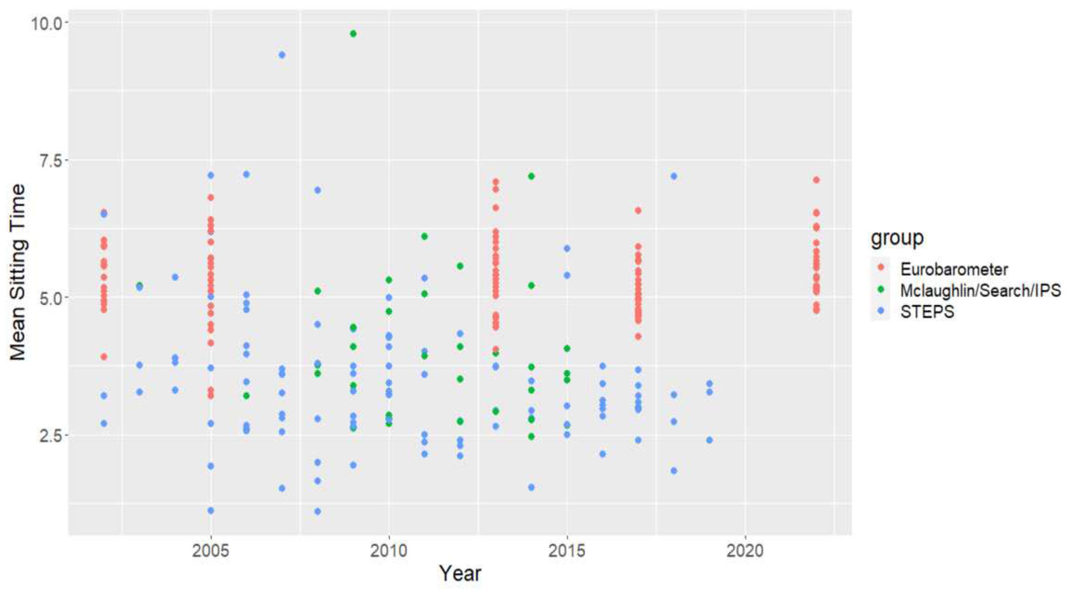
Table 1.
Factorial calculations of total energy expenditure for a population group (FAO/WHO/UNU 2001).
Table 1.
Factorial calculations of total energy expenditure for a population group (FAO/WHO/UNU 2001).
| Main daily activities Sedentary or light activity lifestyle |
Time allocation hours |
Energy cost PAR |
Time × energy cost | Mean PAL multiple of 24-hour BMR |
|---|---|---|---|---|
| Sleeping | 8 | 1 | 8.0 | |
| Personal care (dressing, showering) | 1 | 2.3 | 2.3 | |
| Eating | 1 | 1.5 | 1.5 | |
| Cooking | 1 | 2.1 | 2.1 | |
| Sitting (office work, selling produce, tending shop) | 8 | 1.5 | 12.0 | |
| General household work | 1 | 2.8 | 2.8 | |
| Driving car to/from work | 1 | 2.0 | 2.0 | |
| Walking at varying paces without a load | 1 | 3.2 | 3.2 | |
| Light leisure activities (watching TV, chatting) | 2 | 1.4 | 2.8 | |
| Total | 24 | 36.7 | 36.7/24 = 1.53 |
Table 2.
Data sources and definitions for variables.
| Variable | Source(s) | Mean | Standard Deviation | Min | Max |
|---|---|---|---|---|---|
| Mean Sitting Time (hours/day) | WHO STEPS, Eurobarometer surveys, Rezende et al., Mclaughlin et al. | 4.38 | 1.32 | 1.09 | 7.23 |
| Sample Standard Deviation of Sitting Time (hours/day) | WHO STEPS, Eurobarometer surveys, Rezende et al., Mclaughlin et al. | 3.19 | 1.99 | 0.32 | 21.20 |
| GDP Per Capita in 2015 USD | World Bank World Development Indicators | 19375.70 | 21110.30 | 334.73 | 107792.19 |
| Cellphone Subscriptions Per 100 Population | World Bank World Development Indicators | 88.40 | 42.76 | 0.09 | 205.91 |
| Proportion of Population Using the Internet | World Bank World Development Indicators | 45.10 | 32.09 | 0.22 | 98.87 |
| Upper Secondary Education Completion Rate | UNESCO | 0.64 | 0.30 | 0.02 | 0.98 |
| Rural Population Percentage | World Bank World Development Indicators | 39.60 | 22.77 | 0.00 | 84.57 |
| Percentage of Labor Employed in Agriculture, Forestry, and Fishing | FAOSTAT | 21.16 | 22.91 | 0.60 | 82.00 |
| Theil Index | World Bank Poverty and Inequality Platform | 0.21 | 0.09 | 0.07 | 0.63 |
| Population | World Bank Health Nutrition and Population Statistics | 24720068 | 85870996 | 1208 | 1337705000 |
Disclaimer/Publisher’s Note: The statements, opinions and data contained in all publications are solely those of the individual author(s) and contributor(s) and not of MDPI and/or the editor(s). MDPI and/or the editor(s) disclaim responsibility for any injury to people or property resulting from any ideas, methods, instructions or products referred to in the content. |
© 2023 by the authors. Licensee MDPI, Basel, Switzerland. This article is an open access article distributed under the terms and conditions of the Creative Commons Attribution (CC BY) license (http://creativecommons.org/licenses/by/4.0/).
Copyright: This open access article is published under a Creative Commons CC BY 4.0 license, which permit the free download, distribution, and reuse, provided that the author and preprint are cited in any reuse.


