Submitted:
21 November 2023
Posted:
22 November 2023
Read the latest preprint version here
Abstract
Keywords:
1. Introduction
2. Evaluating the Evolution of Efforts to Contest the Law of Energy Conservation
2.1. Scientific Perspective
2.2. Philosophical Perspective
2.3. Historical and Modern Shifts
2.4. The Need for a New Approach
3. Breaking the Law of Energy Conservation
3.1. The Energy Circuit-Unleashing the Power of Electrical Short Circuits
3.2. Design of the Proposed Energy Circuit (The Main Energy Circuit Operational Units)
- is the diode current.
- is the reverse saturation current.
- is the voltage across the diode.
- is the ideality factor (typically around for ideal diodes).
- is the thermal voltage, approximately at room temperature.
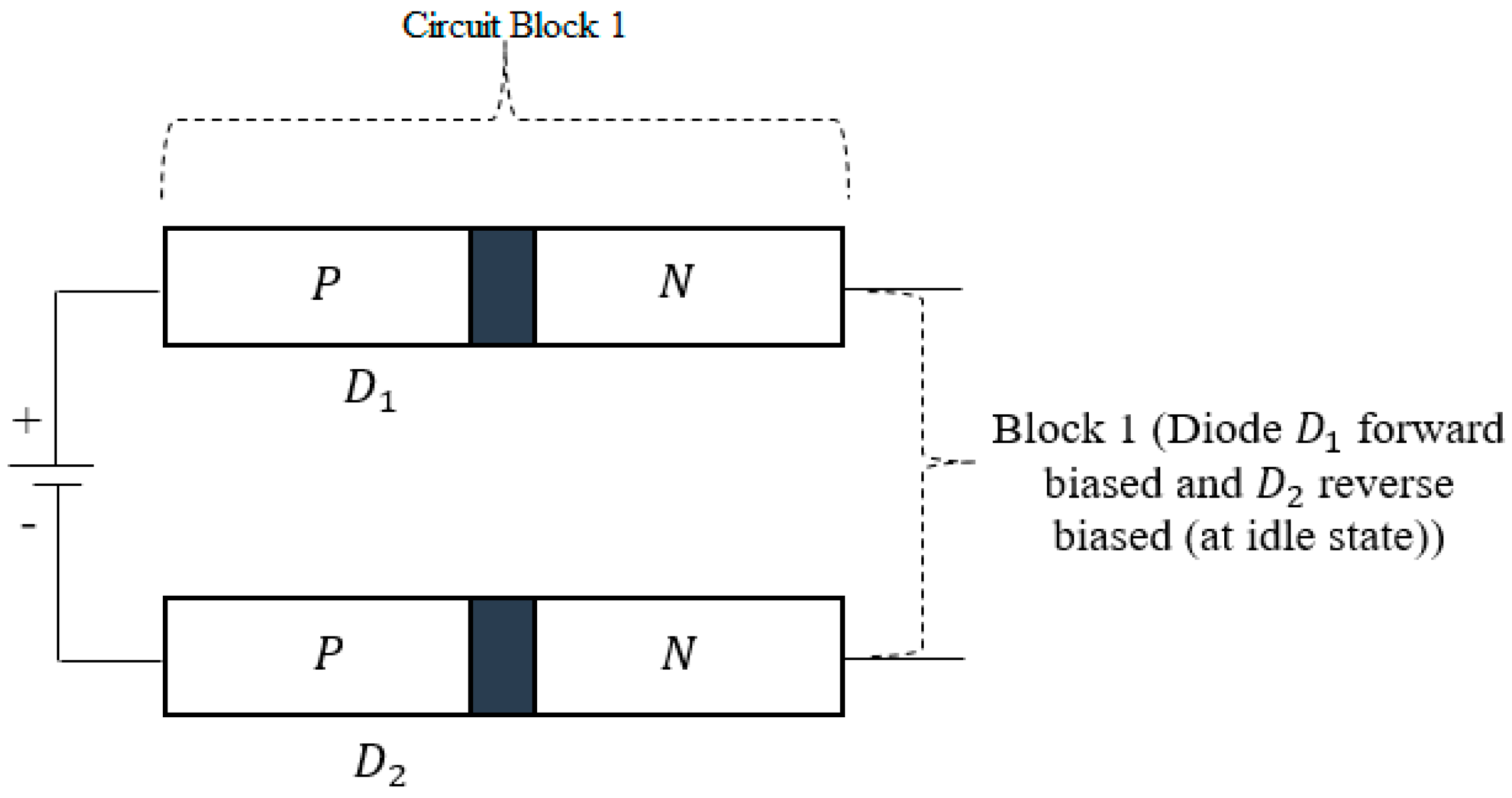
3.2.1. Operation Principles of Circuit Block 1 (Establishing Higher Resistive Circuit Element)
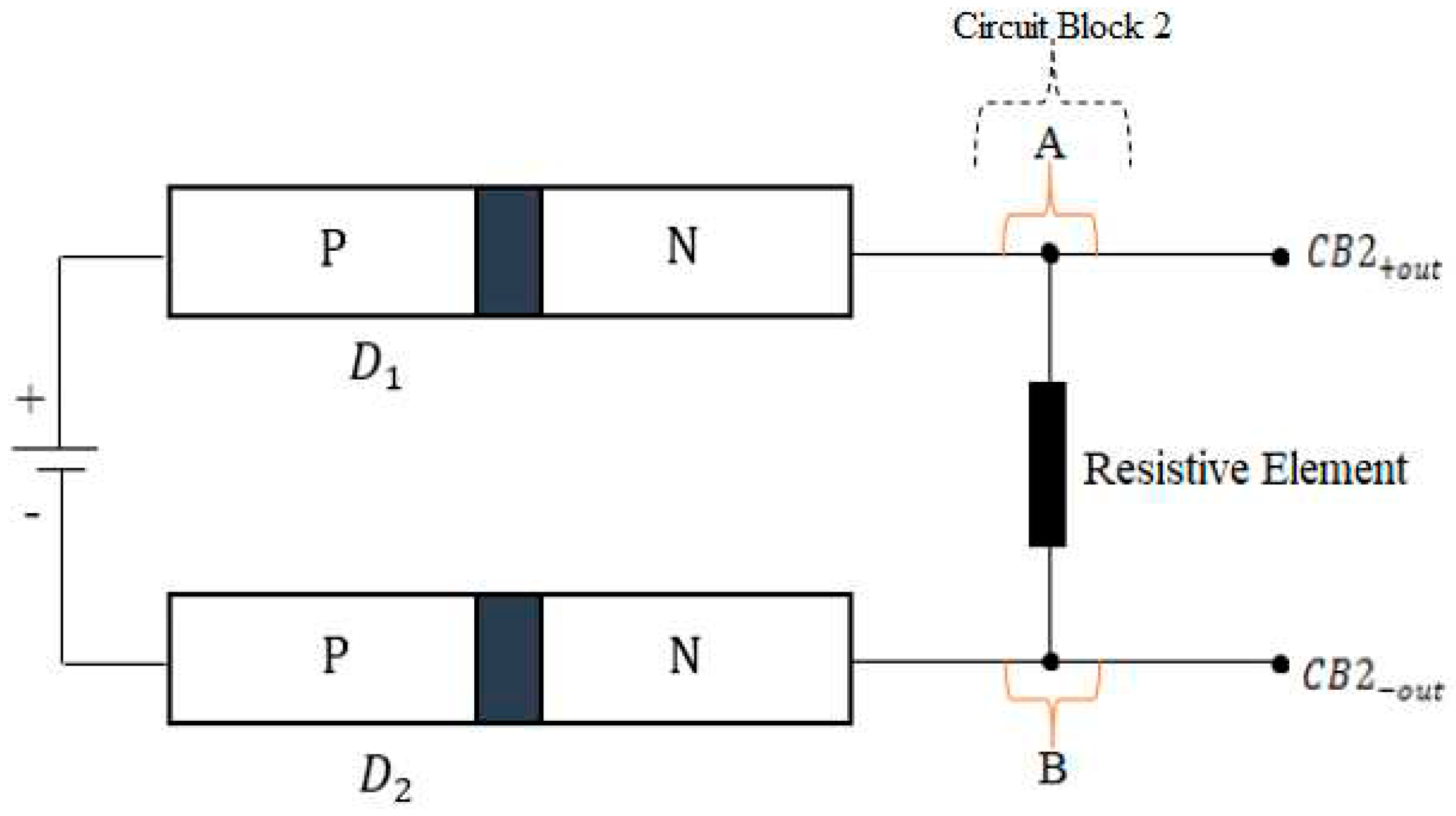
3.2.2. Description of Circuit Block 2 Components
3.2.3. Load Component_CB3 (Constant Current Boost Converter) Major Elements
- is the inductor value.
- is the desired output voltage.
- is the input voltage.
- is the duty cycle of the converter.
- is the switching frequency.
- is the peak-to-peak inductor ripple current.
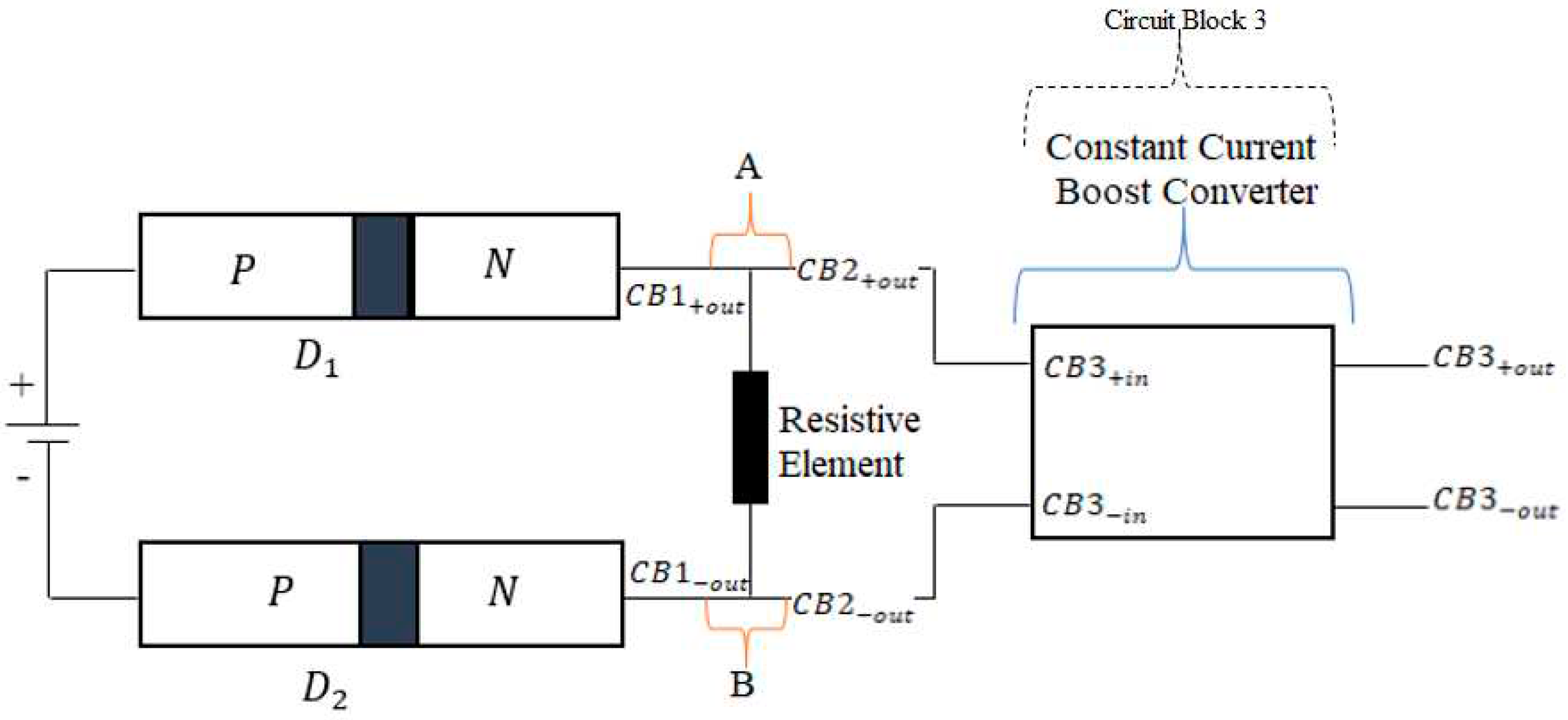
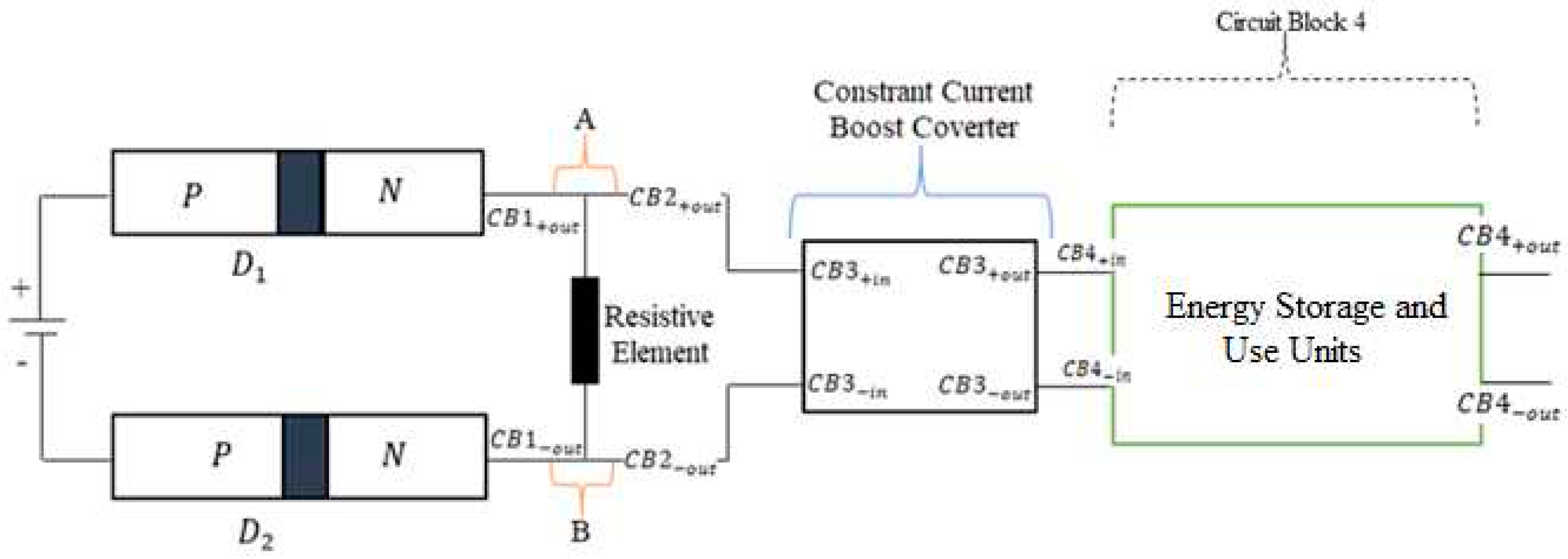
3.2.4. The Choice for Circuit Block 4 Unit
3.2.5. Design and Operation of the Sensing Element in Circuit Block 5
3.2.6. The Sensing Element Operation Mechanism
3.3. Overall Energy Circuit Representation
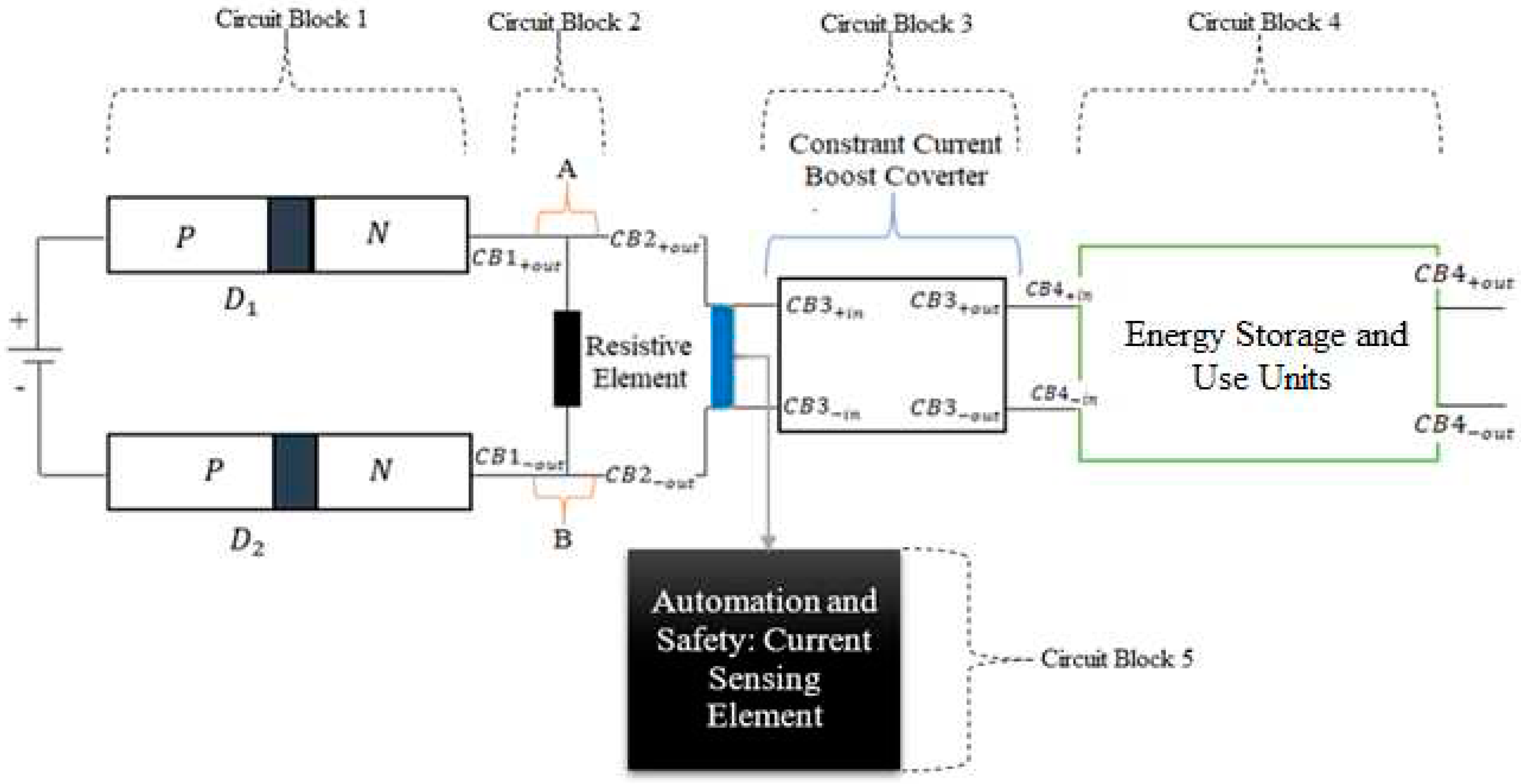
3.4. Interpretation and Simulation of the Proposed Energy Circuit Blocks
3.4.1. Simulated Results and Analysis
3.4.2. Description of Main Sections of the Simulation
3.4.3. Analysis of Simulation Results
3.4.4. Power Output from Circuit Block 3
3.5. Breaking the Law of Energy Conservation
3.6. Applications of the Energy Circuit-Addressing Some Critical Challenges
3.6.1. Energy Creation and Conservation
3.6.2. Applications in Electric Vehicles (EVs)
3.6.3. Microgrid Development
3.6.4. Renewable Energy Integration
3.6.5. Addressing the Energy Crisis
4. Discussion and Implications
4.1. Breaking Misconceptions and Limitations in Energy Conservation
4.2. Contributions to Addressing the Global Energy Crisis
4.3. Solutions to Noise Pollution and Innovations in Electric Vehicles
4.4. On Greenhouse Gas Reduction and Limitations of Current Clean Energy Systems
4.5. Innovations in Electronic Materials and Semiconductor Development
4.6. Challenging Philosophical Assumptions and Scientific Thinking
4.7. Merits over Current Systems-A Paradigm Shift in Energy Conservation
5. Conclusions
Author Contributions
Funding
Data Availability Statement
Conflicts of Interest
Appendix A Energy Circuit Simulation and Interpretation
Appendix B. The Modified Ohm’s Law and Its Application in Breaking the Law of Energy Conservation (Reflecting Real-World Scenarios)
- is the short circuit effect current.
- is the current scaling factor.
- is the resistance change due to the short circuit.
- is the reference resistance.
References
- P. Bradu et al., “Recent advances in green technology and Industrial Revolution 4.0 for a sustainable future,” Environ. Sci. Pollut. Res., Apr. 2022, . [CrossRef]
- M. Farghali et al., “Strategies to save energy in the context of the energy crisis: a review,” Environ. Chem. Lett., vol. 21, no. 4, pp. 2003–2039, Aug. 2023, . [CrossRef]
- Y. Guan et al., “Burden of the global energy price crisis on households,” Nat. Energy, vol. 8, no. 3, Art. no. 3, Mar. 2023, . [CrossRef]
- Gupta and O. Gupta, “Recent Advancements in the Recovery and Reuse of Organic Solvents Using Novel Nanomaterial-Based Membranes for Renewable Energy Applications,” Membranes, vol. 13, no. 1, p. 108, Jan. 2023, . [CrossRef]
- J. L. Holechek, H. M. E. Geli, M. N. Sawalhah, and R. Valdez, “A Global Assessment: Can Renewable Energy Replace Fossil Fuels by 2050?,” Sustainability, vol. 14, no. 8, Art. no. 8, Jan. 2022, . [CrossRef]
- G. Liobikienė, Y. Matiiuk, and R. Krikštolaitis, “The concern about main crises such as the Covid-19 pandemic, the war in Ukraine, and climate change’s impact on energy-saving behavior,” Energy Policy, vol. 180, p. 113678, Sep. 2023, . [CrossRef]
- S. Singh and J. Ru, “Accessibility, affordability, and efficiency of clean energy: a review and research agenda,” Environ. Sci. Pollut. Res., vol. 29, no. 13, pp. 18333–18347, Mar. 2022, . [CrossRef]
- J. Woodcock, D. Banister, P. Edwards, A. M. Prentice, and I. Roberts, “Energy and transport,” Lancet Lond. Engl., vol. 370, no. 9592, pp. 1078–1088, Sep. 2007, . [CrossRef]
- S. S. Akadiri, T. S. Adebayo, M. Nakorji, W. Mwakapwa, E. M. Inusa, and O.-O. Izuchukwu, “Impacts of globalization and energy consumption on environmental degradation: what is the way forward to achieving environmental sustainability targets in Nigeria?,” Environ. Sci. Pollut. Res. Int., vol. 29, no. 40, pp. 60426–60439, 2022, . [CrossRef]
- M. J. B. Kabeyi and O. A. Olanrewaju, “Sustainable Energy Transition for Renewable and Low Carbon Grid Electricity Generation and Supply,” Front. Energy Res., vol. 9, 2022, Accessed: Nov. 15, 2023. [Online]. Available: https://www.frontiersin.org/articles/10.3389/fenrg.2021.743114.
- N. Coppedge, “TOP PERPETUAL MOTION MACHINES,” May 2022.
- P. David, ELECTRO-MAGNETIC INDUCTION: FREE ELECTRICITY GENERATOR. 2017.
- S. P. C. Mohammad Noor Hidayat, “Design and Analysis of A Perpetual Motion Machine Using Neodymium Magnets as A Prime Mover,” J. Southwest Jiaotong Univ., vol. 56, no. 2, Art. no. 2, May 2021, Accessed: Nov. 15, 2023. [Online]. Available: http://jsju.org/index.php/journal/article/view/844.
- S. Khatri, “Design and analysis of Free Energy Generator system by balancing of flywheel,” Turk. Online J. Qual. Inq., vol. 13, no. 1, Art. no. 1, Jan. 2022, Accessed: Nov. 15, 2023. [Online]. Available: https://www.tojqi.net/index.php/journal/article/view/8694.
- J. F. Rodríguez-León, I. Cervantes, E. Castillo-Castañeda, G. Carbone, and D. Cafolla, “Design and Preliminary Testing of a Magnetic Spring as an Energy-Storing System for Reduced Power Consumption of a Humanoid Arm,” Actuators, vol. 10, no. 6, Art. no. 6, Jun. 2021, . [CrossRef]
- Satellite Research & Development Center/SUPARCO, Lahore 54000, Pakistan, I. Khan, M. Amin, M. I. Masood, and A. Asadullah, “Analysis of ‘free energy’ perpetual motion machine system based on permanent magnets,” Int. J. Smart Grid Clean Energy, 2014, . [CrossRef]
- B. Mahesh, “Self Flowing Generator,” Int. J. Sci. Res. IJSR, vol. 7, pp. 259–261, Apr. 2018, . [CrossRef]
- E. Mach, “On the Principle of the Conservation of Energy,” The Monist, vol. 5, no. 1, pp. 22–54, 1894, Accessed: Nov. 15, 2023. [Online]. Available: https://www.jstor.org/stable/27897203.
- P. Innocenzi, “Perpetuum Mobile,” in The Innovators Behind Leonardo, Cham: Springer International Publishing, 2019, pp. 165–180. [CrossRef]
- M. Davis, “No Perpetual Motion Machine,” Science, vol. 268, p. 624, May 1995, . [CrossRef]
- School Adviser of Natural Science Teachers of Ioannina8 Seferi street, Eleoussa, 455 00,Ioannina Hellas and D. Tsaousis, “Perpetual Motion Machine,” J. Eng. Sci. Technol. Rev., vol. 1, no. 1, pp. 53–57, Jun. 2008, . [CrossRef]
- J. Wisniak, “Conservation of Energy Readings on the Origins of the First Law of Thermodynamics. Part II,” Educ. Quím., vol. 19, no. 3, p. 216, Jun. 2011, . [CrossRef]
- M. N. Hidayat, S. P. Chairandy, and F. Ronilaya, “Design and Analysis of A Perpetual Motion Machine Using Neodymium Magnets as A Prime Mover,” J. Southwest Jiaotong Univ., vol. 56, no. 2, pp. 211–219, Apr. 2021, . [CrossRef]
- S. V. Kukhlevsky, “Breaking of Energy Conservation Law: Creating and Destroying of Energy by Subwavelength Nanosystems.” arXiv, Dec. 27, 2006. [CrossRef]
- S. Abdollahi, “Hypothesis of Nothingness,” vol. 10, pp. 43–49, Jul. 2021, . [CrossRef]
- B. N. Shanta, “Life and consciousness - The Vedāntic view,” Commun. Integr. Biol., vol. 8, no. 5, p. e1085138, 2015, . [CrossRef]
- S. Paulson, D. Albert, J. Holt, and N. Turok, “The origins of the universe: why is there something rather than nothing?,” Ann. N. Y. Acad. Sci., vol. 1361, pp. 1–17, Dec. 2015, . [CrossRef]
- S. Carroll, “Why Is There Something, Rather Than Nothing?,” Feb. 2018.
- T. R. Mongan, “Origin of the Universe, Dark Energy, and Dark Matter,” J. Mod. Phys., vol. 9, no. 5, Art. no. 5, Apr. 2018, . [CrossRef]
- M. Lincoln and A. Wasser, “Spontaneous creation of the Universe Ex Nihilo,” Phys. Dark Universe, vol. 2, no. 4, pp. 195–199, Dec. 2013, . [CrossRef]
- P. Heering, J. Keck, and G. A. Rohlfs, “Laboratory Notes, Laboratory Experiences, and Conceptual Analysis: Understanding the Making of Ohm’s First Law in Electricity,” Berichte Zur Wiss., vol. 43, no. 1, pp. 7–27, Mar. 2020, . [CrossRef]
- K. M. Tenny and M. Keenaghan, “Ohms Law,” in StatPearls, Treasure Island (FL): StatPearls Publishing, 2023. Accessed: Nov. 15, 2023. [Online]. Available: http://www.ncbi.nlm.nih.gov/books/NBK441875/.
- Rangel-Abundis, “[Shunt and short circuit],” Cir. Cir., vol. 74, no. 1, pp. 69–70, 2006.
- D. H. Chen, “Can Law of Conservation of Energy Be Broken?,” Appl. Mech. Mater., vol. 192, pp. 420–424, Jul. 2012, . [CrossRef]
- T. Kerremans, P. Samuelsson, and P. P. Potts, “Probabilistically Violating the First Law of Thermodynamics in a Quantum Heat Engine,” SciPost Phys., vol. 12, no. 5, p. 168, May 2022, . [CrossRef]
- J. V. N., “Particle Creation in a Big-bang Universe,” Nature, vol. 246, no. 5433, Art. no. 5433, Dec. 1973, . [CrossRef]
- R. L. Anjum and S. Mumford, “A Powerful Theory of Causation,” vol. 9780203851289, Jan. 2010, . [CrossRef]
- Kimuya, Proving the Law of Energy Conservation from Mathematical and Scientific Perspectives. 2022. [CrossRef]
- H. Lee, W. Chow, and H. Hung, “A Study on Residential Fires due to Electrical Faults in Hong Kong,” 2016. Accessed: Nov. 15, 2023. [Online]. Available: https://www.semanticscholar.org/paper/A-Study-on-Residential-Fires-due-to-Electrical-in-Lee-Chow/05000136e6f2ca0a48bc05b63af08265a218ab7c.
- H. Lee, W. Chow, and H. Hung, “A Study on Residential Fires due to Electrical Faults in Hong Kong,” 2016. Accessed: Nov. 15, 2023. [Online]. Available: https://www.semanticscholar.org/paper/A-Study-on-Residential-Fires-due-to-Electrical-in-Lee-Chow/05000136e6f2ca0a48bc05b63af08265a218ab7c.
- J.-H. Kim, B.-K. Park, J.-H. Song, and K.-C. Jung, “A Study on the Possibility of Electrical Fires due to the Short Circuit and Ground Fault of Power Cable Supported by an Iron Fence,” J. Korean Soc. Saf., vol. 22, Jan. 2007.
- 2022; G. Buica, A. Anca Elena, C. Beiu, M. Risteiu, and D. Pasculescu, “Aspects of the earthing and short-circuit device’s safety quality,” MATEC Web Conf., vol. 373, Dec. 2022, . [CrossRef]
- L. Salvaraji, M. S. Jeffree, K. Awang Lukman, S. Saupin, and R. Avoi, “Electrical safety in a hospital setting: A narrative review,” Ann. Med. Surg., vol. 78, p. 103781, May 2022, . [CrossRef]
- S. Szultka, S. Czapp, A. Tomaszewski, and H. Ullah, “Evaluation of Fire Hazard in Electrical Installations Due to Unfavorable Ambient Thermal Conditions,” Fire, vol. 6, no. 2, Art. no. 2, Feb. 2023, . [CrossRef]
- D. Gao and Q. Liu, “Review of the Research on the Identification of Electrical Fire Trace Evidence,” Procedia Eng., vol. 135, pp. 29–32, Dec. 2016, . [CrossRef]
- B. B. Pannebakker, A. C. de Waal, and W. G. J. H. M. van Sark, “Photovoltaics in the shade: one bypass diode per solar cell revisited,” Prog. Photovolt. Res. Appl., vol. 25, no. 10, pp. 836–849, 2017, . [CrossRef]
- F. Fadliondi, H. Isyanto, and B. Budiyanto, “Bypass Diodes for Improving Solar Panel Performance,” Int. J. Electr. Comput. Eng. IJECE, vol. 8, p. 2703, Oct. 2018, . [CrossRef]
- M. Sofyan, I. Sara, and S. Suriadi, The effect of bypass diode installation on partially covered solar panel output power, vol. 1087. 2021. [CrossRef]
- J. H. Lee et al., “Characteristics and Electronic Band Alignment of a Transparent p-CuI/n-SiZnSnO Heterojunction Diode with a High Rectification Ratio,” Nanomaterials, vol. 11, no. 5, Art. no. 5, May 2021, . [CrossRef]
- C. SHARMA, “Solar Panel Mathematical Modeling Using Simulink,” Int. J. Eng. Res. Appl., vol. 4, pp. 67–72, May 2014.
- Z. Chen, R. Xiong, J. Tian, X. Shang, and J. Lu, “Model-based fault diagnosis approach on external short circuit of lithium-ion battery used in electric vehicles,” Appl. Energy, vol. 184, pp. 365–374, Dec. 2016, . [CrossRef]
- B. Xia, Z. Chen, C. Mi, and B. Robert, “External short circuit fault diagnosis for lithium-ion batteries,” in 2014 IEEE Transportation Electrification Conference and Expo (ITEC), Dearborn, MI: IEEE, Jun. 2014, pp. 1–7. [CrossRef]
- KIMUYA, A. M. The Modified Ohm’s Law and Its Implications for Electrical Circuit Analysis. Eurasian J. Sci. Eng. Tech. 2023, 4(2), Accepted for publication: 10.11.2023.
- F. A. Chaves, P. C. Feijoo, and D. Jiménez, “2D pn junctions driven out-of-equilibrium,” Nanoscale Adv., vol. 2, no. 8, p. 3252, Aug. 2020, . [CrossRef]
- S. K. Tripathi and M. Sharma, “Analysis of the forward and reverse bias I-V and C-V characteristics on Al/PVA:n-PbSe polymer nanocomposites Schottky diode,” J. Appl. Phys., vol. 111, no. 7, p. 074513, Apr. 2012, . [CrossRef]
- J. R. Sadaf, M. Q. Israr, S. Kishwar, O. Nur, and M. Willander, “Forward- and reverse-biased electroluminescence behavior of chemically fabricated ZnO nanotubes/GaN interface,” Semicond. Sci. Technol., vol. 26, no. 7, p. 075003, Jul. 2011, . [CrossRef]
- X. Zhang et al., “Near-ideal van der Waals rectifiers based on all-two-dimensional Schottky junctions,” Nat. Commun., vol. 12, p. 1522, Mar. 2021, . [CrossRef]
- Z. Botao, W. Qi, Z. Min, and H. Huan, “Analytical solution for the inductor current of BOOST converter,” IET Power Electron., vol. 12, no. 9, pp. 2424–2432, 2019, . [CrossRef]
- Z. Li et al., “Aqueous hybrid electrochemical capacitors with ultra-high energy density approaching for thousand-volts alternating current line filtering,” Nat. Commun., vol. 13, p. 6359, Oct. 2022, . [CrossRef]
- P. Xia, Z. Zhang, Z. Tang, Y. Xue, J. Li, and G. Yang, “Preparation and Electrochemical Performance of Three-Dimensional Vertically Aligned Graphene by Unidirectional Freezing Method,” Molecules, vol. 27, no. 2, p. 376, Jan. 2022, . [CrossRef]
- Y. Yuan, C. Wang, K. Lei, H. Li, F. Li, and J. Chen, “Sodium-Ion Hybrid Capacitor of High Power and Energy Density,” ACS Cent. Sci., vol. 4, no. 9, pp. 1261–1265, Sep. 2018, . [CrossRef]
- N. Kumar, S.-B. Kim, S.-Y. Lee, and S.-J. Park, “Recent Advanced Supercapacitor: A Review of Storage Mechanisms, Electrode Materials, Modification, and Perspectives,” Nanomaterials, vol. 12, no. 20, p. 3708, Oct. 2022, . [CrossRef]
- Q. Zhu, J. Ma, S. Li, and D. Mao, “Solid-State Electrolyte for Lithium-Air Batteries: A Review,” Polymers, vol. 15, no. 11, p. 2469, May 2023, . [CrossRef]
- P. Lai et al., “Bifunctional Localized High-Concentration Electrolyte for the Fast Kinetics of Lithium Batteries at Low Temperatures,” ACS Appl. Mater. Interfaces, vol. 15, no. 25, pp. 31020–31031, Jun. 2023, . [CrossRef]
- J. M. Lim et al., “Advances in high-voltage supercapacitors for energy storage systems: materials and electrolyte tailoring to implementation,” Nanoscale Adv., vol. 5, no. 3, pp. 615–626, . [CrossRef]
- P. Yang et al., “Ultrafast-Charging Supercapacitors Based on Corn-Like Titanium Nitride Nanostructures,” Adv. Sci., vol. 3, no. 6, p. 1500299, Oct. 2015, . [CrossRef]
- Y. Xu et al., “High Performance Supercapacitors Based on Mesopore Structured Multiwalled Carbon Nanotubes,” ChemistryOpen, vol. 10, no. 3, pp. 347–351, Feb. 2021, . [CrossRef]
- Tomczewski, “Operation of a wind turbine-flywheel energy storage system under conditions of stochastic change of wind energy,” ScientificWorldJournal, vol. 2014, p. 643769, 2014, . [CrossRef]
- S. Wicki and E. G. Hansen, “Clean energy storage technology in the making: An innovation systems perspective on flywheel energy storage,” J. Clean. Prod., vol. 162, pp. 1118–1134, Sep. 2017, . [CrossRef]
- Mardani, A. Jusoh, E. Zavadskas, F. Cavallaro, and Z. Khalifah, “Sustainable and Renewable Energy: An Overview of the Application of Multiple Criteria Decision Making Techniques and Approaches,” Sustainability, vol. 7, no. 10, pp. 13947–13984, Oct. 2015, . [CrossRef]
- Zohuri and P. McDaniel, “First Law of Thermodynamics,” in Thermodynamics in Nuclear Power Plant Systems, Cham: Springer International Publishing, 2019, pp. 99–148. [CrossRef]
- Kutty, R. Al-Jondob, G. Abdella, and T. El-Mekkawy, A Frontier Based Eco-Efficiency Assessment of Electric Vehicles: The Case of European Union Countries Using Mixed and Renewable Sources of Energy. 2021.
- Costa, J. Barbosa, H. Castro, R. Gonçalves, and S. Lanceros-Méndez, “Electric vehicles: To what extent are environmentally friendly and cost effective? – Comparative study by european countries,” Renew. Sustain. Energy Rev., vol. 151, p. 111548, Nov. 2021, . [CrossRef]
- J. A. Sanguesa, V. Torres-Sanz, P. Garrido, F. J. Martinez, and J. M. Marquez-Barja, “A Review on Electric Vehicles: Technologies and Challenges,” Smart Cities, vol. 4, no. 1, pp. 372–404, Mar. 2021, . [CrossRef]
- Sbordone, I. Bertini, B. Di Pietra, M. C. Falvo, A. Genovese, and L. Martirano, “EV fast charging stations and energy storage technologies: A real implementation in the smart micro grid paradigm,” Electr. Power Syst. Res., vol. 120, pp. 96–108, Mar. 2015, . [CrossRef]
- V. Rajendran Pillai, R. Rajasekharan Nair Valsala, V. Raj, M. Petra, S. Krishnan Nair, and S. Mathew, “Exploring the Potential of Microgrids in the Effective Utilisation of Renewable Energy: A Comprehensive Analysis of Evolving Themes and Future Priorities Using Main Path Analysis,” Designs, vol. 7, no. 3, p. 58, Apr. 2023, . [CrossRef]
- Hirsch, Y. Parag, and J. Guerrero, “Microgrids: A review of technologies, key drivers, and outstanding issues,” Renew. Sustain. Energy Rev., vol. 90, pp. 402–411, Jul. 2018, . [CrossRef]
- M. Uddin, H. Mo, D. Dong, S. Elsawah, J. Zhu, and J. M. Guerrero, “Microgrids: A review, outstanding issues and future trends,” Energy Strategy Rev., vol. 49, p. 101127, Sep. 2023, . [CrossRef]
- M. R. H. Mojumder, F. Ahmed Antara, M. Hasanuzzaman, B. Alamri, and M. Alsharef, “Electric Vehicle-to-Grid (V2G) Technologies: Impact on the Power Grid and Battery,” Sustainability, vol. 14, no. 21, Art. no. 21, Jan. 2022, . [CrossRef]
- M. Farghali et al., “Social, environmental, and economic consequences of integrating renewable energies in the electricity sector: a review,” Environ. Chem. Lett., vol. 21, no. 3, pp. 1381–1418, Jun. 2023, . [CrossRef]
- M. Takase, R. Kipkoech, and P. K. Essandoh, “A comprehensive review of energy scenario and sustainable energy in Kenya,” Fuel Commun., vol. 7, p. 100015, Jun. 2021, . [CrossRef]
| Supply Voltage (V) | R0 (Ohms) | Ideality Factor (n) | Saturation Current () (A) | (W) | (A) | (W) | (W) |
Disclaimer/Publisher’s Note: The statements, opinions and data contained in all publications are solely those of the individual author(s) and contributor(s) and not of MDPI and/or the editor(s). MDPI and/or the editor(s) disclaim responsibility for any injury to people or property resulting from any ideas, methods, instructions or products referred to in the content. |
© 2023 by the authors. Licensee MDPI, Basel, Switzerland. This article is an open access article distributed under the terms and conditions of the Creative Commons Attribution (CC BY) license (http://creativecommons.org/licenses/by/4.0/).


