Preprint
Article

Dual Theory of Decaying Turbulence. 2. Numerical Simulation and Continuum Limit

This version is not peer-reviewed.

Submitted:

19 December 2023

Posted:

20 December 2023

Read the latest preprint version here

Abstract
This is the second paper in a cycle investigating the exact solution of loop equations in decaying turbulence. We perform numerical simulations of the Euler ensemble, suggested in the previous work, as a solution to the loop equations. We designed novel algorithms for simulation, which take a small amount of computer RAM so that only the CPU time grows linearly with the size of the system and its statistics. This algorithm allows us to simulate systems with billions of discontinuity points on our fractal curve, dual to the decaying turbulence. For the vorticity correlation function, we obtain quantum scaling laws with regime changes between effective indexes drifting with the logarithm of scale. The traditional description of turbulence with fractal or multifractal scaling laws does not apply here. In particular, the effective fractal dimension of our curve is a function of the scale. The measured conditional probabilities of fluctuating variables are smooth functions of the logarithm of scale, with statistical errors being negligible at our large number of random samples $T = 167,772,160$ with $N = 200,000,000$ points on a fractal curve. The quantum jumps arise from the analytical distribution of scaling variable $X = \frac{\cot^2(\pi p/q)}{q^2}$ where $\frac{p}{q}$ is a random fraction. This distribution is related to the totient summatory function and is a discontinuous function of $X$. In particular, the energy spectrum has quantum levels on top of a continuous background.
Keywords: 
Subject: 
Physical Sciences  -   Fluids and Plasmas Physics

1. Introduction

In 1993, we suggested [1] nonperturbative approach to Navier-Stokes turbulence based on the loop equations previously introduced in the gauge theory [2,3].
The Wilson loop average for the turbulence
Ψ [ γ , C ] = exp ı γ ν d θ C ( θ ) · v ( C ( θ ) ) i n i t
treated as a function of time and a functional of the periodic function C : r = C ( θ ) ; θ ( 0 , 2 π ) (not necessarily a single closed loop), satisfies certain functional equation which was defined and studied in these papers.
The averaging i n i t corresponds to averaging over an ensemble of solutions with different initial data. One does not need to specify this ensemble to obtain the Hopf or loop equation.
We are not going into details of the loop technology but shall investigate the solution found in the recent paper [4].

2. The theory

This solution has the following form
Ψ [ γ , C ] = exp ı γ ν d θ C ( θ ) · P ( θ ) F
The averaging F corresponds to averaging over an ensemble of solutions for F ( θ ) to be specified below.
This periodic vector function P ( θ ) also depends of time as follows
  P ( θ , t ) = ν 2 ( t + t 0 ) F ( θ ) γ ;     (4)
The time-independent function F ( θ ) satisfies two singular equations
( Δ F ) 2 = 1 ;
( 2 F · Δ F ı γ ) 2 + γ 2 = 4 F 2 ;
Δ F = F ( θ + 0 ) F ( θ 0 ) ;
F = F ( θ + 0 ) + F ( θ 0 ) 2 ;
This equation describes a fixed point regime of the loop equations for decaying turbulence. No approximations have been made so far.
This F ( θ ) is a fractal curve in complex 3D space, with discontinuity Δ F at every angle θ .
The solution in [4] builds such a curve as a limit of the polygon with N vertexes. The positions F k = F ( 2 π k / N ) of these vertices satisfy the recurrent equation
F k + 1 F k 2 = 1 ;
F k + 1 2 F k 2 ı γ 2 + γ 2 = F k + 1 + F k 2
There could be many solutions of such equations in d > 2 dimensions, as these are two complex equations relating d complex parameters in F k + 1 to those in F k .
Thus, there are d 2 complex parameters undetermined in every step q k = F k + 1 F k . This degeneration makes this a Markov chain or a random walk where each step depends only on a current position plus some arbitrary (random) parameters.

2.1. The Euler ensemble and its continuum limit

In particular, the following solution, found in [4], has some acceptable physical properties. We call it the Euler ensemble.
  F k = 1 2 csc β 2 Ω ^ · cos ( α k ) , sin ( α k ) w , i cos β 2 ;
Ω ^ O ( d ) ;
β = 2 π p q ;
0 < p < q < N ;
α k = β 0 k 1 σ l ;
σ k 2 = 1 ;
  0 N 1 σ l = q r ;
N q r N ;
( N r q ) ( mod 2 ) = 0 ;
Here p , q , r , N are positive integers, Ω ^ is a random rotation matrix in O ( d ) , and w S d 3 is a unit vector in d 2 dimensional space R d 2 .
This paper only considers the three-dimensional space d = 3 where w = ± 1 . This sign factor can be absorbed into a redefinition of σ l .
This sequence with arbitrary signs σ k = ± 1 subject to periodicity constraint (13) solves recurrent equation (6) independently of γ .
This ensemble consists of random p , q , r , N , σ 0 σ N 1 subject to periodicity conditions; we called it an Euler ensemble.
The ergodic hypothesis of [4] states that each element of the Euler ensemble enters with equal weight. This includes every set of σ l satisfying periodic boundary condition (13), every pair of coprime numbers 0 < p < q < N , gcd ( p , q ) = 1 and every q , r , N with ( N q r ) ( mod 2 ) = 0 .
The number theory counts these states using Euler totients.
A unique property of this solution is that the velocity circulation is real in this solution, as it should, despite the complex values of F k .
This cancellation of the imaginary part happens because of the closure (i.e., periodicity) of both loops C ( θ ) , F ( θ )
d θ C ( θ ) · F ( θ ) = d θ C ( θ ) · F ( θ ) ; ;
k Δ C k · F k = k C k · Δ F k ;
The discontinuity (i.e., the polygon side) is a real unit vector :
q k = Δ F k = σ k Ω ^ · { sin δ k , w cos δ k , 0 } ;
δ k = α k + β σ k 2 ;
The sum over all different configurations of the Euler ensemble with exponential weight exp μ N is called a grand canonical ensemble, using the language of statistical physics. The number theory counting using Euler totients [5] produces the following general formula [4]
Z ( μ ) = N Z ( N , N ) e μ N ;
F ( p , q , r , N ) E ( μ ) = N e μ N 2 < q < N p = 1 ( p , q ) = 1 q 1 r 2 | ( N q r ) F ( p , q , r , N ) Z ( μ ) ;
At the critical point μ 0 , the even N dominate, with the following result
Z ( μ ) 1 2 9 2 2 π 2 μ 5 / 2
The enstrophy, defined as an expectation value of the square of local vorticity, reduces in this theory to the following time-dependent formula [4]
  ω ( 0 ) 2 = 1 ( t + t 0 ) 2 2 N 4 S ( q ) N q 2 r 2 N ( N + q r ) / 2 E ( μ ) ;
S ( q ) = p = 1 ( p , q ) = 1 q 1 cot 2 π p q ;
We have found the method to compute this sum of squares of cotangent of all fractions of π with a given denominator analytically. This result was quoted in [4] and then generalized to arbitrary powers of cotangent.
This method is described in Appendix A

2.2. Small Euler ensemble at large N

At a fixed large value of q, the CDF of x = β / ( 2 π ) is given by the ratio of the Euler totient functions, asymptotically equal to x at large q
P ( β < 2 π x q ) = φ ( x q ) φ ( q ) x ;
The CDF of q is proportional to the totient summatory function
Φ ( n ) = k = 1 n φ ( k ) 6 π 2 n 2
Thus, the normalized CDF of y = q / N
P ( q < y N ) y 2 ;
f y ( y ) 2 y θ ( y ) θ ( 1 y ) ;
As we shall see, rather than β , we would need an asymptotic distribution of a scaling variable
X ( p , q ) = 1 q 2 cot 2 π p q 1 π 2 p 2
The β N variable can be related to y and X ( p , q )
β N = 2 N arcCot ( q X ) 2 y X ;
This distribution for X ( p , q ) at fixed q N can be found analytically, using newly established relations for the cotangent sums (see Appendix in [4]). Asymptotically, at large q these relations read
X n lim q 1 q p = 1 ( p , q ) q 1 X ( p , q ) n = δ n , 0 + 2 π 2 n ζ ( 2 n ) ( 2 n + 1 ) ζ ( 2 n + 1 )
This relation can be transformed further as
X n = 1 if n = 0 2 k = 1 φ ( k ) k ( 2 n + 1 ) ( 2 n + 1 ) π 2 n if n > 0
The Mellin transform of these moments leads to the following singular distribution
  X n = 0 W ( X ) d X X n ;
  W ( X ) = ( 1 α ) δ ( X 0 + ) + π Φ 1 π X ;
α = 0 π Φ 1 π X d X = π k = 1 φ ( k ) 2 k + 1 k 2 ( k + 1 ) 2 = 0.387153
where Φ ( n ) is the totient summatory function
The first term ( 1 α ) δ ( X 0 + ) accumulates the contribution from the vicinity of the finite lower limit of X
X m i n = X q / 2 1 , q π 2 q 4 = 0 +
This lower limit tends to zero, which leaves some part of the delta function out of the support of probability distribution. Normalizing the base moment X 0 = 1 yields the correction factor ( 1 α ) in front of the delta function. Therefore, the α part of the delta function in the normalized distribution falls below the lower limit, with the remaining part ( 1 α ) staying in the support of the distribution.
The upper limit of X
X m a x = X q 1 , q 1 π 2
Our distribution (33) is consistent with this upper limit, as the argument 1 π X becomes zero at X π 2 > 1 . It is plotted in Figure 1, except for the delta function part at infinitesimal X.
Once we are zooming into the tails of the p , q distribution, we also must recall that
P ( q < y N ) = Φ N y ;
  f y ( y ) = q = 2 δ y q N φ ( q )
The variable s also has a nontrivial distribution in the small Euler ensemble with even N , with a dominant contribution at s = 0 as conjectured in [4] and proven in [6]
f s ( s ) = δ ( s ) + O N 1 2

3. The big Euler ensemble as a Markov process

3.1. Numerical Simulations

We took N = 200 , 000 , 000 and generated T = 167 , 772 , 160 random data samples for β , ω n · ω m , S n , m S m , n with randomly chosen 0 n < m < N .
We devised a fast Python/CPP algorithm for this simulation, described in Appendix B. We ran it on an NYUAD cluster Jubail, which took about a week altogether, for three GPU runs and three CPU runs, which we all pooled into one dataset and binned by 2 20 intervals by the ranking of log cot 2 ( β / 2 ) . Two datasets were created, one for each sign of ω n · ω m .
We used a recursive rank-binning algorithm based on the standard library function nth element , which finds the median of unordered data by partial sorting in place in O ( N ) time. We recursively applied this function in parallel to each of the two halves of the array of data. The CPU time of this recursive parallel code is linear, as the geometric series N + N / 2 + N / 4 + adds up to 2 N .
Each interval contained only n = 80 ± 1 data points n , c ¯ , Δ c , s ¯ , Δ s , w ¯ , Δ w , where
c = 2 log cot ( β / 2 ) ;
s = log S n , m S m , n ;
w = log | ω n · ω m | ;
and x ¯ , Δ x denotes mean and standard deviation. Later, we used these data with Gaussian errors for the statistical analysis. We used logarithms because the values varied by several orders of magnitude, preventing statistical analysis.
The code was optimized to take O ( N 0 ) RAM, so the CPU and GPU resources of all 200 nodes were used to collect statistics. This optimization allows us to simulate astronomical ensembles of random fractions without hitting memory limits.
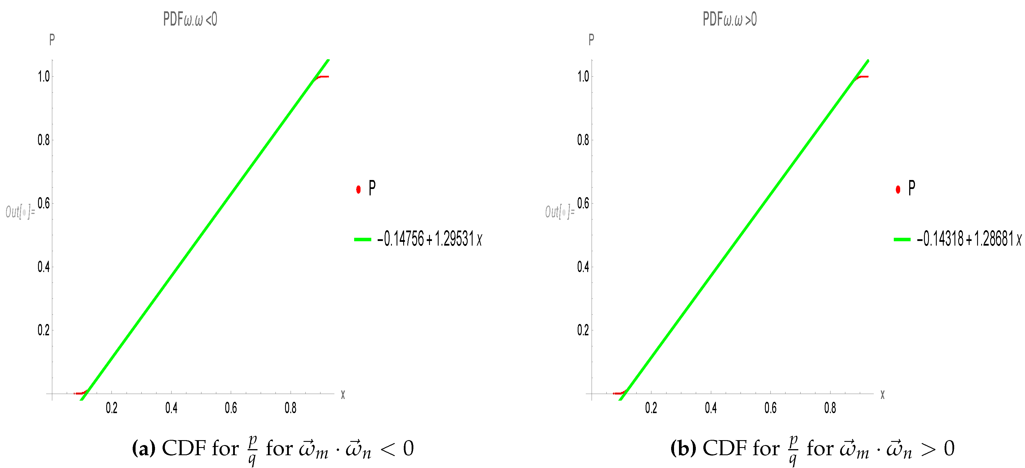
The first thing we measured was the distribution of x = β 2 π = p q , which we know in advance to be uniform except for small regions of x 1 / N , 1 x 1 / N , where quantization plays the role.
The measured distribution supports this hypothesis (see Figure 2).
The CDF is linear, supporting the uniform distribution of p q except for the endpoints ( 0 , 1 ) .
However, the critical phenomena in our system are related to these two endpoints where the scaling factor cot 2 ( β / 2 ) grows to q 2 . The uniform distribution of β corresponds to the variable X = q 2 cot 2 ( β / 2 ) distributed at large q as
f X ( X q ) q 1 X 3 2
The exact asymptotic distribution for the same variable has the form (34), found in the previous section.

3.2. Scaling variables in continuum limit

This quantum distribution is too complicated to reproduce in numerical simulation, but we measured distributions of other variables that behave smoother.
We studied the distribution of two variables involved in the correlation function (see next section)
D S = q 1 S n , m S m , n ;
W W = q 2 ω m · ω n ;
We multiplied both variables by powers of q to make them finite in the statistical limit q N .
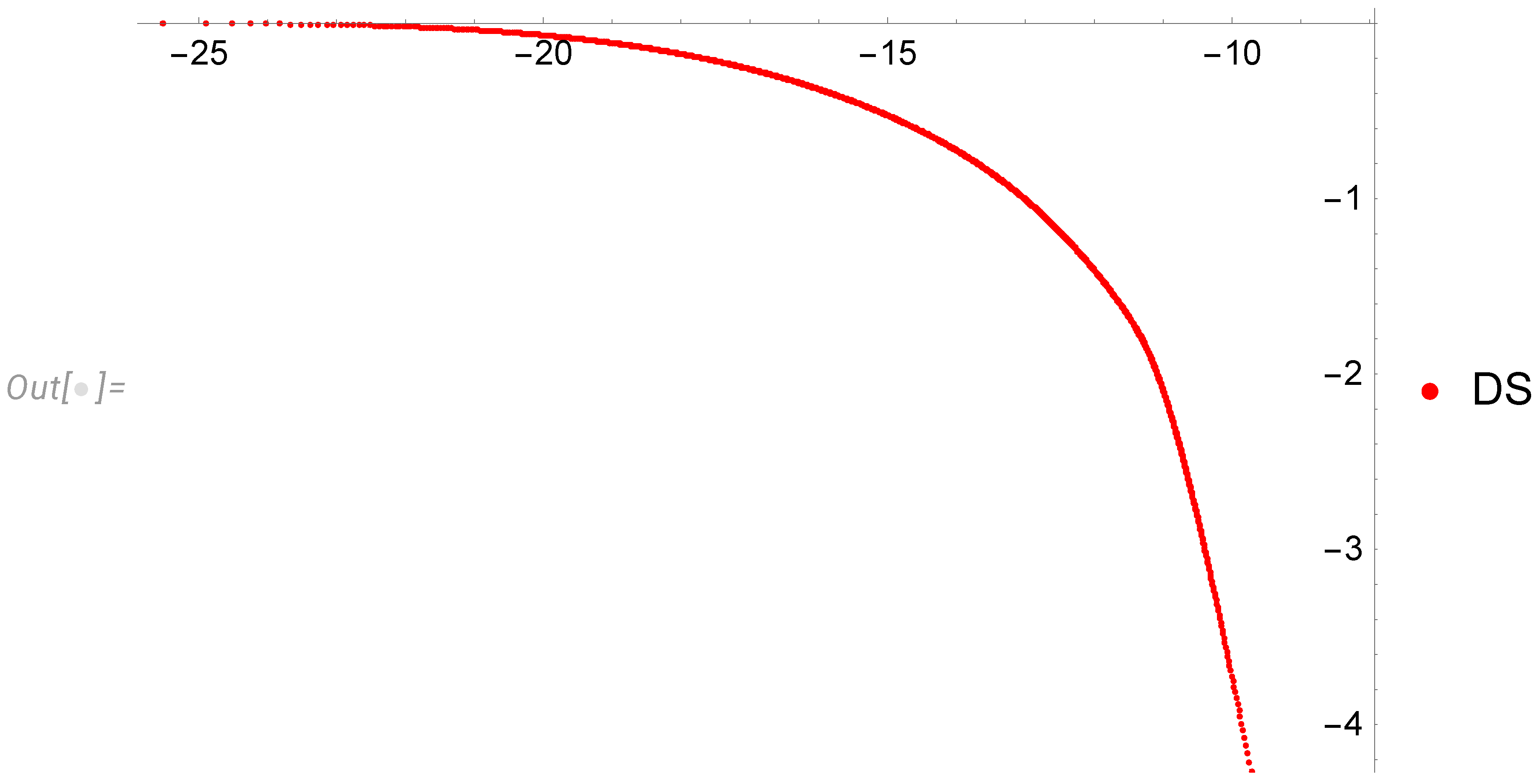
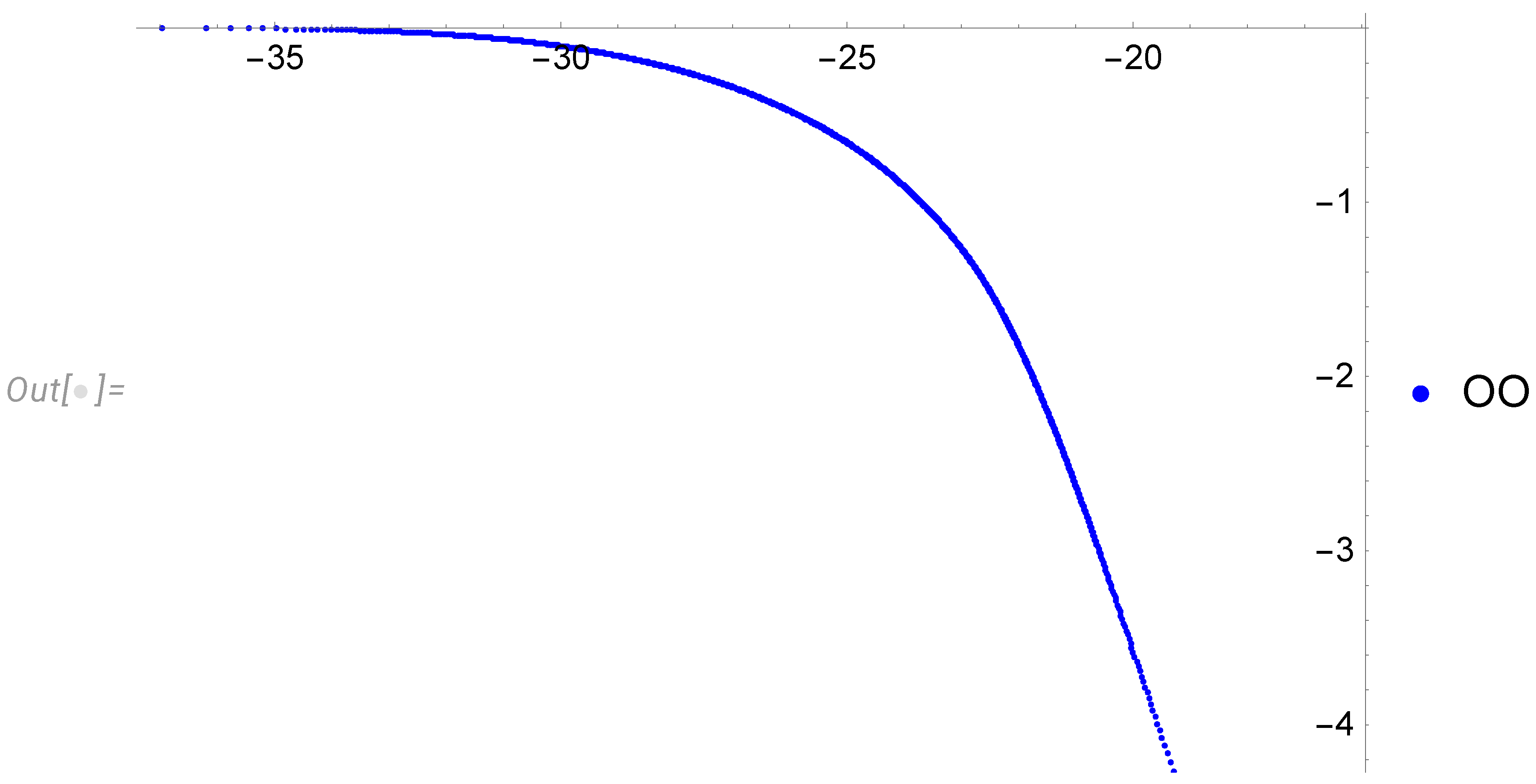
The distributions of these variables are shown in Figure 3 and Figure 4.
The variable D S measures the mean Euclidean distance between two random points on a curve in the embedding 3D complex space.
Let us study the moments of this distribution. Integrating by part in the standard definition, we have
( D S ) n = W ( D S ) ( D S ) n d ( D S ) = n ( 1 W ( D S ) ) ( D S ) n 1 d ( D S ) =
exp n ξ + T ( ξ ) + log n d ξ ;
T ( ξ ) = log ( 1 W exp ξ ;
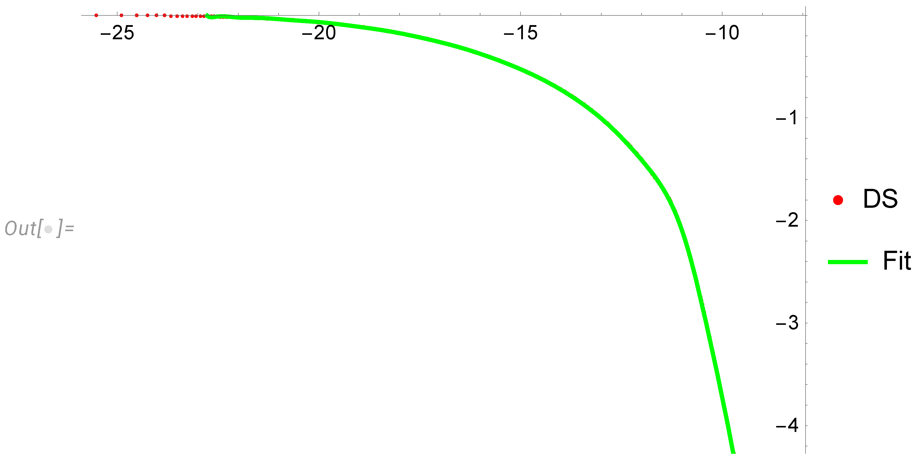
Our data was fit perfectly by 20 Chebyshev polynomials for this T ( ξ ) (see [7] and Figure 5).
The definition of effective index can be given as
η ( n ) = log ( D S ) n log D S ;
The saddle point computation of this integral gives the following parametric equations
n = T ( ξ ) ;
log ( D S ) n L n ( ξ ) = n ξ + T ( ξ ) + log n n = T ( ξ ) ;
L 1 = ξ 1 + T ( ξ 1 ) 1 = T ( ξ 1 ) ;
η ( T ( ξ ) ) = L n ( ξ ) L 1
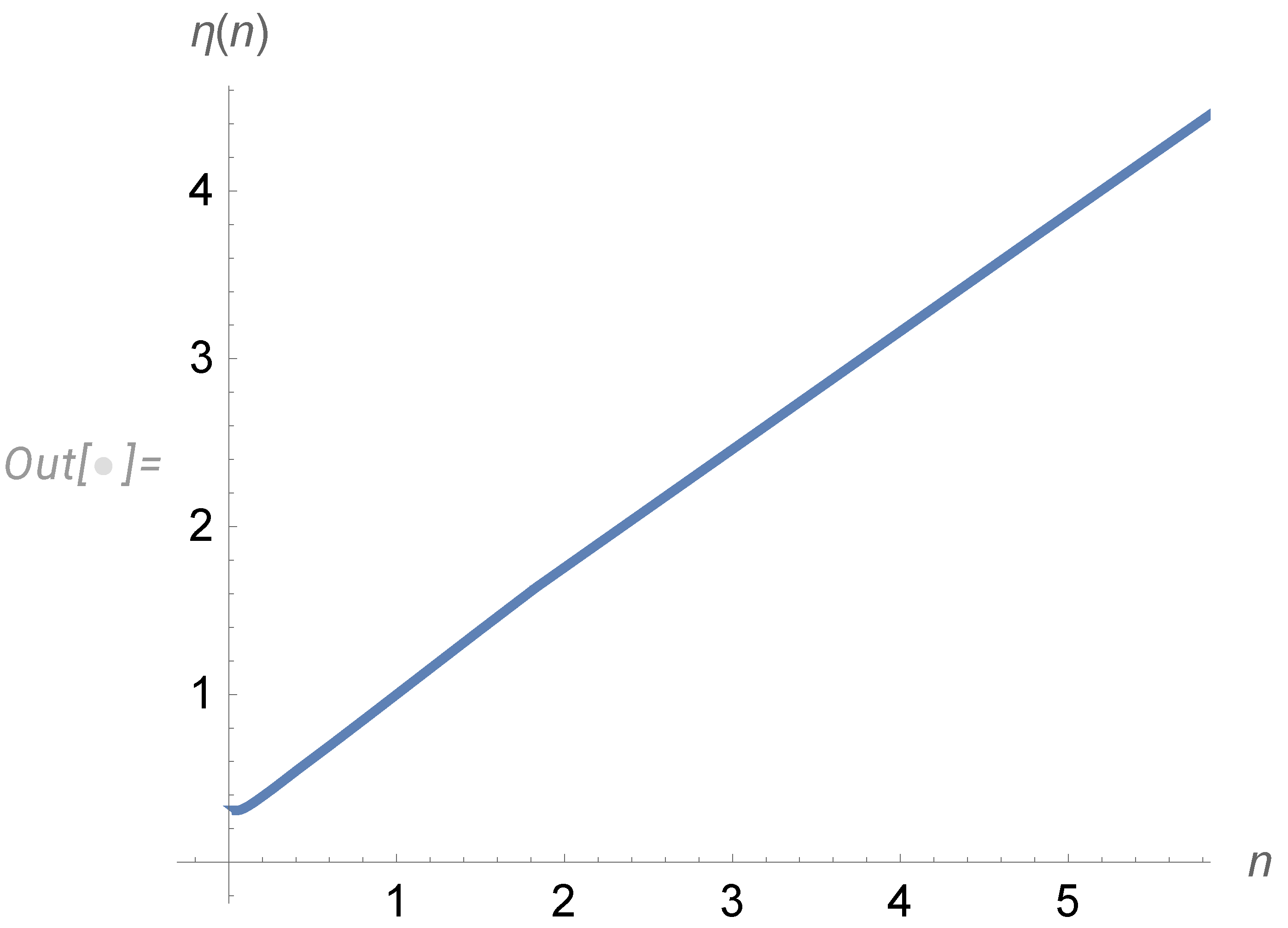
This function was computed in [7], and here is the plot in Figure 6. It is numerically close to a linear function , though it is analytically nonlinear.
We also study some quantum fractal phenomena in the next section. The observable variables are distributed with quantum jumps, not fitting the multifractal framework.
There is another variable that depends on two spins at two different points σ n , σ m , n < m
Y ( p , q , σ ) = σ n σ m X ( p , q )
The even moments Y 2 l of the distribution of Y are the same as those for X, but the odd moments are different:
Y 2 l + 1 = X 2 l + 1 σ n σ m σ E
The analytic computation of the constrained average over sigmas by Mathematica® yields
σ n σ m σ = N q 2 r 2 ( N 1 ) N
We find the following result for the distribution of Y on the whole real axis
f Y ( Y N , q , r ) = 1 2 + sign Y N q 2 r 2 2 ( N 1 ) N f X ( | Y | )
Asymptotically, at s = q r / N 1 we have
f Y ( Y s ) 1 sign ( Y ) s 2 2 ( 1 α ) δ ( | Y | 0 + ) + π Φ 1 π | Y | ;
Due to kinematical restrictions | y | < 1 , our probably stays positive. At r = 0 , we have a special case
f Y ( Y s = 0 ) N + sign ( Y ) 2 N ( 1 α ) δ ( | Y | 0 + ) + π Φ 1 π | Y | ;

4. Vorticity correlation

4.1. Exact relation with conditional probability density

The simplest observable quantities we can extract from the loop functional are the vorticity correlation functions [8], corresponding to the loop C backtracking between two points in space r 1 = 0 , r 2 = r , (see [4] for details and the justification). The vorticity operators are inserted at these two points.
The correlation function reduces to the following average over the big Euler ensemble E of our random curves in complex space [4]
  ω ( 0 ) · ω ( r ) =
1 4 ( t + t 0 ) 2 O ( 3 ) d Ω 0 n < m < N ω m · ω n exp ı ρ · Ω · S n , m S m , n E ;
S n , m = k = n m 1 F k m n ( mod N ) ;
ω k = 0 , 0 , ı σ k 2 cot β 2 ;
ρ = r 2 ν ( t + t 0 ) ;
X [ σ . . . ] p , q , r E X [ σ . . . ] δ [ q r σ ] E δ [ q r σ ] ;
Integrating the global rotation matrix O ( 3 ) is part of the ensemble averaging.
These formulas simplify in the Fourier space, corresponding to the correlation of ω ( k ) · ω ( k ) .
ω ( k ) · ω ( k ) ν 3 2 ( t + t 0 ) 1 2 0 n < m < N ω m · ω n O ( 3 ) d Ω δ 3 Ω · S n , m S m , n k ν ( t + t 0 ) E
This three-dimensional delta function disappears if we introduce the above distribution f Y ( y ) for Y = q 2 ω m · ω n and conditional distribution f Z ( Z y ) for the second variable Z = S n , m S m , n q given the first one y. We rely on r = 0 and even N to dominate the partition function, as it was conjectured in [4] and proven in [6]. We also assume the distribution f Z ( z y ) for the second scaling variable Z, conditional by | Y | = y , to be independent of the sign of Y. The heuristic argument is that the sign of Y depends only on σ n σ m , only two out of N variables σ l , which becomes statistically insignificant at large N.Our large-scale numerical simulation confirms this heuristic argument for N = 2 10 8 .
We also use the conditional probability, which is an integral of the conditional distribution
f Z ( z Y > y ) = y 0 d y f Z ( z y ) ; ;
f Z ( z y ) = y f Z ( z Y > y )
In this case, after switching to f Z ( z Y > y ) and integrating by parts we find
ω ( k ) · ω ( k ) ν 3 2 ( t + t 0 ) 1 2 d W ( q ) q 4 f Y ( y ) y d y d Ω d Z f Z ( Z y ) δ 3 Ω · 0 , 0 , Z q k ν ( t + t 0 ) = ν k 2 ( t + t 0 ) 3 2 d q Φ ( q ) q d y f Y ( y ) y f Z | k | ν ( t + t 0 ) q y = ν k 2 ( t + t 0 ) 3 2 d q Φ ( q ) q d y f Z | k | ν ( t + t 0 ) q Y > y y f Y ( y 0 ) y ;
The distribution f y ( y 0 ) was found above, in (59) by the number theory methods. We are using the derivative
y ( f Y ( y 0 ) y ) = π | y | Φ 1 π | y | y = π Φ 1 π | y | + 2 π 3 n = 1 φ ( n ) n 5 δ y 1 π 2 n 2
The resulting formula for the correlation function
  ω ( k ) · ω ( k ) ν k 2 ( t + t 0 ) 3 2 d q q Φ ( q )
2 π 3 n = 1 φ ( n ) n 5 f Z z Y < 1 π 2 n 2 + π n = 1 Φ ( n + 1 ) 1 π 2 ( n + 1 ) 2 1 π 2 n 2 d y f Z ( z Y < y ) ;
z = | k | ν ( t + t 0 ) q ;

4.2. Extracting conditional distribution from numerical data

We measured conditional probability in our data set of 167 , 772 , 160 samples for N = 200 , 000 , 000 (see Figure 7).
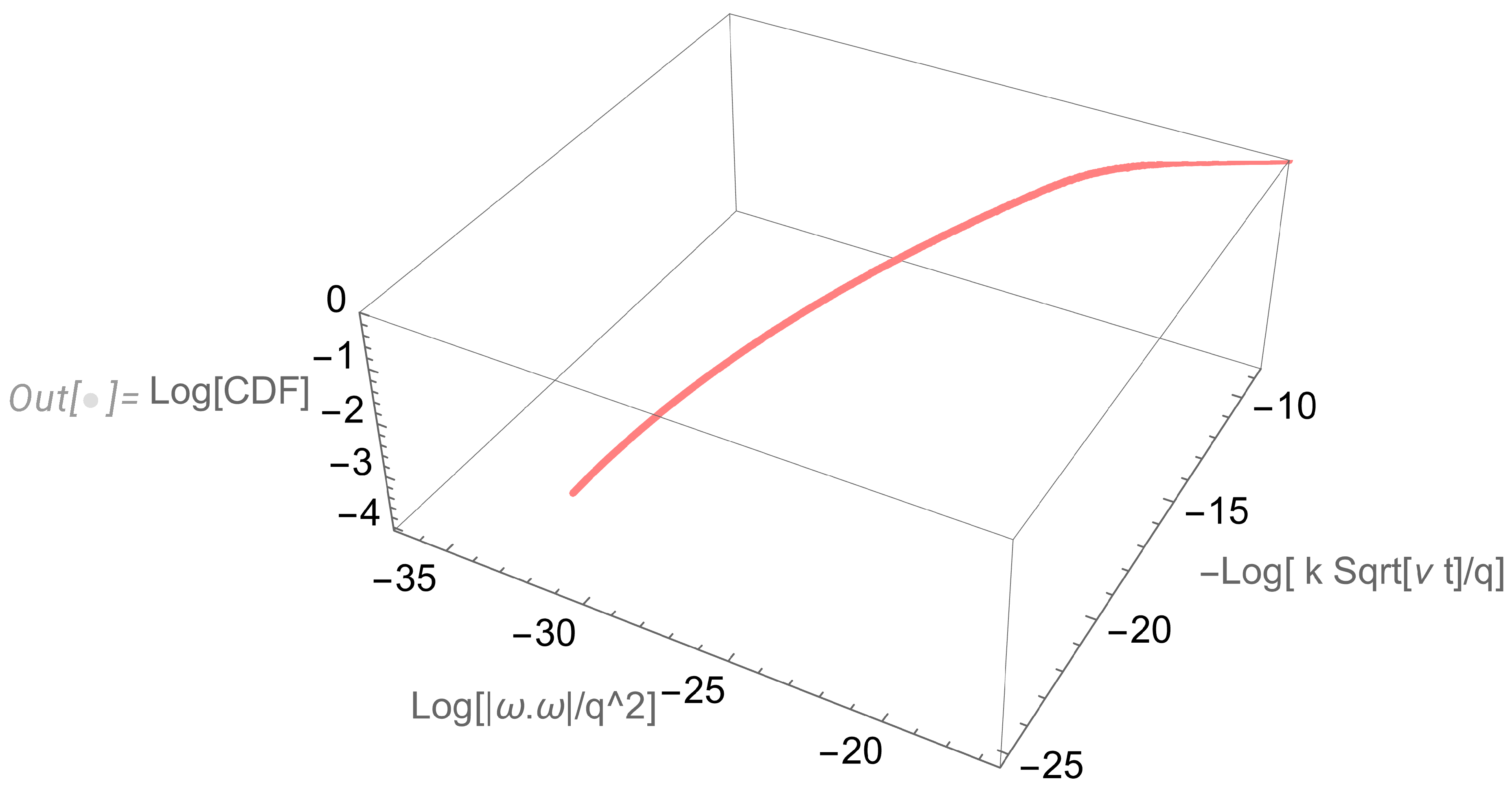
The conditional probability P D S W W < y was defined as a rate of events with given D S and W W < y . It is shown as a 3D plot on the log-log-log scale in Figure 7.
In a classical fractal system, one would expect to observe the two-dimensional surface P log Z log W W < Y in a three-dimensional space Y , Z , P .
Instead, we found a thin, smooth line in three dimensions, which can be fitted as a parametric equation
  log Y = a + b log Z ;
log Z = f ( L ) ;
log P Z W W > Y = L ;
f ( L ) f 0 + f 1 L + f 2 L 2 + f 3 L 3 ;
Projections of this line on three planes reveal its simplicity.
The relation between log Z , log P is shown in Figure 8.
The fit parameter table for f ( x ) is
  Estimate Standard Error t - Statistic P - Value f 0 10.6123 0.0030473 3482.54 0 . f 1 5.43603 0.00542859 1001.37 0 . f 2 0.849258 0.00224021 379.097 0 . f 3 0.0500626 0.000234038 213.908 0 .
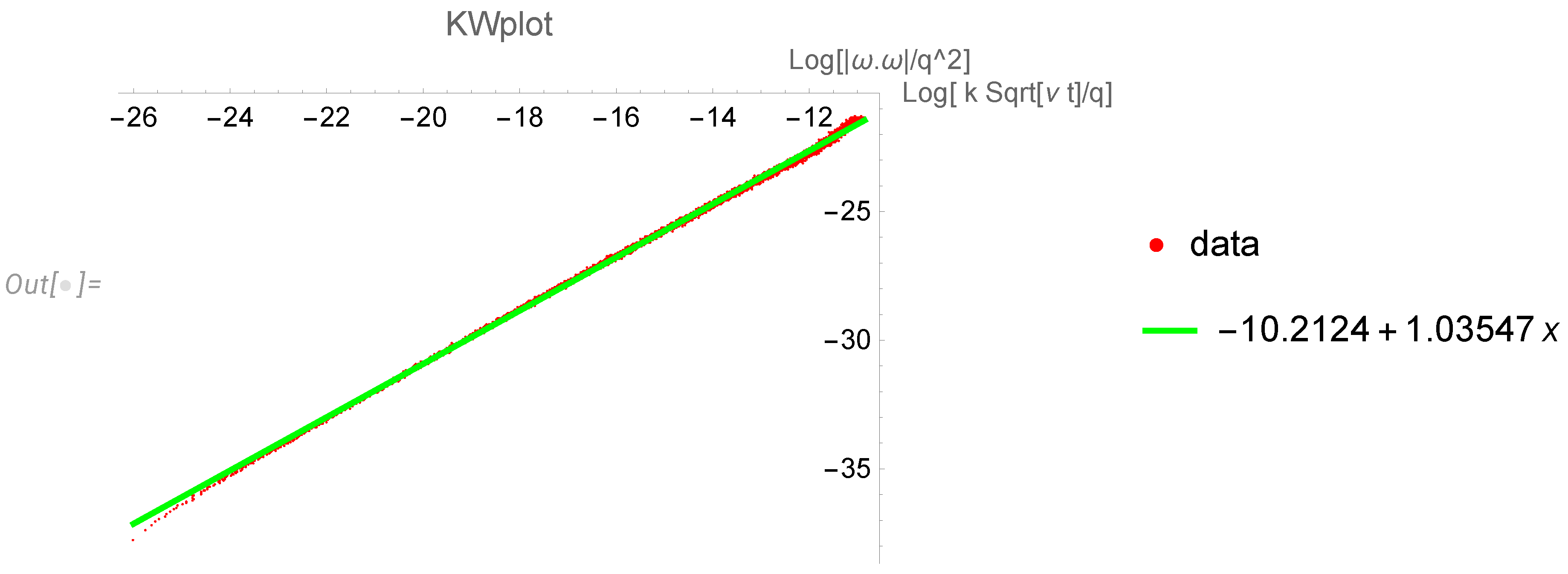
If we directly plot Y ( Z ) , we get a straight line corresponding to a scaling law (see Figure 9). The fitting table for this linear relation log Y = a + b log Z in the log-log scale is
  Estimate Standard Error t - Statistic P - Value a 10.2124 0.0039544 2582.54 0 . b 1.03547 0.00025789 4015.16 0 .
So, a scaling law is hidden inside the discontinuous distributions induced by Euler totients.
  Y = A Z b ;
A = exp a = 0.0000367128 ;
The probability density f Z ( z Y > y ) , which we need in correlation function, is related to this number of events P Z W W > y as follows
f Z ( z Y > y ) = d P Z W W > y d Z = L P Z W W > y L Z = exp L f ( L ) | f ( L ) |

4.3. Final results for the energy spectrum

We use parametric representation (72) and transform the integral, inverting relation between L and log K / q (see details in [7]).
We arrive at the following correlation
  ω · ω ( k ) = ν 2 ν ( t + t 0 ) G N ( K ) H ( K ) / K ;
K = | k | ν ( t + t 0 ) ;
G N ( K ) = K N q 2 Φ q exp L ( q / K ) | f ( L ( q / K ) ) | d q ;
L ( q / k ) = f 1 ( log K / q ) ;
H ( K ) = 2 π 3 n = 1 ϕ ( n ) n 5 δ A K b 1 n 2 π 2 + π Φ 1 A K b π ;
Here w = f 1 ( ξ ) is the real root of equation f ( w ) = ξ . In our case ξ = log ( K / q ) , and f 1 ( ξ ) ξ 1 3 ( log q ) 1 3 These estimates show that function G N ( K ) in continuum limit N tends to a constant, independent of K, but growing with N
G N ( K ) F ( N )
This work neglects such normalization factors, not affecting the energy spectrum. We restore normalization, comparing our dissipation with the exact result from [4].
The summation n in H(K) at any given K selects only one term with a quantized spectrum in the energy
E ( k , t ) k 2 v · v ( k ) ω · ω ( k ) ν 2 ν ( t + t 0 ) H ( K ) / K ;
The spectrum has delta function peaks at
  K n = 1 ( A n 2 π 2 ) 1 b , n = 1 , 2 , ;
| k | n = K n ν ( t + t 0 ) ;
The whole spectrum support lies at K < K 1 ; otherwise, both terms in H ( K ) vanish. The critical region is K 0 , which means the smaller and smaller wavevectors at larger and larger times. In the limit K 0
H ( K ) / K 1 K b + 1 ;
E ( k , t ) F ( N ) ν 2 | k | b + 1 ( ν ( t + t 0 ) ) 1 + b / 2 ;
This asymptotic power spectrum is only part of the story. There is a maximal time for any wavevector
t m a x ( k ) = t 0 + K 1 2 ν k 2
The decay stops at this wavelength after this moment, as H ( K > K 1 ) = 0 .
The quantum effects lead to peaks and jumps at finite K = k ν ( t + t 0 ) . Only the average over a large range of the spectrum approaches the scaling law.
The integral over k leads to a simple power law for the energy dissipation rate
E 4 π ( 2 π ) 3 0 d k k 2 ω · ω ( k ) ν 2 2 π 2 ν ( t + t 0 ) 0 d k k H k ν ( t + t 0 ) = 0 K 1 K d K H ( K ) 2 π 2 ( t + t 0 ) 2
This law agrees with the exact computation of the same quantity made in [4]. Comparing coefficients in front of ( t + t 0 ) 2 , one can restore the missing normalization factor in our energy spectrum.
E ( k , t ) = ω · ω ( k ) = 35 π 4 1728 ζ ( 3 ) μ 2 ν | k | ( t + t 0 ) H | k | ν ( t + t 0 ) 0 K 1 x d x H ( x )
where μ ν 0 is the chemical potential introduced in [4].
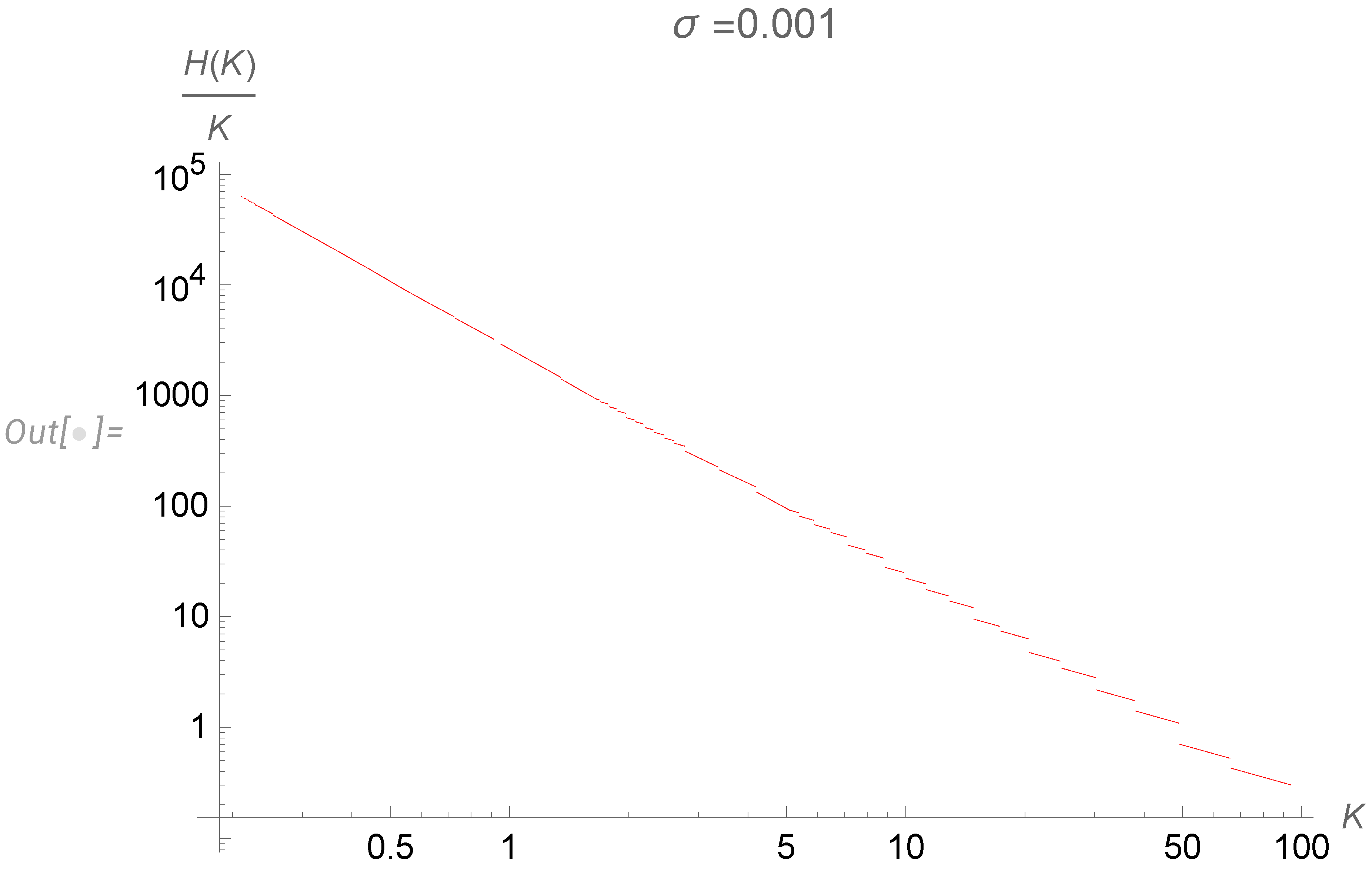
Finally, let us plot the universal function H ( K ) / K , using a width σ = 10 3 for normal distribution instead of a pure delta function with σ = 0 (see Figure 10). The narrow peaks at the K = K n are not visible because of the very small heights of these peaks. The curve has tilted steps with diminishing width as K 0 . The local slope is K 1 , but the average slope over wide range is K 1 b K 2.03 .

5. Conclusions

There are several new results reported in this paper.
  • Continuum limit of distribution of scaling variables (34),(39) in the small Euler ensemble.
  • Relation between the vorticity correlation and conditional probability distribution f Z ( z Y ) .
  • Fast algorithm with O ( 1 ) memory to simulate the big Euler ensemble as a Markov chain.
  • The scaling law (78) for the conditional probability leads to the discrete energy spectrum (88) on top of a continuous background in (81).
  • The decay at a given time goes only at small enough wavelengths. At a fixed wavelength, the decay stops after some critical time, inversely proportional to the wavelength.
Nothing like these quantum effects was observed in numerical simulations [9]. There could be several explanations (see discussion in the paper [10]). It is very difficult to numerically distinguish the devil’s staircase like that in Figure 10 from the good old power law.
Discrete energy spectrum in classical turbulence sounds like heresy, though it does not contradict any known fluid dynamics principles. Let us stress that we did not assume a discrete spectrum: it came from large-scale simulations on a supercomputer with very small statistical errors and some exact distributions derived from the number theory.
This discrete spectrum stems from the exact analogy between decaying turbulence and the quantum mechanics in loop space [1,4,8].
We would like to hear the response from leading experts in fluid dynamics before finally publishing this paper in a journal.

Data Availability Statement

We generated new data for the vorticity distribution using the Mathematica® code [7] and Python/CPP code [11]. All this code is available for download.

Acknowledgments

Maxim Bulatov helped me with the derivation of the Cotangent sums, and also with the fast code for the GPU cluster. I am grateful to Maxim for that. This research was supported by a Simons Foundation award ID 686282 at NYU Abu Dhabi. The computations were done on the High-Performance Computing resources at New York University Abu Dhabi.

Appendix A. The cotangent sum and Jordan totients.

The Euler ensemble expectation value of cot 2 π p q can be reduced to the prime numbers as follows. We start with an unconstrained sum, which is elementary [12].
n = 1 m 1 cot 2 π n m = 1 3 m 2 m + 2 3
Let us consider a sum G [ F , m ] of arbitrary function F ( n / m ) constrained to the coprime n , m . In our case
F ( x ) = 0 if x = 1 cot 2 π x otherwise
Such sum satisfies the following equation (with p 1 < p 2 < p S denoting S ordered prime factors of m and ( n , m ) denoting coprime n , m ).
m = s = 1 S p s α s ;
G [ F , m ] = n = 1 ( n , m ) = 1 m F ( n / m ) ;
H ( m ) = n = 1 m F ( n / m ) ;
  G [ F , m ] = H ( m ) + s = 1 S ( 1 ) s 0 < l 1 < l 2 < l s S H m p l 1 p l 2 p l s ;
Let us go into detail. Consider the first term for particular l 1 = l , p ( l 1 ) = p
H ( m ) H m p = n = 1 m F ( n / m ) n = 1 m F ( n / m ) m = m / p = n = 1 m F ( n / m ) n = 1 n ( mod p ) = 0 m F ( n / m )
We observe that the second term removes from the total sum n = 1 m in the first term all the terms with n ( mod p ) = 0 . In the same way, the other terms in the sum l H m p l remove all the terms in the first sum with ( n , m ) = p l . However, there are terms in n = 1 m F ( n / m ) like n = p 1 p 2 , which are proportional to two prime factors p 1 , p 2 , and we removed these terms twice, once in the term H m p 1 and the second time in H m p 2 . So, we have to add them back, with + 1 sign for each pair p i , p j . This addition provides the next term with double sum 0 < l 1 < l 2 S .
In general, this formula is a particular case of the inclusion-exclusion principle [13]. As the basic equation (A6) is a linear functional of H, we can solve this equation separately for H l ( m ) = m l , and then by adding these solutions with proper coefficients, we get the solution for our particular H ( m ) = 2 3 m + 1 3 m 2 . Let us start with the simplest case, H 1 ( m ) = m . The solution is the Euler φ ( m ) . Here is how the equation is satisfied:
G 1 ( m ) = m + m s = 1 S ( 1 ) s 0 < l 1 < l 2 < l s S 1 p l 1 p l 2 p l s = m l = 1 S 1 1 p l
The next case, G 2 ( m ) is processed the same way, with the result
G 2 ( m ) = m 2 s = 0 L ( 1 ) s l 1 < l 2 < l s 1 p 2 ( l 1 ) p 2 ( l 2 ) p 2 ( l s ) = m 2 l = 1 L 1 1 p l 2
Finally, the function G 0 ( m )
G 0 ( m ) = s = 0 S ( 1 ) s l 1 < l 2 < l s 1 = s = 0 S ( 1 ) s S s = ( 1 1 ) S = 0
Putting all together
S ( m ) = n = 1 ( n , m ) m 1 cot 2 π n m = 1 3 J 2 ( m ) J 1 ( m ) ;
J l ( m ) = m l p | m 1 1 p l ;
Jordan introduced these generalized totients [14] J l ( m ) in 1870. The asymptotic behavior of the Jordan totient summatory functions is known:
m = 2 N J l ( m ) N l + 1 ( l + 1 ) ζ ( l + 1 )

Appendix B. Algorithms.

The numerical simulation of the correlation function does not require significant computer resources. It is like a simulation of a one-dimensional Ising model with long-range forces. However, a much more efficient method is to simulate the Markov process, equivalent to the Fermionic trace of the [10].
Regarding that quantum trace, we are simulating the random histories of the changes of the Fermionic occupation numbers, taking each step off history with Markov matrix probabilities.
We devised an algorithm that does not take computer memory growing with the number N of points at the fractal curve. This algorithm works for very large N 10 9 , and it can be executed on the GPU in the supercomputer cluster, expanding the statistics of the simulation by massive parallelization.
We use large values of N = 2 10 8 . As for the random values of fractions p q with 0 < p < q < N , we used the following Python algorithm.
We used even N , q and N ± = N / 2 , as it was shown in [4] that these are the dominant values in the local limit μ 0 .
Preprints 93832 i001
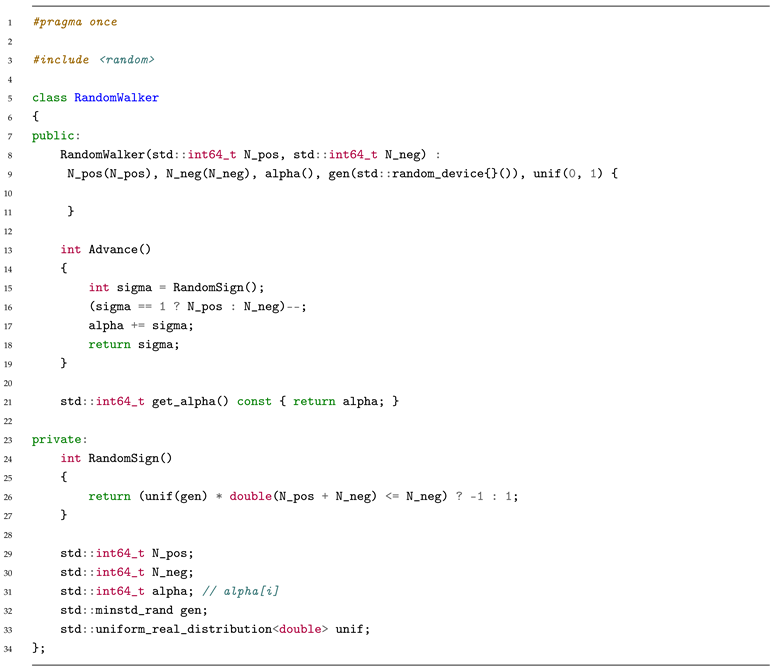
In other words, we generated random even q ( 2 , N ) , after which we tried random 0 < p < q until we got a coprime pair ( p , q ) . Statistically, at large N, this happens with probability 6 / π 2 0.61 (see [15]). On average, it takes π 2 / 6 1.64493 attempts to get a coprime pair.
Once we have a p candidate, we accept it with the chance w = q N , which, again, for large q N has a finite acceptance rate. The probabilities multiply to the desired factor, which is proportional to Euler totient
P ( ( p , q ) = 1 ; p < q ) = φ ( q ) q ;
φ ( q ) q P ( random ( 1 , N ) < q ) = φ ( q ) N ;
The main task is to generate a sequence of random spins σ 1 = ± 1 , σ N = ± 1 with prescribed numbers N + , N of + 1 and 1 values. The statistical observables are additive and depend upon the partial sums α n = k < n σ k .
We avoid storing arrays of σ k , α k , using iterative methods to compute these observables. Our RAM will not grow with N, with CPU time growing only linearly.
The C++ class RandomWalker generates this stream of σ k , α k .
Preprints 93832 i002
At each consecutive step, the random sign σ = ± 1 is generated with probabilities n + n + + n , n n + + n after which the corresponding number n + or n is decremented, starting with n ± = N ± at step zero. By construction, in the end, there will be precisely N + positive and N negative random values σ k .
This algorithm describes a Markov chain corresponding to sequential drawing random σ from the set with initial N ± positive and negative spins, and equivalent to one-dimensional random walk on a number line. These conditional probabilities
P σ k = 1 | σ 1 σ k 1 = n + n + + n ;
n ± = l < k 1 ± σ l 2
are such that unconditional probability equals to the correct value:
P σ k = 1 | σ 1 σ k 1 σ 1 σ k 1 = P σ k = 1 = N + N + + N ;
regardless of the position k of the variable σ k at the chain.
The formal proof goes as follows.
Proof. 
At k = 1 , without spins to the left on the chain, the conditional probability equals the total probability, and the statement holds. With some number of spins on the left, averaging over all these spins at a fixed value of σ k is equivalent to averaging over all values except σ k because the only condition on random spins is their net sum, which is a symmetric function of their values. Thus, the average of conditional probabilities equals the total probability (A18) for any spin on the chain, not just the first one. □
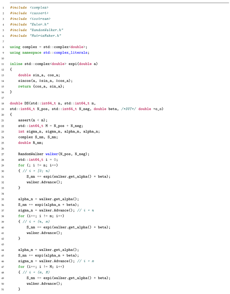
Here is the code, which computes the sample of | d S n m | , ω · ω given n , m , N + , N , β . The 2D vectors S are treated as complex numbers, using 128 bit complex arithmetic.
Preprints 93832 i003a
Preprints 93832 i003b
This code fits the architecture of the supercomputer cluster with many GPU units at each node. These GPU units are aggregated in blocks by 32, with every init inside the block working in sync. We use this synchronization to collect statistics: every block is assigned with different random values of n , m , N + , N , β , and every unit inside the block performs the same computation of DS function with different values of the integer seed for the random number generator, automatically provided by the system.
When quantum computers become a reality, our sum over the sum of the Markov history of discrete spin (or Fermion) variables will run massively parallel on the qubits. Our Euler/Markov ensemble is ideally suited for quantum computers.

Appendix C. The O(3) group average
The correlation function (60) involves an integral over the O ( 3 ) group
Q ( r , s ) = O ( 3 ) d Ω | O ( 3 ) | exp ı r · O ^ · s ;
with the vector s related to our fractal curve F ( θ ) in a particular sample in our ensemble.
Both vectors r , s are real.
This integral is a particular case of a Harish-Chandra-Itzykson-Zuber integral formula [16],
U ( n ) e tr ( A U B U ) d U = p = 1 n 1 p ! det e a i b j Δ ( A ) Δ ( B )
where
Δ ( A ) = i < j ( a j a i )
is the Vandermonde determinant.
In our case, O ( 3 ) =   S U ( 2 ) / Z 2 , so we use n = 2 formula with
A = ı σ i r i , Δ ( A ) = 2 ı | r |
B = σ j s j , Δ ( B ) = 2 | s |
det e a i b j = 2 ı sin | r | | s |
where σ are Pauli matrices. With proper normalization to 1 at r = 0 , the HCIZ integral reads
O ( 3 ) d Ω | O ( 3 ) | exp ı r · O ^ · s = sin | r | | s | | r | | s |
Next, let us consider the case of the Fourier integral needed for the Wilson loop.
The group integration is now involved in the averaging of the ensemble of our random loops F k with vector steps q k = F k + 1 F k :
  O ( 3 ) d Ω | O ( 3 ) | exp ı k = 1 N C ( 2 π k / N ) · Ω ^ · q k 2 ν ( t + t 0 ) =
O ( 3 ) d Ω | O ( 3 ) | exp ı tr Ω ^ · X ^ ;
X ^ = k = 1 N q k C ( 2 π k / N ) 2 ν ( t + t 0 )
The matrix X ^ is not symmetric but real, as the vectors q k are real. These are unit vectors on a plane, equivalent to complex numbers
  q ^ k = q k , x + ı q k , y = ı σ k exp ı β σ k 2 l = 0 k 1 exp ı β σ l ;
This integral does not reduce to the HCIZ integral and needs special treatment.
We use a quaternionic representation of O ( 3 ) and write this integral:
Q ( X ^ ) = S 3 ( d x ) | S 3 | exp ı x λ x ρ R λ ρ ;
  R λ ρ = 1 2 T i j λ ρ + T i j ρ λ X i j ;
T i j α β = 1 2 tr σ i τ α σ j τ β ;
τ α = { 1 , ı σ } ; α = ( 0 , 1 , 2 , 3 ) ;
x α 2 = 1
In this representation, we have full O ( 4 ) symmetry of this integral over unit sphere S 3 in four dimensions, plus there is a symmetry of the tensor R α β = R β α .
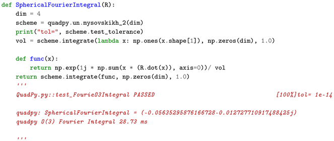
This Fourier integral can be computed in tens of milliseconds using a fast Python library quadpy[17]. It is optimized for integration over geometric shapes, including spheres in arbitrary dimensions. We licensed this library from the author and used it for our computations. Here is the code with its output for a random real symmetric tensor R
Preprints 93832 i004

References

  1. Migdal, A. Loop Equation and Area Law in Turbulence. In Quantum Field Theory and String Theory; Baulieu, L.; Dotsenko, V.; Kazakov, V.; Windey, P., Eds.; Springer US, 1995; pp. 193–231. [CrossRef]
  2. Makeenko, Y.; Migdal, A. Exact equation for the loop average in multicolor QCD. Physics Letters B 1979, 88, 135–137. [Google Scholar] [CrossRef]
  3. Migdal, A. Loop equations and 1N expansion. Physics Reports 1983, 201. [Google Scholar] [CrossRef]
  4. Migdal, A. To the Theory of Decaying Turbulence. Fractal and Fractional 2023, arXiv:physics.flu-dyn/2304.13719]7, 754. [Google Scholar] [CrossRef]
  5. Hardy, G.H.; Wright, E.M. An introduction to the theory of numbers, sixth ed.; Oxford University Press, Oxford, 2008; pp. xxii+621. Revised by D. R. Heath-Brown and J. H. Silverman, With a foreword by Andrew Wiles.
  6. Basak, D.; Zaharescu, A. Connections between Number Theory and the theory of Turbulence, 2024. To be published.
  7. Migdal, A. "NumericalAnalysisOfEulerEnsembleInDecayingTurbulence". "https://www.wolframcloud.com/obj/sasha.migdal/Published/NumericalAnalysisOfEulerEnsembleInDecayingTurbulence.nb", 2023.
  8. Migdal, A. Statistical Equilibrium of Circulating Fluids. Physics Reports 2023, arXiv:physics.flu-dyn/2209.12312]1011C, 1–117. [Google Scholar] [CrossRef]
  9. Sreenivasan, K.R. On the scaling of the turbulence energy dissipation rate. The Physics of Fluids 1984, 27, 1048–1051. [Google Scholar] [CrossRef]
  10. Migdal, A. Dual Theory of Decaying Turbulence: 1: Fermionic Representation., 2023.
  11. Migdal, A. LoopEquations. https://github.com/sashamigdal/LoopEquations.git, 2023.
  12. Migdal, A. Decaying Turbulence Computations. https://www.wolframcloud.com/obj/sasha.migdal/Published/DecayingTurbulenceComputations.nb, 2023.
  13. Cioabă, S.M.; Murty, M.R. The Principle of Inclusion and Exclusion. In A First Course in Graph Theory and Combinatorics: Second Edition; Springer Nature Singapore: Singapore, 2022; pp. 33–42. [Google Scholar] [CrossRef]
  14. Moree, P.; Saad Eddin, S.; Sedunova, A.; Suzuki, Y. Jordan totient quotients. Journal of Number Theory 2020, 209, 147–166. [Google Scholar] [CrossRef]
  15. Lei, J.; Kadane, J.B. On the probability that two random integers are coprime, 2019. arXiv:math.PR/1806.00053.
  16. McSwiggen, C. The Harish-Chandra integral: An introduction with examples, 2021. arXiv:math-ph/1806.11155.
  17. Schlömer, N. QuadPy. https://github.com/sigma-py/quadpy.git, 2023.
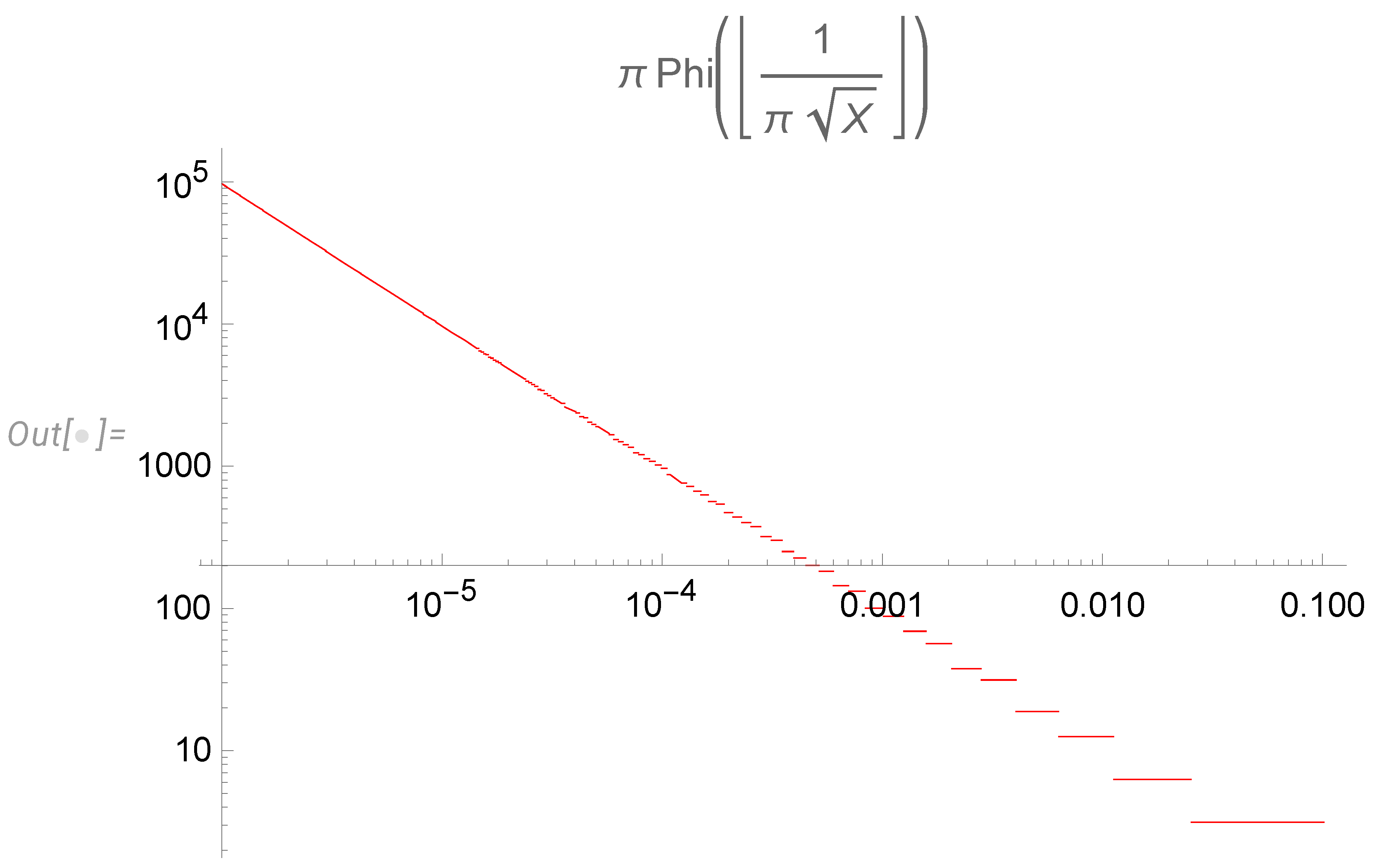
Figure 1. The log-log-plot of the totient summatory function. It is takes a constant value φ ( k ) π at each internal 1 π 2 ( k + 1 ) 2 < X < 1 π 2 k 2 with positive integer k. The convergent integral α = 0.387153 of this piecewise constant function reduces to the sum of these constant values times the widths of the intervals.
Preprints 93832 g001
Figure 2. The CDF for p q for positive and negative ω m · ω n
Preprints 93832 g002
Figure 3. Log-log plot of CDF tail for S n , m S m , n / q . The curve is nonlinear in log scale, contradicting the simple fractal scaling laws.
Preprints 93832 g003
Figure 4. Log-log plot of CDF tail for ω m · ω n / q 2 . The curve is nonlinear in log scale, contradicting the simple fractal scaling laws.
Preprints 93832 g004
Figure 5. Fit of log ( 1 C D F ( D S ) ) with 20 Chebyshev polynomials of log D S rescaled to 1 , 1 interval. The small statistics data at large negative log D S was discarded
Preprints 93832 g005
Figure 6. The multifractal dimension η ( n ) of moments D S n . The curve is numerically close to a linear function.
Preprints 93832 g006
Figure 7. 3D Plot of the conditional probability P log D S log W W < y in a triple log scale. The data (red dots) was averaged over 1000 samples sorted by log W W .
Preprints 93832 g007
Figure 8. The relation of log Z , log P (red dots) is fitted by a third-degree polynomial (blue)
Preprints 93832 g008
Figure 9. Direct scaling relation between W W and D S , ads fit to the log-log of joint distribution
Preprints 93832 g009
Figure 10. The log-log plot of H ( K ) / K as a function of K = | k | ν ( t + t 0 ) . For display purposes, the delta function was replaced by the normal distribution PDF with σ = 10 3 . This change did not affect the curve, as these discrete spectrum peaks are numerically very small.
Preprints 93832 g010
Disclaimer/Publisher’s Note: The statements, opinions and data contained in all publications are solely those of the individual author(s) and contributor(s) and not of MDPI and/or the editor(s). MDPI and/or the editor(s) disclaim responsibility for any injury to people or property resulting from any ideas, methods, instructions or products referred to in the content.
Copyright: This open access article is published under a Creative Commons CC BY 4.0 license, which permit the free download, distribution, and reuse, provided that the author and preprint are cited in any reuse.
Alerts
Prerpints.org logo

Preprints.org is a free preprint server supported by MDPI in Basel, Switzerland.

Subscribe

© 2025 MDPI (Basel, Switzerland) unless otherwise stated