
Submitted:
13 September 2024
Posted:
16 September 2024
You are already at the latest version
Abstract
Several stochastic H∞ filters for estimating the attitude of a rigid body from line-of-sight measurements and rate gyro readings are developed. The measurements are corrupted by white noise with unknown variances. Our approach consists of estimating the quaternion while attenuating the transmission gain from the unknown variances and initial errors to the current estimation error. The time-varying H∞ gains are computed through differential and algebraic linear matrix inequalities whose parameters are independent of the state. The case of a gyro drift is addressed, too. Extensive Monte Carlo simulations show that the proposed stochastic H∞ quaternion filters perform well for a wide range of noise variances. The actual attenuation, which improves with the noise level and is worst in the noise-free case, is better than the guaranteed attenuation by one order of magnitude. The proposed stochastic H∞ filter produces smaller biases than a standard quaternion Kalman filter and similar standard deviations at large noise levels. An essential advantage of this H∞ filter is that the gains are independent of the quaternion, which makes it insensitive to modeling errors. This desired feature is illustrated by comparing its performances against those of unmatched Kalman filters. When provided with too high or too low noise variances the Kalman filter is outperformed by the $H_\infty$ filter, which essentially delivers identical error magnitudes.
Keywords:
Stochastic H∞ filtering
; Attitude determination
; Quaternion
; Uncertain sensor variance
1. Introduction
The attitude quaternion [1][p. 758] is a very popular spacecraft attitude parametrization, whose mathematical modeling and filtering have been ongoing topics of research for more than four decades [2]. Numerous successful quaternion stochastic estimators have been developed in the realm of optimal filtering, e.g. [3,4] and [5, Ch. 6] for an in-depth survey. An inherent drawback of the optimal filtering approach consists in its sensitivity to the model noise variance. Although adapting the filter gain computations might provide satisfactory performances in some cases, like adaptive process noise estimation in [6] and uncompensated random biases in [7,8], the designer might prefer a less sensitive approach: rather than trying to estimate the unknown parameters, the filter shall attenuate their impact on the estimation error for a transmission level that should be as small as possible. This general approach was followed in [9,10,11] for spacecraft attitude determination. In [9] an estimator of the spacecraft quaternion and gyro biases was developed. In [10,11] extended filters were applied to spacecraft attitude determination and gyro calibration by processing space-borne telemetry of the CBERS-2 satellite, including outputs from rate gyros, two sun sensors, and an earth’s sensor. The filters produced estimates of Euler angles and the quaternion, respectively, along with estimates of the gyro biases. Their performance compared favorably with those of standard extended Kalman filters. Reference [12] presented an invariant extended filter for attitude and position estimation using Lie groups algebra, which conveniently produces state-independent Jacobians at any linearization point. All the above works are rooted in the deterministic estimation theory. In that realm, the measurement and process noises, and the initial errors, are modeled as energy-finite disturbances, a.k.a. or signals.
In this work, stochastic quaternion filters are developed for models with process and measurement white noise rather than finite-energy disturbances. We assume that a time-varying line-of-sight (LOS) signal is continuously acquired, that a triad of body-mounted gyros provides a measurement of the spacecraft’s angular velocity, and that both measurement processes are corrupted by additive white noise. The case of a gyro bias is addressed through Brownian motion modeling. All white noise variances are assumed to be unknown. A distinctive feature of our modeling and filtering approach is that the plant equations admit white noise as inputs and that their variances are assumed to be finite-energy perturbations. The stochastic filter aims at estimating the quaternion while attenuating these perturbations. This article is a revised and expanded version of a paper [16] which was presented at the AIAA Guidance Navigation and Control Conference, Toronto, Ontario, Canada, 2010. It is here extended to include the development of an filter for quaternion and gyro bias estimation, along with extensive Monte-Carlo simulations for validation. The proposed approach is inspired by works on stochastic filtering and control for nonlinear systems, which are grounded in dissipativity theory [13,14].
Several filters are developed: first, the gyro noise variance is the sole unknown, then both the gyro and the LOS noise variances are unknown, and finally the case of biased gyro measurements is considered. The state multiplicative nature of the errors in both the process and measurement provides a useful structure to the model. The proposed approach avoids linearization by exploiting a pseudo-linear quaternion plant model, which was introduced in [6] and extended to continuous-time stochastic settings in [15]. The filter implementation requires solving differential linear matrix inequalities that do not depend on the state estimate. Extensive Monte-Carlo simulations were run in order to evaluate the novel filter’s performances as an attitude estimator, and to compare them with those of a quaternion multiplicative extended Kalman filter.
2. Quaternion Stochastic Filtering
2.1. Problem statement
For the sake of simplicity and clarity, the case of drift-free gyroscopes is treated first. Consider the following Itô stochastic differential equation (SDE) for the attitude quaternion, and the associated measurement equation [15]:
where denotes the attitude quaternion, is the following matrix function of the measured angular velocity ,
where , which is acquired by a triad of body-mounted gyroscopes, is corrupted by an additive standard Brownian motion, , with infinitesimal independent increments such that . The parameter denotes the standard deviation of the gyro noise . The drift term in Eq. (1) features a damping term in that ensures mean-square stability of the process . Equation (2) is a continuous-time quaternion measurement equation where the measurement value is identically zero [6]. Hence,
and the measurement matrix is constructed from LOS measurements. Let and denote the projections of a measured LOS in the spacecraft body frame axes and a reference inertial frame, respectively, then is computed as follows
The matrix, , which appears both in the process and measurement multiplicative noises, is the following linear matrix function of the quaternion :
The measurement noise is modeled as a standard Brownian motion, , multiplied by the parameter . Assume that and are unknown, possibly time-varying random parameters, and that there is no prior knowledge of their possible values or bounds. The filtering problem consists of estimating the quaternion in the presence of unknown and random and and is formulated as a disturbance attenuation problem. The following estimator is considered:
The Itô correction term, , is dropped for simplicity. It is not required for the filter development since the dynamics of the filter estimate and estimation error, , are designed to be stable in the mean-square sense independently from that correction [13]. Let denote the additive quaternion estimation error, i.e.,
Given a scalar , a gain process is sought such that the following criterion is satisfied:
under the constraints (1)(2), and where denotes the augmented process of admissible disturbance functions. Whenever Eq. (12) is true, the so-called -gain property from to , is satisfied for . Two cases for will be considered in the following: and and significant differences will be highlighted.
2.2. Augmented stochastic process
Following standard techniques, the following augmented process is defined:
The design model for the process obeys the following equation
The estimator’s equation is given by Eq. (9), i.e.
where denotes . Using Eqs. (14), (15), and (2) yields the SDE for the estimation error:
where denotes the matrix , , , denote the columns of the matrix , and the scalar processes , , are the components of the vector Brownian motion . Notice that is a function of the augmented process since it is a function of the quaternion . and denote the matrices and , respectively, while and , , denote their columns. Appending Eqs. (15) and (16) yields the following augmented SDE:
where denotes an matrix of zeros. Equation (17) can be re-written in the following compact form:
where , and are effectively defined from Eq. (17).
2.3. Hamilton-Jacobi-Bellman inequality
The desired -gain property will be satisfied if and only if the augmented system (18) is dissipative with respect to the supply rate , for a given positive scalar [13]. Thus a non-negative scalar-valued function, , is sought that satisfies the fundamental property [14]:
for all and for all admissible . When Eq. (19) is satisfied, the function V is called a storage function for the supply rate S. A sufficient condition for Eq. (19) is:
for all and for all admissible , where is the Itô differential of the function V. Notice that the processes and are observed and thus belong to the information pattern. Let denote the information pattern at time t, which includes the observations of the angular velocity and of the LOS until t, i.e. . In the development of the sufficiency conditions, one can use the following property of the expectation operator to write (21) as follows:
for all and t. Then a sufficient condition for (22) is
for all and t. Given the conditioning on in (23), the functions and can be considered deterministic functions. Using the Itô differentiation rule [17, p. 112] and dropping the expectation operator on both sides of Eq. (21) yields the following sufficient condition, i.e. the Hamilton-Jacobi-Bellman (HJB) inequality for :
for all , , and for all admissible , where G and are functions of . Dropping the integral and the expectation operators is a standard procedure in stochastic estimation and control [13] or in stochastic optimal control [18, p. 321].
2.3.1. Case where
Assume both and are perturbations. Bringing all terms to the left-hand-side (LHS) of Eq. (24) yields
where L denotes the following matrix
and denotes the four-dimensional identity matrix. For a solution to exist for all and for all admissible the coefficients multiplying the arbitrary disturbance functions, and , in Eq. (25) must be negative, which yields the following conditions:
for all , . Thus, according to Eq. (25), any non-zero disturbance will only add a negative term to the LHS, increasing the system’s dissipativity for the chosen supply rate. Henceforth, the worst-case scenario consists in vanishing disturbances e.g.,
Some interpretation of Eqs. (29),(30) is required. It might appear at first sight counter-intuitive that the worst-case scenario for an estimator consists of vanishing noise variances. However, the proposed solution follows the attenuation criterion (12), not a minimum error condition. Henceforth performance is measured via the ratio between the ( norms of the) estimation error and the noise variance, not via the estimation error itself. It is thus not surprising that the proposed estimator will perform better, i.e. attenuate better in the presence of high variances than in the presence of low variances.
Summary:
2.3.2. Case where
Consider the case where is the sole perturbation. In this case, the HJB inequality evaluated at the worst-case yields the following sufficient conditions: for all and ,
In Eq. (34), the parameter is a known deterministic parameter.
2.4. Storage function V
A standard approach to circumvent the formidable task of solving the partial differential inequality for V [Eq. (24)] consists of guessing the solution in a parameterized form and developing sufficient conditions for its parameters. The classical quadratic form for V will be used here:
where is assumed to be symmetric, positive, and block diagonal, i.e.,
2.5. Sufficient conditions on the matrices , ,
Using Eqs. (36),(37) in Eq. (31), straightforward computations yield the following identity:
where is defined as follows:
Exploiting the following property of the matrix [5, Eq. (8.20b)],
yields the following identities
2.5.1. Convexity condition with respect to
Using Eq. (41) in Eq. (33) [Eq. (35)], and noting that the inequality must be verified for all yields the following condition on :
This condition must be satisfied in both cases, whether is known or is an unknown perturbation. The latter condition can be easily reformulated in terms of the characteristic values of the symmetric positive matrix . Let , , denote the four positive eigenvalues of , then Eq. (43) is equivalent to the following condition:
2.5.2. Case where
Using Eq. (42) in Eq. (32), and noting that the inequality must be verified for all , yields the following condition on and :
Using Eq. (38) in Eq. (31) yields two uncoupled differential matrix inequalities for and , respectively:
Assuming that the matrices and are identical for the sake of simplicity allows dropping Eq. (46). Combining Eqs. (43), (45), and (47) yields the inequalities to be solved for and .
where
Notice that the left-hand sides (LHS) of the above inequalities are independent of the quaternion estimate; thus, the filter gain is also independent of . It will be denoted by in the following.
Sufficient conditions in the form of Linear Matrix Inequalities:
Since the above inequalities are not linear with respect to and K, some manipulations are required in order to bring them to a Linear Matrix Inequality (LMI) structure. The bilinear dependence with respect to and K is readily coped with via a standard parametrization approach. Let denote the following four-dimensional matrix:
then, using Eq. (53) in Eq. (48) yields
To circumvent the difficulty arising from the quadratic structure of with respect to and K, a symmetric positive definite matrix is sought such that
Notice that exists since is assumed to be positive definite. Then, the following bounds on the LHS of Eq. (50) are used:
and Eq. (50) is replaced with the following sufficient condition on W:
where W, , and satisfy Eq. (55), which by the Schur complement can be written as the following LMI :
Notice that the successive bounds in Eq. (56) yield a sufficient condition for the attenuation filtering problem.
2.5.3. Case where
Using Eq. (42) and the definition of yields the following identity:
Using Eqs. (38) and (59) in Eq. (34) yields
for all , where . Assuming that as in the previous case yields the following matrix differential inequality
for all , where
Thus, when is a known parameter, Eqs. (61)-(63), and Eq. (43) are the sufficient conditions for and K.
Sufficient conditions in the form of LMI:
2.6. Quaternion stochastic filters summary
Given , choose such that Eq. (20) is satisfied. Solve the following set of (differential) LMIs for , , and :
2.6.1. Case where
2.6.2. Case where
Remark 1: The estimator equation, (73), is not designed to preserve the quaternion unit-norm property. For that purpose, a normalization stage of the estimate is performed along the estimation process [4,15]
Remark 2: A key feature of the above filters lies in the fact that the gain computations are independent of the estimated process. As a result, the gain values are insensitive to the initial estimation errors, which are often causes of divergence in linearization-based filtering techniques, like the extended Kalman filter. An additional essential by-product is that the estimate differential equation Eq. (73) can be integrated as an ordinary differential equation.
Remark 3: The above algorithms are solved using standard primal-dual interior-point methods, as implemented in SeDuMi [19,20]. The method formulates a minimization problem over subject to the constraints described in Eqs. (65)-(68). For the solver SeDuMi, an assessment of the computational complexity is for the decision variables, where . Compared to the standard computational complexity of a Kalman filter, i.e. , this yields a ratio of 4.
3. Quaternion and Gyro Drift Estimation
3.1. Statement of the problem
Assuming that the rate gyro error consists of white noise and a bias, we consider the following stochastic dynamical system in Itô form:
where denotes the additive drift, modeled as a random walk process with mean and variance parameter . In Eq. (77), denotes a standard Brownian motion that is independent of and . Equations (76), (77) stem from a straightforward extension of the quaternion SDE of Section 2.
The filtering problem consists of estimating the quaternion and the gyro drift from the LOS measurements in the presence of unknown noise standard deviations , , and . Assuming that , , and are stochastic non-anticipative processes with finite second-order moments, we consider the following estimator:
Let and denote the additive quaternion and biases estimation error, i.e.,
Given a scalar , we seek the gains such that the following criterion is satisfied:
under the constraints (76)-(78), and where denotes the augmented process of admissible disturbance functions, i.e., . Whenever Eq. (84) is true, it is said that the -gain property is satisfied from to , for .
3.2. Design model development
The SDE of the quaternion-drift system is compactly rewritten as follows:
and the estimator is rewritten as follows:
The augmented process is governed by the following SDE
where second-order terms with respect to the noises , , and to the estimation errors , have been neglected. Equation (87) may be re-written in the following compact form:
The remainder of the filter development is straightforward and is omitted for the sake of brevity.
4. Numerical Simulation
This section is concerned with the numerical validation of the proposed approach in the drift-free case.
4.1. Description
Consider a spacecraft rotating around its center of mass with the following time-varying inertial angular velocity vector, :
The measured angular velocity is computed according to
where is a standard zero-mean white Gaussian noise, e.g., . Typical values of low-grade gyros are used, i.e., . A time-varying line-of-sight measurement, , is assumed to be acquired. It is computed via the classical vector measurement model:
where is randomly generated using a zero-mean standard multivariate normal distribution and the attitude matrix is expressed as follows:
4.2. Attenuation of gyro
In this section, the numerical study focuses on the impact of the gyro perturbation on the attenuation performance of the QHF. For that purpose, the parameter is set to various known values while is kept equal to radian. Table 1 presents the values of Monte-Carlo (MC) averages over 500 runs lasting 500 seconds each of and of the ratio , where is the gyro sampling time. The former is a measure of attitude estimation accuracy while the latter is a measure of attenuation performance. It can be seen that the QHF always converges, that the estimation accuracy is satisfying despite the extreme values of , albeit degraded as increases, and that the attenuation performance improves with .
Additional MC simulations (500 runs) were performed while varying the parameters and . Table 2 depicts the ratios of the time averages (over 6000 seconds) of the angular error, , of the QHF over the QKF. The error is extracted from the rotational quaternion error’s fourth component. The magnitude of in the QHF appears in parenthesis (in degree) above the ratios. For a given , the values of and the ratios increase with because the attenuation quality is impaired. It turns out that the ratios are smaller than one in almost all test cases, i.e. the QHF produces a smaller bias than the QKF. The above results suggest that the QHF is advantageous when using low-grade gyros (high ) with fine LOS sensors (low ).
4.3. Attenuation of and
Next, we test the performances of the QHF when both and are unknown. For that purpose, we evaluate the actual attenuation ratio which is defined as follows:
where the final time T is 500 sec, the integrals are numerically computed using a time step sec, and the expectations are computed as MC averages over 500 runs. Table 3 shows the values of for various and . It also features the steady-state MC means of the best-guaranteed level of attenuation, , which is calculated within the QHF.
In a nutshell, the performance index is not sensitive to variations in below a threshold of , above which it decreases rapidly, showing thus improved performance in terms of disturbance attenuation. A similar lack of sensitivity is observed for the parameter over the full ranges of and , with a small but consistent improvement towards large values. Strikingly, the values of are significantly lower than those of . In more detail, the gap is about six-fold lower in the case of vanishing variances, and about 30 times lower for very large variances, when the pair is equal to . That is consistent with the filtering theory, i.e. vanishing disturbances are the worst case in terms of disturbance attenuation. The time variations of the MC averages of and , are depicted in Fig. 1, for sec, showing that the gap between them is already large from the start. The properties of the filter are further investigated in Figure 2 and Figure 3 that depict the time variations of for various initial estimates of the quaternion, , and various initial values of the matrix , respectively. This is done for the case , where the disturbance attenuation performance is best. It appears that the transient of is strongly shortened when is close to the true quaternion. On the other hand, the steady states are relatively close. Figure 3 further shows the lack of sensitivity of AR to . These properties stem from the independence of the estimator’s gain computations from the state and are analogous to the convergence properties of covariances in Kalman filters for linear systems.
Figure 4 depicts the MC-means and the MC-standard deviations of the four components of the quaternion estimation error for and . The means are close to zero and the standard deviations show satisfying estimation performances, around . Figure 5 presents the time histories of the MC-mean and MC-standard deviation envelop of the angular estimation error, . Albeit oscillating with an amplitude of around , shows good performances given the measurement noise level of about 5 degrees.
Extensive simulations were run to compare the performances of the QHF with those of a quaternion multiplicative EKF (MEKF). In the MEKF, the (quadratic in ) measurement equation model is linearized, and the filter statistics are matched to the true noise levels. Table 4 shows the time averages, computed on single runs of 2000 seconds, of the quaternion additive estimation error norm in the MEKF (left) and in the QHF (right). These values provide sensible measures of the estimation biases. In addition, the values of the time standard deviations are provided for both filters (in parenthesis). The QHF consistently provides smaller biases than the MEKF. This is explained by the linearization effects impairing the MEKF, whereas the QHF is free of linearization. On the other hand, the MEKF provides smaller standard deviations than the QHF, as expected since the MEKF is a (approximate) minimum variance estimator. Yet, for a given value of , the gap between them decreases as increases and becomes negligible for large . Table 4 further shows the low sensitivity of the QHF standard deviations with respect to the parameters and . This property is partially explained by the approach since the gain computations are independent of and per se. Yet they do show some dependence on the level of the noises because the data itself is noisy.
Both filters were tested in cases where the true noise variances were unknown. This might occur as a result of undetected sensor failures or jamming. In Case A, the in the MEKF was set to ten times its true value. In Case B, it was lowered to one-tenth of the true value. The results are shown in Figure 6 and Figure 7, respectively. In case A, the MEKF is very slow to converge while, in case B, it converges quicker but to a noisier steady state. The QHF, on the other hand, provides essentially the same performances in both cases, with slight variations due to the data noisiness. In both cases, the QHF outperforms the unmatched MEKF.
5. Conclusion
In this work, stochastic filtering was applied to the development of novel quaternion attitude estimators from rate gyro and line-of-sight (LOS) measurements. A key assumption is that the variance of the noise affecting the various measurements is unknown and modeled as a disturbance. The estimators compute the quaternion while attenuating the transmission from the noise variance to the estimation error. The filters involve the solution of a set of differential and algebraic linear matrix inequalities. A remarkable property of the resulting gains computations is that they are independent of the estimated quaternion, in the case of measurement white noise. Extensive Monte-Carlo simulations were run showing that the proposed filter performs well from the standpoint of attitude estimation per se in a wide range of gyro and LOS noise variances. The guaranteed disturbance attenuation level seems to be slightly dependent on these variances since the gain depends on the measurements. The actual disturbance attenuation level seen in the simulations is better than the guaranteed one, by up to one order of magnitude. It improves when the noise level increases and is the worst for (ideal) noise-free sensors. This fact is in agreement with the theory and illustrates the conservative nature of the approach. When is the sole unknown the filter produces lower MC-means than a standard quaternion multiplicative Kalman filter. When both and are unknown, the filter shows similar MC-means as a multiplicative Kalman filter. When matched the MEKF shows lower MC-standard deviations of the estimation errors than the filter. The higher the level of the noise, the less obvious the advantage of the Kalman filter. Furthermore, the filter gain is less sensitive to perturbations than the MEKF gains, in particular to initial estimation errors. This attractive feature is emphasized by comparing the filter’s performances with those of unmatched Kalman filters. When provided with too high or too low noise variances, the MEKF was outperformed by the filter, which essentially delivers identical performances within a wide range of noise variances.
Author Contributions
Conceptualization, D. Choukroun and N. Berman; methodology, N. Berman.; software, L. Cooper; validation, D. Choukroun and L. Cooper; formal analysis, L. Cooper and D. Choukroun; investigation, L. Cooper and D. Choukroun; resources, L. Cooper; data curation, L. Cooper; writing—original draft preparation, D. Choukroun and L. Cooper; writing—review and editing, L. Cooper, N. Berman, and D. Choukroun; visualization, L. Cooper; supervision, N. Berman and D. Choukroun; project administration, Not applicable; funding acquisition, D. Choukroun. All authors have read and agreed to the published version of the manuscript.
Funding
This research was funded by The Israel Science Foundation (Grant No. 1546/08) and by the Ministry of Innovation, Science, and Technology of Israel (Grant No. 96924).
Institutional Review Board Statement
Not applicable.
Informed Consent Statement
Not applicable.
Data Availability Statement
The original contributions presented in the study are included in the article/supplementary material, further inquiries can be directed to the corresponding author.
Acknowledgments
This paper is dedicated to the late Prof. Nadav Berman, an esteemed colleague and deeply missed friend. Part of this work was conducted while the first author was on a leave of absence at the Chair of Space Systems Engineering, Faculty of Aerospace Engineering, Delft University of Technology, the Netherlands.
Conflicts of Interest
The authors declare no conflicts of interest.
References
- Wertz, J. R. (ed.), Spacecraft Attitude Determination and Control, D. Reidel, Dordrecht, The Netherlands, 1984.
- Crassidis, J., Markley, F. L., and Cheng, Y., Survey of Nonlinear Attitude Methods, Journal of Guidance, Control, and Dynamics, 2007, Vol. 30, No. 1, pp. 12–28. [CrossRef]
- Lefferts, E. J., Markley, F. L., and Shuster, M. D., Kalman Filtering for Spacecraft Attitude Estimation, Journal of Guidance, Control, and Dynamics, 1982, Vol. 5, No. 5, pp. 417–429. [CrossRef]
- Bar-Itzhack, I. Y., and Oshman, Y., Attitude Determination from Vector Observations: Quaternion Estimation, IEEE Transactions on Aerospace and Electronic Systems, 1985, Vol. AES-21, No. 1, pp. 128–136. [CrossRef]
- Markley, F.L., Crassidis, J.L., Fundamentals of Spacecraft Attitude Determination and Control, Springer, 2014.
- Choukroun, D., Oshman, Y., and Bar-Itzhack, I. Y., Novel Quaternion Kalman Filter, IEEE Transactions on Aerospace and Electronic Systems, 2006, Vol. 42, No. 1, pp. 174–190. [CrossRef]
- Thienel, J., and Sanner, R. M., A Coupled Nonlinear Spacecraft Attitude Controller and Observer with an Unknown Constant Gyro Bias and Gyro Noise, IEEE Transactions on Automatic Control, 2003, Vol. 48, No. 11, pp. 2011–2015. [CrossRef]
- Zanetti, R., and Bishop, R. H., Kalman Filters with Uncompensated Biases, Journal of Guidance, Control, and Dynamics, 2012, Vol. 35, No. 1, pp. 327–335. [CrossRef]
- Markley, F. L., Berman, N., and Shaked, U., Deterministic EKF-like Estimator for Spacecraft Attitude Estimation, In Proceeding of American Control Conference, Baltimore, MD, IEEE Publ., Piscataway, NJ, 1994, pp. 247–251. [CrossRef]
- Silva, W., Kuga, H., and Zanardi, M., Application of the Extended H∞ Filter for Attitude Determination and Gyro Calibration, In Proceedings of AAS/AIAA Spaceflight Mechanics Meeting, Santa-Fe, NM, 2014; Advances in the Astronautical Sciences, 152; AAS 14-306.
- Silva, W., Garcia, R., Kuga, H., and Zanardi, M., Spacecraft Attitude Estimation using Unscented Kalman Filters, Regularized Particle Filter, and Extended H∞ Filter, In Proceedings of AAS/AIAA Spaceflight Mechanics Meeting, Snowbird, UT, 2018; Advances in the Astronautical Sciences, 162; AAS 17-673.
- Lavoie, M.-A. Arsenault J., and Forbes, J., R., An Invariant Extended H∞ Filter, In Proceedings of IEEE 58th Conference on Decision and Control, Nice, France, 2019, pp. 7905-7910. [CrossRef]
- Berman, N., and Shaked, U., H∞ Filtering for Nonlinear Stochastic Systems, In Proceedings of 13th Mediterranean Conference on Control and Automation, Limassol, Cyprus, 2005; IEEE Publ., Piscataway, pp 749–754. [CrossRef]
- Berman, N., and Shaked, U., H∞-like Control for Nonlinear Stochastic Systems, Systems and Control Letters, 2006, Vol. 55, No. 3, pp. 247–257. [CrossRef]
- Choukroun, D., Novel Stochastic Modeling and Filtering of the Attitude Quaternion, The Journal of the Astronautical Sciences, 2009, Vol. 57, Nos. 1-2, pp. 167–189. [CrossRef]
- Cooper, L., Choukroun, D., and Berman, N., Spacecraft Attitude Estimation via Stochastic H∞ Filtering, In Proceedings of the AIAA Guidance Navigation and Control Conference, Toronto, Ontario, Canada, 2010. AIAA 2010-8340. [CrossRef]
- Jazwinski, A.H., Stochastic Processes and Filtering Theory, Academic Press, New-York, 1970.
- Speyer, J.L., Chung, W.H., Stochastic Processes, Estimation, and Control, Advances in Design and Control, 17, SIAM, 2008.
- Sturm, J.F., Using SeDuMi 1.02, a MATLAB toolbox for optimization over symmetric cones, Optimization Methods and Software, 1999, vol. 11, Nos. 1-4, pp. 625–653. [CrossRef]
- Lofberg, J., YALMIP : a toolbox for modeling and optimization in MATLAB, In Proceedings of IEEE International Symposium on Computer Aided Control Systems Design, 2004; IEEE Publ., Piscataway, pp. 284-289. [CrossRef]
- Gershon, E., Shaked, U., Yaesh, I., H∞ Control and Estimation of State-multiplicative Linear Systems, LNCIS-Lecture Notes in Control and Information Sciences, Springer-Verlag, Vol. 318, 2005, Appendix C.
Short Biography of Authors
 |
Daniel Choukroun received the B.Sc., M.Sc., and Ph.D. degrees in 1997, 2000, and 2003, respectively, from the Technion – Israel Institute of Technology, Faculty of Aerospace Engineering. He also received the title Engineer under Instruction from the Ecole Nationale de l’Aviation Civile, France, in 1994. From 2003 to 2006, he was a postdoctoral fellow and a lecturer at the University of California at Los Angeles in the Department of Mechanical and Aerospace Engineering. Since 2006, he has been with the Department of Mechanical Engineering at Ben-Gurion University of the Negev, Israel, where he is currently a Senior Lecturer. Between 2010 and 2014 during a leave of absence, he was Assistant Professor in Space Systems Engineering with the Aerospace Engineering Faculty of the Delft University of Technology, The Netherlands. Dr. Choukroun is member of the AIAA Guidance, Navigation, and Control technical committee, the CEAS GN&C technical committee, and the EUCASS FD&GNC technical committee. He is Review Editor for Frontiers in Aerospace Engineering. He was Associate Editor of the IEEE Transactions on Aerospace and Electronic Systems and of the CEAS Space Journal. |
 |
Lotan Cooper received his B.Sc. and M.Sc. degrees in mechanical engineering from Ben-Gurion University of the Negev in 2008 and 2010 respectively. Between 2010 and 2017 he worked at HP Indigo LTD. as a Control and Algorithm Engineer as part of the research and Development section, specializing in developing control schemes and sequences for large digital press machines and their accompanying robotics, and, later, as a system engineer as part of the Media Handling systems development group where he mainly developed sub-systems for sensing, gripping and alignment of special media types. In 2017 he received the title of Flight Control engineer when working at Pozidrone, Aeronautics LTD, specialising in multi-rotor UAVs. From 2021 to 2022 he worked as a flight control engineer at Pentadrone LTD, where he specialized in fixed-wing and Vertical-Takeoff-Landing (VTOL) UAVs. He is currently with the Israel Aerospace Industries (IAI) working as a guidance and control engineer in - Systems Missiles & Space Division. |
 |
Nadav Berman received the B.Sc. and M.Sc. degrees in aeronautical engineering from the Technion - Israel Institute of Technology in 1971 and 1974, respectively, and the Ph.D. degree in 1980 from the Department of Computer Information and Control Engineering at the University of Michigan. From 1978 to 1981 he was a research scientist in the radar division of the Environmental Research Institute of Michigan (ERIM), and from 1981 to 1982 he was a member of the technical staff at Bell Laboratories in New Jersey, United States. In 1982 he joined the Department of Aeronautical Engineering at the Technion. He moved to the Department of Mechanical Engineering at Ben-Gurion University in 1988, from which he retired in 2011 as a full professor. During his sabbatical years, Nadav was a research scientist at the Computer Science Corporation in Maryland, United States, in 1988 and a senior research resident at the U.S. National Aeronautics and Space Administration’s Goddard Space Flight Center in Greenbelt, Maryland, in 1992. One of his influential publications, which was in collaboration with the late Prof. Itzhack Y. Bar-Itzhack, was on a control theoretic approach to the analysis of inertial navigation systems. Much of Prof. Berman’s interests in the last 20 years were in the theory of estimation and control of nonlinear systems. In collaboration with Prof. Uri Shaked, he developed a dissipativity-based theory for stochastic nonlinear systems that applies to filtering, parameter estimation, and control design. |
Figure 1.
Time histories of the attenuation ratio AR (black line) and the best guaranteed bound (blue line). 500 MC runs. .
Figure 1.
Time histories of the attenuation ratio AR (black line) and the best guaranteed bound (blue line). 500 MC runs. .
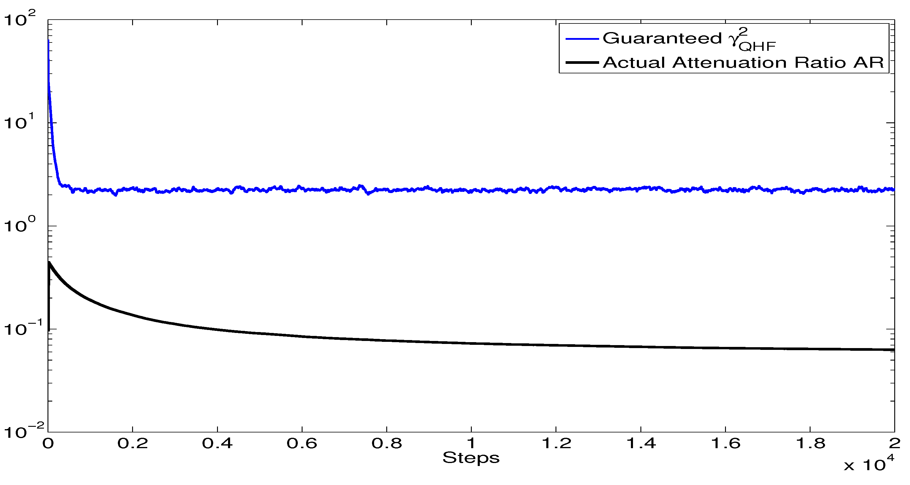
Figure 2.
Time histories of the MC-mean of the Attenuation Ratios for various initial quaternion estimates. 50 MC runs. .
Figure 2.
Time histories of the MC-mean of the Attenuation Ratios for various initial quaternion estimates. 50 MC runs. .
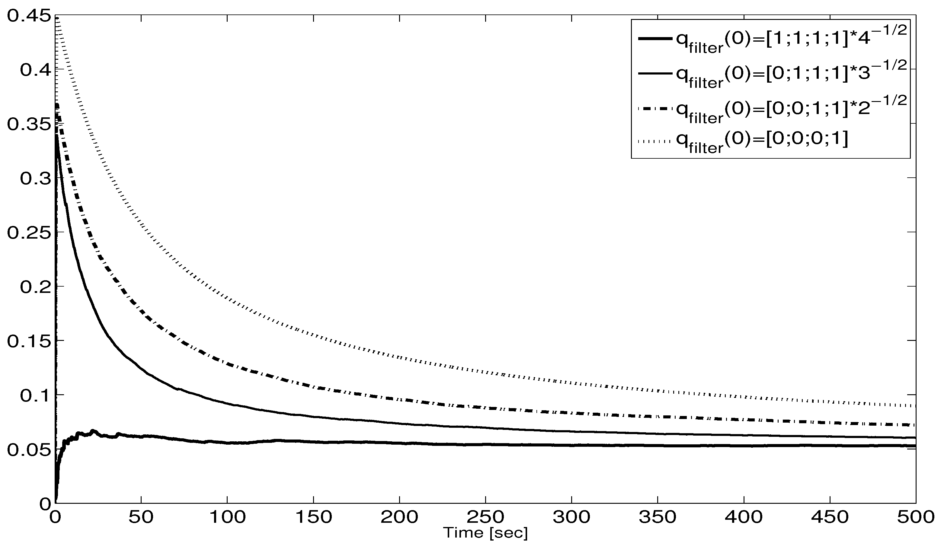
Figure 3.
Time histories of the MC-mean of the Attenuation Ratios for various initial matrix . 50 MC runs. .
Figure 3.
Time histories of the MC-mean of the Attenuation Ratios for various initial matrix . 50 MC runs. .
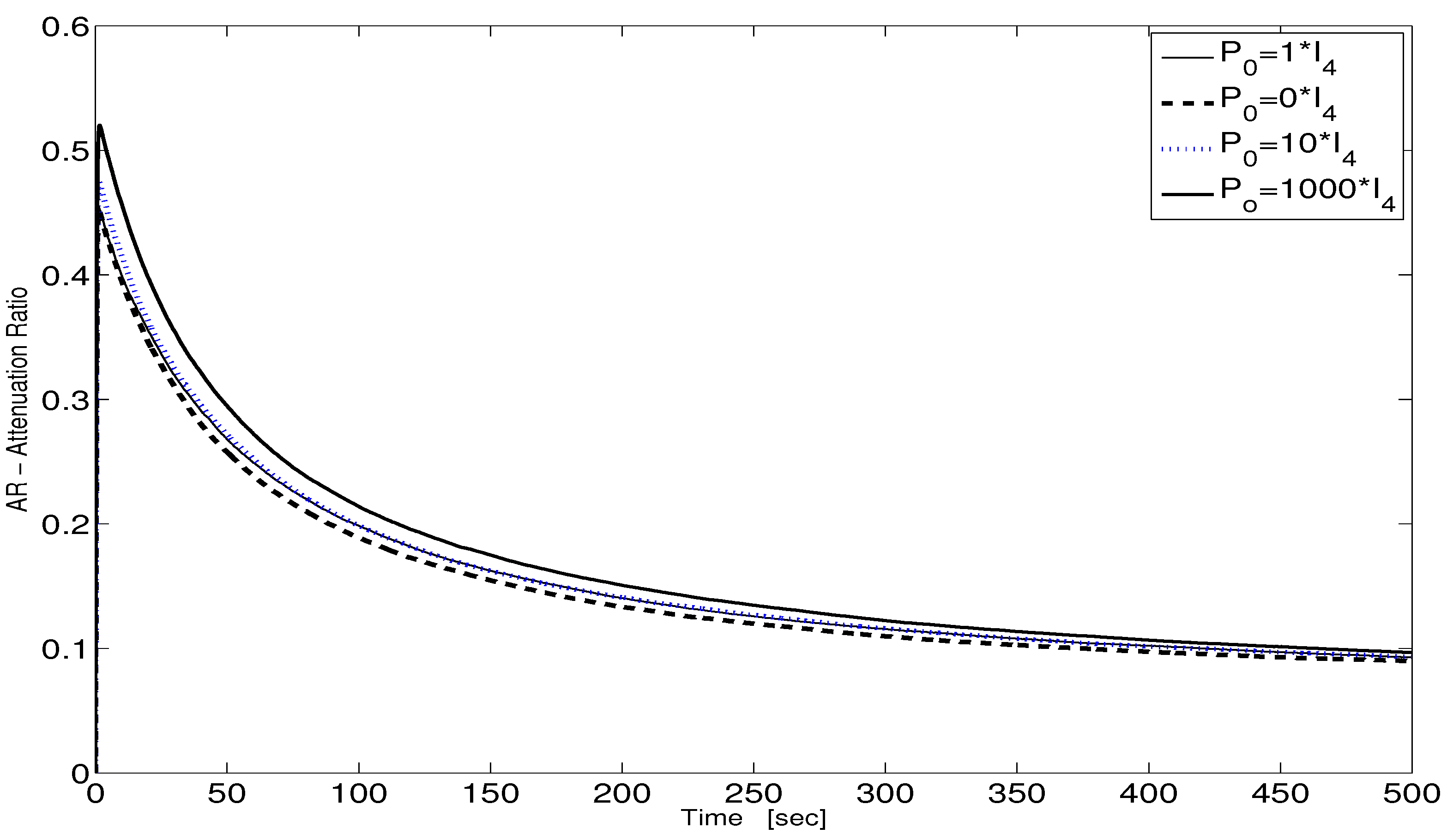
Figure 4.
Time histories of the quaternion estimation error MC-means (blue) and MC-standard deviations (red). 50 MC runs. .
Figure 4.
Time histories of the quaternion estimation error MC-means (blue) and MC-standard deviations (red). 50 MC runs. .
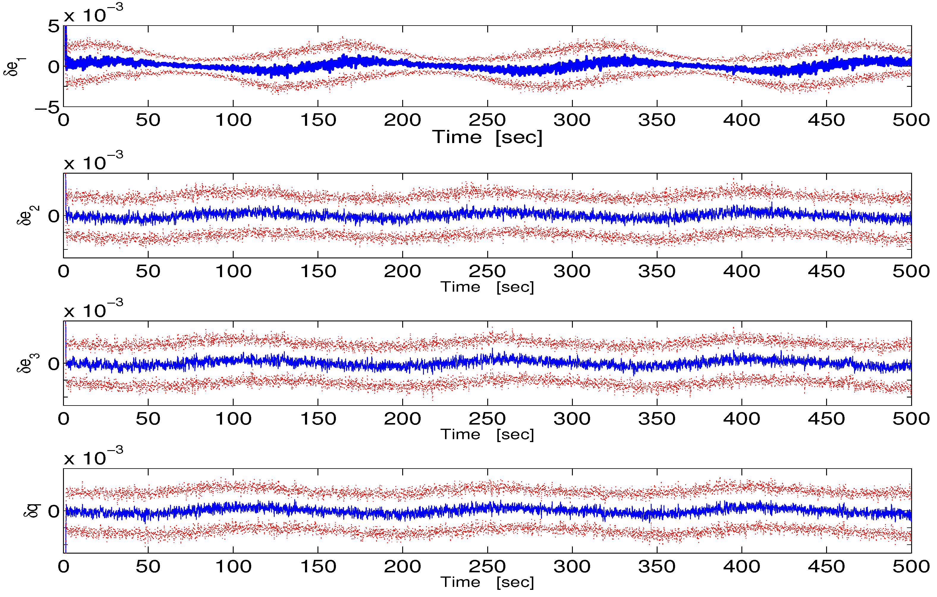
Figure 5.
Time histories of the angular estimation error MC-mean (blue) and of the ± MC- envelope (red). 50 MC runs. .
Figure 5.
Time histories of the angular estimation error MC-mean (blue) and of the ± MC- envelope (red). 50 MC runs. .
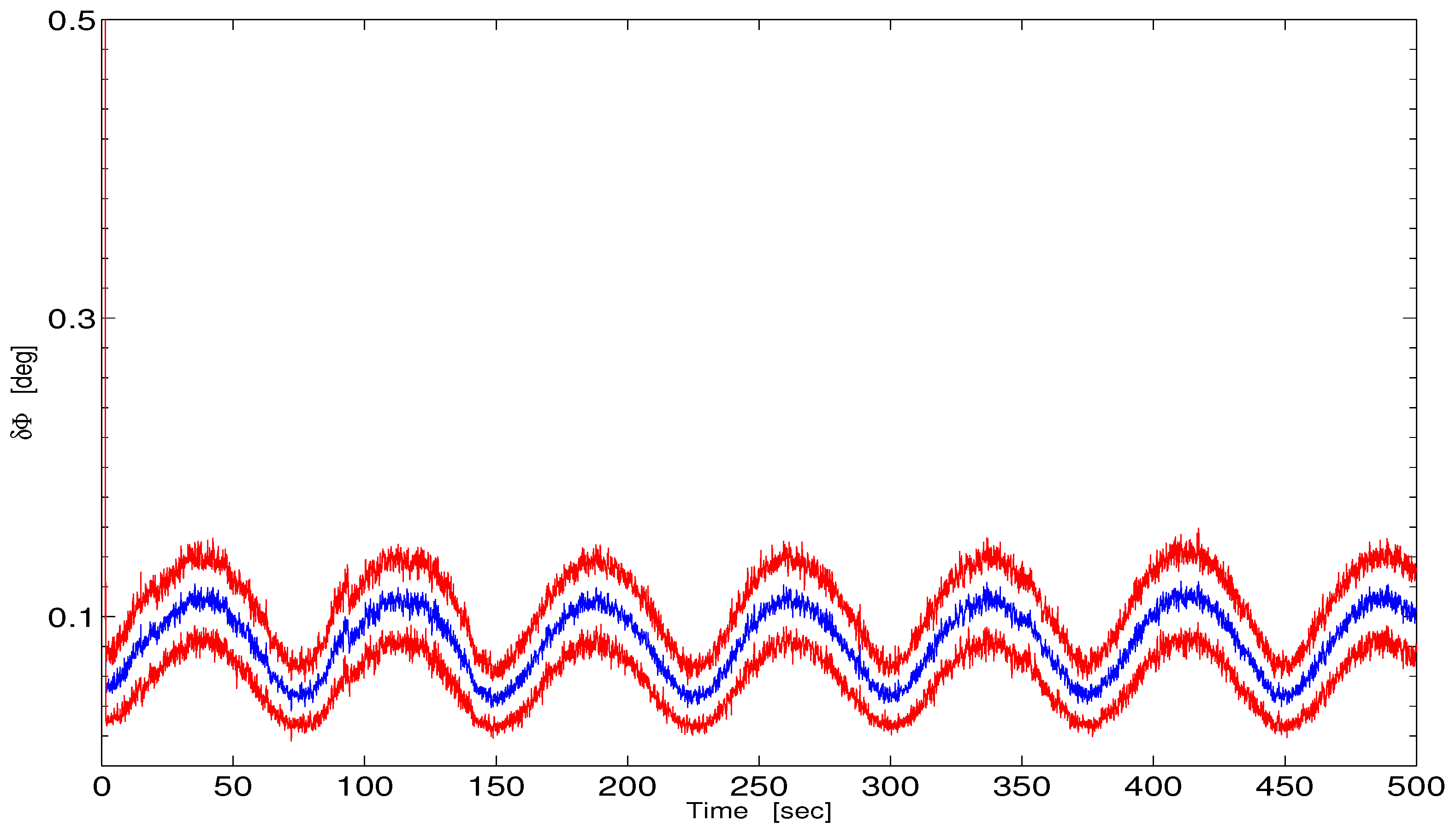
Figure 6.
Time histories of the MC-means of the quaternion estimation errors in QHF (dashed blue) and in unmatched MEKF (full red). Case A. 50 MC runs. .
Figure 6.
Time histories of the MC-means of the quaternion estimation errors in QHF (dashed blue) and in unmatched MEKF (full red). Case A. 50 MC runs. .
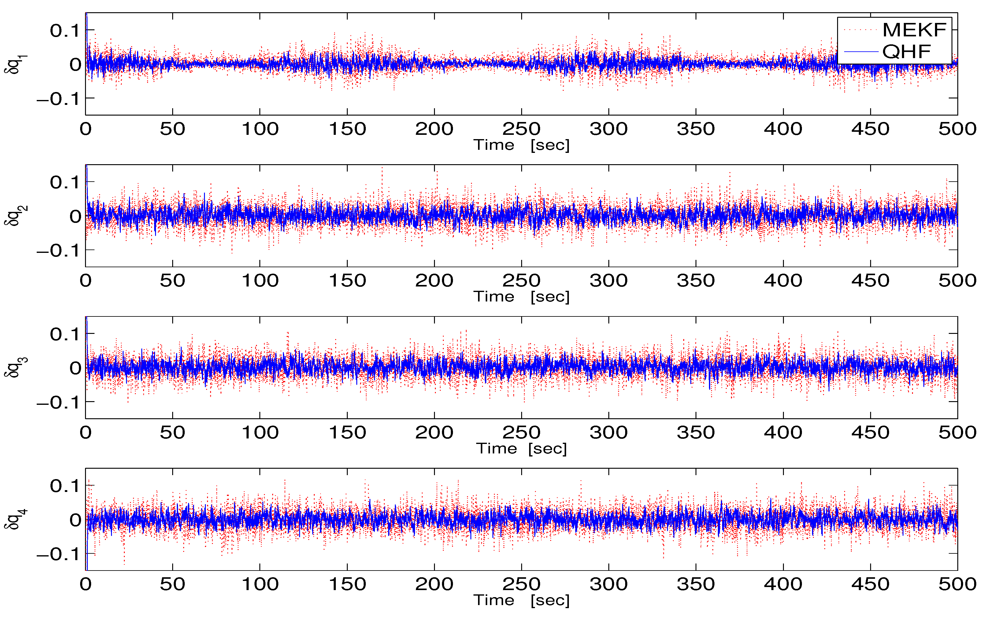
Figure 7.
Time histories of the MC-means of the quaternion estimation errors in QHF (dashed blue) and in unmatched MEKF (full red). Case B. 50 MC runs. .
Figure 7.
Time histories of the MC-means of the quaternion estimation errors in QHF (dashed blue) and in unmatched MEKF (full red). Case B. 50 MC runs. .
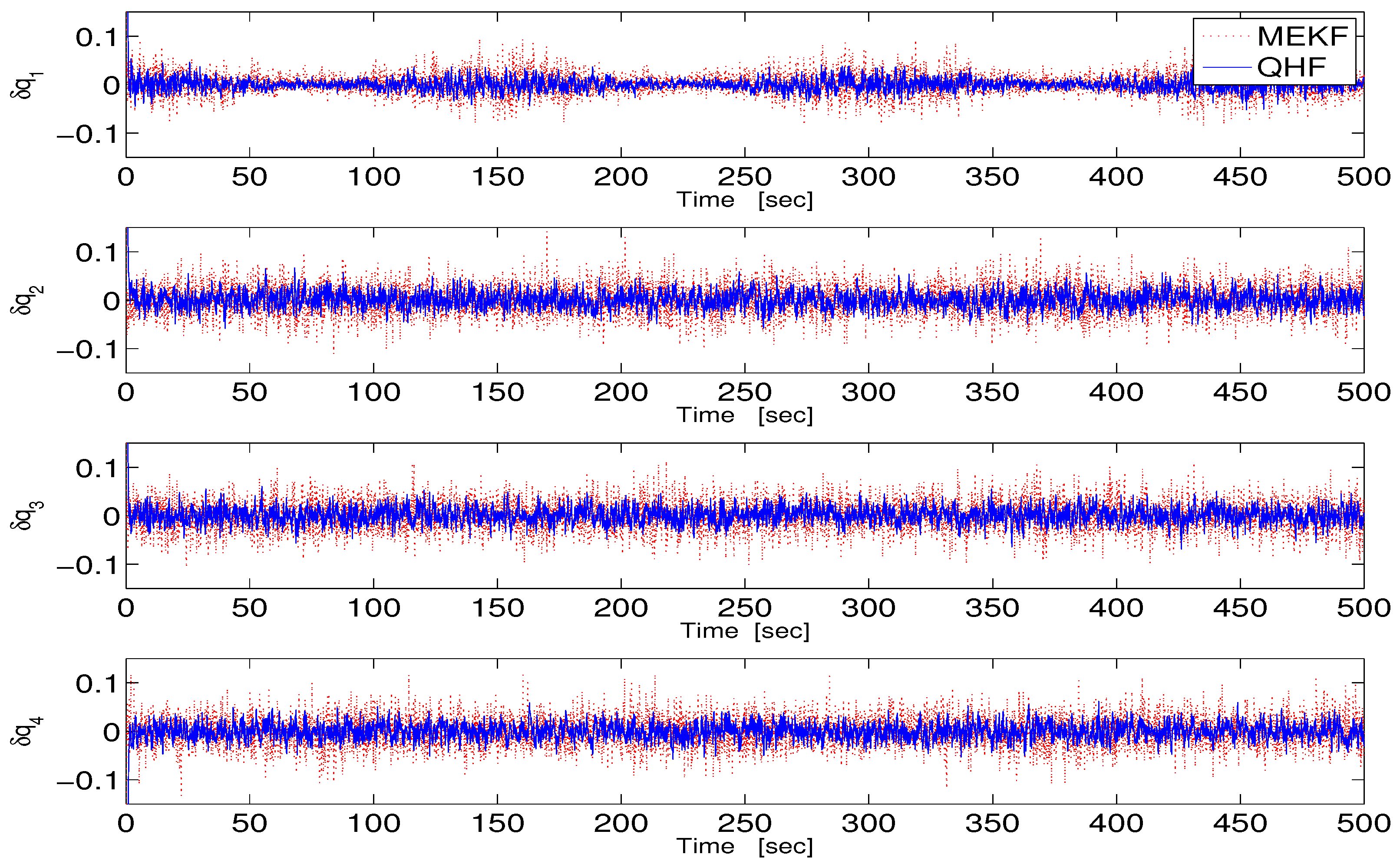

Table 1.
QHF performance. Maxima of MC-means of and of for various . 500 sec, 500 runs.
Table 2.
Ratios of the MC-means of the QHF over the QKF for various and . (Time-average of the MC-mean in the QHF in degree). 500 runs, 6000 sec.
Table 2.
Ratios of the MC-means of the QHF over the QKF for various and . (Time-average of the MC-mean in the QHF in degree). 500 runs, 6000 sec.
Table 3.
Attenuation Ratios (500 MC runs) as defined in Eq. (93) for various values of the parameters . (Value of the steady-state MC-mean of , as computed in the filter)
Table 3.
Attenuation Ratios (500 MC runs) as defined in Eq. (93) for various values of the parameters . (Value of the steady-state MC-mean of , as computed in the filter)
| 0 | ||||||
| 0 | ||||||
Table 4.
Time-averages (and time-standard deviations) of the quaternion estimation errors in the QHF (right) and in the MEKF (left) for various values of the standard deviations . Single run. Time span of 2000 seconds
Table 4.
Time-averages (and time-standard deviations) of the quaternion estimation errors in the QHF (right) and in the MEKF (left) for various values of the standard deviations . Single run. Time span of 2000 seconds
| MEKF QHF | MEKF QHF | MEKF QHF | |
Disclaimer/Publisher’s Note: The statements, opinions and data contained in all publications are solely those of the individual author(s) and contributor(s) and not of MDPI and/or the editor(s). MDPI and/or the editor(s) disclaim responsibility for any injury to people or property resulting from any ideas, methods, instructions or products referred to in the content. |
© 2024 by the authors. Licensee MDPI, Basel, Switzerland. This article is an open access article distributed under the terms and conditions of the Creative Commons Attribution (CC BY) license (http://creativecommons.org/licenses/by/4.0/).
Copyright: This open access article is published under a Creative Commons CC BY 4.0 license, which permit the free download, distribution, and reuse, provided that the author and preprint are cited in any reuse.


