System Energy Analysis and COMSOL Simulation of a Superconducting Shielding Model

Yong Gang Zheng

doi:10.20944/preprints202410.0087.v1

Submitted:

30 September 2024

Posted:

02 October 2024

Read the latest preprint version here

Abstract

This article proposes a superconducting shielding magnetic field model based on the Meissner effect of superconductors, which blocks magnetic fields. By utilizing the shielding effect of the superconductor on the magnetic field during the phase transition, the model achieves intermittent shielding of electromagnetic force, allowing the electromagnetic force to work intermittently on the moving magnet within the model during its operation. The model is analyzed on the basis of superconducting thermodynamic theory, with a focus on the electromagnetic energy of the system. It is concluded that the energy is not conserved during the operation of the model. To verify the correctness of the analysis, electromagnetic simulations and data analysis were conducted via the COMSOL electromagnetic module and Ampère's law superconducting model parameters, which yielded identical results.

Keywords:

superconducting thermodynamics

;

Meissner effect

;

electromagnetic shielding

;

energy conservation

;

COMSOL simulation

Subject:

Physical Sciences - Condensed Matter Physics

Background Technology

Thermodynamics is based on the concept of reversible phase transitions. Before the discovery of the Meissner effect, superconductors were always considered ideal conductors, with the normal state appearing when superconductivity is destroyed, resulting in resistance and heat generation from currents associated with magnetic fields. Therefore, superconducting phase transitions are viewed as nonequilibrium processes, making it impossible to understand them via thermodynamics. However, Keesom (1924), disregarding the premise of thermodynamic application, established a series of thermodynamic formulas for superconducting phase transitions, which were found to align well with a significant amount of experimental data. Gorter (1933) noted that the success of these early thermodynamic treatments strongly suggests that superconducting phase transitions should be reversible[1].

The discovery of the Meissner effect revealed that the disappearance of supercurrents in superconductors does not involve any irreversible processes. Gorter and Casimir (1934) noted that the thermodynamic treatment of superconducting phase transitions is entirely similar to that of other phase transitions, confirming the correctness of the early thermodynamic approach, and they proposed the two-fluid model[1].

The two-fluid model explains that the formation of superfluid electrons (later known as Cooper pairs) is due to the system's tendency toward the state of lowest free energy, aligning with the thermodynamic principle of minimizing free energy. The subsequent BCS theory provided a microscopic quantum explanation for Cooper pairs, describing them as pairs of electrons that condense into a lower energy state, further verifying the thermodynamic driving force behind superconductivity.

In 1935, the London brothers expanded on the two-fluid theory and, on the basis of the hypothesis of superconducting electrons and classical Maxwell equations of electromagnetism, derived the London equations. These equations demonstrate that superconducting electrons form superconducting currents in magnetic fields, which generate opposing magnetic fields that cancel out external magnetic fields. They noted that the formation and disappearance of superconducting currents are lossless, providing a strong explanation for the Meissner effect. Later, the BCS theory explained the Meissner effect on a microscopic level through the lossless motion of Cooper pairs. The London equations and BCS theory confirmed that the Meissner effect in superconductors under a magnetic field occurs without generating heat or energy loss. Conversely, when the magnetic field is removed, the disappearance of the superconducting current also occurs without energy loss. Conversely, when the magnetic field is removed, the disappearance of the superconducting current also occurs without energy loss. Under the influence of a varying magnetic field, the supermagnetic field in the Meissner state has a completely reversible transformation among the electromagnetic energy flowing into the supermagnetic field, the internal magnetic field energy, and the kinetic energy of superconducting electrons. There are no losses within the supermagnetic field[2].

Superconducting shielding is a physical function formed by the Meissner effect in superconductors. In a magnetic field, the superconductor in the superconducting state generates superconducting currents in the thin layer on its outer surface (with a thickness of 10^-2 to 10^-1 micrometers) [1,4,5], creating an opposing magnetic field that expels the internal magnetic flux (magnetic field lines), resulting in zero magnetic flux within the superconductor [1,3,4,5], effectively achieving magnetic field isolation. As shown in Figure 1, the superconductor isolates the magnetic field, thereby altering the distribution and pathways of the original magnetic field.

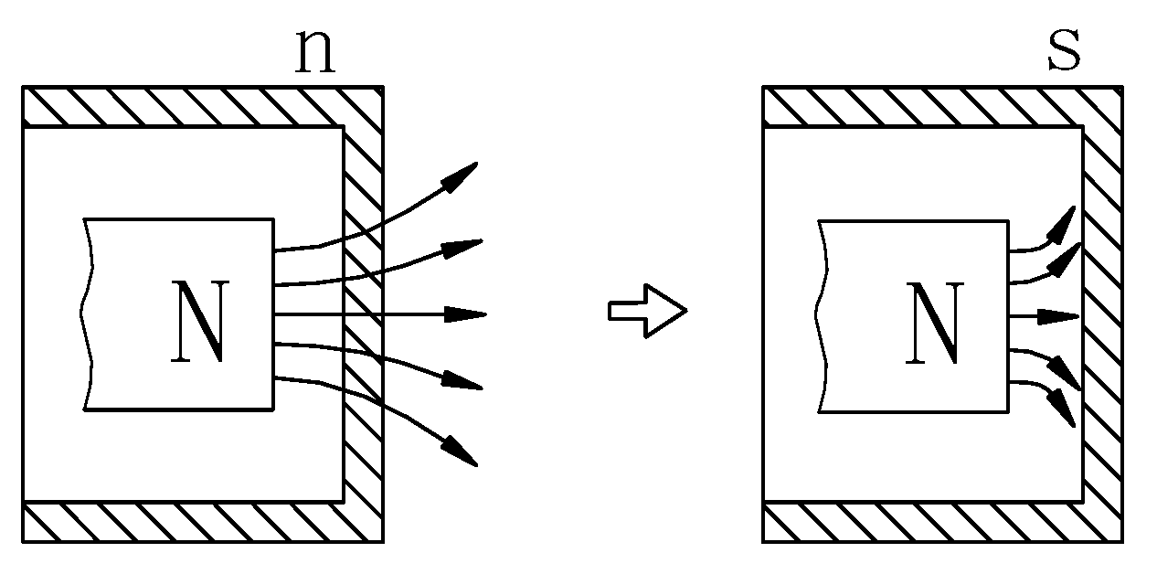
Figure 3. The magnetic field distribution generated by a real magnetic field around a superconductor.

Thermodynamic Analysis of a Superconducting Magnetic Shielding Model

First, let us introduce the thermodynamic Gibbs free energy formula[1,6]:

A superconductor in a magnetic field HHH, as shown in the second step of Figure 2, becomes magnetized in the superconducting state. The superconductor works under the influence of an external magnetic field, producing an opposing magnetic moment MMM and a superconducting current. The amount of work done is

d W = μ_{0} H d M

, where μ₀ is the permeability of free space.

The differential form of the Gibbs free energy in the presence of a magnetic field is as follows:

d G = d U - T d S - S d T + p d V + V d p - μ_{0} H d M - μ_{0} M d H

(1)

In this equation, the symbols represent the volume V, entropy SSS, pressure P, temperature T, magnetic field strength HHH, and magnetic moment M.

The Gibbs free energy in the absence of a magnetic field is as follows:

G = U - T S + P V

(2)

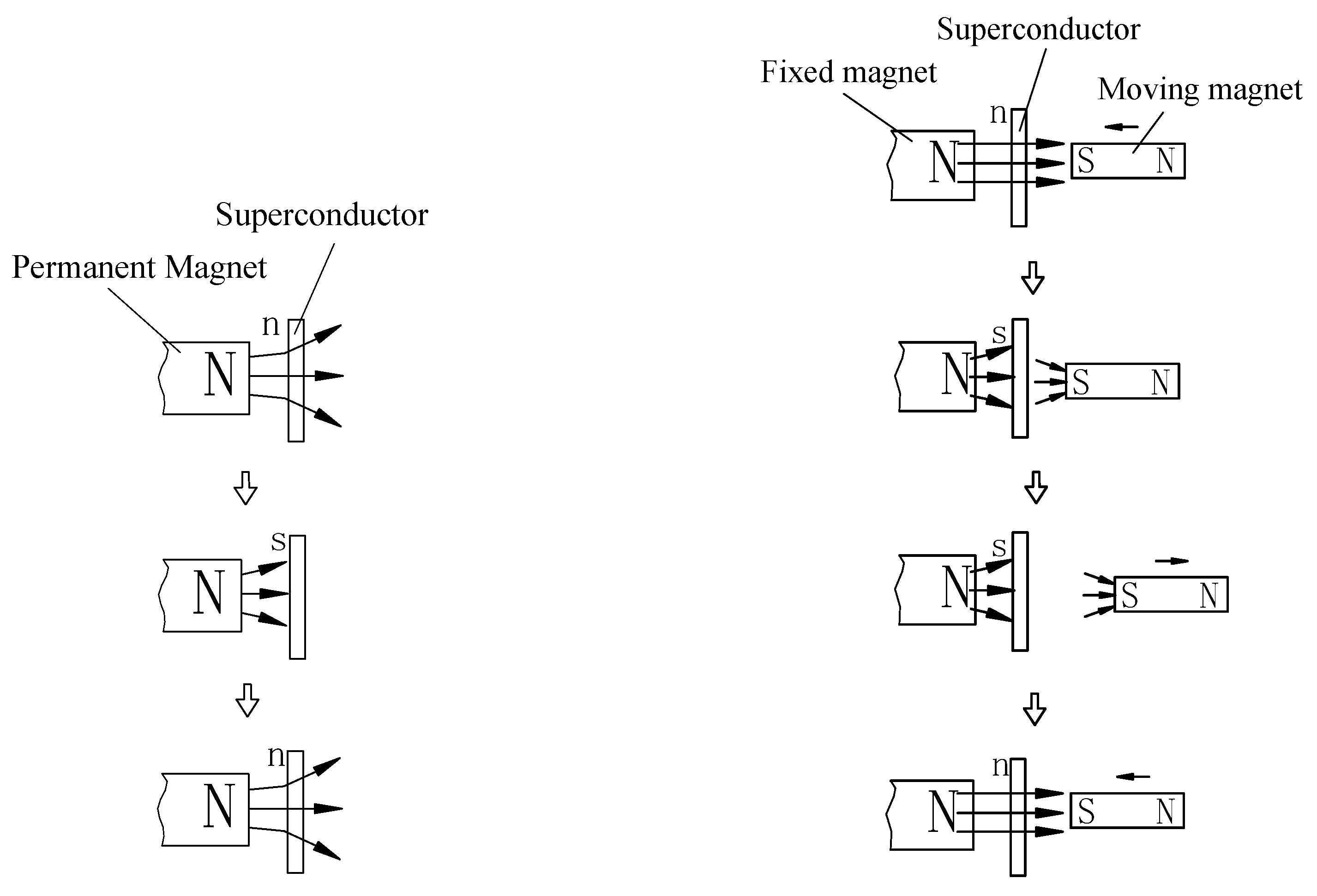
Figure 2. Basic Model.

Figure 3: Superconducting phase transition model with an added moving magnet

Note: In the figures, "s" represents the superconducting state, "n" represents the normal state, and the arrows indicate the direction of displacement.

The model in this paper, as shown in Figure 3, is similar in form to the basic superconducting thermodynamic model depicted in Figure 2. The difference is the addition of a moving magnet, which introduces a variable magnetic field. The model represents a dynamic cyclic process in which the superconductor undergoes phase transitions from the normal state to the superconducting state and then returns to the normal state.

The specific structure of the model consists of a fixed permanent magnet (referred to as the "fixed magnet") and a movable permanent magnet (referred to as the "moving magnet") placed on either side of a disc-shaped superconductor. The detailed motion of the model follows this sequence:

The superconductor starts in the normal state, with the moving magnet positioned away from the superconductor;
The moving magnet approaches the superconductor, At this time, the superconductor in the normal state behaves as a paramagnetic material, and when a moving magnet approaches, it is considered to have no effect on the superconductor[1,7]; Cooling induces a phase transition in the superconductor to the superconducting state, at which point the superconductor shields the fixed magnetic field;
The moving magnet moves away from the superconductor;
Heating causes the superconductor to return to the normal state.

The above steps complete one cycle.

Since the model presented in this paper involves a cyclic process, where superconductors transition from the normal state to the superconducting state and then revert back to the normal state, according to the thermodynamic theory of superconductivity, all the parameters, including electromagnetic energy, are reversible for superconductors that return to their original state. Therefore, any thermodynamic effects on the superconductors themselves can be offset and disregarded during the model's thermodynamic analysis. However, within this model, there is a moving magnet that, during operation, will be electromagnetically influenced by the diamagnetic field of the superconductor. Therefore, we need to reanalyze the electromagnetic energy changes between the components of the model while disregarding other parameters, such as V, S, P, and T.

According to equations (1) and (2), in the presence of a magnetic field, two additional terms are included in the system’s free energy:

μ_{0} H d M + μ_{0} M d H

. These two terms represent the work done by the external magnetic field HHH during the phase transition of the superconductor and the response of the superconductor's opposing magnetic field to changes in the external magnetic field. In fact, the first term corresponds to the work done by the magnetic field on the superconductor, generating the opposing magnetic field, whereas the second term represents the work (or potential energy) performed by the opposing magnetic field on the external field.

The thermodynamic analysis of the model in this paper considers not only the changes in the thermodynamic parameters of the superconductor but also those of the two permanent magnets. A comprehensive analysis of the three components is necessary to achieve a complete thermodynamic understanding of the model.

Next, we analyze only the changes in the thermodynamic parameters of the system caused by the external magnetic field.

Equivalent Analysis by Changing the Position of the Moving Magnet

One way to analyze the system is shown in Figure 4, where the moving magnet and the fixed magnet are placed on the same side of the superconductor at an equal distance relative to the original position. According to the superposition principle, the combined magnetic field strength of the two permanent magnets remains unchanged, and the effect on the superconductor is equivalent. The moving magnet also undergoes reciprocating motion, but in this case, over one full cycle, the work done by the fixed magnet on the moving magnet is zero. This is because this arrangement does not utilize the magnetic shielding function of the superconductor. When the moving magnet moves away, it is still subjected to the opposing electromagnetic force of the fixed magnet, and the total work done by the fixed magnet on the moving magnet before and after is zero. Therefore, the energy of the entire model is conserved.

However, in the case of Figure 3, owing to the effect of superconducting shielding, the total work done by the fixed magnet on the moving magnet before and after is greater than zero. As a result, in the model shown in Figure 3, energy is not conserved during cyclic operation, and the system gains energy.

2.: Overall Analysis Based on the Meissner Effect

The new model, which includes a moving magnet, is essentially a variation of the basic Meissner effect model. The external magnetic field acting on the superconductor is provided by two permanent magnets. According to the principle of superposition, this can be considered a combined external magnetic field, as shown in the shaded part inside the dashed box in Figure 5. As the moving magnet moves away, the magnetic field decreases, which still conforms to the Meissner effect. As the external magnetic field decreases, the opposing magnetic field of the superconductor also decreases accordingly.

For the entire model, the superconductor and the two permanent magnets exchange energy due to electromagnetic interactions, and their mutual energy influences are conserved overall. The only remaining factor is the electromagnetic work done by the fixed magnet on the moving magnet. Since this work is not zero over one complete cycle of the model, the total energy of the system is not conserved.

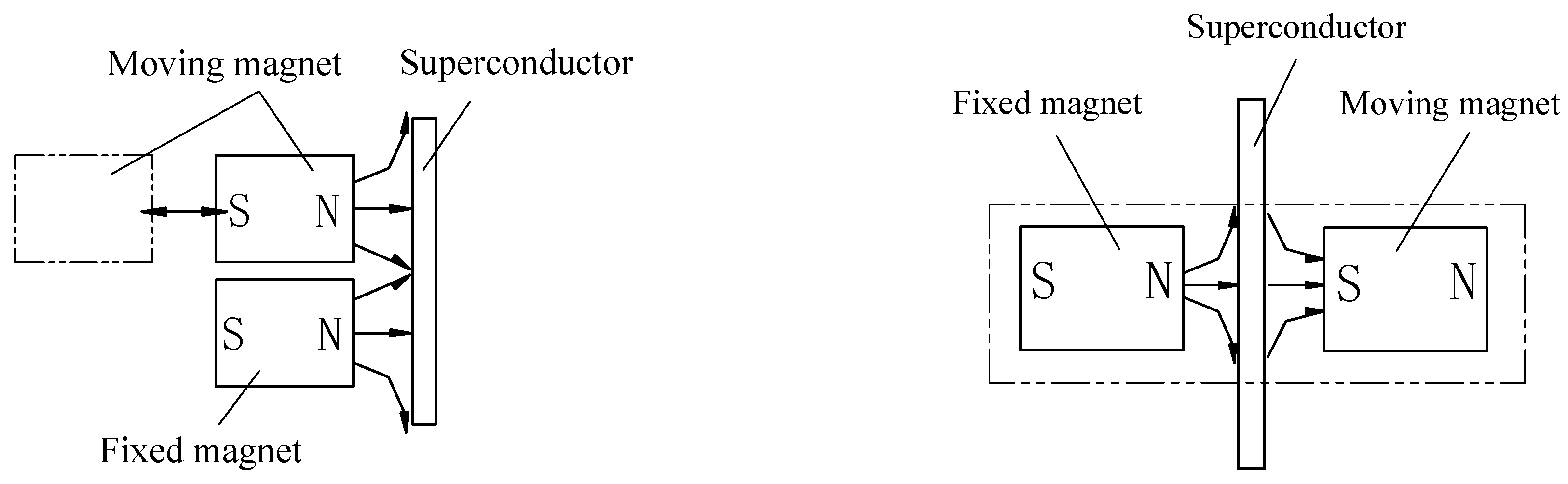
Figure 4. Schematic diagram of changing the position of the moving magnet.

Figure 5. Schematic diagram of the overall analysis.

3.: Comparative Group Analysis of the Basic Model

Let us analyze the model from another perspective. Since the energy influences are mutual, we can group the three objects in the model into pairs and analyze them separately. Finally, by subtracting the two energy-conserving basic models from the new model, the remaining interaction between the two permanent magnets becomes straightforward to analyze, as shown in Figure 6.

According to superconducting thermodynamics, Figure 6-a and 6-b each represent a complete cycle on the basis of the original model's actions, and their total energy is conserved. By subtracting the interactions between the two permanent magnets and the superconductor (as shown in Figure 6-a and 6-b) from the model, we are left with only the interaction between the fixed magnet and the moving magnet, as depicted in Figure 6-c.

In Figure 6-c, following the original model's actions, the moving magnet approaches the fixed magnet and experiences positive work due to the magnetic force. As it moves away, the magnetic field of the fixed magnet is shielded by the superconductor, so the electromagnetic force no longer acts on the moving magnet, and no electromagnetic work is performed on it.

In total, the analysis of Figure 6-c shows that positive work is generated during the model's operation. Since the subtracted components are energy-conserving, in one complete cycle of the model, positive work is generated, and thus, the system's energy is not conserved.

The above analysis, which uses several methods from different perspectives, consistently demonstrates that the energy of the model is not conserved. Furthermore, the remaining work from each analysis is the same, which is the electromagnetic work done by the fixed magnet on the moving magnet. To further prove whether there is a change in the magnetic force between the two magnets before and after being shielded by the superconductor, COMSOL simulations are used to verify the accuracy of the analysis.

4.

Analysis of the Three Objects

a)

For the superconductor:

1): In the normal state, the superconductor can be considered unaffected by the magnetic fields of the two permanent magnets.
2): When it enters the superconducting state, it is subject to the magnetic fields of the two permanent magnets, and each generates a corresponding opposing magnetic field. Here, we assume that the total work of the combined magnetic forces is $μ_{0} H d M$ .
3): As the moving magnet moves away, the opposing magnetic field works on the moving magnet. If the moving magnet moves far enough away, the superconductor is no longer influenced by the magnetic field of the moving magnet. In accordance with the Meissner effect, the opposing magnetic field generated by the superconductor due to the moving magnet disappears, resulting in work on the moving magnet.
4): However, at this point, the superconductor is still influenced by the opposing magnetic field generated by the fixed magnet.
5): When the superconductor returns to the normal state, the opposing magnetic field generated by the fixed magnet disappears, along with its capacity to perform work.
6): This step completes one phase transition cycle of the superconductor. At this point, the energy of the superconductor has returned to its original state, ensuring energy conservation.

b) For the fixed magnet, during the superconducting phase transition, the fixed magnet works on the superconductor, causing it to generate an opposing magnetic field. When the superconductor returns to the normal state, the fixed magnet recovers the work done by the superconductor. Thus, the energy of the fixed magnet remains unchanged throughout the cycle.

c)

For the moving magnet (as shown in Figure 3):

1): As the moving magnet approaches, it is subjected to the magnetic force of the fixed magnet and receives positive work[8,9].
2): When it moves away, owing to the shielding effect of the superconductor, the magnetic field of the fixed magnet is blocked, and the fixed magnet no longer exerts a magnetic force on the moving magnet or performs work on it.
3): As the moving magnet moves away, the opposing magnetic field of the superconductor performs electromagnetic work on the moving magnet. However, this work has already been discussed in the analysis of the superconductor and will be canceled out in the superconductor's energy balance, so it is not considered here.

On the basis of the above steps, the moving magnet ultimately retains the electromagnetic work done by the fixed magnet on it.

Through separate analysis of the three objects in the model, it can be concluded that during one cycle, the energy of the superconductor and the fixed magnet is conserved, whereas the moving magnet gains a net amount of work. Therefore, the system's total energy is not conserved and increases. To further confirm the correctness of these results, we analyze the system from different perspectives.

Electromagnetic simulation analysis via COMSOL

Software Adaptation Selection

COMSOL is one of the best software tools available for analyzing physical theories, offering comprehensive, rigorous, and highly reliable internal physical formulas, especially with its well-developed logical functions for electromagnetism. Therefore, COMSOL is used in this work to perform electromagnetic and thermodynamic analyses of the model.

For this specific model, the AC/DC module in COMSOL, which is suitable for electromagnetic field analysis, is applied. The parameters are set according to the characteristics of the superconductor's Meissner effect, including the magnetic permeability, electrical conductivity, and dielectric constant, to simulate the model.

2.: Model Movement Process

As shown in Figure 8, the movement process of the model is as follows:

a): A cylindrical fixed magnet is placed inside a cylindrical superconductor, which is in the normal state, with the moving magnet positioned 52 mm away from the superconductor.
b): From 0 to 5 s, the moving magnet moves at a constant speed of 1 cm per second along the negative x-axis, approaching the superconductor. After 5 s, the moving magnet stops and is now 2 mm away from the superconductor.
c): At 5 s, the superconductor begins its phase transition to the superconducting state, and by 6 s, the phase transition is complete, with the superconductor in a fully superconducting state.
d): From 5 to 8 s, the moving magnet remains stationary.
e): At 8 s, the moving magnet starts moving again at a constant speed of 1 cm per second along the x-axis. By 13 s, the moving magnet returns to its initial position in the model.

The simulation model is built on the basis of the geometric model shown in Figure 9.

1): Parameter Settings

Owing to significant differences in the properties of various superconducting materials, it is necessary to first select a material for the superconductor in this model before setting the parameters. To simplify the analysis, this model is based on a Type I superconductor and uses the parameters of a well-known material, niobium-titanium alloy (NbTi).

The parameter settings for the superconductor model are based on superconducting theory: the magnetic flux inside the superconductor is zero, and the current experiences no resistance. In other words, when the superconductor is in the superconducting state, its relative magnetic permeability is 0, and its electrical conductivity is infinite.

The theoretical foundation follows Ampère's law, making the "magnetic fields" (mf) physics module the most suitable for simulating superconducting shielding. The "magnetic fields" module is specifically designed on the basis of Ampère's law to build electromagnetic fields. The internal equations within "magnetic fields" adhere to existing electromagnetic theory, including the London equations from superconducting theory, which are based on Maxwell's electromagnetic equations. Therefore, the use of "magnetic fields" for simulating superconducting shielding is both appropriate and correct.

For the superconductor in the superconducting state, the relative magnetic permeability is set to 0, and the electrical conductivity is set to infinity. However, in COMSOL, the relative magnetic permeability cannot be set to 0. According to superconductivity theory and the paper on superconducting shielding[1,2], for simulations, the relative magnetic permeability is typically set between 10⁻² and 10⁻⁵, and the electrical conductivity is generally set to 10⁵. In this model, the relative magnetic permeability of the superconductor is set to 10⁻⁵, and in the normal state, the superconductor is typically paramagnetic, so its relative magnetic permeability is set to 1. The superconductor in this model is assumed to be a niobium‒titanium (NbTi) alloy. In the normal state, the electrical conductivity of the superconductor has little effect on the electromagnetic properties of paramagnetic materials, so the electrical conductivity is also set to 10⁵.

The physics interface for the superconductor uses the "Ampere's law in solids" interface from COMSOL's "magnetic fields" module, with the relative magnetic permeability and electrical conductivity set according to the values mentioned above.

For the permanent magnets in the model, the parameters are set according to commonly used permanent magnetic materials in the software. Both the fixed and moving magnets are assigned the material N54 (sintered NdFeB), with the magnetic flux density modulus slightly reduced to 0.2 T. When the moving magnet is replaced with a ferromagnetic material, its relative magnetic permeability is set to 40,000. The surrounding environment is modeled using air.

4.: Simulation process

After the materials, physical fields, and interface parameters are determined, the mesh size and precision are set to ensure that the model calculations converge. Since the model is dynamic, to simplify the process and reduce the computation time, the parametric sweep function in COMSOL is used. The time cycle for the model is set to 13 seconds.

5.: Explanation of the Contour Plot

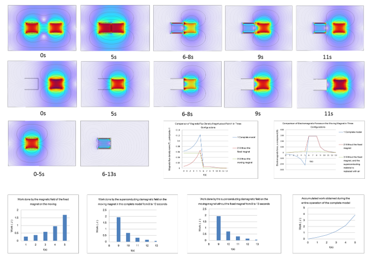
After running the model, the simulation results are shown in Figure 10, which presents electromagnetic distribution contour plots at six key time points.

The results indicate that during the movement process, from 0 to 5 s, the superconductor is in its normal state, behaving as a paramagnetic material, and thus has no effect on the magnetic fields of the two permanent magnets. Between 5 and 6 s, the model is in a transitional state, which can be considered an intermediate state of superconductivity. Since a parametric sweep was used, the intermediate state is not physically accurate (in reality, the phase transition temperature range of Type I superconductors is very narrow, as small as 10^--3). Therefore, there is no need to analyze the intermediate state.

From 6 to 13 s, the superconductor is in the superconducting state, the internal magnetic flux is expelled, and the magnetic flux inside the superconductor becomes zero. A counteracting magnetic field forms on the inner and outer surfaces of the superconductor, opposing the external magnetic field, which is consistent with superconducting theory. At this point, the superconductor not only shields the magnetic field of the fixed magnet from its interior but also generates an opposing magnetic field outside, which exerts a positive electromagnetic repulsive force in the x-direction on the moving magnet.

To facilitate observation, the moving magnet remains stationary during the period from 5--8 seconds. At 8 s, the moving magnet begins to move away from the superconductor, and the opposing magnetic field outside the superconductor starts to weaken. This behavior is fully consistent with the Meissner effect of the superconductor (excluding the pinning effect of Type II superconductors here).

The contour plots of the model during the movement process align perfectly with the theoretical analysis of the model discussed earlier.

6.: Data analysis

After completing the simulation of the full model, the first step is to verify whether the model satisfies the principle of electromagnetic superposition. Using COMSOL, simulations were performed for the combination models described in Part 3, and the results were analyzed through superposition.

From the simulation results of the three combination models, two important electromagnetic parameters are extracted for analysis:

1. The x-direction electromagnetic force is exerted on the moving magnet during the operation of the model.

2. The magnetic flux density modulus at point 1 of the model is shown in Figure 9.

By comparing the variation curves of these two parameters across the three combination models, the applicability of the superposition principle to this model is analyzed. Figure 11 and Figure 12 show the two combinations of the moving magnet and superconductor and the fixed magnet and superconductor, respectively. Figure 13 and Figure 14 display the simulation result contour plots for these two combinations.

After the model is broken down, one more combination involving the fixed magnet and moving magnet remains, which considers only the interaction between the two without involving the superconductor. This will not be discussed at this stage and will be addressed separately later.

After the simulation results are computed, the parameter curves are extracted. Figure 15 shows the magnetic flux density modulus curve at point 1 in the complete model. Figure 16 shows the magnetic flux density modulus curve at point 1 in the model without the fixed magnet. Figure 17 presents the curves from different combination models for comparison and analysis.

In Figure 17, during the 0–5 second interval, the superconductor is in the normal state, is unaffected by the magnetic field, and does not generate an opposing magnetic field. Furthermore, from 0–5 seconds, it is clear from the three curves that the sum of curves 1 and 2 equals the data of curve 3, which proves that the simulation results are consistent with the principle of electromagnetic field superposition, matching the actual behavior.

Now, let us focus on analyzing the 6–13 second segment of the curves. Between 6–8 s and 8–13 s, curves 1 and 2 almost overlap, showing that the magnetic flux density moduli for both curves are equal. This indicates that the external magnetic field of the superconductor is the same in both states, meaning that the magnetic field of the fixed magnet has been completely shielded by the superconductor. The magnetic flux density on the outer surface of the superconductor is generated entirely by the moving magnet, and the fixed magnet no longer has any influence. Curve 3, which is zero after 6 s, further confirms that the fixed magnet no longer affects the external field of the superconductor.

From a reverse perspective, the magnetic field of the moving magnet affects only the inner surface of the superconductor, whereas the fixed magnet affects only the outer surface of the superconductor. This means that the electromagnetic effects on the superconductor in the model of Figure 11, combined with the effects in the model of Figure 12, equal the total electromagnetic influence of both permanent magnets on the superconductor in the complete model shown in Figure 9.

To summarize the previous analysis, the electromagnetic influence of the permanent magnets on the superconductor in the models of Figure 11 and Figure 12, when superimposed, is entirely equivalent to the combined influence of both permanent magnets on the superconductor in the model of Figure 9.

Additionally, the overall energy in the models of Figure 11 and Figure 12 is conserved during the operation process. On the basis of the equivalent analysis, the combined electromagnetic influence between the two permanent magnets and the superconductor in the model of Figure 9 is also energy conserved.

Since the electromagnetic interaction between the two permanent magnets and the superconductor has been analyzed, let us focus on the interaction between the moving magnet and the fixed magnet during the operation of the model.

The contour plots and the curve in Figure 17 clearly show that during the 0–5 second interval, the fixed magnet exerts an attractive electromagnetic force on the moving magnet and performs positive work on it. After 6 s, as shown by curve 3, the magnetic flux density modulus of the fixed magnet outside the superconductor drops to zero, meaning that it no longer exerts any electromagnetic influence on the moving magnet. Therefore, over the entire time period, the fixed magnet performs positive work on the moving magnet.

If the two permanent magnets were not in the model, the reciprocating motion of the moving magnet would result in the fixed magnet performing alternating positive and negative work of equal magnitude on the moving magnet, resulting in zero work. However, within the model, the situation is different because of the superconductor’s magnetic shielding function, which effectively isolates the magnetic fields. The magnetic flux does not reach the opposite magnet, and thus, the magnetic force disappears. According to the model, the moving magnet experiences a magnetic force from the fixed magnet when approaching but no force when moving away.

In summary, in the complete model shown in Figure 9, the remaining effect is the positive work performed by the fixed magnet on the moving magnet during the 0–5 second interval. This indicates a change in the system’s energy, and the model generates positive work, increasing the free energy.

Next, we further analyze the model’s energy change by examining the electromagnetic force experienced by the moving magnet.

Figure 18 shows the electromagnetic force curve for the complete model, Figure 19 shows the curve for the model without the fixed magnet, and Figure 20 compares the electromagnetic force curves for the two models.

The electromagnetic force provides a more intuitive explanation of the superposition principle. After 6 s, when the superconductor shields the fixed magnet, the two curves almost overlap, indicating that the electromagnetic force on the moving magnet is nearly the same in both models. This confirms that the electromagnetic force acting on the moving magnet in the complete model at that point is entirely provided by the superconductor’s opposing magnetic field, which aligns with the previous superposition theory analysis.

Figure 19 shows that in the model without the fixed magnet, the electromagnetic force curve during the 0–5 second interval is small and gradually increases in the positive x-direction electromagnetic force. Initially, it was thought that there might be a parameter discrepancy in the superconductor settings, causing the superconductor in its normal state to exert some electromagnetic force on the moving magnet. To verify the correctness of the superconductor parameter settings, the model was modified by setting the superconductor material to air. After running the simulation and outputting the electromagnetic force curve, it was found to match exactly with the curve where the relative magnetic permeability of the superconductor in the normal state was set to 1. This demonstrates that even if an object is set as air in COMSOL, it still exerts a small electromagnetic force on the magnet. Importantly, this proves that the superconductor parameter settings in the normal state were correct. This finding also suggests that solid paramagnetic materials exert a slight electromagnetic force on permanent magnets.

The electromagnetic force analysis further confirms the correctness of the electromagnetic superposition principle in the model, supporting the accuracy of the earlier theoretical analysis.

By using the electromagnetic force curves, the work done by the electromagnetic force can be calculated through integration over the displacement variable. Since COMSOL does not directly offer the functionality to integrate electromagnetic force along the displacement direction, this paper extracts the electromagnetic force data from the model and uses EXCEL or MATLAB to perform displacement integration for each segment of the curve, obtaining the electromagnetic work for each time interval. As shown in Figure 22 to 25, excluding Figure 22, which shows the electromagnetic work of the superconductor on the moving magnet, Figure 24 displays the remaining work. Figure 25 shows the cumulative numerical results for Figure 24.

When comparing Figure 23 with Figure 22, the values are almost identical, indicating that during the 8–13 second interval, the superconductor completely shields the magnetic field of the fixed magnet, and the electromagnetic work exerted on the moving magnet is entirely provided by the opposing magnetic field of the superconductor. The fixed magnet no longer exerts any negative work on the moving magnet.

The simulation model not only confirms the correctness of the electromagnetic superposition principle but also directly calculates the remaining work generated during the model's operation.

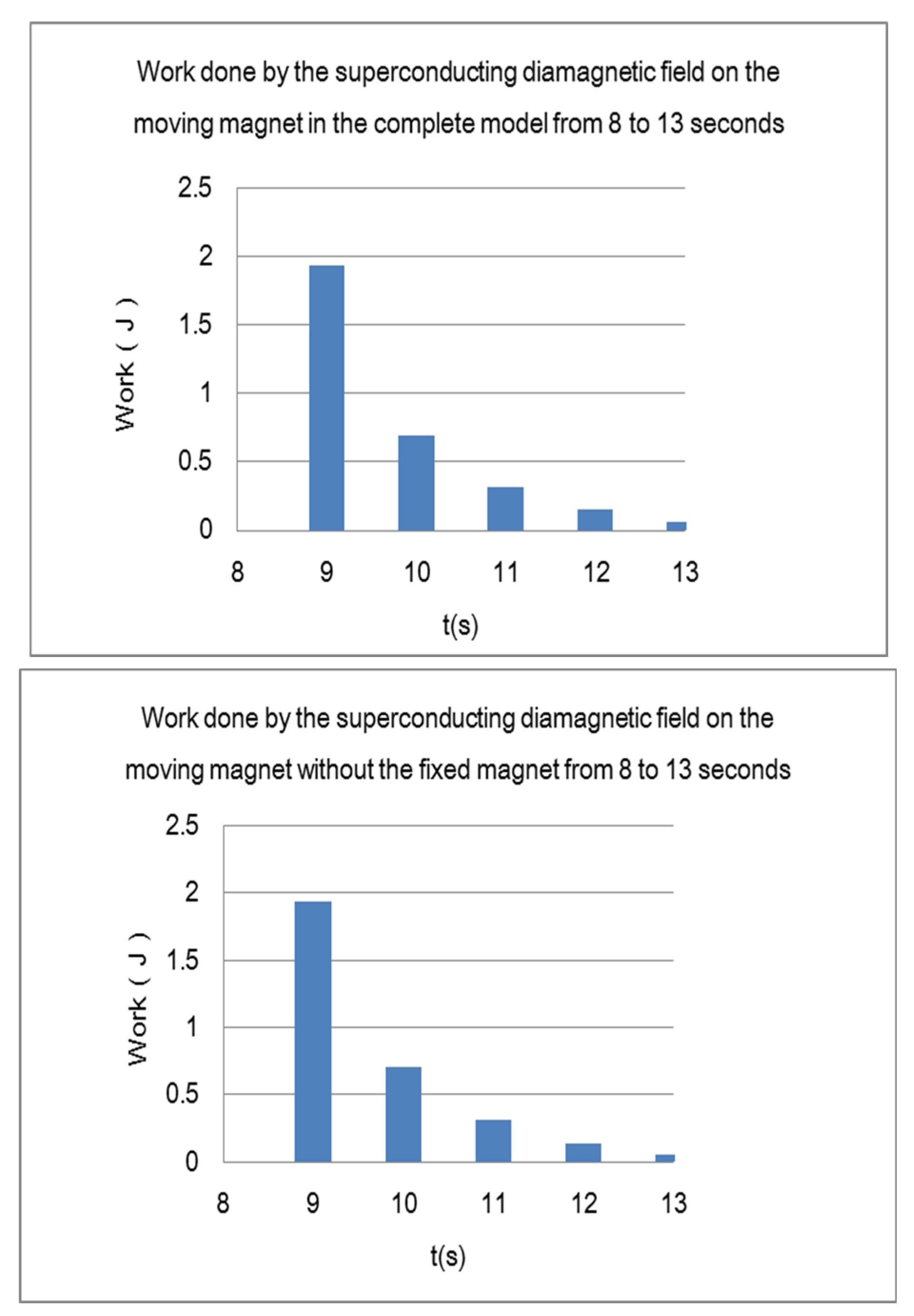
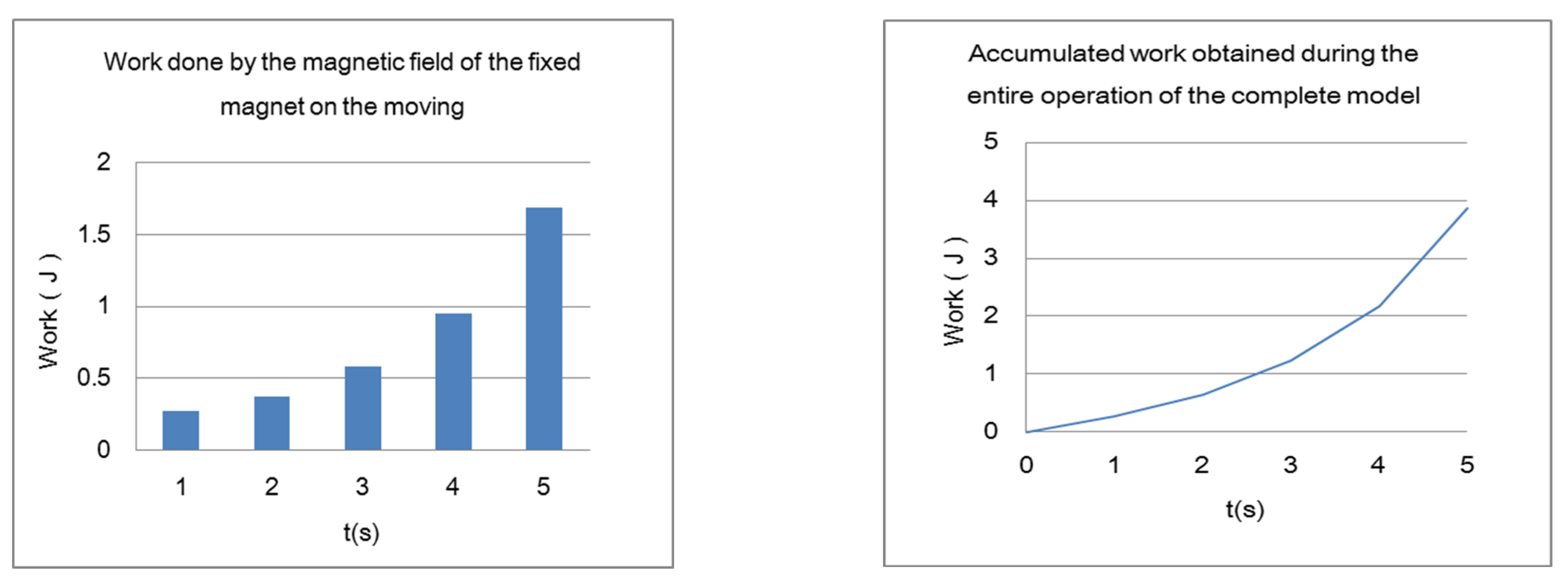
Figure 22. Electromagnetic Work on the Moving Magnet in the Complete Model During 8–13 Seconds.

Figure 23. Electromagnetic Work on the Moving Magnet Without the Fixed Magnet During 8–13 Seconds.

Figure 24. Electromagnetic Work on the Moving Magnet in the Complete Model During 0–5 Seconds.

Figure 25. Cumulative Electromagnetic Work on the Moving Magnet in the Complete Model During 0–5 Seconds.

7.: Simulation Conclusion

The simulation analysis results show that the electromagnetic interactions between the superconductor and the two permanent magnets conform to the principle of electromagnetic superposition, proving that the derivations and analysis in the second part of this paper are entirely correct. Additionally, the simulation directly calculates the positive work done by the fixed magnet on the moving magnet, indicating that the model produces positive work during operation, leading to an increase in energy. Figure 26 presents an integration of the simulation contour plots and the calculated data.

Experimental Setup

The experimental setup for model verification is shown in Figure 27. Currently, the necessary conditions for constructing the experimental setup are not available. Once the conditions for building the setup are met, experimental verification is conducted. Although the model cannot be experimentally tested at the moment, both theoretical derivations and simulation analysis have yielded completely consistent results.

Conclusion

This work, which is based on superconducting thermodynamic theory and other superconducting theories, analyzes the thermodynamic energy of the model from different perspectives and uses several different methods. The analysis revealed that the thermodynamic energy of the model system is not conserved. COMSOL simulations were used to verify this conclusion, which not only qualitatively confirmed the correctness of the theoretical analysis but also yielded the same results quantitatively. In the end, the superconducting shielding model presented in this paper does not conserve thermodynamic energy, indicating that there are situations where the first law of thermodynamics may not be applicable.

References

Zhang Yuheng. Superconducting Physics. Hefei: University of Science and Technology of China Press, 2009, pp. 31-36, 42-43.
Zhao Shangwu, Wang Haifei, Yang Xinrong, Wang Qiuliang. Electromagnetic Field and Energy Changes in Superconductors in the Meissner State under the Action of an Alternating External Magnetic Field. Journal of Low Temperature Physics, 2015, 37(1), pp. 66-69.
Liu Huan. Research on Magnetic Shielding and Magnetic Transmission Properties of Superconductor-Ferromagnetic Metamaterials. Master's Thesis. Chengdu: Southwest Jiaotong University, 2015, p. 21.
Hu Xuefeng. Simulation Study of Magnetic Shielding in Multilayer Shields Containing Superconductors. Master's Thesis. Changsha: Hunan University, 2015, pp. 1-66.
Zhang Wanying, Zhang Jiefeng, Shi Le, Liu Donghui, Hu Xuefeng, et al. Simulation Study of Magnetic Shielding Properties in Multilayer Shields Containing Superconductors. Journal of Low Temperature Physics, 2017, 39(2), pp. 16-21.
Wang Zhicheng. Thermodynamics and Statistical Physics. Beijing: Higher Education Press, 2013, pp. 68-70.
Yu Li, Hao Bailin, Chen Xiaosong. Edge Miracles: Phase Transitions and Critical Phenomena. Beijing: Science Press, 2016, pp. 28-29.
Hu Youqiu, Cheng Fuzhen. Electromagnetism and Electrodynamics [Volume 2]. Beijing: Science Press, 2014, pp. 87-88.
Guo Shuohong. Electrodynamics. Beijing: Higher Education Press, 2008, p. 78.

Figure 6. The model is divided into three combination diagrams.

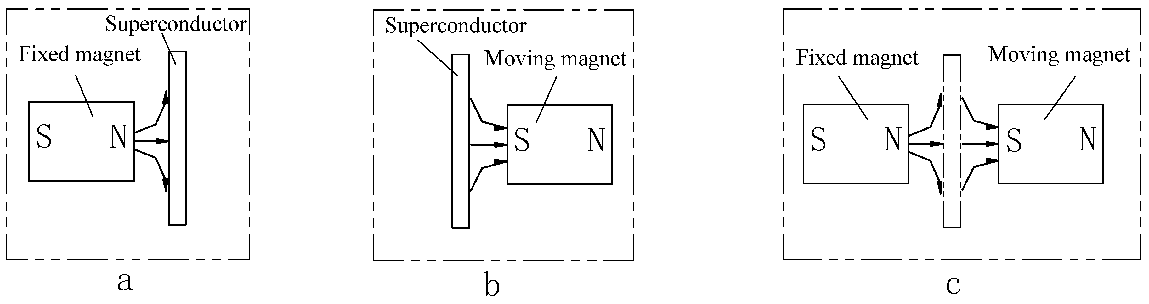
Figure 7. Schematic diagram of the group analysis process.

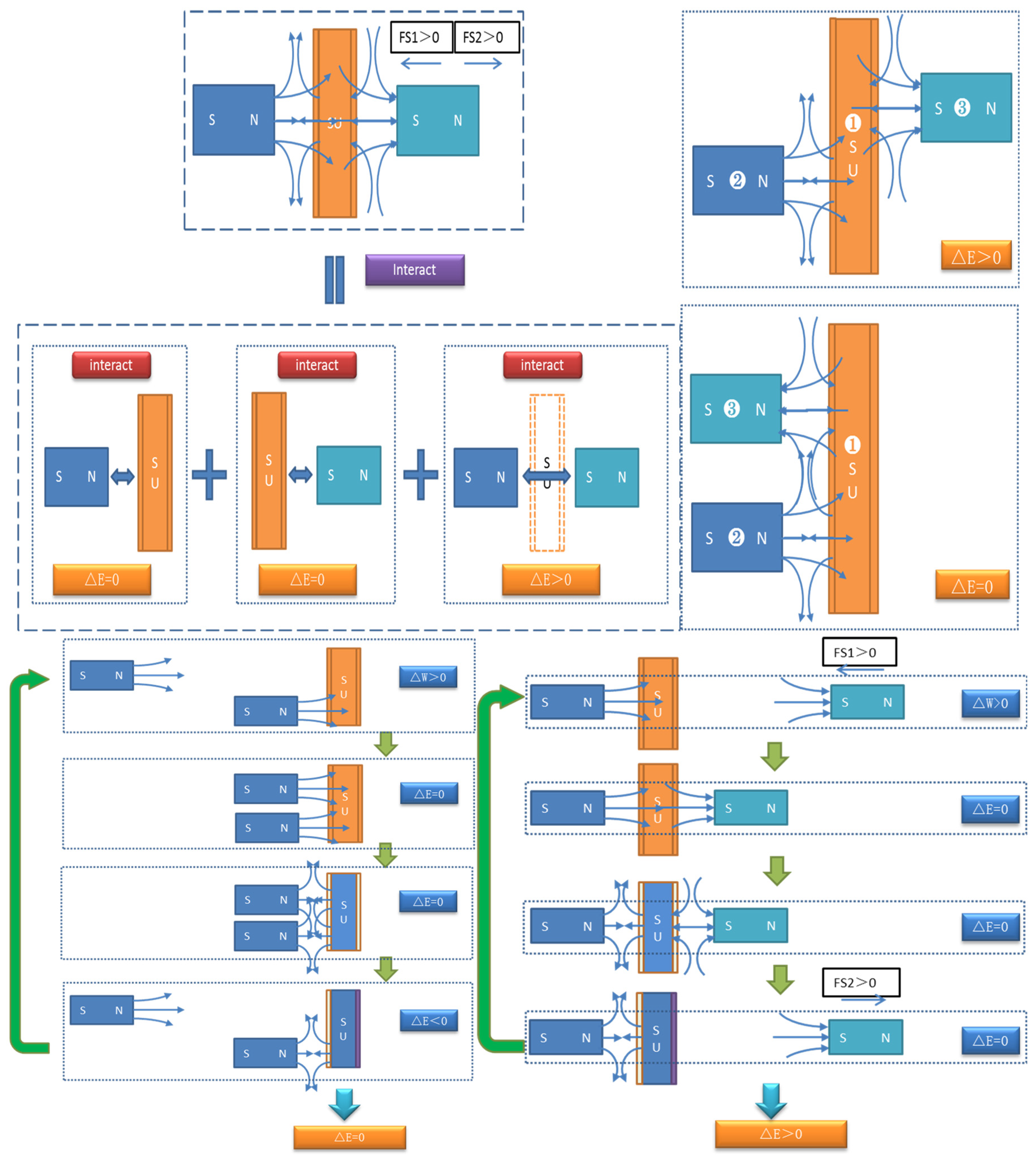
Figure 8. Geometric Model.

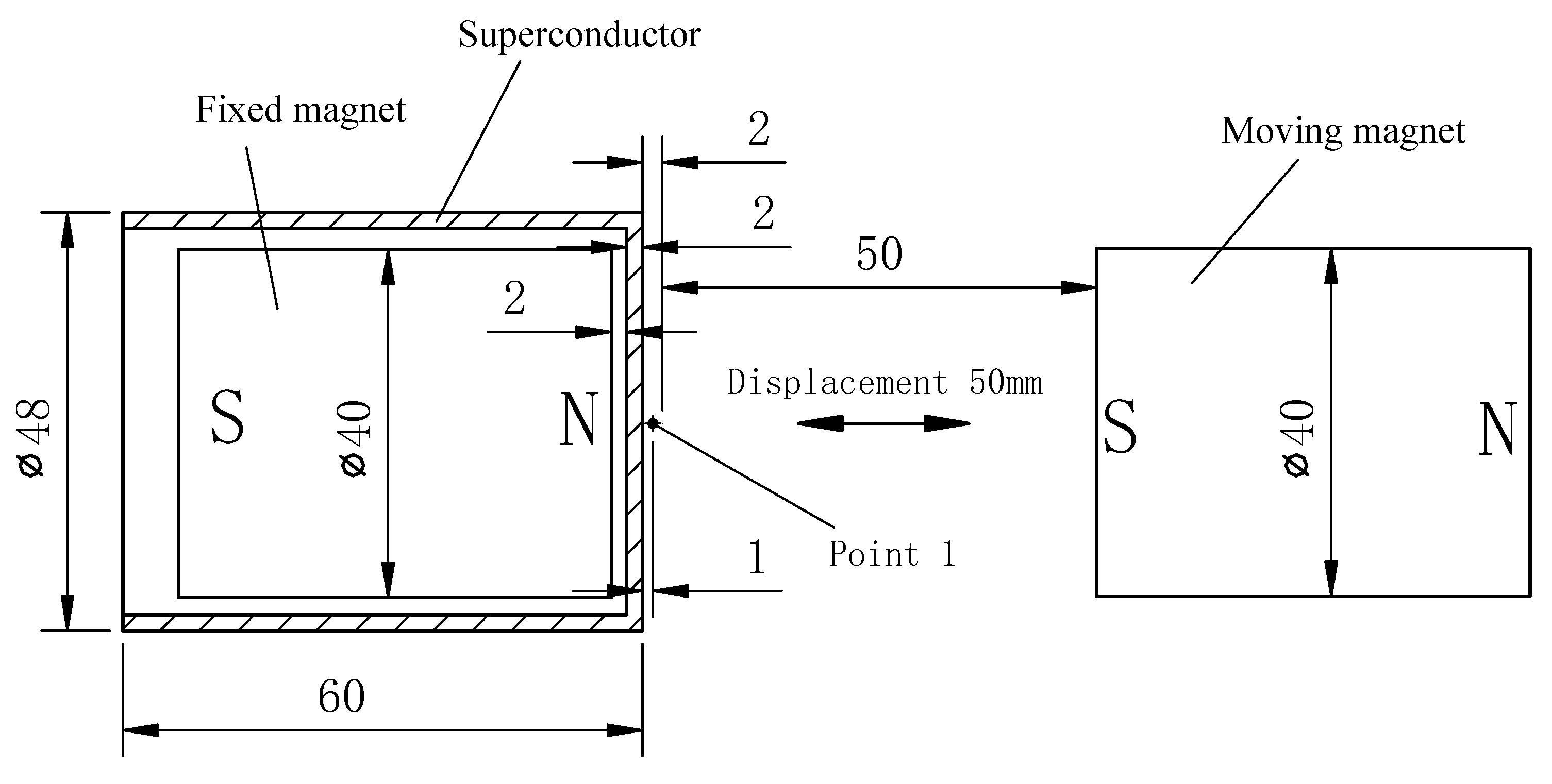
Figure 9. Simulation Model.

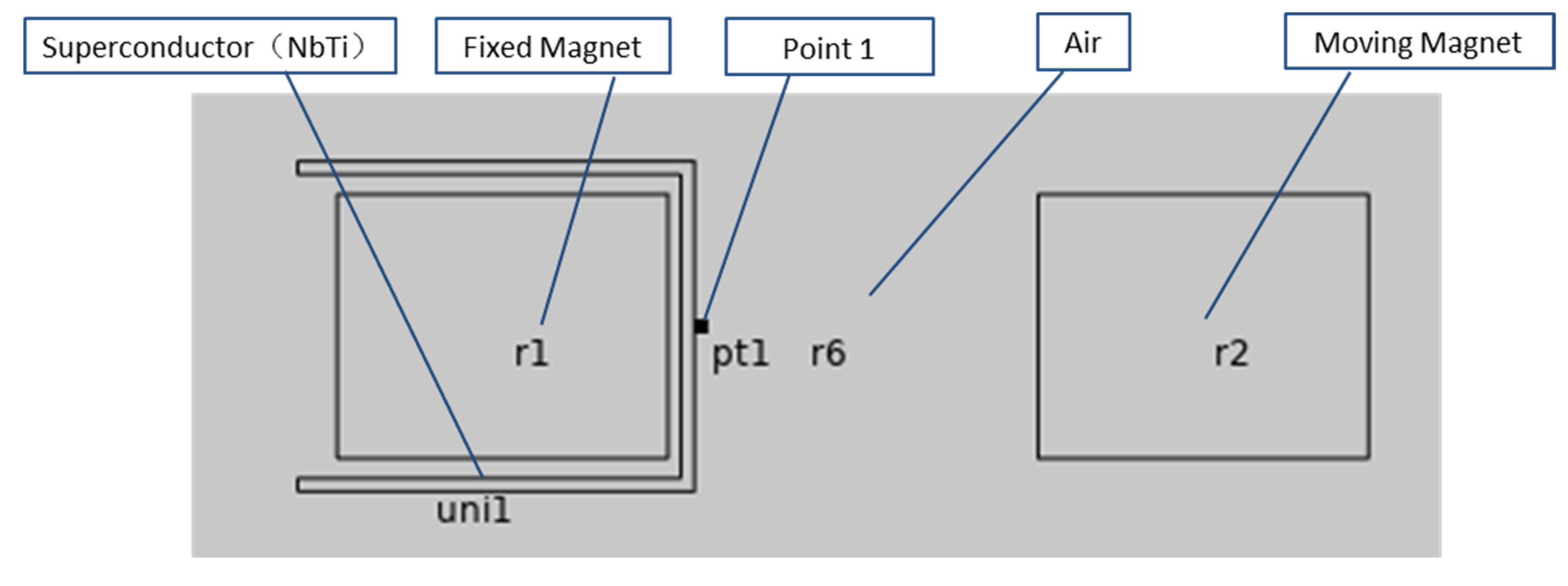
Figure 10. Electromagnetic field distribution at various time points in the model.

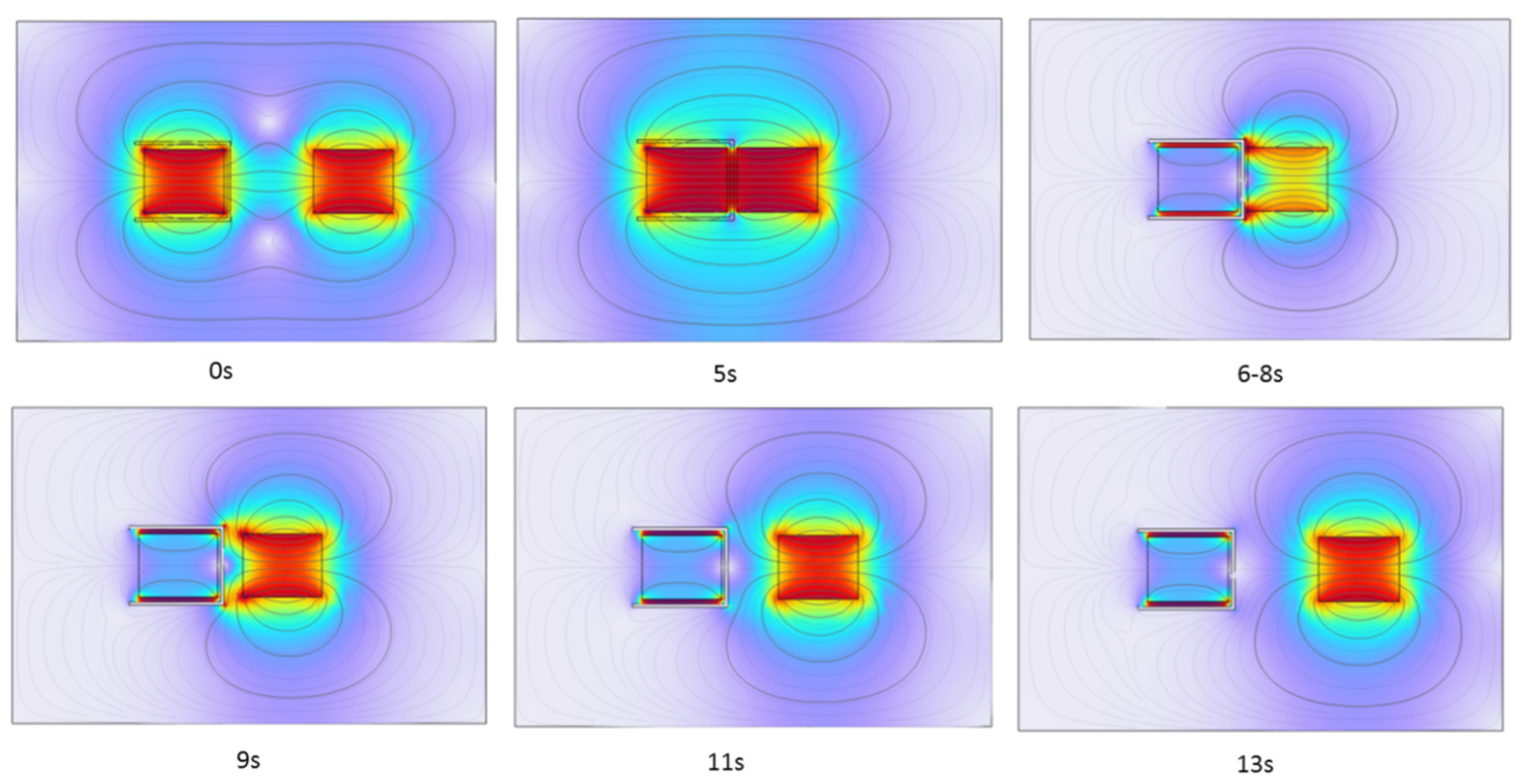
Figure 11. Model Without Fixed Magnet

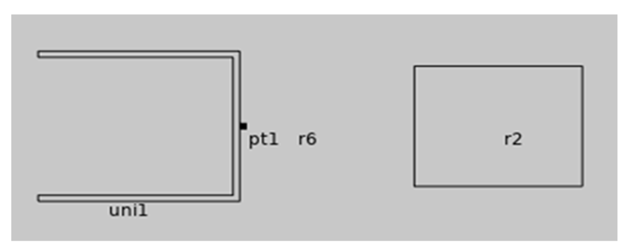
Figure 12. Model Without Moving Magnet.

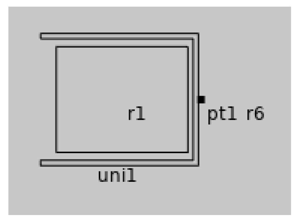
Figure 13. Electromagnetic field distribution at various time points in the model without a fixed magnet.

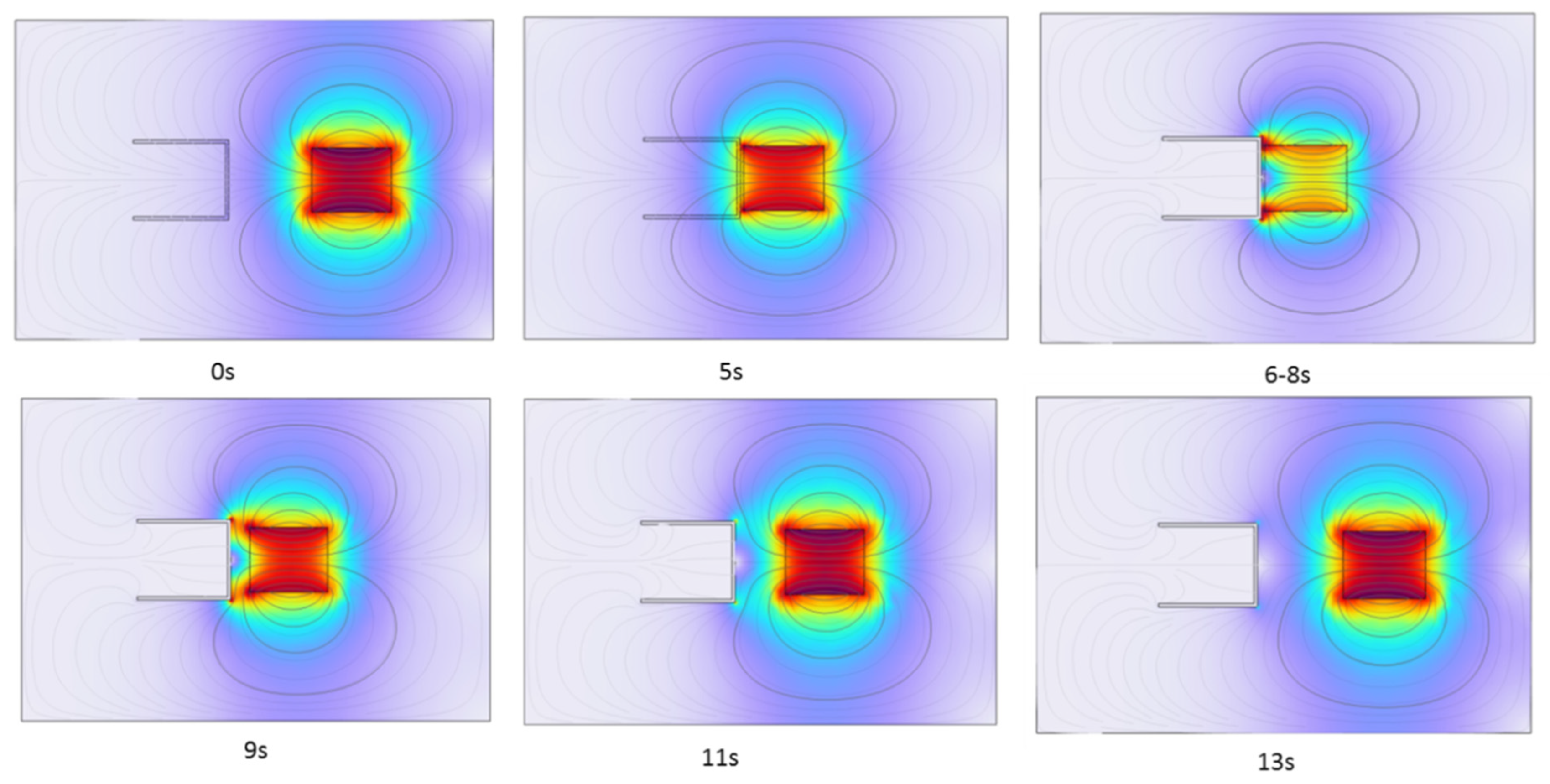
Figure 14. Electromagnetic field distribution at various time points in the model without moving magnets.

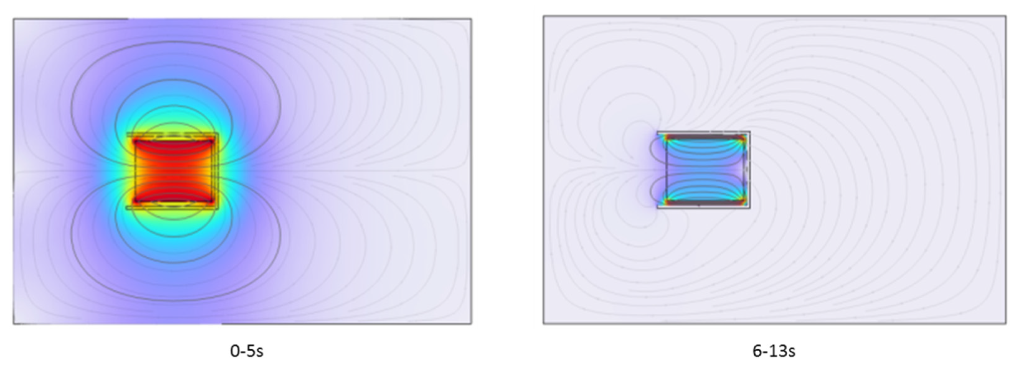
Figure 15. Magnetic Flux Density Modulus at Point 1 in the Complete Model.

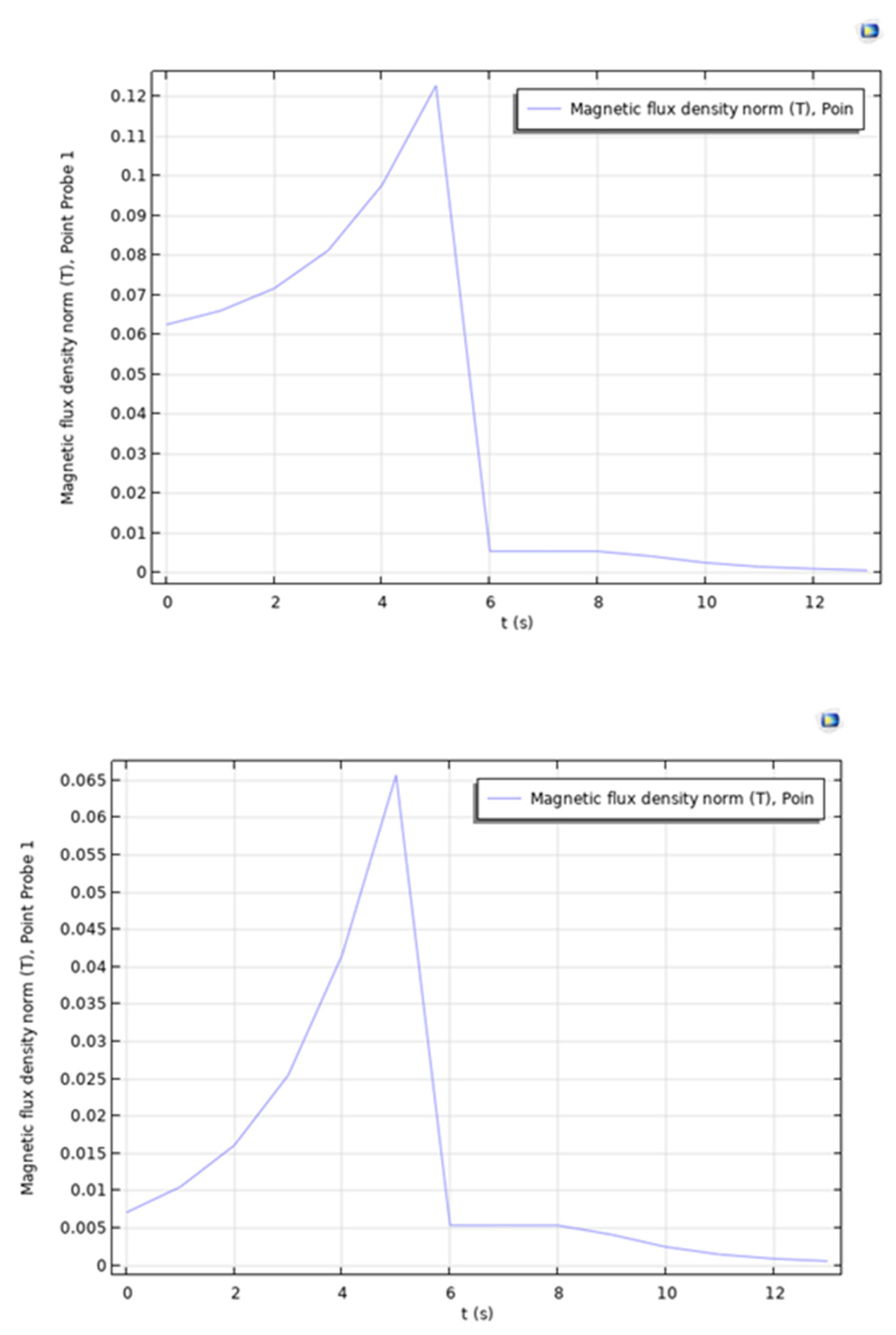
Figure 16. Magnetic Flux Density Modulus at Point 1 in the Model Without a Fixed Magnet.

Figure 17. Comparison of magnetic flux density modulus curves at Point 1 for the three combinations.

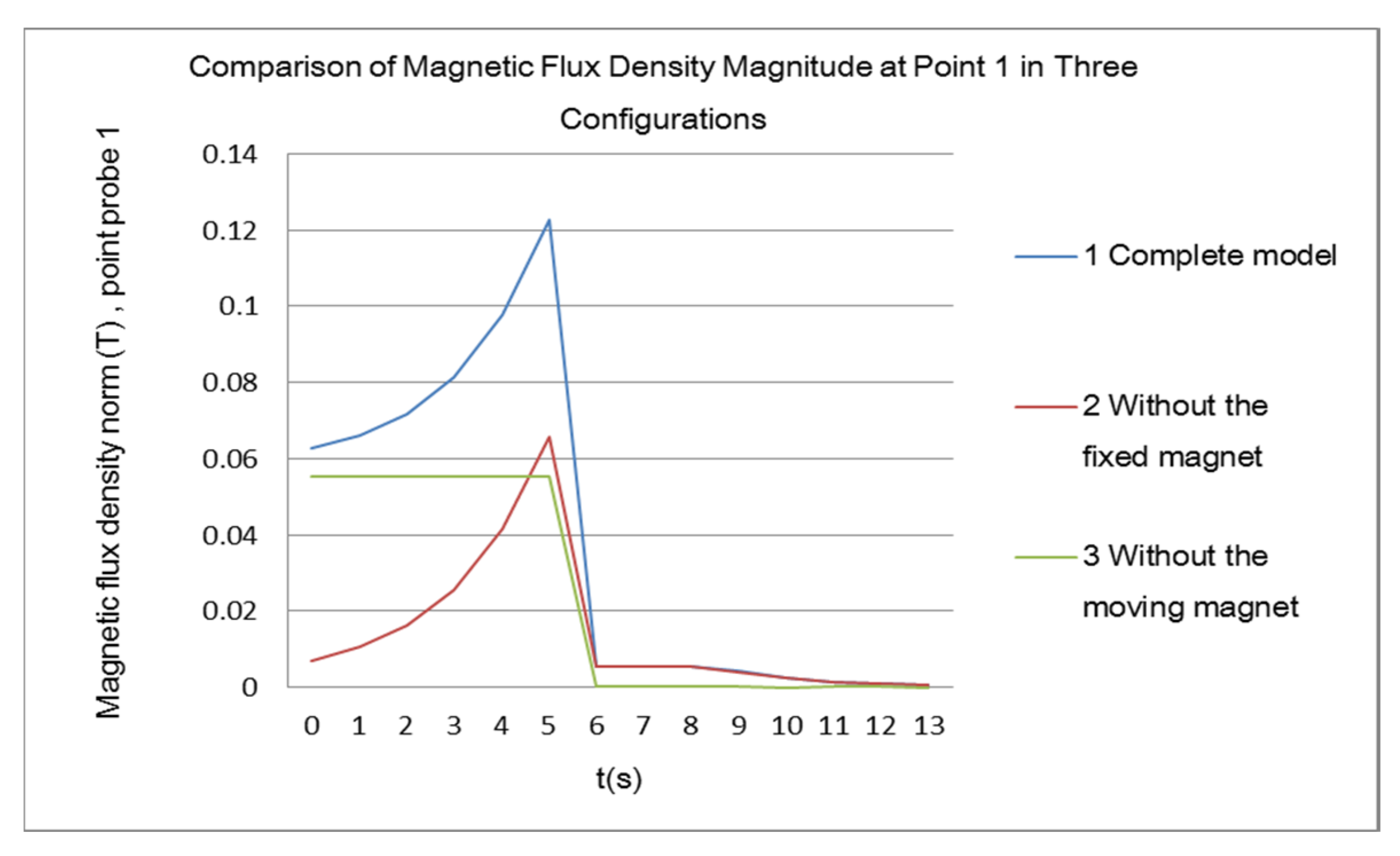
Figure 18. Electromagnetic force on the moving magnet in the complete model.

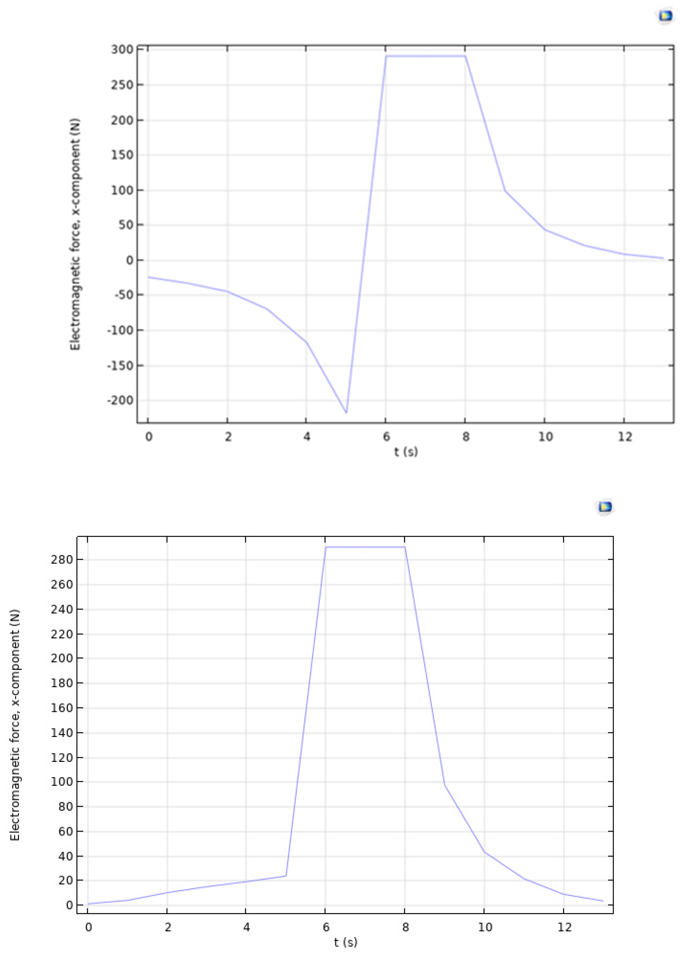
Figure 19. Electromagnetic force on the moving magnet in the model without the fixed magnet.

Figure 20. Electromagnetic force on the moving magnet for the two combinations.

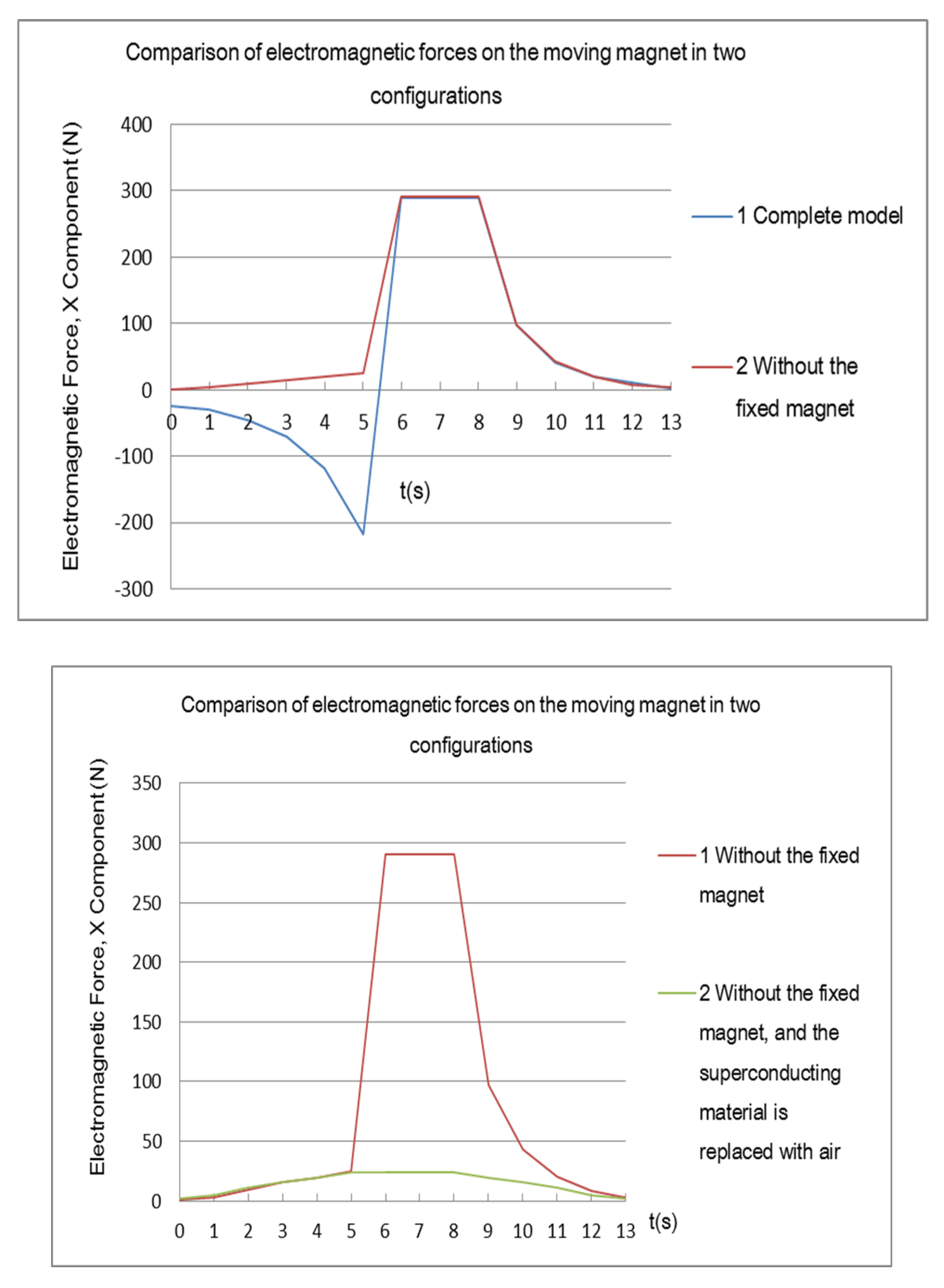
Figure 21. Electromagnetic force on the moving magnet for the other two combinations.

Figure 26. Summary of the simulation data.

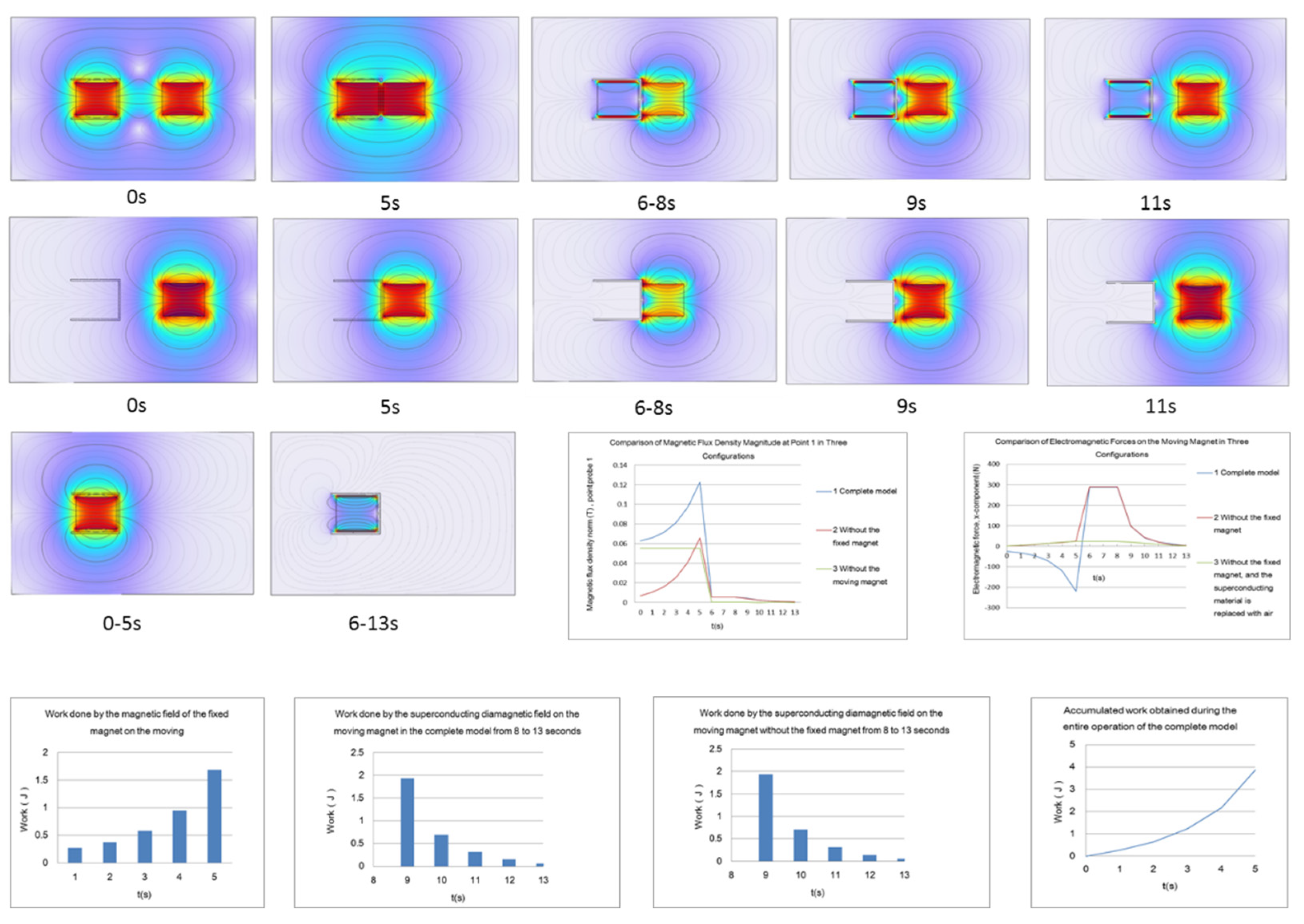
Figure 27. Experimental Setup for Model Verification.

Disclaimer/Publisher’s Note: The statements, opinions and data contained in all publications are solely those of the individual author(s) and contributor(s) and not of MDPI and/or the editor(s). MDPI and/or the editor(s) disclaim responsibility for any injury to people or property resulting from any ideas, methods, instructions or products referred to in the content.

© 2024 by the authors. Licensee MDPI, Basel, Switzerland. This article is an open access article distributed under the terms and conditions of the Creative Commons Attribution (CC BY) license (http://creativecommons.org/licenses/by/4.0/).

Copyright: This open access article is published under a Creative Commons CC BY 4.0 license, which permit the free download, distribution, and reuse, provided that the author and preprint are cited in any reuse.