
Submitted:
09 January 2025
Posted:
10 January 2025
Read the latest preprint version here
Abstract
The rapid evolution of intelligent vehicle technology has significantly advanced autonomous decision-making and driving safety. However, the challenge of predicting long-term trajectories in complex urban traffic persists, as traditional methodologies usually handle spatiotemporal attention mechanisms in isolation and are typically limited to short-term trajectory predictions. This paper proposes a Habit-based Temporal-Spatial Attention Long Short-Term Memory (HTSA-LSTM) network, a novel framework that integrates a dual spatiotemporal attention mechanism to capture dynamic dependencies across time and space, coupled with a driving style analysis module. The driving style analysis module employs Sparse Inverse Covariance Clustering and Spectral Clustering (SICC-SC) to extract driving primitives and cluster trajectory data, thereby revealing diverse driving behavior patterns without relying on predefined labels. By segmenting real-world driving data into fundamental behavioral units that reflect individual driving preferences, this approach enhances the model's adaptability. These behavioral units, in conjunction with the spatiotemporal attention outputs, serve as inputs to the model, ultimately improving prediction accuracy and robustness in multi-vehicle scenarios. The model was evaluated by using the NGSIM dataset and real driving data from Wuhan, China. In comparison to benchmark models, HTSA-LSTM achieved a 20.72% reduction in root mean square error (RMSE) and a 24.98% reduction in negative log likelihood (NLL) for 5-second predictions of long-term trajectories. Furthermore, HTSA-LSTM achieved R² values exceeding 97.9% for 5-second predictions on highways and expressways and over 92.7% for 3-second predictions on urban roads, highlighting its excellent performance in long-term trajectory prediction and adaptability across diverse driving conditions.
Keywords:
Trajectory prediction
; Long Short-Term Memory (LSTM)
; spatiotemporal attention
; Driving Style Analysis
; autonomous driving
; real-world driving data
; model analysis
1. Introduction
Intelligent vehicles, equipped with advanced sensing systems, are transforming the way we perceive and navigate driving environments. These vehicles can gather extensive amounts of contextual information, surpassing the capabilities of human drivers. This advanced perceptual capability serves as a critical foundation for comprehending the driving environment and making accurate decisions in autonomous vehicle operations. Based on these sensor inputs, autonomous vehicles must infer the intentions of surrounding vehicles and accurately predict their future trajectories [1,2]. Such highly accurate trajectory predictions are crucial not only for anticipating upcoming driving conditions but also for informing the subsequent tactical decisions of autonomous vehicles [3].
In the context of complex urban road networks, decision-making in intelligent vehicles is ultimately reflected in their trajectory and driving behavior. Predicting a vehicle’s future trajectory is therefore a pivotal factor in ensuring safety in dynamic traffic conditions [4]. Furthermore, trajectory prediction is indispensable for modeling traffic states, facilitating decision-making, planning, and anticipating hazards. Accurately forecasting the movements of nearby vehicles is essential for the effective operation of intelligent vehicles. Yet, achieving consistent precision in trajectory predictions, particularly in challenging environments, remains a notable challenge [5]. Simultaneously, the diversity in driving behaviors and the inherent complexity of urban traffic also pose considerable challenges to achieving reliable and accurate predictions [6].
Traditional trajectory prediction models often overemphasize historical trajectory data, neglecting the fact that their influence may diminish over time. It is essential to evaluate the relevance of historical features across varying temporal horizons [7]. Moreover, many models address temporal and spatial attention independently, thereby overlooking their interdependencies. Beyond spatial feasibility and target positions, a driver's style plays a significant role in influencing trajectory modifications. To enhance accuracy and stability, these challenges must be systematically addressed [8,9].
Recent studies [10] categorize vehicle trajectory prediction approaches into four primary methodologies: physical models, machine learning, reinforcement learning and deep learning. Among these, traditional methods, such as dynamic models, kinematic models [11], Kalman filtering [12], and Monte Carlo methods [13], utilize features like vehicle speed, acceleration, and turning rate. Although these approaches are computationally efficient, they often struggle to maintain accuracy in complex traffic scenarios. Machine learning approaches have introduced new paradigms for trajectory prediction. For example, Bahram et al. [14] integrated model-driven interaction perception with supervised learning, while Zhu et al. [15] employed SVM and GMM to analyze multi-participant interactions. However, these models often require deterministic maneuver characteristics, limiting them to simpler, short-term scenarios. Reinforcement learning (RL) has emerged as a promising framework for managing the complexity and high-dimensionality of driving environments. Approaches such as HRL [16] and GAIL [17] have demonstrated efficacy in autonomous driving policy learning. However, RL’s computational intensity and lengthy training times hinder its feasibility for real-time applications.
Deep learning has gained significant prominence, marked by advancements in sequence models, graph neural networks (GNNs), and generative models. Sequence networks extract feature sequences from trajectory data, with models such as MFP [18] and mmTransformer [19] integrating environmental context for enhanced predictions. GNNs, such as TrGNN [20] and hierarchical GNN models [21], capture interdependencies among traffic participants. Generative Adversarial Networks (GANs) have been applied to analyze multimodal trajectory distributions, as seen in GAN-VEEP [22] and ME-GAN [23]. Generally, deep learning approaches outperform traditional methods in terms of both accuracy and scalability. GCN-based Prediction [24] uses spatial and temporal graphs in connected environments, highlighting its advantage in cooperative driving scenarios. Attention-based GCN [25] introduces a novel use of vehicle-to-traffic rule interactions, offering enhanced prediction in complex environments such as intersections. Feature-Boosting Network [26] emphasizes feature enhancement techniques, achieving remarkable gains in trajectory prediction accuracy through its novel high-dimensional space analysis. L. Lin et al. introduced the STA-LSTM model incorporating an attention mechanism in 2022 [27].
While deep learning models generally deliver robust prediction accuracy, they often face challenges in identifying key historical moments and influential neighboring vehicles. The STA-LSTM model’s spatial-temporal attention mechanism highlights crucial trajectory points and evaluates the influence of surrounding vehicles, enhancing interpretability. However, the 1-second prediction horizon of the model constrains its practical applicability and raises potential safety concerns. Moreover, while the model enhances interpretability, this improvement does not result in a significant increase in accuracy when compared to more advanced models such as CS-LSTM. The grid-based spatial modeling approach, while simplifying computational processes, is insufficient for capturing the intricate interactions present in dynamic environments. To address these limitations, future work should consider incorporate advanced data structures, such as graph neural networks (GNNs). Moreover, the STA-LSTM model's predominant emphasis on highway scenarios restricts its applicability to diverse urban environments, necessitating further validation to ensure the model's accuracy in trajectory prediction on urban road networks.
Accurate trajectory prediction must take into account both the temporal continuity of vehicle motion and the spatial influence of surrounding vehicles. Current research often neglects driver behavior variability, hindering personalized intelligent systems. This study establishes a road network using a fixed reference frame centered on the target vehicle, discretizing the surrounding road space into a 3×13 grid (Figure 1). By integrating driver behavior variability, the model achieves long-term trajectory prediction while accounting for different driving styles in multi-vehicle scenarios.
In this study, we developed an enhanced trajectory prediction model based on Long Short-Term Memory (LSTM) networks, named HTSA-LSTM. This model integrates spatiotemporal attention mechanisms and accounts for variations in driving behavior, specifically designed for long-term trajectory prediction in multi-vehicle interaction scenarios, predicting the potential positions a target vehicle may reach within the forecast horizon. The main contributions of this work are as follows:
- Dynamic Spatiotemporal Attention Mechanism: This mechanism captures essential spatiotemporal dependencies between moving vehicles by integrating dynamic temporal and spatial attention. The model selectively identifies critical moments within historical traffic data and dynamically adjusts weight distributions according to real-time traffic conditions, enhancing its adaptability. This capability significantly improves prediction accuracy, especially in rapidly changing traffic environments, demonstrating the model’s effectiveness in handling complex, evolving scenarios.
- Driver Behavior Analysis Module: This module segments time-series driving data into behavioral units, enhancing prediction accuracy by incorporating historical trajectories. Driving primitives are extracted through a Sparse Inverse Covariance Clustering (SICC-SC) method, clustering trajectory data to reveal distinct behaviors without predefined labels, achieving robust adaptability. Temporal consistency is maintained via a dynamic programming-based Expectation-Maximization (EM) framework, while a Toeplitz graphical Lasso with ADMM refines model sparsity, enabling precise and interpretable risk analysis and demonstrating effectiveness in complex, multi-vehicle scenarios.
- Real-World Model Validation: Extensive data collection experiments were conducted across diverse road conditions in Wuhan, China, to assess the model’s generalization and effectiveness. Data from 20 drivers were collected over 12 kilometers of urban roads, 34 kilometers of expressways, and 45 kilometers of highways. After preprocessing, this dataset validated the HTSA-LSTM model's performance under real-world driving conditions, demonstrating its robustness and applicability in varied traffic environments.
In summary, this study introduces the HTSA-LSTM model, which integrates dynamic spatiotemporal attention mechanisms and variations in driving behavior to improve the prediction of future vehicle trajectories. The following sections will discuss the model’s architecture, the principles of the spatiotemporal attention mechanism, the training and evaluation using the NGSIM dataset, and the validation of its effectiveness with real-world driving data.
2. Model Development
In urban road network systems, straight road segments constitute the primary road form. Therefore, this chapter focuses on the driving states of traffic participants on straight road segments. A fixed reference frame is employed in this study, with the origin fixed at time t at the geometric center of the target vehicle's vertical projection onto the road surface [28], as shown in Figure. 1. In this reference frame, the y-axis aligns with the direction of the target vehicle's motion on the road, while the xxx-axis is perpendicular to the vehicle's motion direction.
The historical trajectory of a traffic participant is defined as a numerical vector, where the values alternate between and and are separated by fixed time steps corresponding to the device's sampling frequency. A trajectory consisting of n points is represented as a sequence of values ,,,…,, all of which are elements of the set T, defined as follows:
The trajectory point indices are mapped to timestamps through the function , which follows the conditions specified in Equation 2, where is the fixed time step:
In this chapter, the trajectory prediction problem is defined as the following sequence generation task: Given an observed trajectory of m<n points as the sequence , , the goal is to predict each as accurately as possible by minimizing some error metric between the actual and predicted trajectories.
In the HTSA-LSTM trajectory prediction model proposed in this chapter—based on LSTM, integrating spatiotemporal attention mechanisms, and accounting for differences in driver behavior—a fixed reference frame is used, as illustrated in Figure 2. The model's output is defined as:
whererepresents the instantaneous coordinates of the target vehicle and the neighboring vehicles in adjacent lanes within a distance meters at time . The specific value of must comply with local traffic safety regulations, matching the safe distance required at the current driving speed.
The model's output is a probability distribution of the possible trajectory:
where represents the coordinates that the target vehicle may reach within the prediction time steps .
2.1. Traditional Models
When utilizing traditional neural networks for time series predictions, a significant limitation arises due to the network's inherent disregard for whether information from a preceding time frame might influence tasks in subsequent moments. This oversight renders traditional neural networks unsuitable for time series problems. In the context of vehicle trajectory prediction, it is indisputable that driving data from previous time intervals has a substantial impact on subsequent prediction tasks. To address this issue of "long-term dependency," Long Short-Term Memory (LSTM) recurrent neural networks were introduced. These LSTM units are capable of analyzing temporal dependencies within the input data to the network. By incorporating gating mechanisms, LSTM units enhance the memory capabilities of standard recurrent units. Specifically, an LSTM consists of a forget gate, an input gate, an output gate, and a memory cell (as illustrated in Figure. 2). Several variants of the standard LSTM have emerged, such as LSTMs without forget gates and those with peephole connections. However, in the HTSA-LSTM model, all LSTMs utilized are standard LSTM units. Figure. 2 illustrates the traditional LSTM architecture.
Forget Gate: Upon receiving input into the LSTM unit, the first task of the LSTM is to determine which information from the cell state should be discarded, or "forgotten." This decision is governed by the "forget gate layer" of the network. The forget gate accepts two input variables: the output value from the previous time step and the current input value . After processing through the forget gate, the resulting information , which represents the magnitude of information to be discarded, is obtained. Each value in the cell state is scaled within the range [0, 1], where 1 indicates "fully retain this state," and 0 indicates "completely disregard this state." The forget gate update is as follows:
where is the weight matrix, is the bias term, is the output value from the previous network unit, is the current network input, and is the sigmoid function.
Input Gate: After information has been filtered through the forget gate, it is necessary to determine which information should be preserved in the LSTM cell state. This functionality is primarily achieved through the "input gate" layer and the tanh layer. The "input gate" layer primarily decides which information should be updated, while the tanh layer creates a new candidate vector that can be integrated into the cell state update. The input gate update is as follows:
where and are the weight matrices, and are the bias terms, and tanh refers to the hyperbolic tangent function.
LSTM Cell State Update: The process of updating the cell state involves transitioning the old state to the new state . Following the selection of information by the forget gate and the input gate, the cell state is multiplied by the value determined by the forget gate. This result signifies that the forget gate has opted to discard certain information. Subsequently, the value from the input gate is multiplied by the candidate vector and added to the output from the forget gate, thereby incorporating some new information into the cell state. The cell state update is expressed as:
where represents the weight from the forget gate, denotes the output of the forget gate, is the value from the input gate, and represents the new candidate value. This value is scaled according to the network's updates for each cell state.
Output Gate: The determination of the output value is contingent upon the updated cell state. This value is derived by passing the current input and the hidden state from the previous time step through a fully connected layer, followed by the application of a function, which yields the output value within the range [0, 1]. A value of 0 indicates no output, while a value of 1 indicates full output. The cell state is then processed through a function to produce a result within the range of [-1, 1], which is multiplied by the output gate value to obtain the final hidden state:
where is the weight matrix, and is the bias term.
2.2. Attention Mechanism
Traditional models treat temporal and spatial attention independently. In contrast, the HTSA-LSTM model integrates these mechanisms, allowing them to interact and influence one another, resulting in more accurate predictions. The following sections will detail the working principles of the dynamic spatiotemporal attention mechanism and its advantages in real-world applications.
2.2.1. Temporal Attention Mechanism
In the HTSA-LSTM model, at a given time step, the T-step historical trajectories of the target vehicle and its neighboring vehicles, denoted as , are used as the input to the model. Considering the hidden states of the LSTM units in HTSA-LSTM, , with d representing the length of the hidden state. After generating these hidden states, the temporal attention weights associated with v, denoted as , are computed as follows:
where represents the learnable weights.
Next, by combining the hidden states with the temporal attention weights , the tensor cell value associated with vvv is derived as follows:
Overall, all tensor cell values are utilized to compute the spatial-level attention weights and to predict the trajectory of the target vehicle.
2.2.2. Spatial Attention Mechanism
In the HTSA-LSTM model, the tensor cell values at time t are represented as follows:
where N denotes the total number of tensor cells (N=3×13=39). The tensor cell is defined as follows:
The spatial attention weights associated with all vehicles at time t are computed as follows:
where represents the learnable weights.
Here, represents the spatial attention weights corresponding to each cell at time t. Finally, the historical information of the target vehicle and its neighboring vehicles is aggregated as follows:
Subsequently, the spatiotemporal interaction information is coupled with the driving style information.
In the HTSA-LSTM model, there is a strong interdependence between the temporal attention mechanism and the spatial attention mechanism. This relationship is manifested primarily in the following two aspects:
Temporal Attention Mechanism: The model applies weighted processing to the T-step historical trajectory data of the target vehicle and its neighboring vehicles, generating a weighted hidden state for each time step. This process focuses on assigning appropriate weights based on the significance of historical data, thereby highlighting the most critical moments for future trajectory prediction. These weighted hidden states are subsequently integrated into the spatial attention mechanism, forming the tensor cell values . Specifically, if vehicle is within network cell , is included as part of ; otherwise, is set to zero. This demonstrates that the output of the temporal attention directly influences the input structure of the spatial attention mechanism.
Spatial Attention Mechanism: This mechanism leverages the tensor cell values of all vehicles, including the output from the temporal attention mechanism, to calculate the spatial attention weights . This step emphasizes identifying the regions within the various spatial cells (or network cells) that have the most significant impact on predicting the target vehicle's trajectory. The model then performs a weighted sum of all using the weights , generating the final representation that integrates both temporal and spatial information, as described in Equation 17.
2.3. Driving Style Analysis Module
To better utilize sensor data and capture driving styles, temporal state continuity is introduced to segment and cluster vehicle sensor data. A sparse inverse covariance clustering method based on temporal sequence state continuity (SICC-SC) was developed. For semantic analysis of driving primitives, a network analysis method is applied. Using the network structure of each driving primitive obtained from SICC-SC, the driving primitives are semantically interpreted and defined without manually predefined labels. The SICC-SC method is used to segment the driver's trajectory data, resulting in five clusters.

Table 1.
Centrality Score of Network Nodes.
| Driving Primitives | Explanation | |
|---|---|---|
| #0 | Stable High Speed | |
| #1 | Stopping | |
| #2 | Accelerating | |
| #3 | Low Speed | |
| #4 | Turning |
As shown in Figure 3, after obtaining the multidimensional vehicle sensor data, a sliding window with a size of is used to extract local time-series data. First, the relative distance series of neighboring data points within the window is calculated, including the mean and standard deviation . Based on the characteristics of the normal distribution, each value in is assigned a similarity metric, representing the temporal continuity of the time series. Subsequently, the Expectation-Maximization (EM) algorithm is used to solve the sparse inverse covariance matrix Θ.
A dynamic programming (DP)-based clustering assignment method is introduced to address the issue of state continuity in time series data. In the E-step of the EM algorithm, the combinatorial optimization problem is solved by maximizing the expected likelihood. The objective function minimizes the sum of the negative log-likelihood and a penalty term :
where governs the state continuity between adjacent time points. A larger increases the likelihood that neighboring points are assigned to the same cluster. The method computes the optimal path with minimal cost using dynamic programming, ensuring the appropriate clustering of time series data.
Once the cluster assignment result P is obtained, the cluster parameters are then updated. We propose an optimization method based on the Toeplitz graphical Lasso, solved using the Alternating Direction Method of Multipliers (ADMM). The objective function maximizes the log-determinant of the Toeplitz covariance matrix while adding a Lasso sparsity regularization term:
where Θ is the covariance matrix, S is the empirical covariance matrix, and λ controls the sparsity. The ADMM iteratively updates Θ, Z, and the Lagrange multiplier U, solving the optimization problem in a recursive manner. The update steps involve optimizing the log-determinant for Θ, applying Lasso sparsity constraints to Z, and updating the Lagrange multiplier U to enforce the constraintEach cluster is represented by an inverse covariance
matrix , defined
as the driving basis, also known as the precision matrix. The dimensionality of
this matrix is , which represents the conditional independence relationships between the six sensors. Due to the block Toeplitz structure of the inverse covariance matrix, assuming a window size of 2, the time-invariant assumption can be made, allowing better representation of the temporal relationships between the sensors. On one hand, the diagonal blocks represent the temporal correlations of the same sensor across different time points, while the off-diagonal blocks represent the conditional correlations between different sensors at the same time. The element in the matrix indicates that the sensor variables and are conditionally independent. Conditional dependencies are denoted as . The dependency relationship is represented by the formula:
In this paper, a threshold of is set to convert the matrix into a graph structure. Edges with weights lower than the threshold are removed, while edges with weights higher than the threshold are retained, and their weights are represented by the relative bias coefficient
. Afterward, the distribution of the standardized driving primitives is used to analyze the statistical properties and risks of different drivers. We standardized the characteristics of the driver and input them into the HTSA-LSTM.
2.4. Coupled Spatiotemporal Attention Model Considering Driving Styles
The architecture of the HTSA-LSTM model is illustrated in Figure 4. To predict vehicle trajectories within a road network, the model leverages temporal and spatial attention mechanisms to capture dependencies in both time and space. Additionally, it integrates a driving style analysis module to account for the influence of varying driving behaviors on vehicle movement. The road network surrounding the target vehicle is discretized into a 3×13 grid, as shown in Figure 1. The grid's rows represent the left, current, and right lanes relative to the target vehicle, while the columns correspond to discrete grid cells of width L [m], determined by the vehicle's length and the driving environment. In alignment with related studies [28], L is set to 4.6 m (15 ft) during training with the NGSIM dataset. All vehicles within the 3×13 grid, excluding the target vehicle, are considered neighboring vehicles, each occupying a unique grid cell.
The input to the HTSA-LSTM model consists of the historical trajectories over T steps and the driving style information of all vehicles within the grid. The model outputs the predicted trajectory of the target vehicle for the next H steps. The temporal attention mechanism analyzes the influence of historical trajectories of both the target and neighboring vehicles, while the spatial attention mechanism captures the impact of the surrounding environment on the prediction. Integration module driving styles analyze is used to obtain driving habits.
In summary, the HTSA-LSTM model effectively integrates temporal and spatial attention mechanisms, combining time-series analysis with spatial feature recognition. The temporal attention identifies critical relationships between past trajectories and the current state, while the spatial attention emphasizes key environmental features. By employing a dynamic spatiotemporal attention mechanism, the model captures evolving spatiotemporal dependencies and incorporates driving style variations, enhancing its understanding of the interaction between these factors for more accurate trajectory predictions.
3. Experiments and Evaluation
This chapter explores and validates the application of the temporal-spatial attention mechanism-based Long Short-Term Memory (HTSA-LSTM) model for vehicle trajectory prediction. Using the NGSIM US101 trajectory dataset for analysis and model training, we demonstrate the superiority of the HTSA-LSTM in handling complex traffic scenarios. Comparisons with benchmark models further validate its advantages in prediction accuracy and generalization capability. Additionally, the model's effectiveness in real-world driving conditions was confirmed using actual vehicle driving data.
During the dataset segmentation and model training phase, the data was split into training, validation, and test sets with a 7:1:2 ratio. The model inputs consisted of time series segments, enabling precise future trajectory predictions. The configuration and optimization of model parameters, along with the experimental environment setup, laid a strong foundation for the research. This chapter also provides a detailed listing of the model’s hyperparameters, serving as a reference for future experiments and comparisons. All experiments were conducted using Python 3.8, CUDA 11.6.2, a 12-core Intel Xeon Platinum 8255C @ 2.50GHz CPU, an Nvidia RTX 3080 (10GB) GPU, and 40GB of RAM.
3.1. Formatting of Mathematical Components
To assess the effectiveness of the HTSA-LSTM model in real-world applications, this section separately trains and tests the model using real-world driving data from urban city roads (CRS), urban expressways (UES), and highways (HS). The following evaluation metrics are employed to evaluate the model's performance on the test set:
1. Root Mean Square Error (RMSE):
RMSE is a common metric for evaluating the accuracy of a model's predictions. However, it has certain limitations when assessing the accuracy of multimodal predictions, as RMSE tends to favor models that average the prediction results. In some specific scenarios, the mean value may not accurately reflect the quality of the prediction.
2. Negative Log-Likelihood Loss (NLL):
To address this limitation, another evaluation metric is introduced: the negative log-likelihood loss (NLL) of the model's predicted trajectory relative to the corresponding true trajectory [29]. Although the NLL value cannot be directly interpreted as a specific physical quantity, it provides an intuitive comparison between unimodal and multimodal prediction distributions.
The trajectory information input into the HTSA-LSTM model is denoted as , comprising a series of trajectory points continuously distributed over time. For each , there is a corresponding predicted point . The probability distribution of the predicted trajectory points at each position, represented as reflects the prediction accuracy at point , abbreviated as. The goal is for the HTSA-LSTM model's prediction accuracy to be as close to 1 as possible for each trajectory point. The objective of the negative log-likelihood loss (NLL) is to minimize the negative log of , or , which encourages the prediction accuracy to approach 1, thereby minimizing the loss and reducing the discrepancy between the predicted and true values. The NLL of the input data is the average NLL across all samples, where NNN represents the number of trajectory points in the input data.
3. Mean Absolute Error (MAE):
MAE ranges from [0, +∞), where smaller MAE values indicate that the predictions are closer to the true values. An MAE of 0 suggests that the model is perfect; conversely, larger prediction errors result in a higher MAE.
4. R-Squared (R²) Coefficient of Determination:
R² ranges from [0, 1] and is used to characterize the fit of the model's predictions to the actual data.
3.2. Dataset Segmentation and Model Training
Figure 5 illustrates the data segmentation process. This chapter utilizes the preprocessed NGSIM US101 trajectory dataset, which is discretized and mapped according to the road network structure shown in Figure 1. The NGSIM dataset records vehicle movement data on highways, primarily capturing forward driving and lane-changing behaviors. The US101 dataset includes three 15-minute trajectory segments (7:50 am–8:05 am, 8:05 am–8:20 am, 8:20 am–8:35 am), which are divided into training, validation, and test sets in a 7:1:2 ratio. During model training, a specific vehicle is selected as the objective vehicle (OV), while the surrounding vehicles within a 3×13 road grid are considered neighboring vehicles (NV).
In the HTSA-LSTM model, the historical trajectory data of the OV and NV over T seconds is used to predict the OV's trajectory over the next H seconds. Therefore, each feature sequence segment must be at least T+H seconds long (as illustrated in Figure 5). In this study, the vehicle trajectory data is segmented into time series fragments of T+H seconds, where T seconds represents the OV's historical driving data, and H seconds represents the model's future trajectory prediction range. Both are sampled at a frequency of 10 Hz. Data segmentation is performed using a sliding time window of length T+H, allowing the predicted results to be merged into a continuous sequence, thus enabling predictions over longer time horizons. Before inputting the data into the HTSA-LSTM model, each vehicle's trajectory is down sampled by a factor of 2 to reduce model complexity.
Model Parameter Settings: Based on existing research results in trajectory prediction and considering subsequent comparative experiments, the length of the output window H in the HTSA-LSTM model is incrementally increased from 1, selecting the optimal future prediction step length according to the evaluation metrics. Hyperparameters in the model are optimized using grid search, with the final parameter settings provided in Table 2. For the parameter setting of SICC-SC, we refer to the previous work [30]
3.3. Training Setup and Evaluation Metrics
To comprehensively account for the influence of driving style on vehicle trajectory, a driving style analysis module has been embedded within the HTSA-LSTM model. This module performs semantic parsing of the input data, identifying and segmenting fundamental driving behavior units, thereby enabling an unsupervised analysis of the driver's driving style. By incorporating the driving style analysis module, the model not only captures temporal and spatial dependencies through the spatiotemporal attention mechanism but also integrates the impact of driving style into the analysis.
3.4. Results and Comparison
In this chapter, the NGSIM US101 dataset is utilized to predict future vehicle trajectories using the HTSA-LSTM model alongside several baseline models. The performance of these models is evaluated using RMSE and NLL metrics. The baseline models assessed include:
- Constant Velocity (CV) [31]: An earlier trajectory prediction method based on physical principles, primarily using the vehicle's dynamic model and Kalman filter equations. Although the dataset lacks factors like road surface friction, making complex physics-based comparisons impractical, a simple physics-based model is constructed to predict the vehicle's trajectory under constant velocity.
- Simple-LSTM (S-LSTM) [32]: This model uses LSTM units within a recurrent neural network to analyze continuous time-series data for temporal vehicle trajectory predictions.
- Maneuver-LSTM (M-LSTM) [33]: Based on an encoder-decoder framework, this model uses historical trajectory data and lane structure, assigning confidence values to six maneuver categories to predict future motion through a multimodal distribution.
- Attention-LSTM (A-LSTM) [34]: This model uses an LSTM encoder with shared weights to generate vector encodings of each vehicle’s motion. An attention module models interactions based on the importance of adjacent vehicles, and the decoder uses these interaction vectors to predict trajectory distribution.
- Convolutional Social Pooling LSTM (CS-LSTM) [27]: This model, based on an LSTM encoder-decoder framework, employs a social convolutional network to accurately capture spatial interactions among agents, producing multimodal trajectory predictions.
- Spatial-Temporal Attention-LSTM(STA-LSTM) [1]: This model employs an LSTM encoder-decoder framework with integrated spatial and temporal attention mechanisms. It assigns weights to surrounding vehicles and historical time steps, capturing critical interactions for trajectory prediction. STA-LSTM enhances the accuracy of multimodal trajectory predictions by effectively modeling dynamic relationships over time and space.
Comparative models (4) and (5) serve as ablation experiments for HTSA-LSTM, with A-LSTM using only a unified attention mechanism (AM) and CS-LSTM employing only the spatial attention mechanism (social convolutional network). HTSA-LSTM integrates both, with AM as the temporal attention mechanism and the social convolutional network as the spatial attention mechanism. Models (2) and (3) also contribute to a broader ablation study, where removing the spatiotemporal attention from HTSA-LSTM results in S-LSTM, and replacing it with a Maneuver module results in M-LSTM, retaining the overall framework while altering specific components.
Table 3 presents the RMSE and NLL values for predictions made by HTSA-LSTM and baseline models on the NGSIM US101 dataset. As shown, the evaluation metrics increase as the prediction horizon extends, indicating a decline in prediction accuracy for all models. Compared to other baseline models, the CV and S-LSTM models produce higher RMSE and NLL values, which can be attributed to the fact that other models consider the influence of interaction information from neighboring vehicles during trajectory prediction. This directly indicates the significance of vehicle interaction information in trajectory prediction. The results for prediction horizons of 1 to 6 seconds demonstrate that HTSA-LSTM yields significantly lower RMSE and NLL values than other baseline models, indicating higher accuracy in predicting future vehicle trajectories.
The analysis of the RMSE and NLL values for STA-LSTM and HTSA-LSTM models reveals significant differences in their performance across prediction horizons. As with the overall trend observed in Table 3, both models show increased RMSE and NLL values as the prediction horizon extends, indicating a decline in accuracy. However, HTSA-LSTM consistently outperforms STA-LSTM across all time frames, demonstrating its superior ability to incorporate vehicle interaction information into trajectory predictions. Specifically, HTSA-LSTM achieves markedly lower RMSE and NLL values compared to STA-LSTM, particularly in the shorter prediction horizons, highlighting its effectiveness in accurately forecasting future vehicle trajectories. This emphasizes the importance of utilizing interaction data from neighboring vehicles for improved prediction accuracy.
3.5. Analysis of Temporal and Spatial Attention Allocation
Following the overall analysis of the HTSA-LSTM model's trajectory prediction performance, this section delves into the allocation of the temporal attention mechanism across time steps and the spatial attention mechanism within the road network structure.
3.5.1. Temporal Attention Allocation
This analysis uses three 15-minute subsets from the NGSIM US101 dataset to examine the allocation of temporal attention, calculating the attention weights for 15 historical time steps (from to ). Figure 6 illustrates the average temporal attention weights from to . It is evident that the weights before are nearly zero, indicating minimal influence on the prediction results, and thus, the model opts to ignore them. The temporal attention weight at the current time step is the highest, suggesting that the future trajectory of the target vehicle is primarily influenced by the most recent state of the target and neighboring vehicles. This result also explains why the CS-LSTM model, which incorporates spatial but not temporal attention, underperforms compared to HTSA-LSTM.
3.5.2. Spatial Attention Allocation
The study section of US101 in the NGSIM dataset comprises five lanes, with each section including an on-ramp. Figure 7 is a lane distribution map at the Ventura Boulevard on-ramp, captured from Google Maps. This chapter selects four lanes from the southbound section of Ventura Boulevard on US101: the innermost lane, the middle lane, the outermost lane, and the on-ramp section (corresponding to the lanes indicated by the blue, green, yellow, and red arrows, respectively, in the figure) to analyze the spatial attention allocation of the target vehicle in different lanes.
In analyzing the spatial attention mechanism's weight distribution, each road network grid cell is labeled based on the lane name and its relative position to the target vehicle’s grid cell. To simplify, the following abbreviations are used: Current Lane (C), Right Lane (R), and Left Lane (L). The longitudinal representation of the lane grid is illustrated in Figure 8, with values ranging from -6 to 6. For example, (C, 0) represents the target vehicle’s position, (C, 6) indicates the sixth grid cell ahead in the current lane, (R, 2) denotes the second grid cell ahead in the right lane, and (L, -3) refers to the third grid cell behind in the left lane. Regarding spatial attention weights, the grid cell occupied by the target vehicle holds the highest attention weight at 71.56%. This, combined with the temporal attention weight distribution, suggests that the target vehicle’s future trajectory is predominantly influenced by its own driving state. The study focuses on passenger vehicles, which are highly maneuverable and can quickly adjust their trajectories in response to surrounding vehicles.
To better describe the distribution of attention weights among neighboring vehicles in the road network structure, the remaining 28.44% of attention weights, excluding the 71.56% allocated to the target vehicle, are normalized and distributed across the 3×13 road grid. The results are shown in Figure 8. It can be observed that the grid cells behind the target vehicle receive very little attention, indicating that rear vehicles have a minimal impact on the target vehicle, and drivers pay less attention to the dynamics of vehicles behind them.
Figure 8 further shows that the target vehicle's spatial attention is primarily focused on vehicles ahead in the current lane. However, the on-ramp section is an exception, where the target vehicle pays more attention to vehicles ahead in the left lane, indicating a tendency to switch to that lane (as shown in the red box in Figure 8). This is consistent with real-world behavior, as merging from an on-ramp onto the main road typically requires a lane change. Compared to the right lane, vehicles in the outermost lane also pay more attention to the left lane, showing a greater tendency to change lanes to the left rather than the right. Conversely, the innermost lane exhibits the opposite pattern, where the target vehicle not only focuses on the dynamics of vehicles in its current lane but also pays more attention to vehicles ahead in the right lane. Vehicles in the middle lane show little difference in attention distribution between the left and right lanes. The spatial attention distribution in other lanes can be explained similarly. These results demonstrate that HTSA-LSTM effectively captures the impact of surrounding traffic participants on the target vehicle's future state at the spatial level.
To investigate whether spatial attention weights can explain specific driving behaviors, such as lane changes, this chapter selects 1585 as the subject of study. This vehicle performed two consecutive lane change maneuvers on the US101 highway.
The target vehicle 1585 executed its first lane change from lane 4 to lane 5 at the 447th time step and its second lane change from lane 5 to lane 6 at the 518th time step, as shown in Figure 9. Additionally, Figure 9 displays the road grid cells that received the highest spatial attention weight at each time step during this process. It can be observed that before the 446th time step, the target vehicle (Vehicle 1585) primarily focused on the neighboring vehicles ahead in the current lane, with the highest spatial attention weights concentrated on the grid cells (C, 2), (C, 3), and (C, 4).
From the 447th to the 469th time step, the maximum attention gradually shifted from the current lane to (R, 1), and then to (R, 2) as the vehicle prepared to change lanes to the right. At the 518th time step, the maximum attention weight again shifted from the current lane to the right lane, remaining on the grid cells (R, 1) and (R, 2) until the 554th time step, marking the completion of the lane change from lane 5 to lane 6. The duration of the maximum spatial attention weight shift indicates that the first lane change took 2.2 seconds (22 × 0.1), while the second lane change lasted 3.6 seconds (36 × 0.1).
3.6. Analysis of Driving Primitives
Figure 10 illustrates the driving behaviors in relation to various kinematic features, including lateral velocity (v_x), lateral acceleration (a_x), longitudinal velocity (v_y), and longitudinal acceleration (a_y), alongside the velocity differential (ΔV). The plots represent the temporal changes in each feature, labeled with different driving primitives identified by the Sparse Inverse Covariance Clustering (SICC-SC) method. The color-coded labels correspond to the driving primitives depicted in Figure 1, providing a clear visual association of each primitive with specific kinematic behaviors. The variation in lateral and longitudinal velocities and accelerations highlights the influence of different driving primitives over time.
Figure 11 presents the distribution of driving primitives extracted using the SICC-SC method. The color map represents the frequency of each driving primitive, labeled from #1 to #5, with corresponding normalized occurrence proportions. Notably, primitive #1 (yellow) accounts for 28% of the overall driving behavior, reflecting consistent behaviors such as stable high-speed driving. Primitives #3 (green) and #4 (cyan) represent 22% and 17%, respectively, corresponding to low-speed operations and moderate acceleration. Primitive #2 (blue), contributing to 15% of the driving instances, characterizes stopping or idling behavior, indicating a significant share of routine traffic stops. Primitive #5 (cyan) reflects sharp acceleration, accounting for 18%, which may be associated with overtaking or rapid lane changes. Overall, the analysis suggests that a considerable portion of the driving behavior involves regular high-speed cruising, low-speed control, and frequent stopping maneuvers, illustrating a diverse mixture of urban and expressway driving scenarios.
It is evident that each driving primitive demonstrates distinct effects on the kinematic features. For instance, during periods labeled with primitive #1, the lateral and longitudinal velocities (v_x and v_y) exhibit stable trends, indicating cruising at consistent speeds. Conversely, during periods associated with primitive #5, characterized by rapid acceleration, spikes in both longitudinal velocity and acceleration are observed. The presence of primitive #3 (low-speed driving) corresponds with lower values of both v_y and a_y, suggesting careful driving in high-traffic areas.
The bottom panel of Figure 7 further demonstrates the segmentation of driving primitives over time, visualized as a color-coded bar. This segmentation highlights the temporal dynamics of each primitive throughout the driving period, effectively summarizing the diversity in driving styles and the frequent shifts in driving behavior. The frequent changes between primitives #1, #3, and #5 indicate a dynamic driving pattern, with the driver consistently alternating between high-speed cruising, low-speed maneuvering, and aggressive accelerations, reflecting the complexity of real-world traffic scenarios.
3.7. Vehicle Speed, Acceleration, and Trajectory Prediction
To provide a more intuitive demonstration of HTSA-LSTM's predictive performance on other feature variables, this chapter selects Vehicle 1585 from the NGSIM US101 dataset to predict and analyze its longitudinal speed (vy), longitudinal acceleration (ay), lateral speed (vx), and lateral acceleration (ax). The prediction accuracy is evaluated using the mean absolute error (MAE) between the predicted and actual values:
where represents the predicted value of the target vehicle, is the actual value, i denotes the observation point, and n is the number of samples. The corresponding mean errors for longitudinal speed vy, longitudinal acceleration ay, lateral speed vx, and lateral acceleration axare denoted as , , , .
Figure 12 provides examples of predictions for vy, ay, vx, and axat different prediction horizons . The predictions are merged based on the continuity of the time series, presenting combined results for 50 steps (5s) and 80 steps (8s) into the future. The Figure 13 reveal that the mean error for all predicted variables increases with the prediction horizon. Additionally, during periods of rapid changes in the predicted values, the accuracy of the predictions tends to decrease. For instance, in the prediction of longitudinal speed , around the 100th time step, a sharp transition from rapid deceleration to rapid acceleration occurs. While the predicted trends align with the actual values, there is some discrepancy at the extremities, with the predictions generally being conservative. A similar pattern is observed for other variables around their extreme points.
This behavior can be reasonably explained by the distribution of temporal attention weights. As analyzed earlier, the temporal attention weights in the input sequence are primarily concentrated at the current time step (i.e., time , as shown in Figure 18). For the future time series being predicted, this corresponds to the previous time step. Thus, when an extreme value occurs, the model continues to predict based on the trend at time and prior, until the temporal attention captures this change.
To visually demonstrate HTSA-LSTM's trajectory prediction results, the predicted trajectories are merged based on the continuity of the time series to form long-range trajectory predictions according to the lane distribution in the road network model. Three samples from the NGSIM dataset were selected for trajectory display. The interactions among Vehicles 1585, 1576, and 1583 are depicted in Figure 14: Vehicle 1576 is the lead vehicle before Vehicle 1585's lane change (from lane L4 to lane L5), and Vehicle 1583 is the lead vehicle in the new lane (L5) after the lane change.
The results show that HTSA-LSTM's trajectory predictions closely match the actual trajectories of the vehicles. However, during the lane change of Vehicle 1585, the model predicts the lane change slightly earlier than it occurs, which can be considered a conservative strategy. Vehicle 1583 moves toward the opposite side of the lane when its neighboring vehicle (Vehicle 1585) changes lanes into its lane, then gradually returns to the center of the road. This behavior aligns with the common driving habit of safely yielding to a lane-changing vehicle by moving to the right. The trajectory prediction results directly confirm that considering spatiotemporal dependencies is essential for accurately predicting vehicle trajectories.
4. Trajectory Prediction Based on Real-World Driving Data
4.1. Analysis of HTSA-LSTM Prediction Results Based on Real-World Driving Data
This section validates the HTSA-LSTM model using real-world driving datasets. The experimental data were collected on roads primarily comprising two-way, four-lane, and six-lane sections, with some urban two-lane roads. Occasional on-ramps and off-ramps were present, but the experiment occurred during non-peak hours, with minimal traffic and no congestion. As a result, the analysis mainly focuses on straight four-lane road sections.
A field experiment was conducted in Wuhan, China, yielding the "real-world dataset." Previous studies have indicated that factors such as driver gender, driving experience, and age significantly influence driving behavior [35]. To minimize the influence of variables like driver gender, experience, and age, 20 drivers (11 male, 9 female) aged 25 to 53 participated. Of these, 6 were taxi drivers, and 14 were university staff or students, with driving experience ranging from 3 to 21 years and accumulated mileage between 10,000 and 450,000 kilometers (avg. 113,000 km). The experiment took place on clear days, with drivers navigating urban roads, expressways, and highways, as shown in Table 4. Drivers first completed a 10 km familiarization route, followed by driving a total of 1,800 km across different road types. A CAN bus analyzer continuously recorded driving behavior and vehicle data. To collect driving behavior data across different road types, this experiment selected urban roads (CRS), urban expressways (UES), and highways (HS) within the city as test road types, conducted under clear weather conditions and outside peak hours, as shown in Figure 15.
The raw data, stored in 20 CSV files (1,524,108 rows, 82 columns, 556 MB), contained vehicle kinematics, position deviations, and distance/speed of nearby vehicles. Preprocessing techniques like cubic spline interpolation and Savitzky-Golay filtering were applied to address issues such as missing data, noise, and frame drops. After excluding anomalous data from four participants, the final analysis was based on data from 16 drivers.
Table 4 presents the results of the HTSA-LSTM model on the real-world driving dataset. As observed, overall, the performance of the evaluation metrics decreases as the prediction horizon increases. For the same prediction horizon, the model's performance on urban city roads (CRS) is relatively poorer, with less stable prediction trends. This is primarily because, compared to urban expressways (UES) and highways (HS), CRS roads feature a greater variety of traffic participants (e.g., motor vehicles, non-motorized vehicles, pedestrians), higher density, and more frequent state changes. These factors increase the impact of surrounding traffic participants on the target vehicle's driving state and result in a higher probability of abrupt changes in driving conditions, leading to reduced trajectory prediction accuracy on CRS roads.
On UES and HS roads, the overall driving conditions share many similarities, such as the predominance of motor vehicles and relatively lower vehicle density, which reduces the mutual influence among vehicles. Additionally, the time series of vehicle driving data on UES and HS roads tends to be more continuous and smoother, which is highly beneficial for accurate prediction of time-series characteristics. Consequently, the HTSA-LSTM model demonstrates strong performance when applied to UES and HS roads.
4.2. Vehicle Speed and Acceleration Prediction
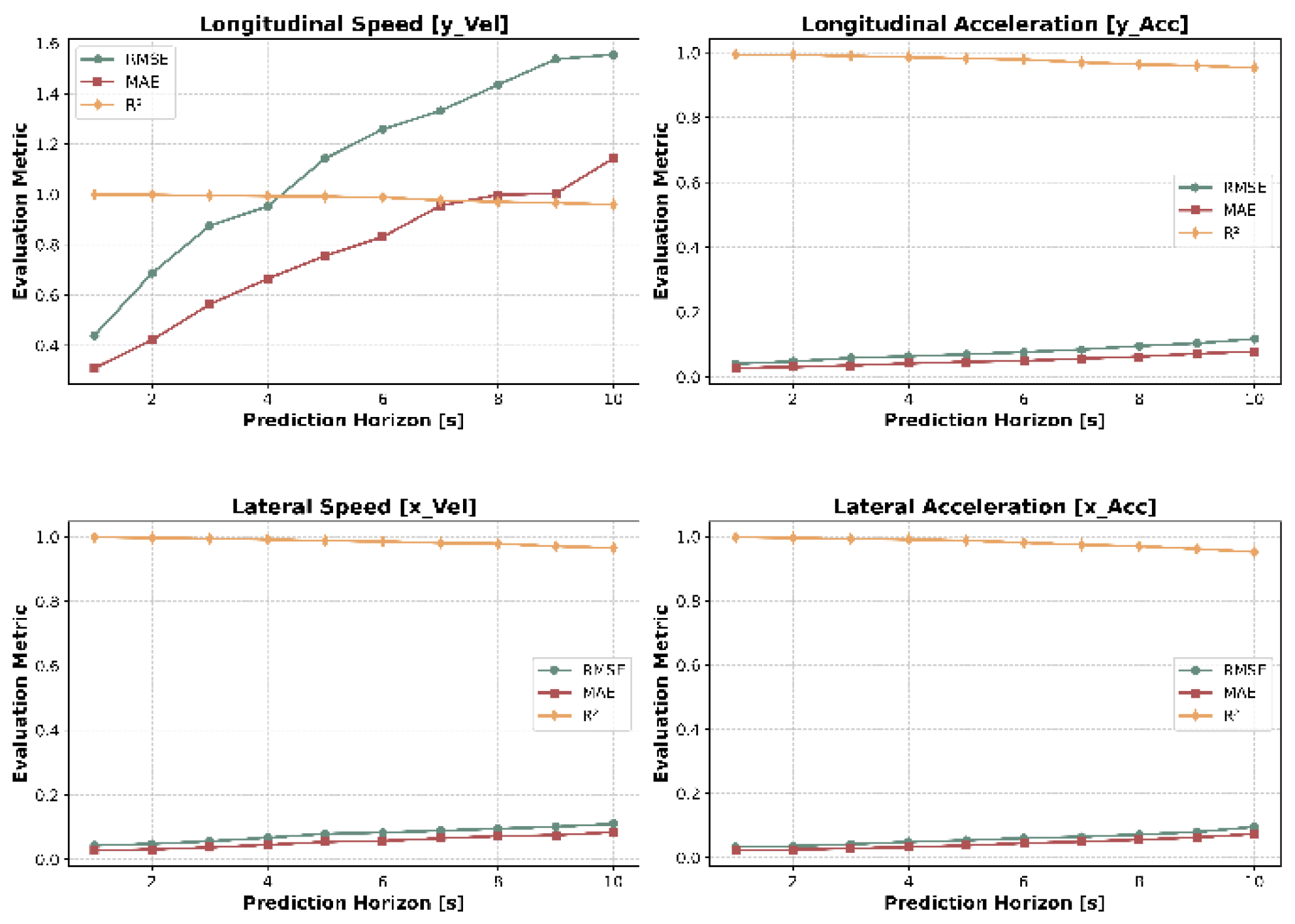
In this section, the HTSA-LSTM model is employed to predict the longitudinal speed (), longitudinal acceleration (), lateral speed (), and lateral acceleration () of vehicles. The same evaluation metrics used for trajectory prediction are applied here to assess the accuracy of the predictions. Figure 16, Figure 17 and Figure 18 present the prediction results for the target vehicle's various feature variables on CRS roads, UES roads, and HS roads, respectively.
Figure 16.
Prediction results for speed and acceleration on urban city roads (CRS).
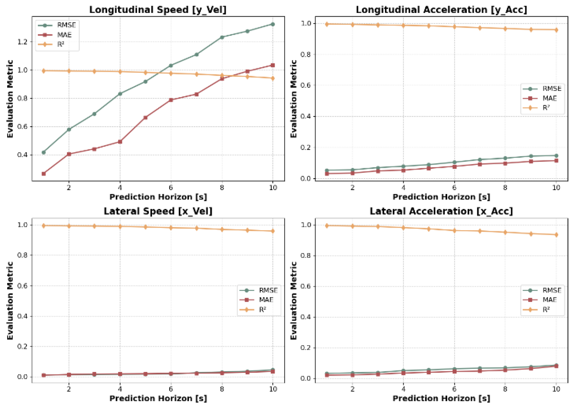
Figure 17.
Prediction results for speed and acceleration on urban city roads (UES).
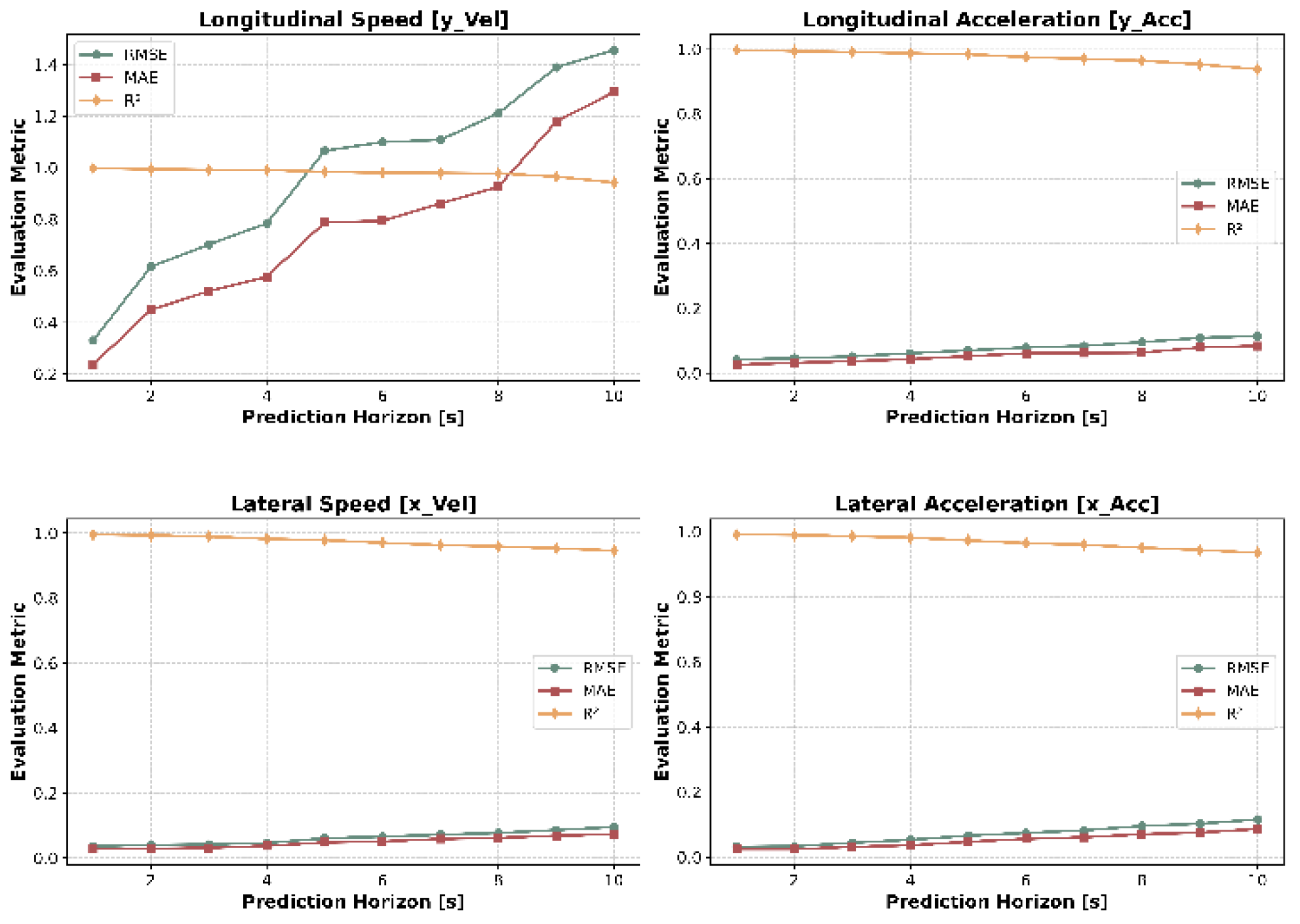
Figure 18.
Prediction results for speed and acceleration on urban city roads (HS).
5. Conclusions
Driving style analysis and vehicle trajectory prediction are critical for advancing intelligent vehicle technologies. This study examines variations in driving styles and introduces an innovative trajectory prediction model, HTSA-LSTM. The model is based on Long Short-Term Memory (LSTM) networks, integrating spatiotemporal attention mechanisms and driver behavior characteristics to achieve high-precision, long-term predictions. The key findings of this research are summarized as follows:
The study focuses on long-term vehicle trajectory prediction in multi-vehicle interaction scenarios. The HTSA-LSTM model incorporates a spatiotemporal attention mechanism to capture the complex spatiotemporal dependencies between vehicles. In addition to considering the continuity of vehicle motion and the influence of neighboring vehicles, the model segments driving data into driving primitives to analyze individual driving preferences, enabling precise future trajectory prediction. A 3×13 road grid structure was employed to represent the trajectories of the target vehicle and surrounding vehicles, and temporal and spatial attention weights were analyzed to identify key influential factors.
The model was trained and tested using the NGSIM US101 dataset, demonstrating a 20.72% reduction in RMSE and a 24.98% reduction in NLL for 5-second predictions compared to baseline models. The real-world applicability of HTSA-LSTM was validated using driving datasets, achieving over 97.9% accuracy for 5-second predictions on urban expressways (UES) and highways (HS), and 92.7% accuracy for 3-second predictions on city roads (CRS). Compared to STA-LSTM, HTSA-LSTM demonstrated superior prediction accuracy, especially in long-term forecasts (e.g., 6 seconds), with significantly lower RMSE and NLL metrics. This indicates that HTSA-LSTM exhibits greater robustness and accuracy in dynamic driving scenarios, showing clear advantages in handling vehicle interactions and complex environments, making it a promising solution for intelligent driving applications.
Author Contributions
Conceptualization, Y.W. and H.Z.; methodology, Y.W., X.Z, Z.L. H.W. and B.J.; software, X.Z, Z.L., X.C. and B.J; validation, X.C. and Z.Y.; formal analysis, Z.Y. and X.C.; investigation, Y.W., X.Z, Z.L. and B.J.; resources, Y.W. and H.W.; data curation, Z.Y., X.Z, Z.L. and B.J.; writing—original draft preparation, Y.W., X.Z, Z.L. and B.J.; writing—review and editing, Y.W.; visualization, X.C. and Z.Y.; supervision, Y.W.; project administration, Y.W.; funding acquisition, Y.W. All authors have read and agreed to the published version of the manuscript.
Funding
This research was funded by National Key Research and Development Project, grant number 2021YFC3001502.
Institutional Review Board Statement
Not applicable.
Informed Consent Statement
Not applicable.
Data Availability Statement
The data that support the findings of this study are available from the corresponding author, [Yiying.wei@whut.edu.cn], upon reasonable request. The data are not publicly available due to privacy.
Conflicts of Interest
The authors declare no conflicts of interest.
References
- Xing, Y.; Lv, C.; Wang, H.; Wang, H.; Ai, Y.; Cao, D.; Velenis, E.; Wang, F.-Y. Driver Lane Change Intention Inference for Intelligent Vehicles: Framework, Survey, and Challenges. IEEE Trans. Veh. Technol. 2019, 68, 4377–4390. [CrossRef]
- Messaoud, K., Yahiaoui, I., Verroust-Blondet, A., & Nashashibi, F. Relational recurrent neural networks for vehicle trajectory prediction. In Proceedings of the IEEE International Conference on Intelligent Transportation Systems (ITSC), Auckland, New Zealand, 27-30 October 2019; pp. 1813–1818. [CrossRef]
- Messaoud, K., Yahiaoui, I., Verroust-Blondet, A., & Nashashibi, F. Attention based vehicle trajectory prediction. IEEE Transactions on Intelligent Vehicles 2020, 6(1), 1–10. [CrossRef]
- Cao, D.; Wang, X.; Li, L.; Lv, C.; Na, X.; Xing, Y.; Li, X.; Li, Y.; Chen, Y.; Wang, F.-Y. Future Directions of Intelligent Vehicles: Potentials, Possibilities, and Perspectives. IEEE Trans. Intell. Veh. 2022, 7, 7–10. [CrossRef]
- Wang, L.-L.; Chen, Z.-G.; Wu, J. Vehicle trajectory prediction algorithm in vehicular network. Wirel. Networks 2018, 25, 2143–2156. [CrossRef]
- Cui, H., Radosavljevic, V., Chou, F. C., Lin, T. H., Thi, N., & Huang, T. K. Multimodal trajectory predictions for autonomous driving using deep convolutional networks. In Proceedings of the IEEE International Conference on Robotics and Automation (ICRA), Montreal, QC, Canada, 20-24 May 2019; pp. 2090–2096. [CrossRef]
- Choi, S.; Kim, J.; Yeo, H. Attention-based Recurrent Neural Network for Urban Vehicle Trajectory Prediction. Procedia Comput. Sci. 2019, 151, 327–334. [CrossRef]
- Xue, H.; Huynh, D.Q.; Reynolds, M. PoPPL: Pedestrian Trajectory Prediction by LSTM With Automatic Route Class Clustering. IEEE Trans. Neural Networks Learn. Syst. 2020, 32, 77–90. [CrossRef]
- Qian, L.P.; Feng, A.; Yu, N.; Xu, W.; Wu, Y. Vehicular Networking-Enabled Vehicle State Prediction via Two-Level Quantized Adaptive Kalman Filtering. IEEE Internet Things J. 2020, 7, 7181–7193. [CrossRef]
- Huang, Y.; Du, J.; Yang, Z.; Zhou, Z.; Zhang, L.; Chen, H. A Survey on Trajectory-Prediction Methods for Autonomous Driving. IEEE Trans. Intell. Veh. 2022, 7, 652–674. [CrossRef]
- Polychronopoulos, A.; Tsogas, M.; Amditis, A.J.; Andreone, L. Sensor Fusion for Predicting Vehicles' Path for Collision Avoidance Systems. IEEE Trans. Intell. Transp. Syst. 2007, 8, 549–562. [CrossRef]
- Jin, B.; Jiu, B.; Su, T.; Liu, H.; Liu, G. Switched Kalman filter-interacting multiple model algorithm based on optimal autoregressive model for manoeuvring target tracking. IET Radar, Sonar Navig. 2015, 9, 199–209. [CrossRef]
- Matthias, A., & Alexander, M. Comparison of Markov Chain Abstraction and Monte Carlo Simulation for the Safety Assessment of Autonomous Cars. IEEE Transactions on Intelligent Transportation Systems 2011, 12(4), 1237-1247.
- Bahram, M.; Hubmann, C.; Lawitzky, A.; Aeberhard, M.; Wollherr, D. A Combined Model- and Learning-Based Framework for Interaction-Aware Maneuver Prediction. IEEE Trans. Intell. Transp. Syst. 2016, 17, 1538–1550. [CrossRef]
- Zhu, X.; Hu, W.; Deng, Z.; Zhang, J.; Hu, F.; Zhou, R.; Li, K.; Wang, F.-Y. Interaction-Aware Cut-In Trajectory Prediction and Risk Assessment in Mixed Traffic. Ieee/caa J. Autom. Sin. 2022, 9, 1752–1762. [CrossRef]
- Ho, J., & Ermon, S. Generative Adversarial Imitation Learning. In Proceedings of the 30th Annual Conference on Neural In-formation Processing Systems (NIPS), Barcelona, Spain, 5-10 December 2016; p. 19.
- Choi, S.; Kim, J.; Yeo, H. TrajGAIL: Generating urban vehicle trajectories using generative adversarial imitation learning. Transp. Res. Part C: Emerg. Technol. 2021, 128. [CrossRef]
- Tang, C., & Salakhutdinov, R. R. Multiple futures prediction. Advances in Neural Information Processing Systems 2019, 32, 15424-15434.
- Liu, Y. C., Zhang, J. H., Fang, L. J., et al. Multimodal Motion Prediction with Stacked Transformers. In Proceedings of the IEEE/CVF Conference on Computer Vision and Pattern Recognition, Nashville, TN, USA, 19-25 June 2021; pp. 7577-7586.
- Li, M., Tong, P., & Li, M. Traffic flow prediction with vehicle trajectories. In Proceedings of the AAAI Conference on Artificial Intelligence, Vancouver, BC, Canada, 2-9 February 2021; 35(1), 294-302.
- Jo, E.; Sunwoo, M.; Lee, M. Vehicle Trajectory Prediction Using Hierarchical Graph Neural Network for Considering Interaction among Multimodal Maneuvers. Sensors 2021, 21, 5354. [CrossRef]
- Li, R. N., Qin, Y., Wang, J. B., et al. AMGB: Trajectory prediction using attention-based mechanism GCN-BiLSTM in IOV. Pattern Recognition Letters 2023, 169, 17-27.
- Mo, X.; Huang, Z.; Xing, Y.; Lv, C. Multi-Agent Trajectory Prediction With Heterogeneous Edge-Enhanced Graph Attention Network. IEEE Trans. Intell. Transp. Syst. 2022, 23, 9554–9567. [CrossRef]
- Shi, J.; Sun, D.; Guo, B. Vehicle Trajectory Prediction Based on Graph Convolutional Networks in Connected Vehicle Environment. Appl. Sci. 2023, 13, 13192. [CrossRef]
- Li, H.; Ren, Y.; Li, K.; Chao, W. Trajectory Prediction with Attention-Based Spatial–Temporal Graph Convolutional Networks for Autonomous Driving. Appl. Sci. 2023, 13, 12580. [CrossRef]
- Ni, Q.; Peng, W.; Zhu, Y.; Ye, R. A Novel Trajectory Feature-Boosting Network for Trajectory Prediction. Entropy 2023, 25, 1100. [CrossRef]
- Lin, L.; Li, W.; Bi, H.; Qin, L. Vehicle Trajectory Prediction Using LSTMs With Spatial–Temporal Attention Mechanisms. IEEE Intell. Transp. Syst. Mag. 2021, 14, 197–208. [CrossRef]
- Nachiket, D., & Mohan, M. T. Convolutional Social Pooling for Vehicle Trajectory Prediction. In Proceedings of the IEEE Conference on Computer Vision and Pattern Recognition Workshops (CVPRW), Salt Lake City, UT, USA, 18-22 June 2018; pp. 1468-1476.
- Robert, C. M. On Log-Likelihood-Ratios and the Significance of Rare Events. In Proceedings of the 2004 Conference on Empirical Methods in Natural Language Processing (EMNLP), Barcelona, Spain, 25-26 July 2004; pp. 333-340.
- Wei, Y. , Jia, B. , Xiao, X. , & Yao, B. Driving style analysis in car-following scenarios based on semantic analysis method. 2023 7th CAA International Conference on Vehicular Control and Intelligence (CVCI). [CrossRef]
- Samer, A., & Fawzi, N. Real time trajectory prediction for collision risk estimation between vehicles. In Proceedings of the 2009 IEEE 5th International Conference on Intelligent Computer Communication and Processing (ICCP), Cluj-Napoca, Romania, 27-29 August 2009; pp. 417-422. [CrossRef]
- Alex, Z., Stewart, W., James, W., et al. Long Short Term Memory for Driver Intent Prediction. In Proceedings of the 2017 IEEE Intelligent Vehicles Symposium (IV), Los Angeles, CA, USA, 11-14 June 2017; pp. 1484-1489. [CrossRef]
- Nachiket, D., & Mohan, M. T. Multi-Modal Trajectory Prediction of Surrounding Vehicles with Maneuver based LSTMs. In Proceedings of the 2018 IEEE Intelligent Vehicles Symposium (IV), Changshu, China, 26-30 June 2018; pp. 1179-1184. [CrossRef]
- Kaouther M, Itheri Y, Anne V B, et al. Attention Based Vehicle Trajectory Prediction[J]. IEEE Transactions on Intelligent Vehicles, 2021, 6(1): 175-185. [CrossRef]
- Qi, G.; Du, Y.; Wu, J.; Xu, M. Leveraging longitudinal driving behaviour data with data mining techniques for driving style analysis. IET Intell. Transp. Syst. 2015, 9, 792–801. [CrossRef]
Figure 1.
Discretization of the road network space into a 3×13 grid.
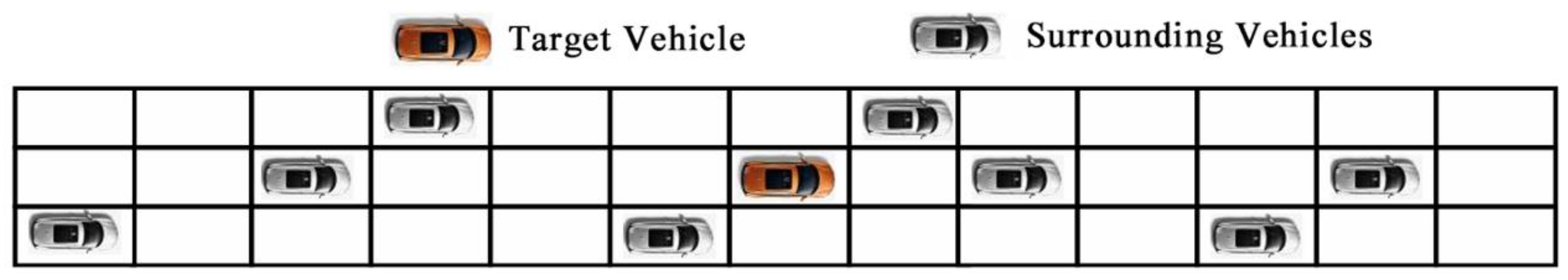
Figure 2.
the traditional LSTM architecture.
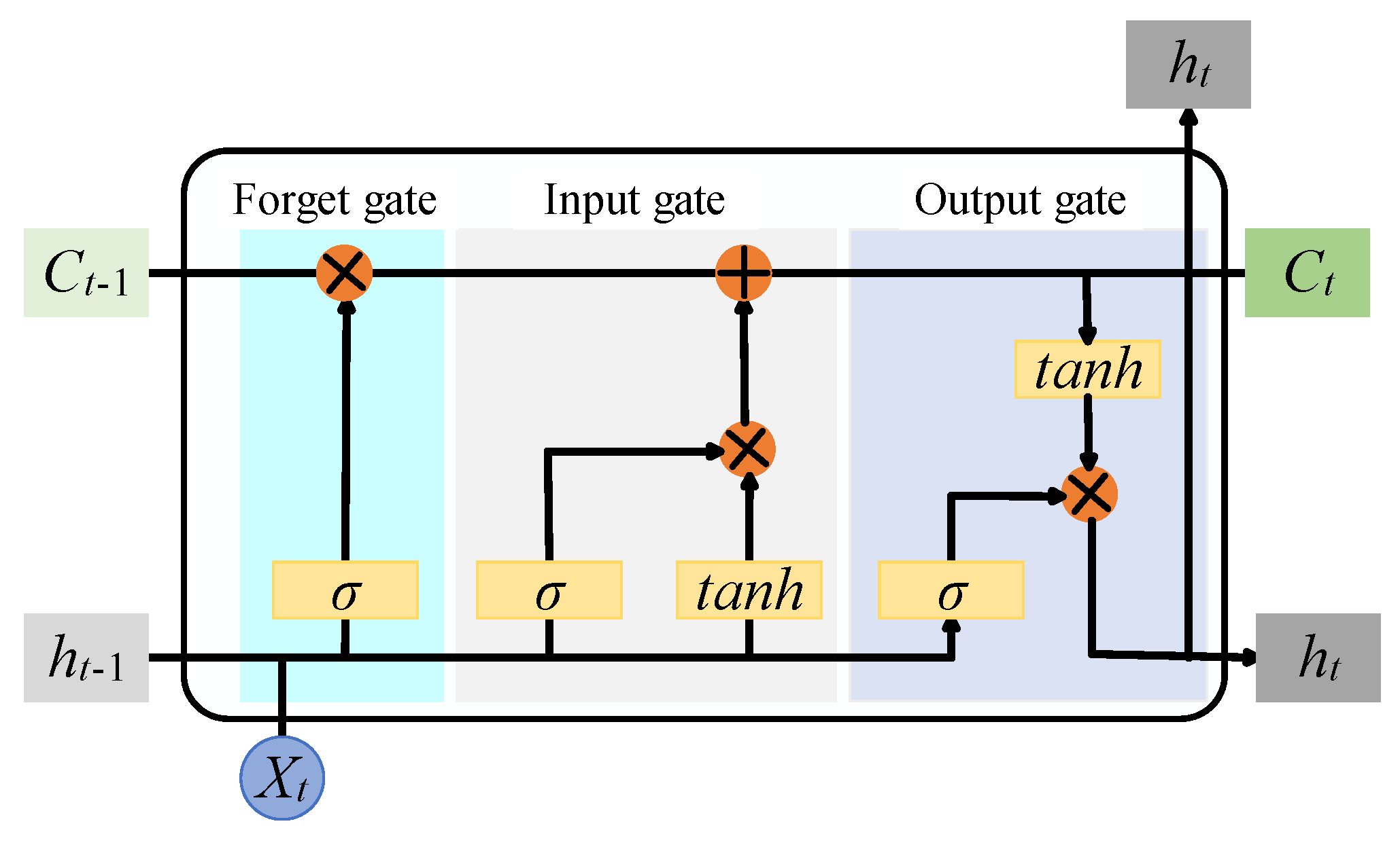
Figure 3.
The integration module of driving styles analyze.
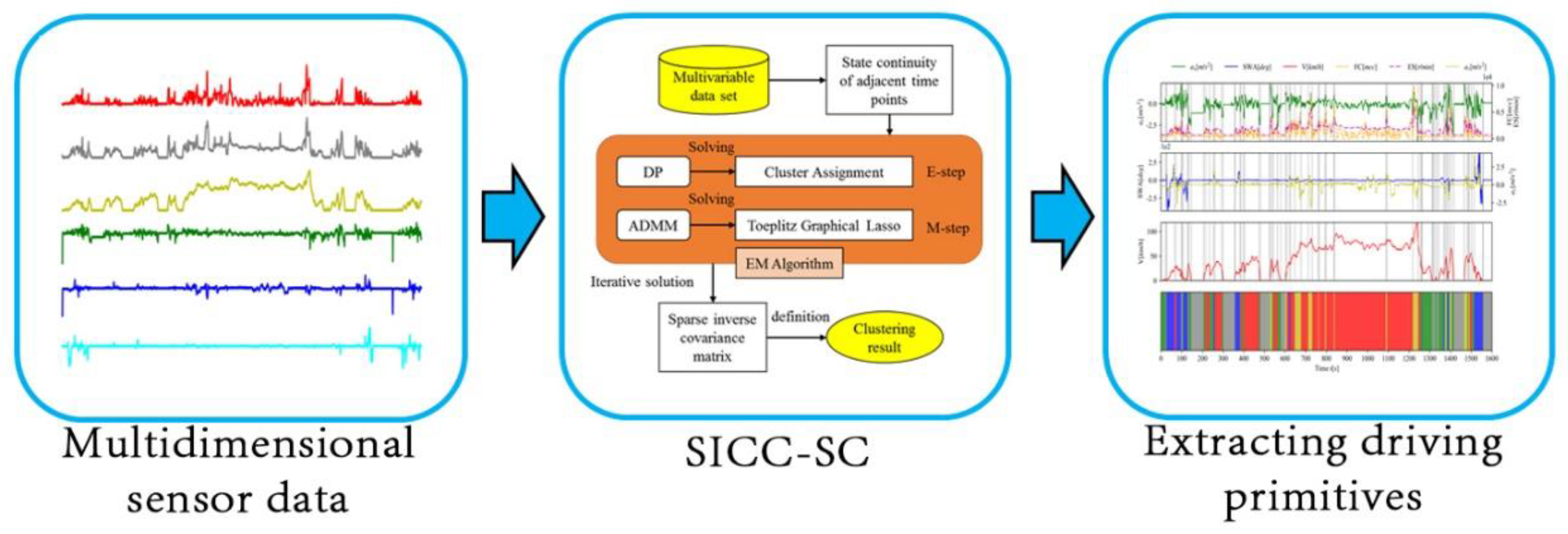
Figure 4.
HTSA-LSTM model diagram.
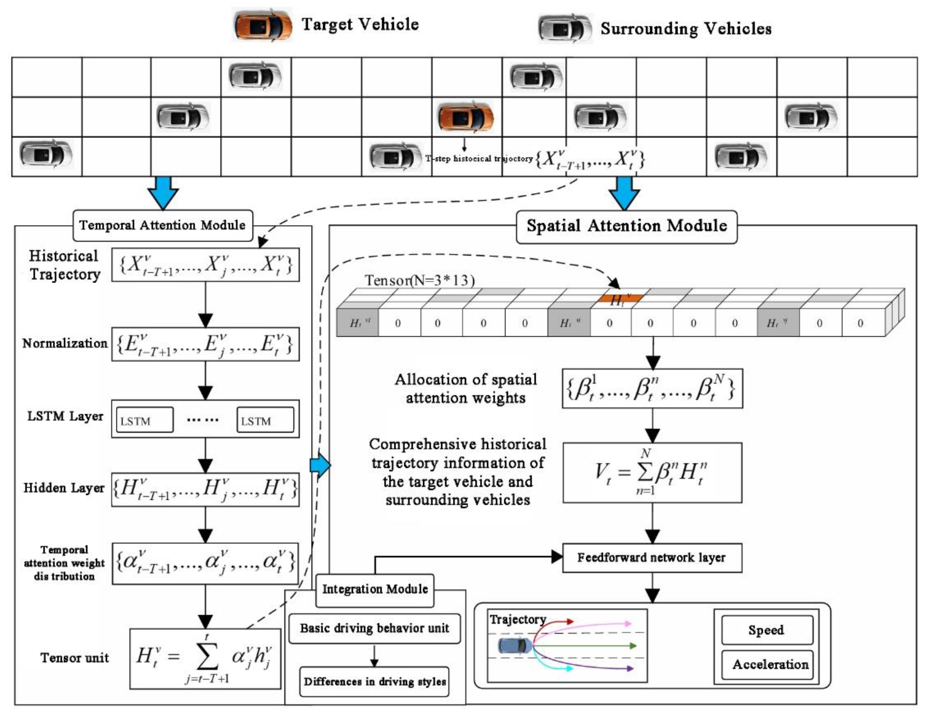
Figure 5.
The data segmentation process.
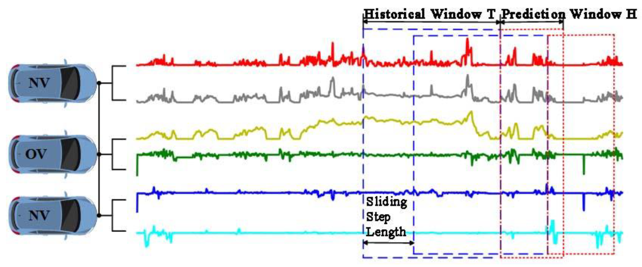
Figure 6.
The distribution of temporal attention.
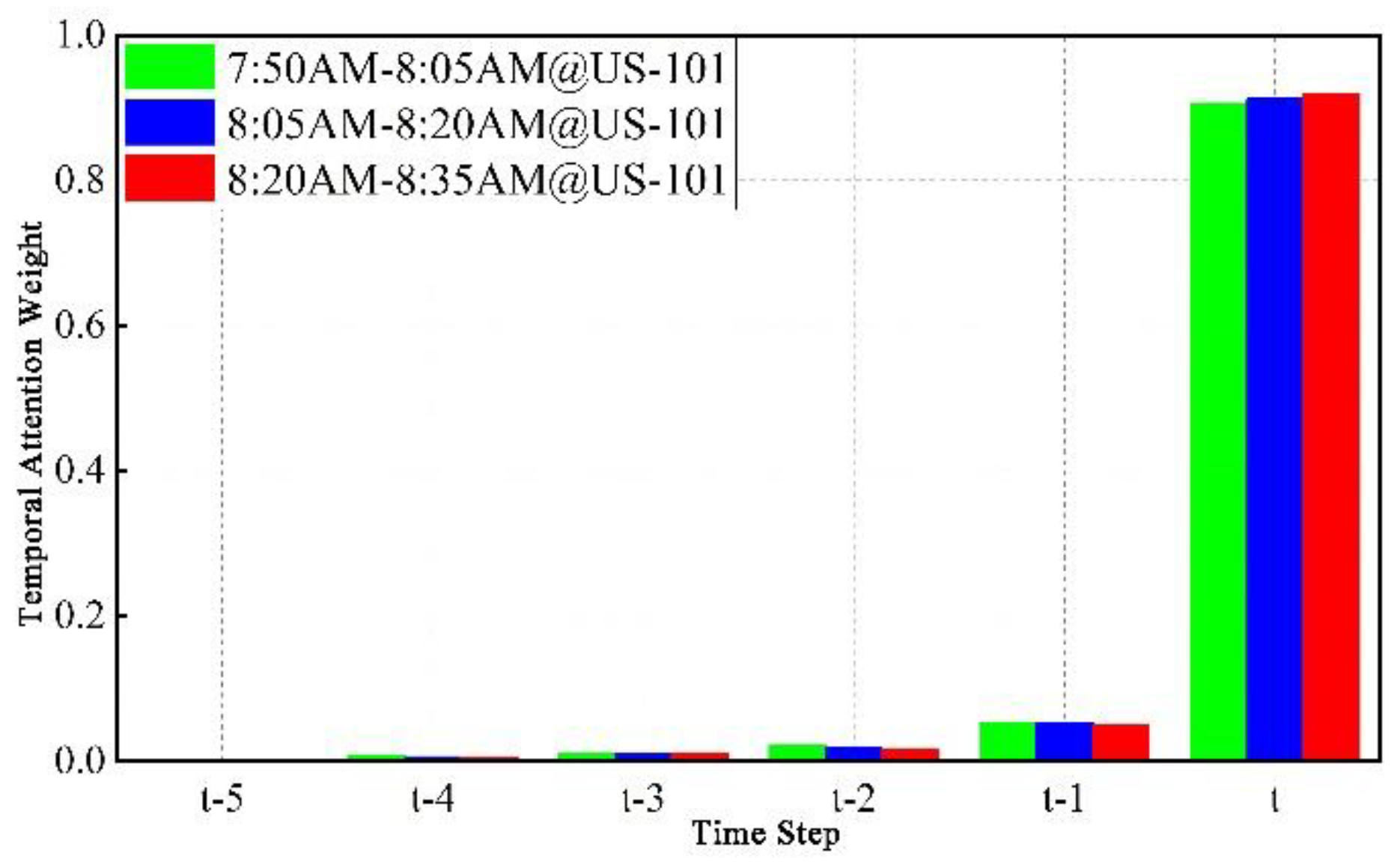
Figure 7.
The lane distribution at the Ventura Boulevard on-ramp.
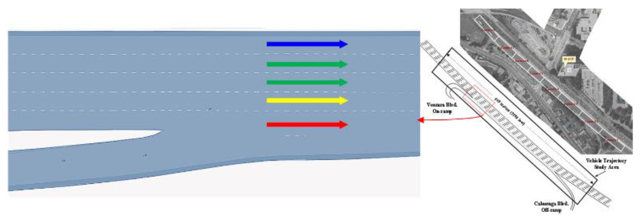
Figure 8.
Spatial attention allocation
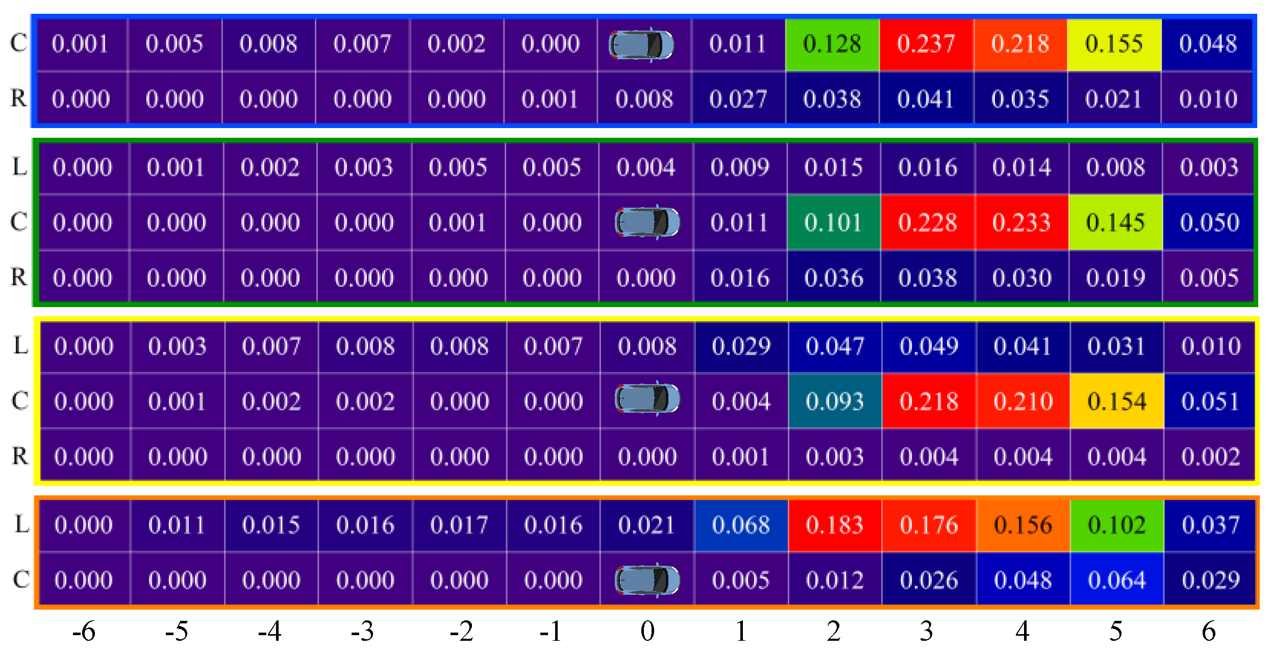
Figure 9.
Spatial attention shift during lane change for vehicle 1585
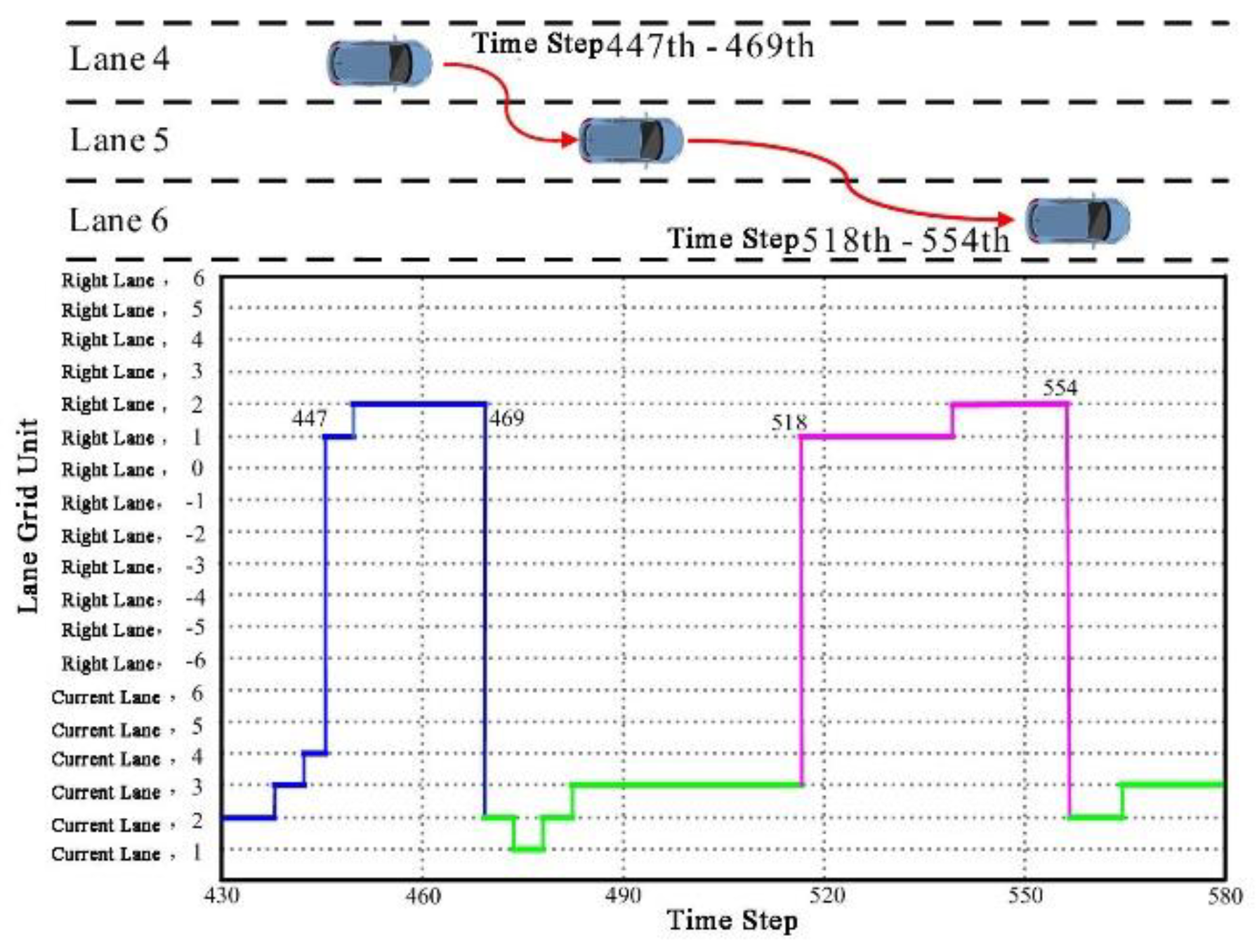
Figure 10.
Driving behavior and kinematic features
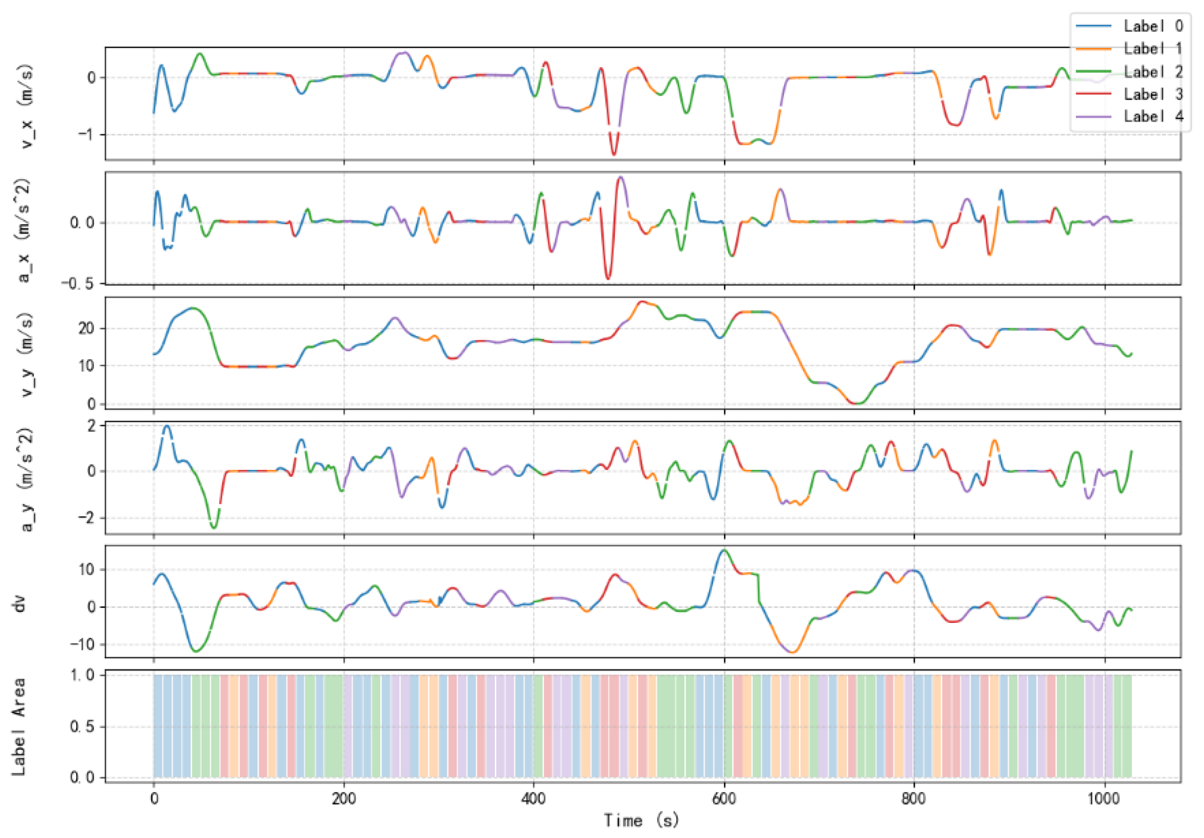
Figure 11.
Standardized frequency distribution of driving primitives.
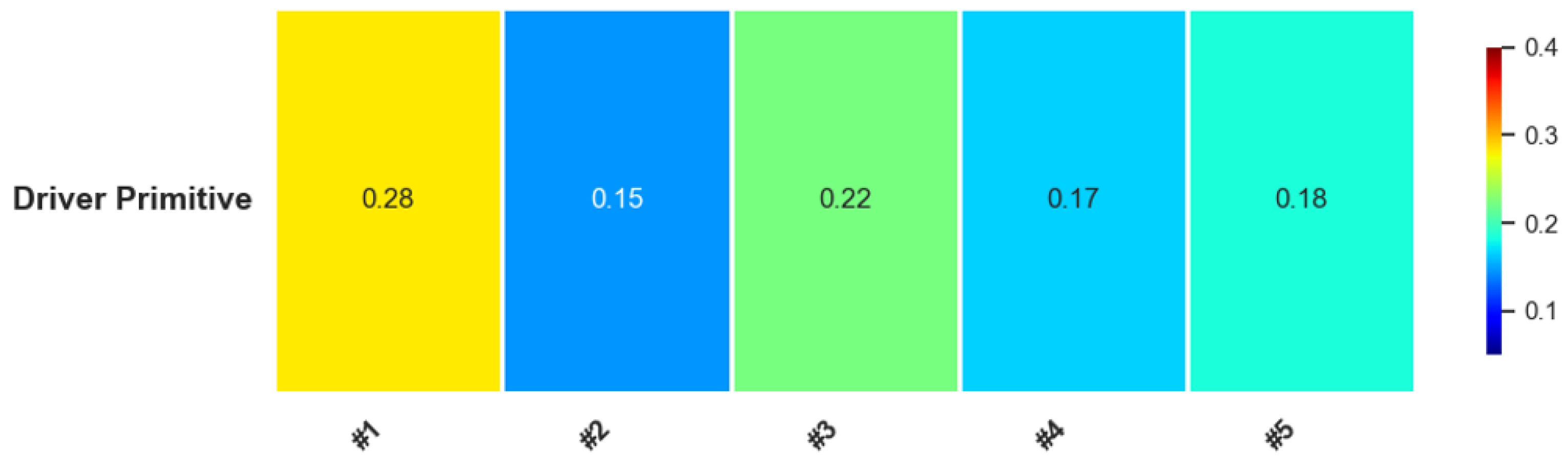
Figure 12.
Examples of predictions for vy, ay, vx ,ax for Vehicle 1585 (with H=5 and H=8).
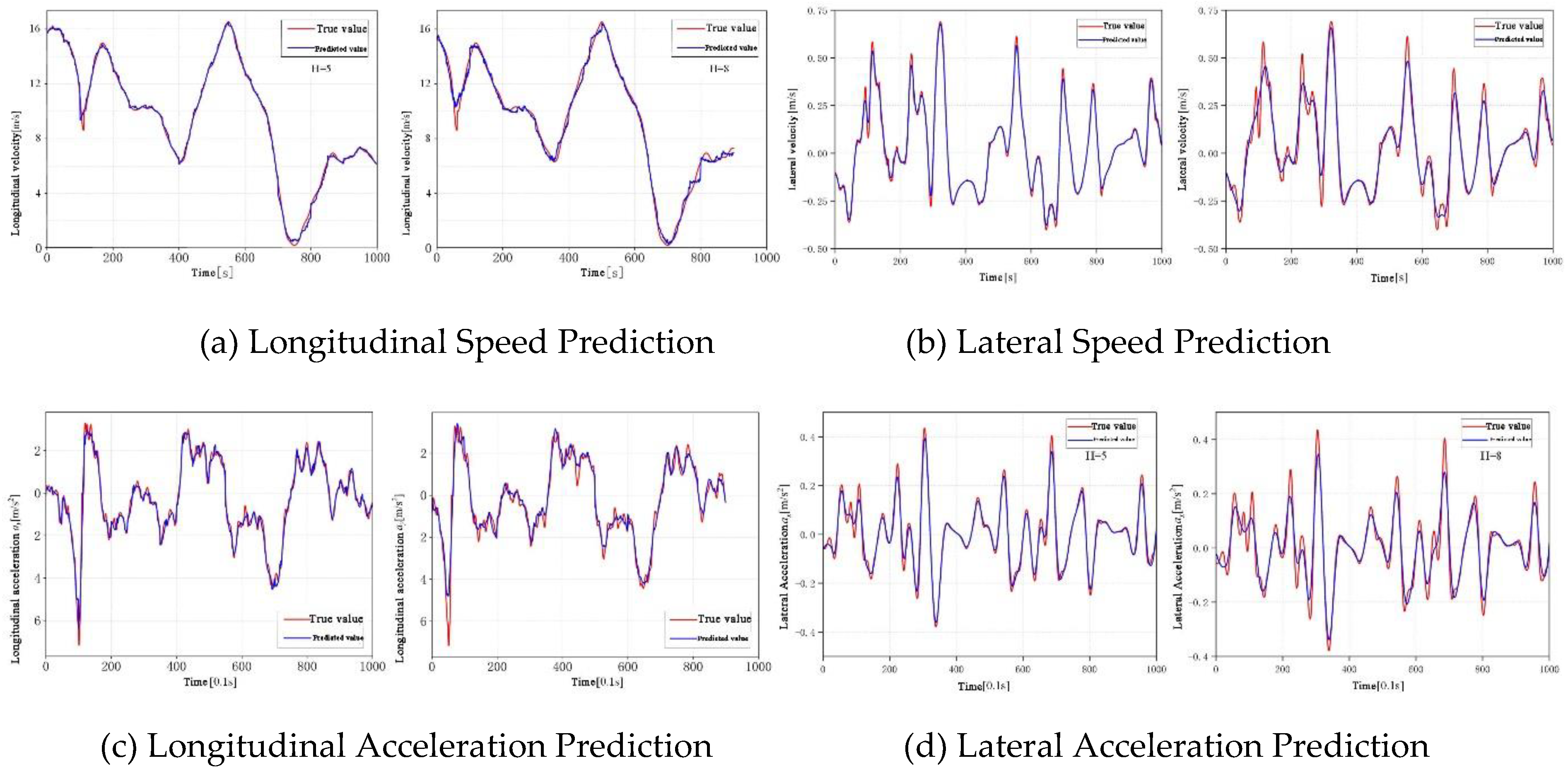
Figure 13.
Shows the relationship between , , , , and the prediction horizon.
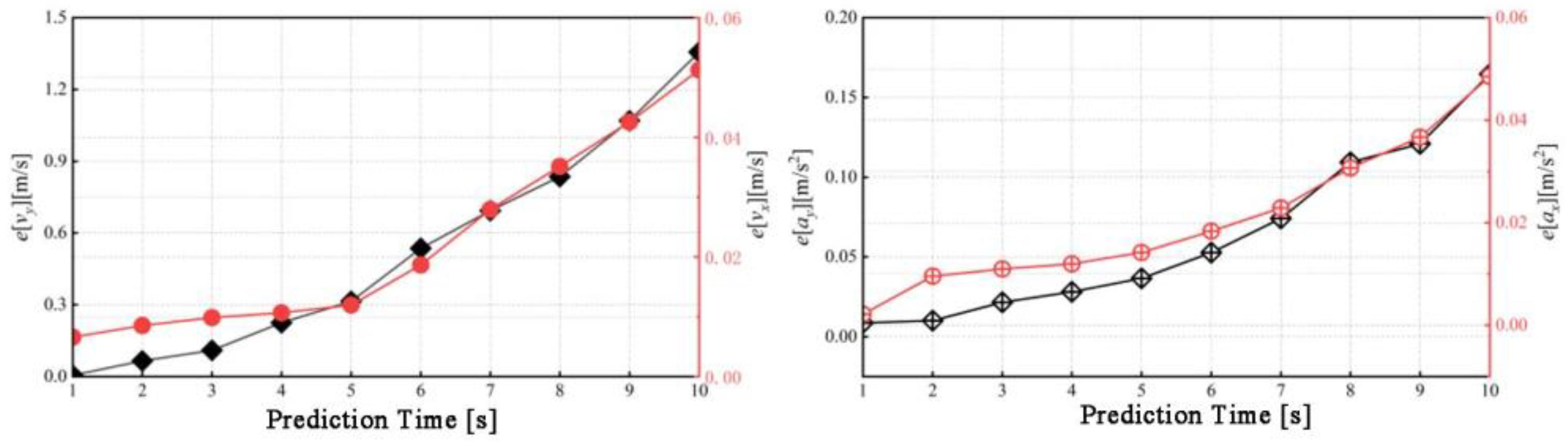
Figure 14.
Shows the trajectory predictions for vehicle 1585 and its neighboring vehicles.
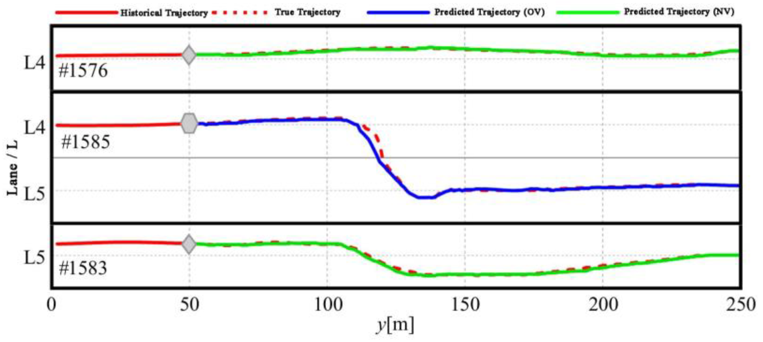
Figure 15.
experimental routes.
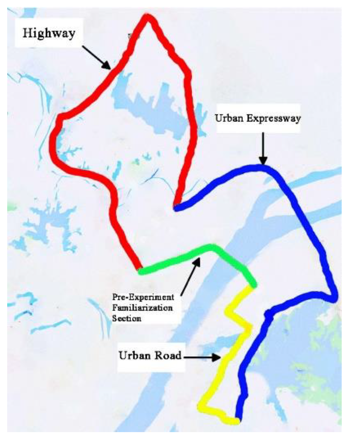
Table 2.
Hyperparameter list of the model.
| Parameter | Value |
|---|---|
| Input layer dimension of LSTM encoder | 32 |
| Dimension of LSTM hidden vectors | 64 |
| Feedforward network layer dimension | 128 |
| Input data (grid_size: 3×13 road network structure) | 13,3 |
| Batch size | 128 |
| Learning rate (Lr) | 0.001 |
| Optimizer | Adam |
| Training epochs | 200 |
| 2 | |
| 0.11 | |
| 15 | |
| 35 | |
| 5 |
Table 3.
Shows the evaluation metrics of the models over a 6-second prediction horizon.
| Evaluation Metric | Prediction Duration [s] | CV | S-LSTM | M-LSTM | A-LSTM | CS-LSTM | STA-LSTM | HTSA-LSTM |
|---|---|---|---|---|---|---|---|---|
| RMSE | 1 | 0.953 | 0.683 | 0.584 | 0.648 | 0.623 | 0.615 | 0.499 |
| 2 | 1.826 | 1.538 | 1.263 | 1.325 | 1.268 | 1.256 | 0.898 | |
| 3 | 3.352 | 2.466 | 2.128 | 2.163 | 2.065 | 2.047 | 1.314 | |
| 4 | 5.885 | 3.847 | 3.245 | 3.258 | 3.137 | 3.044 | 2.225 | |
| 5 | 8.943 | 5.236 | 4.661 | 4.562 | 4.366 | 4.281 | 3.461 | |
| 6 | 11.127 | 6.542 | 6.157 | 6.037 | 5.879 | 5.761 | 4.897 | |
| NLL | 1 | 3.718 | 2.023 | 1.173 | 1.012 | 0.576 | 0.630 | 0.603 |
| 2 | 5.372 | 3.634 | 2.851 | 2.487 | 2.142 | 1.088 | 1.115 | |
| 3 | 7.389 | 4.628 | 3.806 | 3.362 | 3.028 | 1.718 | 2.056 | |
| 4 | 9.164 | 5.352 | 4.479 | 4.158 | 3.692 | 2.735 | 2.769 | |
| 5 | 10.895 | 6.295 | 5.095 | 5.036 | 4.351 | 4.077 | 3.264 | |
| 6 | 12.026 | 7.036 | 6.432 | 6.347 | 6.028 | 5.852 | 4.318 |
Table 4.
HTSA-LSTM model performance on real-world driving data.
| Road Type | Prediction Horizon [s] | Evaluation Metrics | ||
|---|---|---|---|---|
| RMSE | MAE | R2 | ||
| CRS | 1 | 0.092 | 0.026 | 0.959 |
| 2 | 0.086 | 0.025 | 0.938 | |
| 3 | 0.103 | 0.037 | 0.927 | |
| 4 | 0.126 | 0.039 | 0.912 | |
| 5 | 0.114 | 0.054 | 0.895 | |
| 6 | 0.119 | 0.062 | 0.888 | |
| 7 | 0.132 | 0.067 | 0.872 | |
| 8 | 0.151 | 0.078 | 0.863 | |
| 9 | 0.172 | 0.093 | 0.859 | |
| 10 | 0.188 | 0.098 | 0.851 | |
| UES | 1 | 0.009 | 0.007 | 0.997 |
| 2 | 0.012 | 0.009 | 0.994 | |
| 3 | 0.017 | 0.013 | 0.991 | |
| 4 | 0.019 | 0.015 | 0.989 | |
| 5 | 0.021 | 0.016 | 0.980 | |
| 6 | 0.025 | 0.020 | 0.971 | |
| 7 | 0.031 | 0.024 | 0.962 | |
| 8 | 0.038 | 0.029 | 0.955 | |
| 9 | 0.042 | 0.031 | 0.947 | |
| 10 | 0.047 | 0.036 | 0.941 | |
| HS | 1 | 0.014 | 0.011 | 0.996 |
| 2 | 0.017 | 0.014 | 0.994 | |
| 3 | 0.021 | 0.017 | 0.991 | |
| 4 | 0.023 | 0.018 | 0.986 | |
| 5 | 0.032 | 0.026 | 0.979 | |
| 6 | 0.039 | 0.030 | 0.969 | |
| 7 | 0.042 | 0.033 | 0.957 | |
| 8 | 0.049 | 0.040 | 0.949 | |
| 9 | 0.057 | 0.048 | 0.944 | |
| 10 | 0.068 | 0.054 | 0.936 | |
Disclaimer/Publisher’s Note: The statements, opinions and data contained in all publications are solely those of the individual author(s) and contributor(s) and not of MDPI and/or the editor(s). MDPI and/or the editor(s) disclaim responsibility for any injury to people or property resulting from any ideas, methods, instructions or products referred to in the content. |
© 2025 by the authors. Licensee MDPI, Basel, Switzerland. This article is an open access article distributed under the terms and conditions of the Creative Commons Attribution (CC BY) license (http://creativecommons.org/licenses/by/4.0/).
Copyright: This open access article is published under a Creative Commons CC BY 4.0 license, which permit the free download, distribution, and reuse, provided that the author and preprint are cited in any reuse.


