Submitted:
11 January 2025
Posted:
13 January 2025
Read the latest preprint version here
Abstract
It is generally assumed that information about the exact nature of truly random events can only be obtained after those events occur. One empirical apparent contradiction of this assumption is the causally ambiguous duration-sorting (CADS) effect, in which photon absorptions are measured before a truly random decision about the duration of an experiment is made. The only parameter varied across experimental runs is the duration between on- and off-times, yet the number of photons absorbed prior to this decision is related to the decision itself. This report focuses on further examining the CADS effect by characterizing the pre-decision periods for data continuously recorded for 365 days in an independent laboratory using upgraded equipment. A complex but reliable periodicity gave a conservative estimate of 4.7 for sigma, and a linear CADS equation emerged to estimate magnitude at peak frequencies for each of four equiprobable post-decision durations. An apparently novel relationship between photon absorptions and lunar phase was also found. Determining whether accurate pre-decision information about future durations is only available in retrospect requires further experimentation, but these results strongly support apparent retrocausality or at least causal ambiguity in groups of photons with shared classical boundaries in time.

Keywords:
retrocausality
; time symmetry
; ambiguous causality
; superdeterminism
; post-selection
; acausality
; photonics
; moon
; quantum computing
; metrology
; precision timing
1. Introduction
Several physical effects, such as delayed-choice experiments and inhibited spontaneous emission, can be explained using retrocausality – the idea that seemingly future effects in some way influence present events [1,2,3,4,5,6,7,8]. Recently, advances in empirical approaches to demonstrating retrocausal effects have also emerged in the quantum computing space. For one example, an apparent “backwards in time” manipulation of entangled quantum bits (qubits) allows the “future” qubit to inform the choice of initial state of the “past” qubit [9,10]. The motivation for such an experiment is at least partially derived from the idea that the well-known “quantum speedup” making quantum computing so desirable is in fact due to retrocausation [11,12]. However, most quantum computing technology currently relies on isolating atoms, ions, and photons from decohering effects [13]. If there were a way to obtain temporally nonlocal, or retrocausal effects with groups of photons at room temperature, this would positively impact the design of quantum computers that harness temporally nonlocal, acausal, or retrocausal phenomena. More importantly, if such effects could be demonstrated easily at room temperature and without the use of metamaterials, this would support wider experimentation in quantum electrodynamics and quantum mechanics in general. These and other motivations have led to this report, which aims to further characterize one such easily demonstrated apparently retrocausal effect called CADS (Causally Ambiguous Duration Sorting). The initial CADS pilot experiment [14] demonstrated the effect and the follow-up white paper [15] named it CADS. CADS was named after the primary observation, which was that experimental runs with different durations on the seconds-to-minutes time scale could be distinguished by differences in photon absorption counts recorded prior to a truly random decision about the duration of the experimental run.
Although the mechanism remains unknown, a CADS hypothesis emerged from these experiments. Specifically, the hypothesis is that the classical on-off boundaries of an optical experiment entangle photons considered to be included within those boundaries, consistent with a non-dynamical picture [16]. However, the original experiments used sub-standard equipment that had a tendency to fail. Further, the random number generator used to make the decision about the future duration of the experimental run drew randomness from the odd- or evenness- of the photon counts recorded prior to this decision, so while this source of randomness was truly random, it could be considered to be entangled with the photons themselves and therefore the interpretation became complicated. Further, in those experiments the equipment was housed in the home of the experimenter and could not be run at night due to noise, so the effect was only measured during the day. Finally, in those experiments, some periodicities in the direction of the effect were qualitatively observed [15] but could not be investigated quantitatively without continuous data gathering.
Physicist Winthrop Williams volunteered to build an independent system to perform a year-long continuous CADS experiment. After analyzing data from the first half-year, he presented his results at a conference but did not continue to pursue the effect because he was primarily interested in replicating the overall effect that was not dependent on complex periodicities [17]. However, Williams generously offered his entire data set to the author for additional analysis, and this report is entirely based on those data.
2. Materials and Methods
Protocol
The protocol for the Williams & Mossbridge [17] replication was the same as the initially described CADS effect for experiments 1, 2, and 3 [15] except where noted here. Briefly, in both experiments, a non-laser light source was used to emit light and a detector was used to count photon absorptions within 11-s observation windows. The parameter varied across experimental runs was the duration between the on- and off-times of the emitter and detector (referred to as “the optics”). This duration was randomly selected from four equiprobable durations after the optics had already been turned on and three observations had already been recorded. The possible post-decision observations were designed to be: 0 observations (the optics were immediately turned off), 20 observations (the optics were turned off after 220 s), 30 observations (the optics were turned off after 330 s), and 60 observations (the optics were turned off after 660 s). Immediately after the optics were turned off, the 180-s inter-run interval began (Figure 1).
In the year-long replication [17], an additional 6 s were required to warm up the optics prior to each run, and it was found empirically that each run was an average of 3.199978 s +/- 0.8 s longer than intended. Thus one run of the replication, including the 180-s inter-run interval, took 222.2 s (0 post-decision observations, total seconds of observation = 33 s [pre-decision observations only]), 442.2 s (20 post-decision observations, total seconds of observation = 253), 552.2 s (30 post-decision observations, total seconds of observation = 363), or 882.2 s (60 post-decision observations, total seconds of observation = 693). Further, the entire experiment was run continuously for a year, from July 27, 2020 to July 27, 2021, and each run was timestamped. In comparison, the original three experiments with the same protocol comprised data gathered only during daytime, derived from three 10-day periods [15].
Equipment
Optics. The desire was to attenuate photons reaching the detector as the original effect had been found at relatively low counting rates. The optics were encased in a black box. The light source was a red (~650 nm) light-emitting diode (LED) that was diffused (via Magic Scotch tape) and attenuated by an infrared (~880 nm) de-tuned bandpass filter. The photons coupled in a fiber coupler were sent to the detector, a single-photon counting module (i.e., a reverse-bias diode). Average count rate was about 3000 counts per s.
Input/Output and Control. Pulses from the detector were counted by an independent field programmable gate array (FPGA), and the counts over each 11-s observation window were summed and recorded by the controlling Labview software. The onset and offset times of the optics were controlled by Labview, which informed the resistor-capacitor (RC) circuit used for ramping the voltage up and down. This RC circuit was optically isolated from the computer to avoid ground loops.
Random Number Generation. A breadboard (i.e. discrete logic) implementation of an 80-bit shift register pseudorandom number generator clocked by independent photomultiplier pulses generated by a tank of scintillator oil was used to instantiate a completely independent, non-computer based hardware random number generator. Flashes of light in the scintillator oil were converted to electrical pulses using a photomultiplier, with output sent through an amplifier and threshold discriminator. To make the four potential post-decision durations equiprobable, these truly random pulses were used as the clock inputs on 10 CD4015 CMOS ICs circuits. Each time there was a detection in the scintillator oil tank, the circuit board advanced to the next pseudorandom number. The pseudorandom sequence repeated every 280-1 clocks. The approximate 40 Hz pulse rate of the scintillator oil provided a fresh 80 bits every 2 s. Two of these bits were collected by the Labview system via two jumper wires connecting to the circuit board with the 80-bit shift register.
Laboratory Environment. The replication was performed in a small room next to the Berkeley Advanced Physics lab which was seldom entered by Williams during the course of the year-long replication and was never entered by others. The room had one window with shades drawn and the space was climate controlled.
Data Analysis
Dependent Variables. Once the third photon count was recorded, the decision was made by the control software using input from the random number generator. To characterize the CADS effect, the primary dependent variable was the arithmetic value of the summed photon counts in the first three 11-s observation bins, prior to the duration decision. At no time were post-decision photon counts analyzed for this report (for discussion of post-decision counts for the first half of this data set, see [17]. Other dependent variables described in this report are all derivations from these pre-decision means, except when the entire signal was used for high-pass filtering. No outliers were removed, but see (Methods: Examining Periodicities) for an explanation of the removal of one 6-hour windowed data point.
High-pass Filtering. There were long time-frame periodicities in the 11-Hz sampled time series data; these corresponded to 12-, 24- and longer periods (e.g., 25-32 days, Figure 2A). The effect of interest occurred at shorter time frames, and it was possible that these longer periodicities would make detecting that effect difficult, so Matlab was used to apply an exponential-ramp high-pass filter to the Fourier-obtained magnitudes. An inverse Fourier transform was used to check that the longer periodicities were indeed removed from the time series (Figure 2B). A Fourier transform of the filtered data indicated that the filter attenuated periods of ~57 hours and above to 0, at periods of ~12-hours magnitudes were at 5.6% of the original values, and at ~4.6 hours they were completely unattenuated (Figure 3). The mean values used as dependent variables were calculated from the high-pass filtered time series, except where explicitly noted.
Calculating Lunar Phases. Because the period of one of the longer periodicities in the pre-filtered data was around the time of a lunar cycle (25-32 days), the pre-filtered time series data were examined to determine if there was any relationship between the mean pre-decision photon counts and the moon phases during the time the photon counts were gathered. To find the lunar phases for each experimental run, a modified Matlab interpretation of a Python script [18] was applied to the Unix date/time stamps for each run, converting Unix date/time stamps to nine lunar phases, with the new moon separated into two days.
Examining Periodicities in Pre-decision Means. A 6-hour duration of the time window for the periodicity analysis was selected for three reasons: 1) given the equiprobability of the post-decision durations, 6 hours would be enough time to contain around 10 instances of each of the post-decision durations, and 2) the post-filtered data showed no special peak at periods around 6 hours (Figure 3, red asterisk), so any fluctuation that differed between pre-decision means across post-decision durations would be easier to detect than if a natural peak existed at that period, and 3) the original CADS effect was obtained from data gathered in 5-to-6 hour windows each day [15]. The mean and standard deviations across all pre-decision means within each 6-hour window were calculated separately for each post-decision duration, providing 1460 6-hour means and standard deviations for each post-decision duration. One of these 6-hour time periods did not contain any durations that consisted of 20 observation windows, so data from that time period was deleted from all four post-decision duration datasets except preceding FFT analysis of the 6-hour-windowed time series data, below. To determine whether the observed periodicities were statistically reliable, the 6-hour means and standard deviations were used to calculate sigmas (as Z-scores derived from t-distributions) for comparisons of each of the 1459 windows between each of the four equiprobable post-decision durations, resulting in 1459 sigmas representing the absolute value of the effect for each post-decision duration comparison at each time window. To obtain sigmas for values that were incalculable, a sigma of 8.21 was artificially imposed by subtracting a very small value (1x10-16) from the probability density function.
FFT Analysis Per Post-Decision Duration. The time series of the 6-hour windowed pre-decision photon count means were independently transformed for each post-decision duration with FFT (Matlab) using a 21600 s sampling period. Before the FFT was performed, the removed mean value (see Examining Periodicities, above) was replaced with the average of the two surrounding mean values in the time series for each post-decision duration dataset.
3. Results
The equipment ran successfully without fail for 365 days with consistent timing (+/- .8 s), providing a remarkably generous dataset for characterizing the CADS effect.
3.1. Lunar Phase and Photon Counts
Mean pre-decision photon counts varied smoothly with lunar phase in the pre-filtered data, with an extreme valley at the first day of the new moon, and peaks at waning gibbous and first quarter phases (Figure 4). An analysis of variance (ANOVA) revealed that the variability in photon counts across phases was statistically significant (F8=71.93, p<<.00001). The clear and consistent variability with moon phase over the course of the year suggests that photon emission and/or absorption is related to lunar phase in a reliable way (see Discussion).
3.2. Periodicities in Pre-Decision Means Across Post-Decision Durations
In the original experiment and in this replication, qualitative observations of the data indicated that mean pre-decision photon counts oscillated in a complex way that was related to post-decision durations, at frequencies above those eliminated by the high-pass filter. Pre-decision photon counts averaged across all time points did not differ significantly according to their post-decision durations (Figure 5), indicating that no consistent CADS effect is obtained over longer time frames when periodicities in the photon counts are ignored. The observed periodicities were quantified statistically by calculating sigmas for comparisons of pre-decision photon counts across post-decision durations collected in 6-hour (21600 s) time windows (see Methods). To help visualize the periodicities, Figure 6A shows the time series of t-scores for pre-decision means from the 60-vs-20 post-decision comparison and Figure 6B shows the corresponding sigmas.
The grand mean of sigmas calculated across all 6-hour time windows and all post-decision durations was 4.71 for post-filtered data, and 5.21 for pre-filtered data, suggesting a large CADS effect occurs, on average, in each 6-hour time window – as long as the direction of the effect is ignored. Conservative estimates of pre-decision sigmas varied across comparisons, but all post-filtered sigma means were above 4.4 and below 4.9 (Figure 7). The filtering clearly reduced the effect, but it also allowed further examination of the relationship between pre-decision sigmas and post-decision observations (see next section).
3.3. CADS Equation: Estimating Pre-Decision Peak Magnitudes
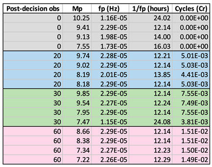
The single-sided spectrum of the post-filtered 6-hour windowed pre-decision means revealed that pre-decision means had peak magnitudes that differed depending on the post-decision duration (Table 1, second column). This result echoed the initial qualitative observation that the periodicities of pre-decision photon count means seemed to be related to post-decision durations, and better quantified the CADS hypothesis by showing that the peak magnitudes of pre-decision means specific to different post-decision durations can be estimated from peak frequencies and the post-decision durations themselves.
Specifically, the best estimation of magnitudes at the first four frequency peaks required considering the frequency at the peak magnitude (fp) and the duration of the post-decision observation period to obtain the unitless cycles per run (Cr):
obsp = post-decision obs * 11 s
Cr = fp*obsp.
To get an intuitive feel for the meaning of cycles per run in this context requires thinking of the period at the peak frequency as a window tuned to observations of runs of a given post-decision duration, with cycles per run indicating the number of possible post-decision durations that could fit in that window. Plotting Cr against the empirically obtained peak magnitudes of the pre-decision count means (Figure 8A) further shed light on the relationship between cycles per run and peak magnitudes (Mp). The best fit was a linear equation with R2=.982:
Mp = -80.056 * Cr + 9.147.
This equation, derived from mean peak frequencies, also fit the individual data values almost as well as the best fit equation (Figure 8B), suggesting the originating data were not inconsistent with the mean-derived best fit. In addition, as would be expected, the best fit for the mean of the four top peaks (3) was very close to the best fit for the largest peak magnitudes alone (R2=.961; data not shown):
where Mp1 indicates the largest peak magnitude and Cr1 indicates the cycles per run at the corresponding peak frequency. Equations (3) and (4) are two versions of the CADS equation that may be useful in different circumstances.
Mp1 = -78.753 * Cr1 + 9.1612,
Because the goodness of fit to the data was impressive, the originating data were examined more closely to determine whether the mean pre-decision counts somehow reflected the post-decision observation durations in a previously unappreciated way. For instance, it might have been possible that the four post-decision duration datasets contained a different number of runs, and in some way the number of runs affected the pre-decision means in the 6-hour windows. However, the number of post-decision durations selected in each of these four datasets was approximately 10.3 across post-decision durations, with a range of 10.2 to 10.32 and there were no significant differences in the number of post-decision durations across different post-decision duration datasets. In addition, the number of post-decision durations across the 1459 6-hour windows was not significantly correlated with pre-decision means in the same 6-hour windows for any post-decision duration (highest R2=.0009, p>.230). Finally, the independent frequency analyses for each of the four post-decision duration datasets used the same sampling rate (6 hours) and the same frequency axes for the resulting spectra were obtained. Thus, there was no information about post-decision durations embedded in the four independent time series of pre-decision means, suggesting that the CADS equation truly characterizes a relationship between pre-decision photon counts and the post-decision observation duration in CADS experiments.
4. Discussion
This replication attempt was successful in that it allowed further characterization of the periodicities qualitatively observed in the initial CADS experiments [14,15] and provided a quantitative description of the observed relationship between pre-decision photon count means and post-decision observation durations. In addition, independent of the CADS effect, an apparently novel relationship between photon counts and lunar phase was documented. The lunar phase effect was found serendipitously in the pre-decision means, but based on the time series data for the entire year-long experiment (Figure 2A), it is likely that this effect is not limited to pre-decision means. Correlation does not imply causation, but because photons on earth in an enclosed optical box are unlikely to affect phases of the moon, the strong implication from this result is that lunar phase affects photons via a mechanism that remains to be understood. One obvious possibility is the effect is obtained through changes in moon luminance, but the dataset shows troughs during both the new and full moons, and these provide very different luminance levels. Other possibilities are either gravitational [19] or magnetospheric [20] influences that vary with the lunar cycle and therefore very slightly influence spacetime curvature or electromagnetic fields (respectively) on earth. The importance of lunar phase impacts on individual photon absorption and/or emission rates may only be appreciated by engineers and scientists working with single particle or low-light systems, but this finding could reasonably influence the metrology/precision timing as well as quantum computation fields.
Beyond the lunar effect, a more precise CADS hypothesis emerged from examining the time series and frequency spectra of pre-decision means recorded before the decision about post-decision duration was made. This effect was obtained with post-decision durations in the seconds-to-minutes range, and was demonstrated by examining pre-decision means in 6-hour windows. The effect did not seem to be confounded by classical informational leakage about the post-decision duration, such as a potential (but not actualized) relationship with the number of runs of each post-decision duration. The two versions of the CADS equation (3) and (4) allowed the estimation of empirically derived values – the magnitudes at the peak frequencies of pre-decision means – for each of the four post-decision durations. This estimation was based on a combination of the experimentally controlled post-decision durations and the empirically derived peak frequencies of the single-sided spectrum of pre-decision photon count means. Thus the CADS equation cannot be used to predict empirical results prior to the first time an experiment with given post-decision durations is performed, but it could be used to determine unknown post-decision durations once peak frequencies and magnitudes are known.
Overall, the results suggest that the post-decision duration of a single experimental run in a CADS experiment is entangled with the pre-decision photon counts in a way that can be observed in spacetime via a reliable periodicity apparent at the group-run level (Figure 7 and Figure 8). It is also possible that the same entanglement could be observed during the experiment at the single-run level, but this strong version of the CADS hypothesis remains to be tested. However, given that the sigmas obtained with an average of 10 runs were often at ceiling (example: Figure 6B), it is not really the single-run reliability of the effect that is in question here, instead it is the question of whether a message can be sent to the past using the CADS methodology [21].
Taken in the context of the existing literature, this replication and characterization of the CADS effect may provide evidence for interpretations of quantum mechanics that admit all-at-once, acausal, or retrocausal calculations of events in the present, such as many-worlds [22,23], transactional [24,25], and two-state vector formalism [26,27] interpretations of quantum mechanics. However, one key difference between the CADS effect and other effects that support these interpretations is that with the CADS effect, there is no need for inferring what happened in the past and explaining how a measured effect in the future influenced the past or the branching of worlds on a given run of the experiment. While most retrocausality experiments use the “prepare-transform-measure” or “prepare-choose-measure” sequence [28], the CADS effect is obtained by a “prepare-measure-choose-measure” sequence. Photons are absorbed and counts are observed by the computer prior to the choice about the future duration. Thus branching occurs, the handshake is complete, or the waveform is collapsed (depending on your model), before the future is selected. For this reason, the fit with the many-worlds, transactional interpretation, and two-state vector formalism interpretations may be poor, because it seems one has to propose that the history of these already-observed counts is changed in an observer’s already-recorded spacetime, according to the eventual post-decision observation durations.
The CADS effect seems to support an ”all-at-once” calculation of events in spacetime [28]. The author’s speculation is that groups of photons are entangled across time by classical shared-group boundary conditions (i.e., on-off times) are differentiated from each other in some kind of informational structure preceding emergence into spacetime. The emergence of this structure is perceived by us as a dynamic spacetime evolution. In this picture, duration would be a fundamental feature of any object like spin or mass. However, because dynamic models of the universe have dominated until recently [16] and the focus has been on objects rather than events, duration has been ignored as a fundamental feature. The universe must distinguish differences in fundamental features so that there can be different things. For instance, there must be a way to distinguish 9 from 10 grams when mass of an event is measured. According to this line of thinking, the CADS effect may be a way to glimpse this fundamental feature for multiple-particle events with measurements that occur across the seconds-to-minutes time scale. More poetically, each event of a different duration has its own distinct signature woven through the universal calculation of spacetime.
Follow-up CADS experimentation using real-time single-run estimation of future post-decision observation durations will be required to determine whether a message can be sent backwards in time using CADS, to shed greater light on the quantum characteristics of the CADS effect, and to determine which interpretations of quantum mechanics are consistent with this robust and surprising effect. Even before these experiments are completed, applications of the group-run based CADS effect ought to be considered by designers of photonics quantum computing systems.
Funding
This research received no external funding.
Data Availability Statement
The original pre- and post-filtered time series data will be available at Figshare once the paper is published in Entropy and are available to reviewers during the review process here: https://tinyurl.com/CADS2025.
Acknowledgments
The author is grateful to Dr. Winthrop Williams of the UC Berkeley Advanced Physics Laboratory for creating this long-time-frame replication of the original CADS effect using his own materials, design, and equipment – and for providing the data from that experiment for further analysis here, as well as suggested analysis Matlab scripts that were modified and extended by the author for these analyses. The author is also grateful to software engineer Carl Evaristo at KVK who also built his own shorter replication, using his own materials, and provided the data from that experiment for further analysis that helped confirm some of the results shown here (data not shown). Additionally, the author would like to thank Daniel Sheehan at University of San Diego, Dick Shoup, and Sir Roger Penrose for supportive and insightful discussions about this work.
Conflicts of Interest
The author declares no conflicts of interest.
Abbreviations
The following abbreviations are used in this manuscript:
| ANOVA | Analysis of variance |
| CADS | Causally ambiguous duration sorting |
| CMOS | Complementary metal oxide semiconductor |
| DD | Two digits for day |
| FFT | Fast Fourier transform |
| FPGA | Field programmable gate array |
| Hz | Hertz |
| IC | Integrated circuit |
| LED | Light-emitting diode |
| MM | Two digits for month |
| nm | Nanometers |
| Obs | Observations |
| RC | Resistor-capacitor |
| s | Second(s) |
| SEM | Standard error of the mean |
| YYYY | Four digits for year |
References
- Aharonov, Y.; Popescu, S.; Tollaksen, J. A time-symmetric formulation of quantum mechanics. Physics Today 2010, 63, 27–32. [Google Scholar] [CrossRef]
- Cohen, E.; Cortês, M.; Elitzur, A.; Smolin, L. Realism and causality. I. Pilot wave and retrocausal models as possible facilitators. Physical Review D 2020, 102, 124027. [Google Scholar] [CrossRef]
- Cohen, E.; Cortês, M.; Elitzur, A.C.; Smolin, L. Realism and causality. II. Retrocausality in energetic causal sets. Physical Review D 2020, 102, 124028. [Google Scholar] [CrossRef]
- Cramer, J.G. The arrow of electromagnetic time and the generalized absorber theory. Foundations of Physics 1983, 13, 887–902. [Google Scholar] [CrossRef]
- Leifer, M.S.; Pusey, M.F. Is a time symmetric interpretation of quantum theory possible without retrocausality? Proceedings of the Royal Society A: Mathematical, Physical and Engineering Science 2017, 473, 20160607. [Google Scholar] [CrossRef]
- Price, H. Does time-symmetry imply retrocausality? How the quantum world says “Maybe”? Studies in History and Philosophy of Science Part B: Studies in History and Philosophy of Modern Physics 2012, 43, 75–83. [Google Scholar] [CrossRef]
- Shimony, A. Conceptual foundations of quantum mechanics. In The New Physics; Davies, P., Ed.; Cambridge University Press: Cambridge, UK, 1989; pp. 373–395. [Google Scholar]
- Wharton, K. A new class of retrocausal models. Entropy 2018, 20, 410. [Google Scholar] [CrossRef]
- Song, X.; Salvati, F.; Gaikwad, C.; Yunger Halpern, N.; Arvidsson-Shukur, D.R.; Murch, K. Agnostic phase estimation. Physical Review Letters 2024, 132, 260801. [Google Scholar] [CrossRef] [PubMed]
- Arvidsson-Shukur, D.R.; McConnell, A.G.; Yunger Halpern, N. Nonclassical advantage in metrology established via quantum simulations of hypothetical closed timelike curves. Physical Review Letters 2023, 131, 150202. [Google Scholar] [CrossRef] [PubMed]
- Castagnoli, G. Highlighting the mechanism of the quantum speedup by time-symmetric and relational quantum mechanics. Foundations of Physics 2016, 46, 360–381. [Google Scholar] [CrossRef]
- Castagnoli, G. Unobservable causal loops as a way to explain both the quantum computational speedup and quantum nonlocality. Physical Review A 2021, 104, 032203. [Google Scholar] [CrossRef]
- Rieffel, E.; Polak, W. An introduction to quantum computing for non-physicists. ACM Computing Surveys (CSUR) 2000, 32, 300–335. [Google Scholar] [CrossRef]
- Mossbridge, J.A. The influence of future durations on past photon counts in an optical system. In Proceedings of the 2019 Annual Meeting of the APS Far West Section, Stanford, USA, 02 November 2019. Available online: https://figshare.com/articles/figure/Future_Photon_Figure_1_pdf/9964976 (accessed on 10 January 2025).
- Mossbridge, J.A. Long time-frame causally ambiguous behavior demonstrated in an optical system. ResearchGate white paper 2021. Available online: https://www.researchgate.net/publication/349106030_Long_time-frame_causally_ambiguous_behavior_demonstrated_in_an_optical_system (accessed on 10 January 2025).
- Silberstein, M.; Stuckey, W.M.; McDevitt, T. Beyond the Dynamical Universe: Unifying Block Universe Physics and Time as Experienced; Oxford University Press: Oxford, UK, 2018. [Google Scholar]
- Williams, W.T.; Mossbridge, J.A. Replication study of causally ambiguous duration sorting (CADS). In Proceedings of The Journal of Parapsychology, Online conference, 29 July 2022. Available online: https://www.youtube.com/watch?v=Yh7mVGtorNM (accessed on 10 January 2025).
- Minkukel Plus. Available online: https://en.minkukel.com/various/calculating-moon-phase/ (accessed on 10 January 2025).
- Goodkind, J.M. The superconducting gravimeter. Review of scientific instruments 1999, 70, 4131–4152. [Google Scholar] [CrossRef]
- Kivelson, M.G. Moon–magnetosphere interactions: A tutorial. Advances in Space Research 2004, 33, 2061–2077. [Google Scholar] [CrossRef]
- Shoup, R. Understanding retrocausality—Can a message be sent to the past? In Proceedings of the AIP Conference Proceedings, San Diego, USA, 29 Nov 2011, 255-278. Available online: https://pubs.aip.org/aip/acp/article-abstract/1408/1/255/719116/Understanding-Retrocausality-Can-a-Message-Be-Sent?redirectedFrom=PDF (accessed on 10 January 2025).
- Dewitt, B.S.; Graham, N. (Eds.) The Many-Worlds Interpretation of Quantum Mechanics: A Fundamental Exposition by Hugh Everett, III, with Papers by JA Wheeler, BS DeWitt, LN Cooper and D. Van Vechten, and N. Graham; Princeton University Press: Princeton, USA, 1973. [Google Scholar]
- Everett III, H. "Relative state" formulation of quantum mechanics. Reviews of modern physics 1957, 29, 454–462. [Google Scholar] [CrossRef]
- Cramer, J.G. The Transactional Interpretation of Quantum Mechanics. Reviews of Modern Physics 1986, 58, 647–687. [Google Scholar] [CrossRef]
- Kastner, R.E. The transactional interpretation of quantum mechanics: A relativistic treatment; Cambridge University Press: Cambridge, UK, 2022. [Google Scholar]
- Aharonov, Y.; Bergmann, P.G.; Lebowitz, J.L. Time symmetry in the quantum process of measurement. Physical Review 1964, 134, B1410–B1416. [Google Scholar] [CrossRef]
- Aharonov, Y.; Vaidman, L. Complete description of a quantum system at a given time. Journal of Physics A: Mathematical and General 1991, 24, 2315–2328. [Google Scholar] [CrossRef]
- Adlam, E. Two roads to retrocausality. Synthese 2022, 200, 422. [Google Scholar] [CrossRef]
Figure 1.
Protocol schematic showing all four equiprobable post-decision durations following the pre-decision period. Not shown: 6 s warm-up period preceding the pre-decision observations, and 3.2 s additional time for each run (empirically derived).
Figure 1.
Protocol schematic showing all four equiprobable post-decision durations following the pre-decision period. Not shown: 6 s warm-up period preceding the pre-decision observations, and 3.2 s additional time for each run (empirically derived).
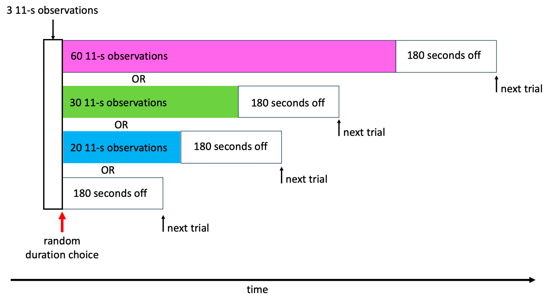
Figure 2.
Time series graphs of photon counts in 11-s observation windows across 365 days. Left: pre-filtered, original raw signal. Right: high-pass filtered signal.
Figure 2.
Time series graphs of photon counts in 11-s observation windows across 365 days. Left: pre-filtered, original raw signal. Right: high-pass filtered signal.
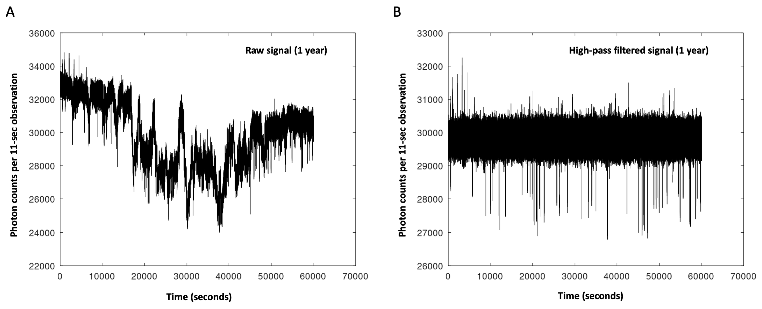
Figure 3.
FFT of year-long signal after high-pass filtering. Red asterisk indicates the 6-hour period range, which was used for the periodicity analysis.
Figure 3.
FFT of year-long signal after high-pass filtering. Red asterisk indicates the 6-hour period range, which was used for the periodicity analysis.
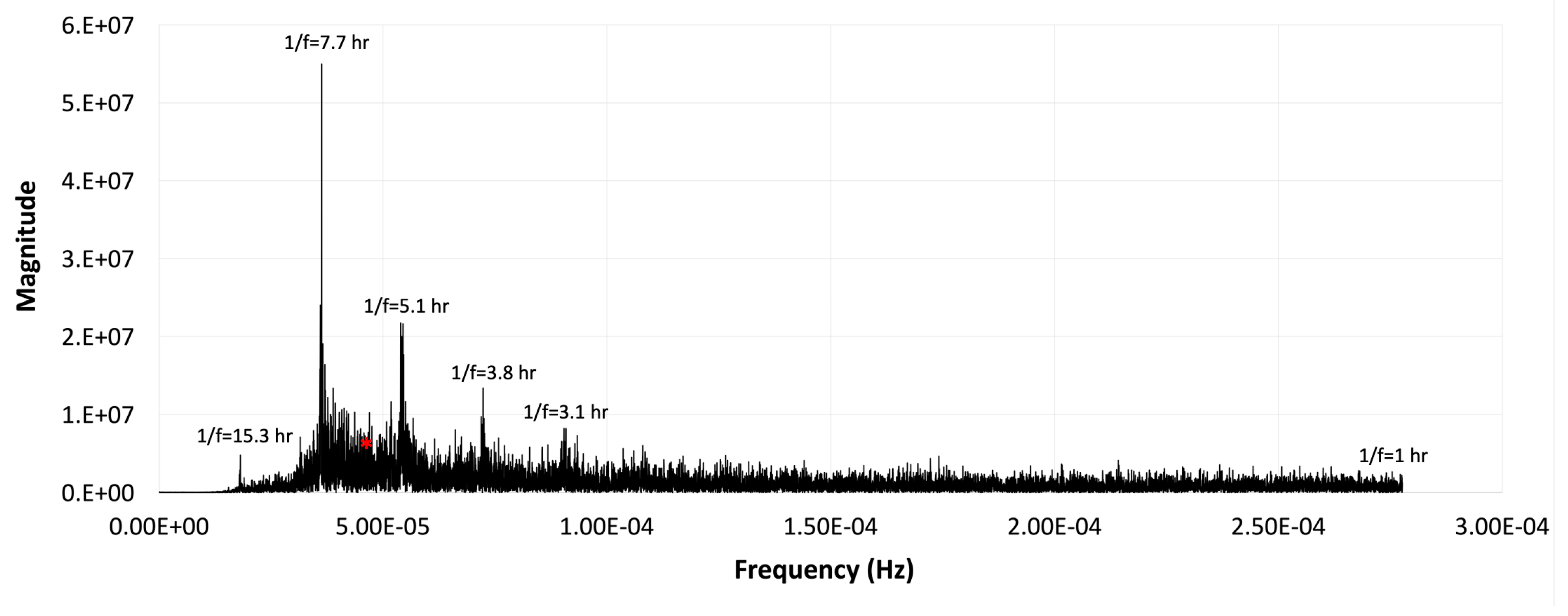
Figure 4.
Mean pre-decision photon counts from pre-filtered time series data plotted against the lunar phase for the time at which the absorptions were recorded. Error bars give +/- 1 standard error of the mean (SEM).
Figure 4.
Mean pre-decision photon counts from pre-filtered time series data plotted against the lunar phase for the time at which the absorptions were recorded. Error bars give +/- 1 standard error of the mean (SEM).
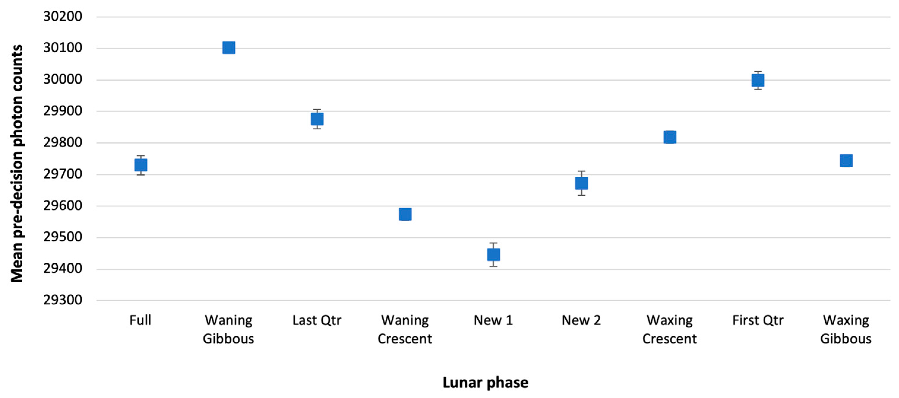
Figure 5.
Mean pre-decision photon counts from post-filtered data plotted against the number of post-decision observations following the duration decision. Error bars give +/- 1 SEM.
Figure 5.
Mean pre-decision photon counts from post-filtered data plotted against the number of post-decision observations following the duration decision. Error bars give +/- 1 SEM.
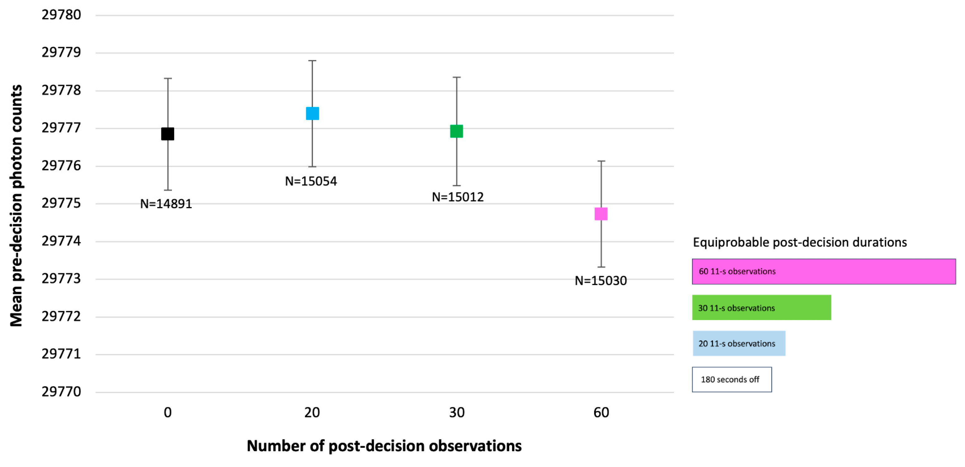
Figure 6.
Blue dots represent t-scores (top) and resulting conservative Sigmas (bottom) in comparisons between 6-hour windowed pre-decision means for 60 vs. 20 post-duration decision observations. Lines off the top graph indicate t-scores smaller or larger than 40. The artificial ceiling on sigma defines the top line of the bottom graph. Dates on x-axes are in the YYYY-MM-DD convention.
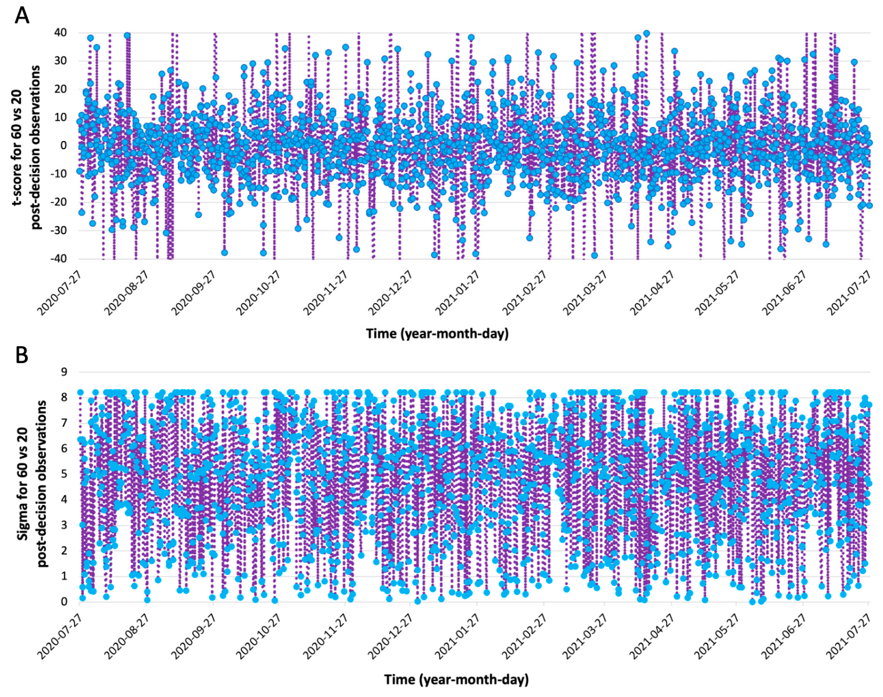
Figure 7.
Mean of conservative sigmas from 6-hour windows for each comparison of pre-decision means between post-decision durations for pre-filtered (blue) and post-filtered (black) data.
Figure 7.
Mean of conservative sigmas from 6-hour windows for each comparison of pre-decision means between post-decision durations for pre-filtered (blue) and post-filtered (black) data.
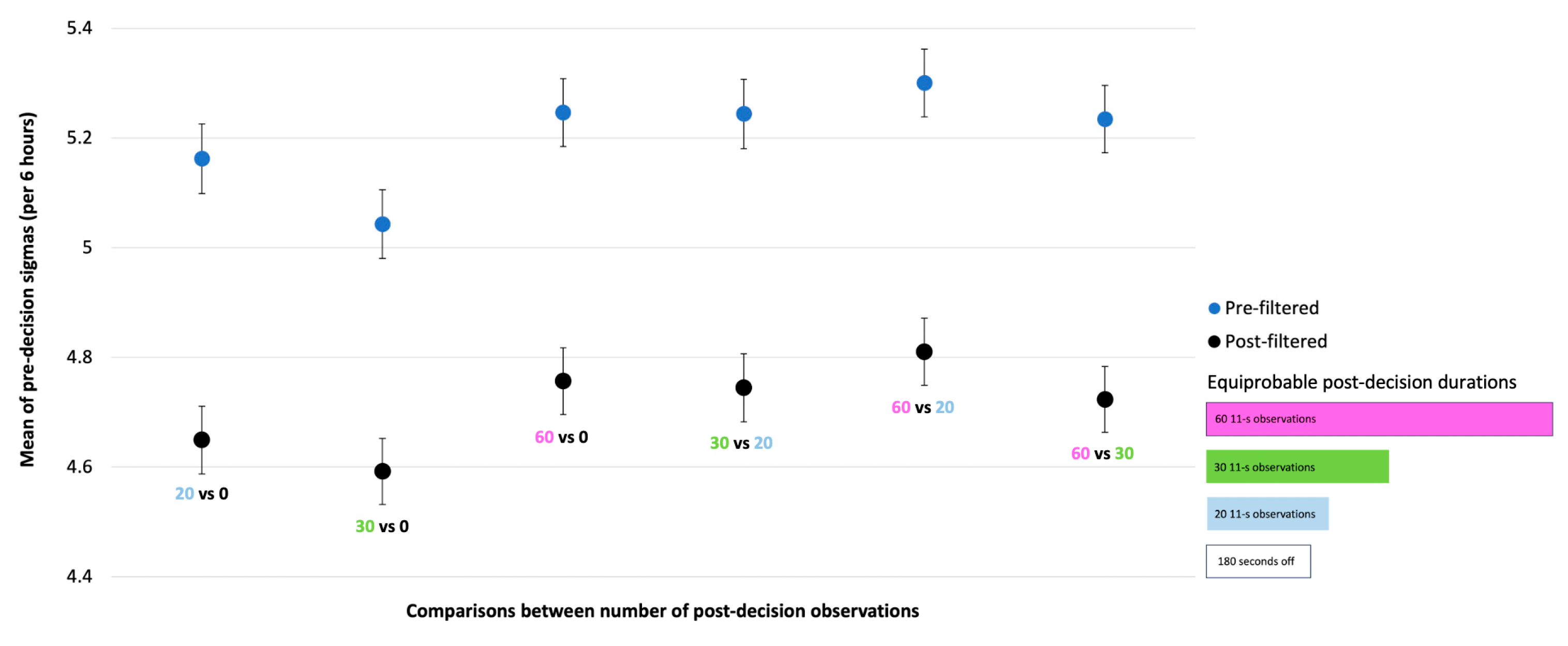
Figure 8.
A: Mean magnitudes (Mp) vs. mean cycles per run (Cr) across the top four peaks of the pre-decision mean frequency-analyzed data. B: Same as A except for each of the top four peaks.
Figure 8.
A: Mean magnitudes (Mp) vs. mean cycles per run (Cr) across the top four peaks of the pre-decision mean frequency-analyzed data. B: Same as A except for each of the top four peaks.
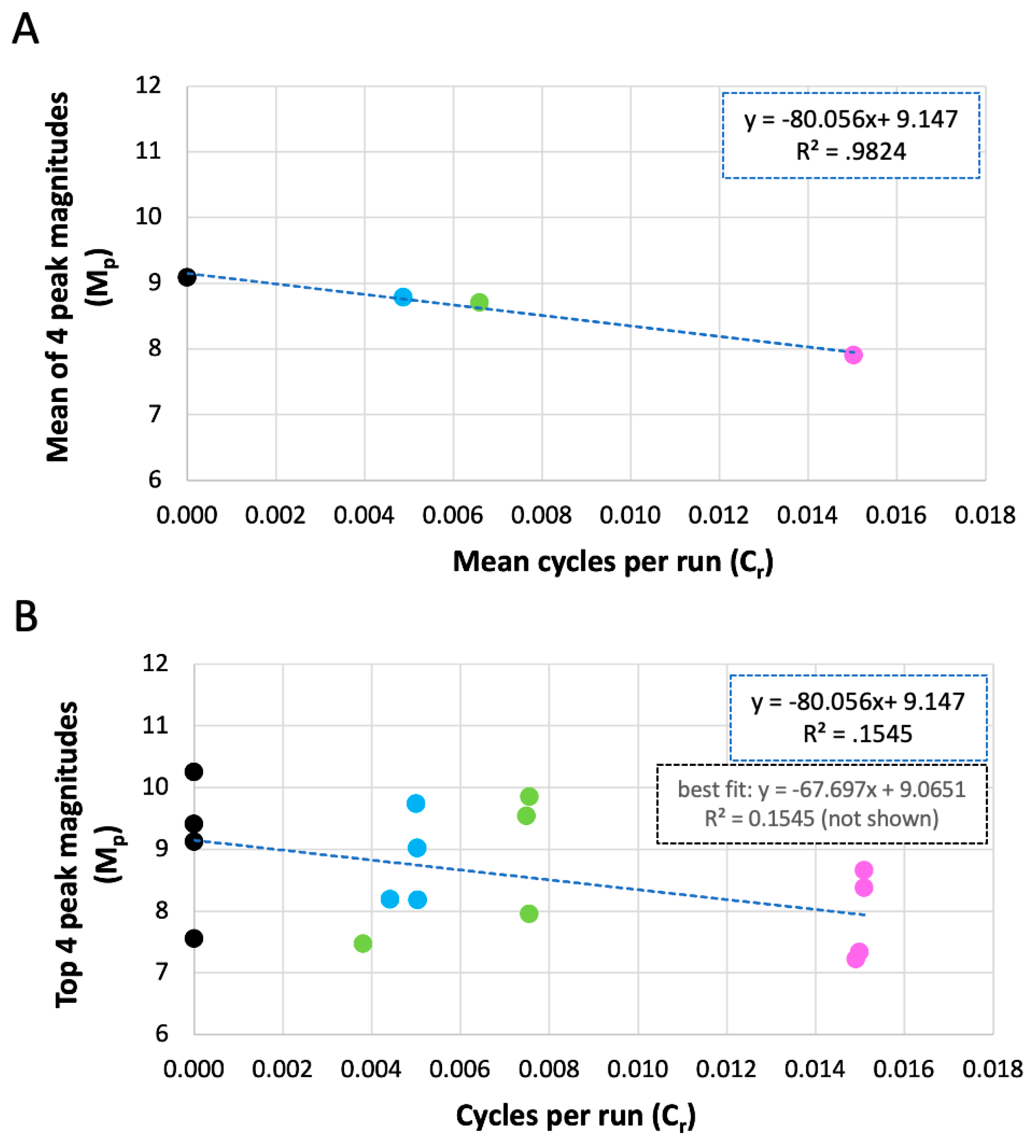

Table 1.
Top four magnitudes (Mp), second column, listed for each each post-decision observation duration (first column) with frequencies at those peak magnitudes (fp), periods in hours (1/fp), total and cycles per run (Cr) for the frequency-analyzed 6-hour windowed post-filtered pre-decision mean data.
 |
Disclaimer/Publisher’s Note: The statements, opinions and data contained in all publications are solely those of the individual author(s) and contributor(s) and not of MDPI and/or the editor(s). MDPI and/or the editor(s) disclaim responsibility for any injury to people or property resulting from any ideas, methods, instructions or products referred to in the content. |
© 2025 by the authors. Licensee MDPI, Basel, Switzerland. This article is an open access article distributed under the terms and conditions of the Creative Commons Attribution (CC BY) license (http://creativecommons.org/licenses/by/4.0/).
Copyright: This open access article is published under a Creative Commons CC BY 4.0 license, which permit the free download, distribution, and reuse, provided that the author and preprint are cited in any reuse.


