
Submitted:
09 March 2025
Posted:
10 March 2025
You are already at the latest version
Abstract
In major seismic events (e.g., the 2011 Tohoku-Taiheiyou-Oki Earthquake, the 2016 Kumamoto Earthquake in Japan, and the 2023 Kaharamanmaraş Earthquake in Turkey), many building structures are subjected to a series of earthquake sequences. Therefore, evaluating the seismic demands of building structures under earthquake sequences is important. This article proposes extended critical pseudo-multi impulse (PMI) analysis considering sequential input. In this extended PMI analysis, seismic input is modeled as two parts of multi impulses (MIs). The parameters of the seismic input are (a) the pulse velocities of the first and second MIs, (b) the number of impulsive lateral forces of the first and second MIs, and (c) the length of the interval between the two MIs. In the numerical analysis, the peak and cumulative responses of an eight-story reinforced concrete (RC) moment-resisting frame (MRF) with steel damper columns (SDCs) subjected to the earthquake sequence recorded during the 2016 Kumamoto Earthquake were predicted using the proposed extended critical PMI analysis. For this prediction, the pulse velocities of the first and second MIs were determined based on the maximum momentary input energy of the input ground motions. The main findings are as follows. (1) The accuracy of the predicted peak response of RC MRFs with SDCs subjected to earthquake sequences from the extended critical PMI analysis was satisfactory. (2) The accuracy of the cumulative response of RC MRFs with SDCs depended on the ground motion records and the number of impulsive lateral forces of the first and second MIs.
Keywords:
reinforced concrete moment-resisting frame
; steel damper column
; earthquake sequences
; incremental critical pseudo-multi impulse analysis
; maximum momentary input energy
; peak displacement
; cumulative energy
1. Introduction
1.1. Background and Motivations
The purpose of seismic design of structures is to provide enough seismic capacity to withstand expected large earthquakes. Although structures have been subjected to series of earthquake sequences in past major seismic events (e.g., the 2011 Tohoku-Taiheiyou-Oki Earthquake in Japan, the 2016 Kumamoto Earthquake in Japan, and the 2023 Kaharamanmaraş Earthquake in Turkey), the “design” earthquake considered in most seismic design codes is a single seismic event. In most modern seismic design codes, a structure designed in a ductile manner (e.g., a moment-resisting frame; MRF) is allowed to respond beyond the elastic range in the case of large earthquakes. When the “design” earthquake occurs, some level of plastic deformation of structural members in such MRFs is expected. However, in the case of an earthquake sequence, the accumulation of damage (seismic energy absorption) in structural members may be progressive. Therefore, the influence of earthquake sequences on the seismic performance of building structures should be considered for better seismic design.
The steel damper column (SDC; Katayama et al., 2000) is an energy dissipation device that is suitable for mid- and high-rise reinforced concrete (RC) housing buildings. SDCs can be easily installed in a RC MRF because they minimize obstacles in architectural planning. An RC MRF with SDCs can be considered as a damage-tolerant structure (Wada et al., 2000); SDCs behave as sacrificial members that absorb seismic energy prior to the RC beams and columns. Such structures are expected to perform better during earthquake sequences than an RC MRF without energy dissipation devices. The author’s research group has studied a simplified seismic design procedure for an RC MRF with SDCs (Mukouyama et al., 2021), and a simplified procedure to predict the peak and cumulative responses of an RC MRF with SDCs based on the energy concept (Fujii and Shioda, 2023). In the case of earthquake sequences, the nonlinear responses of a ten-story RC MRF with and without SDCs under the records of the 2016 Kumamoto Earthquake were examined based on NTHA results in a previous study (Fujii, 2022). Extension of the simplified procedure (Fujii and Shioda, 2023) for application in the case of an earthquake sequence is the next target of study. To this end, the change of characteristics of a structure due to the response the structure previously experienced (e.g., the elongation of natural periods or reduction of seismic absorption capacity) must be considered. Many researchers have investigated the responses of structures under earthquake sequences by conducting NTHA. Most of these studies can be divided into two groups according to the ground motion sequences: as-recorded ground motion sequences, and “artificial” ground motion sequences (e.g., applying the same ground acceleration several times (repeated approach), or choosing different ground accelerations at random (randomized approach)).
Mahin (1980) studied the response of a single-degree-of-freedom (SDOF) model with an elastic-perfectly-plastic hysteresis model subjected to the mainshock of 1972 Managua Earthquake with two large aftershocks. Amadio et al. (2003) studied the nonlinear response of SDOF systems subjected to repeated earthquakes, applying a repeated approach. Similarly, Hatzigeorgiou and Beskos (2009) studied the inelastic displacement ratio for SDOF systems by applying the repeated approach. One reason to apply the repeated approach is that the study will be very complex when real seismic sequential accelerations with different characteristics (e.g., frequency, duration) are applied. To avoid bias caused by the repeated approach, Hatzigeorgiou (2010a; 2010b) analyzed the nonlinear response of SDOF systems subjected to random sequences. In addition, Hatzigeorgiou and Liolios (2010) studied the nonlinear response of a multi-degree-of-freedom (MDOF) system subjected to as-recorded ground motion sequences, analyzing the response of planar RC frames. Ruiz-García and Negrete-Manriquez (2011) compared the nonlinear response of planar steel frames subjected to as-recorded ground motion sequences and artificial ground motion sequences. They concluded that the artificial sequences (repeated approach) led to overestimation of the maximum lateral demands. They also pointed out that the repeated approach was insufficient to model the earthquake sequences, because the frequency characteristics of the aftershock records differed from those of corresponding mainshock records. The nonlinear response of frame models subjected to artificial sequential earthquakes (repeated approach or random approach) were compared by Ruiz-García (2012a).
Since 2012, the number of studies on the nonlinear responses of structures subjected to earthquake sequences has been increasing. One reason for this may be the occurrences of the Christchurch Earthquake in New Zealand in 2010–2011 and the 2011 Tohoku–Taiheiyo–Oki Earthquake in Japan. As-recorded earthquake sequences have been used in many studies after 2010 (Abdelnaby and Elnashai, 2014; Abdelnaby, 2016; Di Sarno, 2013; Di Sarno and Amiri, 2019; Di Sarno and Pugliese, 2021; Di Sarno and Wu, 2021; Elenas et al., 2017; Hatzivassiliou and Hatzigeorgiou, 2015; Hosseinpour and Abdelnaby, 2017; Hoveidae and Radpour, 2021; Kagermanov and Gee, 2019, Oyguc et al., 2018; Qiao et al., 2020; Ruiz-García, 2012b; Ruiz-García, 2013; Ruiz-García et al., 2018; Ruiz-García and Olvera, 2021; Soureshjani and Massumi, 2022; Yaghmaei-Sabegh and Ruiz-García, 2016; Yaghmaei-Sabegh and Mahdipour-Moghanni, 2019; Wen et al., 2020; Zhai et al., 2012; Zhai et al., 2014). In addition, artificial ground motion sequences have been applied in many studies since 2012 (Abdelnaby and Elnashai, 2015; Faisal et al., 2013; Goda, 2012a; Goda, 2012b; Goda, 2014; Gota et al., 2015; Han et al., 2017; Orlacchio et al., 2021; Oyguc et al., 2023; Ruiz-García et al., 2012; Ruiz-García et al., 2013; Tesfamariam et al., 2015; Tesfamariam and Goda, 2017; Yang et al., 2016; Yang et al., 2019; Zhai et al., 2013). Specifically, Yaghmaei-Sabegh and Ruiz-García (2016) studied the case of a “doublet earthquake,” a pair of seismic events that take place closely spaced in time and location; this differs from the mainshock–aftershock sequences on which most studies have focused. They also showed that in a doublet earthquake, the characteristics of the first and second mainshock differ. Therefore, even in the case of a doublet earthquake, the repeated approach is unrealistic. To verify the artificial sequence method, Gota (2012b) compared the probability of peak ductility demand calculated from an artificial sequence and an as-recorded sequence. In this generation method of artificial mainshock–aftershock sequences, the generalized Ohmori’s law was implemented. The calculated ductility demand from Gota’s artificial sequence was consistent with that calculated using as-recorded sequences. A similar conclusion was reached by Yaghmaei-Sabegh and Mahdipour-Moghanni (2019).
The brief review of these studies above indicates that the kinds of sequential input considered for analyzing the behavior of structures is key. As described above, the repeated approach, although simple, is unrealistic. The use of as-recorded sequences is the most realistic; however, because the characteristics of aftershock ground motions are different from those of mainshock ground motions, the complexity of the analysis results would increase.
The term “energy” is useful for understanding the nonlinear behavior of structures (e.g., Akiyama, 1985; 1999, Uang and Bertero, 1990). The total input energy, or the equivalent velocity of the total input energy (), is an important seismic intensity parameter
related to the cumulative response (Akiyama, 1985; 1999). In addition, the
maximum momentary input energy, or the equivalent velocity of the maximum
momentary input energy (), is an important seismic intensity parameter related to the peak response (Hori and Inoue, 2002). Because the damage accumulated in the structure is critical in cases of earthquake sequences, it is reasonable to discuss the response under earthquake sequences in terms of energy. Zhai et al. (2016) analyzed the inelastic input energy spectra for mainshock–aftershock sequences. Gentile and Galasso (2021) proposed hysteresis energy-based state-dependent fragility for ground motion sequences. Following that study, Pedone et al. (2023) proposed an energy-based procedure for seismic fragility analysis of mainshock-damaged buildings. More recently, Alıcı and Sucuoğlu (2024) analyzed the inelastic input energy spectra of the recorded mainshock–aftershock sequences of the February 6, 2024, Kahramanmaraş earthquakes. Donaire-Ávila et al. (2024) analyzed the cumulative dissipated energy of RC building models under earthquake sequences.
Kojima and Takewaki (2015a; 2015b; 2015c) introduced the concepts of the critical double impulse (DI) and critical multi impulse (MI) as substitutes for near-fault and long-duration earthquake ground motions, respectively. These concepts simplify seismic input by considering the most severe case for the structure of interest. In these studies, the critical response of an undamped SDOF model with elasto-plastic behavior was analyzed in the simple equations considering the energy balance (Kojima and Takewaki, 2015a; Kojima and Takewaki, 2015b; Kojima and Takewaki, 2015c). Then, Akehashi and Takewaki introduced the pseudo-double impulse (PDI) (Akehashi and Takewaki 2021), and pseudo-multi impulse (PMI) (Akehashi and Takewaki 2022a) to form the MDOF model. In PDI and PMI analysis, the MDOF model oscillated predominantly in a single mode, considering the impulsive lateral force corresponding to a certain mode vector. When the impulsive lateral force corresponding to the first mode vector was considered, the MDOF model oscillated predominantly in the first mode. In addition, Akehashi and Takewaki (2022b) proposed an adjustment method of DI to work as a real earthquake. Following their studies, this author has applied their PDI and PMI analyses to RC MRF with SDCs (Fujii, 2024a; 2024b), to verify the simplified procedure to predict the peak and cumulative responses of an RC MRF with SDCs based on the energy concept (Fujii and Shioda, 2023).
To the author’s knowledge, NTHA is thus far the only method to analyze the response of structures subjected to earthquake sequences. However, the results obtained from NTHA are too complex to derive general conclusions. This is because NTHA results are intricately intertwined with nonlinear structural characteristics and ground motion characteristics. In the case of an earthquake sequence, the complexity increases because of the combined mainshock–aftershock (or foreshock–mainshock, or doublet earthquake) ground motions. Therefore, extension of critical PMI analysis for the case of earthquake sequences may be a promising alternative. This is because the results of critical PMI analysis make it much easier to understand nonlinear structural characteristics. This was the main motivation of this study.
1.2. Objectives
In this article, extended critical PMI analysis considering sequential input is proposed. The peak and cumulative responses of an eight-story RC MRF with SDCs subjected to the earthquake sequence recorded in the 2016 Kumamoto Earthquake were predicted using extended critical PMI analysis. This analysis is the updated version of the analysis reported in previous studies (Fujii 2024a and 2024b). In this proposed analysis, the seismic input was modeled as two parts of MIs. The parameters of the seismic input were (i) the pulse velocities of the first and second MI, (ii) the number of impulsive lateral forces of the first and second MI, and (iii) the length of the interval between the two MIs. For better prediction of structural responses under earthquake sequences, this study addresses the following questions.
- (I)
- How should the pulse velocities of the first and second MIs be determined for better prediction of the peak response? Can they be determined based on the maximum momentary input energy spectrum (VΔE spectrum) of the input ground motions?
- (II)
- How can the number of impulsive lateral forces of the first and second MIs be determined for better prediction of the cumulative response (e.g., the cumulative strain energy of a damper panel in SDC)?
- (III)
- Di Sarno et al. (2020) and Amiri et al. (2021) pointed out the importance of considering the relative difference between the incident angles of the mainshock and subsequent aftershocks. Although a planar frame analysis is considered here, the signs of the two MIs, which correspond to the conventional aftershock polarity (positive or negative), must still be accounted for. How will the signs of two MIs affect the responses of structures?
In the study of Akehashi and Takewaki (2022b), the intensity of pulses was determined based on the cumulative input energy spectrum ( spectrum). They showed that the total input energy
and cumulative strain energy obtained from DI analysis agreed well with the
results obtained from NTHA using ground motion records, whereas the peak drift
obtained from DI analysis was much larger than that obtained from NTHA using
ground motion records. However, the pulse velocity of the MIs was determined
based on the maximum momentary input energy spectrum ( spectrum) in this study because of the following reasons. Several researchers have carried out the experimental study conducting the low-cycle fatigue of RC members (e.g., El-bahy et al., 1999; Xing et al. 2017; Marder 2018). Specifically, El-bahy et al. (1999) showed from the test results of circular RC bridge columns that the specimen which had been cycled 150 times at a lateral drift of 2 % showed virtually no sign of damage or deterioration, while the specimen which had been cycled at a lateral drift of 5.5 % failed less than 10 cycles. Similarly, Xing et al. (2017) showed from the test results of rectangular RC ductile columns that the specimen which had been cycled at a ductility ratio 2 (lateral drift of 2.6 %) failed after 268 cycles, while the specimen which had been cycled 1000 times at a ductility ratio 1 (lateral drift of 1.3 %) failed after 136 cycles at a ductility ratio 2. Following their studies, Elwood et al. (2021) concluded that, in case of ductile RC MRFs, “cyclic loading up to 2% drift had a limited impact on the deformation capacity of column specimens with up to 0.1 axial load ratio.” When conducting the seismic design of an RC MRF with SDCs, the peak story drift would be set less than 2% for the design earthquake. Therefore, for the analysis of an RC MRF with SDCs in this study, the pulse velocity was adjusted based on the spectrum for predicting the peak response accurately.
Note that Miyake (2006) compared the low-fatigue test results of H-shaped steel columns and RC columns. In his study, he obtained (hysteretic dissipated energy) – (displacement amplitude) relationship of those members, by combining the (displacement amplitude) – (cycles to failure) relationship and (hysteretic dissipated energy) – (cycles to failure) relationship reported from the test results. He pointed out that RC column is more sensitive to displacement amplitude compare to the hysteretic dissipated energy. In the author’s opinion, although the discussions about the relationship between the hysteretic dissipated energy and peak displacement at failure is still open, his point is consistent with the studies prescribed above. However, this issue is the out of scope of this study.
The rest of this article is organized as follows. Section 2 outlines the critical PMI analysis considering sequential input and a scheme to predict the response of a structure under an earthquake sequence using critical PMI analysis. Section 3 presents an RC MRF building model with SDCs as well as ground motion sets and analysis methods. Section 4 compares the responses obtained from extended critical PMI analysis and NTHA using ground motion sets. The influence of the number of pseudo-impulsive lateral forces in the first and second MI on the accuracy of the predicted peak and cumulative responses is discussed in Section 5. Conclusions and further directions of study are discussed in Section 6.
2. Extended Critical Pseudo-Multi Impulse (PMI) Analysis Considering Sequential Input
2.1. Outline of Extended Critical PMI Analysis Considering Sequential Input
Figure 1 outlines the extended critical PMI analysis considering sequential input. In this extended analysis, the seismic input is modeled as two parts of MIs. The first part of the multi-impulse is referred to as the “first MI,” whereas the second part is referred to as the “second MI.” In the case of a foreshock–mainshock sequence, the first and second MI correspond to the foreshock and mainshock, respectively.
Kojima and Takewaki (2015c) formulated the time-history of ground acceleration (, : time) as a series of impulses. In this study, the time-history of sequential ground acceleration was modeled as Eq. (1):
In Eq. (1), and are the number of pseudo-impulsive lateral forces
in the first and second MI, respectively; and are the ground motion velocity increment of the -th pulse in the first and second MI, respectively;
and are the time when the pseudo-impulsive lateral
force acts in the first and second MI, respectively; is the length of the interval between the first
and second MI; and is the Dirac delta function that satisfies Eq. (2).
Here, the timing of the first pseudo-impulsive lateral force in the first MI () is set to zero. In this study, and are larger than or equal to 3. Therefore, and are defined in Eqs. (3) and (4):
Here, and are the pulse velocity in the first and second MI,
respectively. Note that the interval time between the first and second MI is
defined based on the length of a half cycle of structural response. In other
words, is the number of half cycles of structural
response during the interval. As written in Eq. (1), the sign of the second MI
can be controlled by adjusting : when the sum ( + ) is an odd number, the sign of the second MI is
the same as that of the first MI, whereas when the sum ( + ) is an even number, the sign of the second MI is opposite that of the first MI.
Next, a planar frame building model (number of stories, ) subjected to a pseudo-impulsive lateral force proportional to the first mode vector () is considered, as shown in Figures 1(a) and (b). In such case, the frame building model is assumed to oscillate predominantly in the first mode, and the contribution of the higher modal response is negligibly small. Here, is the mass matrix of the building model; , , and are the relative displacement, relative velocity,
and relative acceleration vectors, respectively; and and are the restoring and damping force vectors,
respectively. The equivalent displacement (), equivalent velocity (), and equivalent acceleration () of the first modal response are defined in Eqs. (5),
(6), and (7), respectively:
where is the effective first modal mass defined in Eq. (8).
Note that and depend on the local maximum equivalent
displacement within the range (0, ). In this study, the first mode vector at time is updated assuming that is proportional to the displacement vector at the
time when the maximum equivalent displacement occurs (). The first mode vector at time is updated via Eq. (9):
It should be emphasized that at the beginning time of the second MI () may be different from at the beginning time of the first MI () , depending on the response experienced during
the first MI.
The timing of the action of the -th () pseudo-impulsive lateral force during the first
MI () is determined from the following condition (Eq. (10)):
where is the relative equivalent acceleration at time . Note that is different from . The relative equivalent acceleration () is the second differentiation of the equivalent
displacement (), which is used in critical PMI analysis for
determining the timing of the action of the pseudo-impulsive lateral force. In
contrast, the equivalent acceleration () is the equivalent restoring force per unit mass,
which is used for the capacity diagram of an equivalent SDOF model in the
acceleration–displacement (AD) format in the well-known N2 method (Fajfar,
2000). During free vibration, Eq. (11) can be rewritten as Eq. (12):
Therefore, in the case of the undamped model (), Eq. (10) can be rewritten as Eq. (13):
The timing of the action of the -th () pseudo-impulsive lateral force during the second
MI () is determined from the similar condition as Eq. (14):
The equivalent velocity of the first modal response just after the -th pseudo-impulsive lateral force during the first
MI () is calculated via Eq. (15):
Here, is the equivalent velocity of the first modal
response just before the action of the-th pseudo-impulsive lateral force. Similarly, is calculated via Eq. (16):
In this PMI analysis, the pseudo-impulsive lateral force is proportional to the first mode vector (). Assuming that the velocity vector just before
the action of the -th pseudo-impulsive lateral force ( and , respectively) can be approximated to the first
modal response, the corresponding velocity vector ( and , respectively) can be approximated as Eq. (17):
The detailed flow of the analysis can be found in Supplementary Appendix S1 of this article.
The peak equivalent displacement of the first modal response during the first and second MIs (1 and 2,
respectively) are obtained via Eqs. (18) and (19), respectively:
In Eqs. (18) and (19), and are the time of the -th local peak of during the first and second MI, respectively, as
shown in Figure 1 (c). The peak equivalent displacement of the first modal response over the course of the entire sequential input () is obtained via Eq. (20):
The energy balance of the first modal response at time can be expressed as Eq. (21):
In Eq. (21), , , , and are the kinetic energy, damping dissipated energy, cumulative strain energy, and cumulative input energy of the first modal response. As shown in Figure 1, the changes of and are discontinuous at times and ; the increments of and are equal to the momentary input energy of the
first modal response at time . The momentary input energy of the first modal
response per unit mass at time during the first MI (1k) can be expressed as Eq. (22):
According to Hori and Inoue (2022), the momentary input energy of the first modal response per unit mass () is calculated as Eq. (23):
In Eq. (23), and are the beginning and ending times of a half cycle
of the structural response, respectively. For calculation of 1k, the interval of structural response is assumed as
shown in the middle of Figure 1c). In addition, the equivalent velocity at time is rewritten as Eq. (24):
Therefore, 1k can be calculated as Eq (25):
The calculated 1k shown in Eq. (25) is consistent with that shown in Eq. (22).
Similarly, the momentary input energy of the first modal response per unit mass at time during the second MI (2k) can be expressed as Eq. (26):
The maximum momentary input energy of the first modal response per unit mass during the first and second MI (1max and 2max, respectively) can be obtained via Eqs. (27) and (28), respectively:
The equivalent velocity of the maximum momentary input energy of the first and second MIs ( and , respectively) are then defined as Eqs. (29) and (30),
respectively:
Therefore, the equivalent velocity of the maximum momentary input energy over the course of the entire sequential input () is obtained via Eq. (31):
Next, the response period of the first modal response during the first and second MIs ( and , respectively) are defined as follows. When 1max occurs at time and 2max occurs at time , for the case shown in Figures 1(c) and (d), . The response period is calculated as twice the
interval between the two local peaks as Eq. (32):
The cumulative input energy of the first modal response per unit mass during the first and second MI ( and , respectively) can be obtained via Eqs. (33) and (34),
respectively:
The equivalent velocity of the cumulative input energy of the first and second MI ( and , respectively) are then defined as Eqs. (35) and (36),
respectively:
Therefore, the equivalent velocity of the cumulative input energy over the course of the entire sequential input () is obtained via Eq. (37):
2.2. Scheme to Predict Response of a Structure under Earthquake Sequence Using Critical PMI Analysis
Predicting the response of a structure under an earthquake sequence using extended critical PMI analysis is addressed next. How the pulse velocity in the first and second MIs ( and , respectively) is determined from the ground
motion characteristics is key to this prediction. Figure 2 shows the scheme to predict the response of a structure under an earthquake sequence; the first and second ground motions are referred to as Eq-1 and Eq-2, respectively.
2.2.1. STEP 1: Incremental Critical Pseudo-Multi Impulse Analysis
Incremental critical pseudo-multi impulse analysis (ICPMIA) of an -story frame building model was carried out. In
this step, only a single MI was considered; the numbers of pseudo-impulsive
lateral forces were set as and . The pulse velocity (= ) varied from small to large levels until the
structural response reached a sufficient level to find the intersection points
described in STEP 2. From the ICPMIA result, the equivalent velocity (= ) and response period (= ) for each were calculated. Then, − and − curves were constructed.
2.2.2. STEP 2: Prediction of Peak Response for Single Input
The spectra of the two ground motions (Eq-1 and 2)
were calculated from the time-varying function (TVF) proposed in a previous
study (Fujii et al., 2021). For calculation of using TVF, the complex damping was set to 0.10, based on previous findings (Fujii
and Shioda, 2023; Fujii, 2023). Note that the two spectra of Eq-1 and 2 were calculated separately.
Then, the intersection point of the − curve and spectrum for each ground motion was found, as shown in Figure 2: point P1 is the intersection point of the − curve and the spectrum of Eq-1, whereas point P2 is
the intersection point of the − curve and the spectrum of Eq-2. Based on these results, the
pulse velocity was determined for each ground motion via the − curve. The pulse velocity of the first MI () was determined as the value corresponding to
point P1′, whereas that of the second MI () was determined as the value corresponding to
point P2′.
2.2.3. STEP 3: Extended Critical PMI Analysis Considering Sequential Input
An extended critical PMI analysis was carried out considering sequential input of the -story frame building model. In this step, the
pulse velocities of the two MIs obtained in STEP 2 ( and ) were used. In addition, the numbers of
pseudo-impulsive lateral force were set as .
3. Analysis Data
3.1. Building Data
The building model analyzed in this study was an eight-story housing building, shown in Figure 3. The longitudinal frames (Frames A and B, respectively) were assumed to continue endlessly, and the one-span area shown in this figure was modeled for the analysis. This building was an RC MRF with SDCs designed using simplified procedure in a previous study (Mukouyama et al., 2021). In the seismic design of this building model, the displacement limit was assumed to be 1/75 of the equivalent height (=
0.232 m), whereas the design earthquake spectrum was the code-specific spectrum
(soil condition: type-2 (normal)) of the Building Standard Law of Japan (BCJ,
2000). The unit weight per floor was assumed to be 13 kN/m2. SDCs
were installed only in Frame A. All RC frames were designed according to the
strong-column weak-beam concept, except at the foundation level beam (Lv. 0)
and in the case of the SDC installed in an RC frame. In the latter case, at a
connection joint of an RC beam with an installed SDC, the RC beam was designed
to have sufficiently higher strength than the yield strength of the SDC,
accounting for strength hardening, following a previous study (Fujii and Kato,
2021). Shear reinforcement of all RC members sufficient to prevent premature
shear failure was provided. In addition, sufficient reinforcement was provided
at RC beam–RC column joints and RC beam–SDC joints to prevent joint failure.
The ratio of the initial yield strength of the SDCs in the -th story () to the yield strength of RC MRF in the -th story (), , ranges from 0.238 to 0.327. Details of the
members are given in Supplementary Appendix S 2.
In the structural modeling, only planar behavior in the longitudinal direction was considered. All frames are connected through a rigid slab. All RC members are modelled as a one-component model with a nonlinear flexural spring at each end, while steel damper columns are modelled as an elastic column with a nonlinear shear spring in the middle. The shear behavior of all RC members is assumed linear elastic. The axial behavior of all vertical members is assumed to be linearly elastic: the interaction of nonlinear behavior in axial force and bending moment of RC columns is not considered. The beam-column joint is assumed to be rigid. Because only a one-span area was extracted from endless longitudinal frames, the axial deformation of the boundary RC columns should be negligibly small. Therefore, the axial stiffness of the boundary RC columns was set to be 100 times the original calculated value by adjusting the value of sectional area. In addition, the stiffness and strength of the boundary RC columns were assumed to be 1/2 the original calculated value. The natural period of the first modal response in the elastic range was 0.459 seconds.
The nonlinear behavior of the RC members and SDCs was modeled as in previous studies (Mukoyama et al, 2021; Fujii, 2022; Fujii and Shioda, 2023), except for the hysteresis rule used for the RC beams. Figure 4 shows the hysteresis rule of the RC members and SDCs. Toyoda et al. (2014) compared shaking table test results of a 1/4-scale 20-story RC building model conducted at E-defense with NTHA results. They found that, for better prediction of the peak response, the influence of the pinching behavior of RC beams should be considered. Following their study, Shirai et al. (2024) demonstrated that the pinching behavior of RC members affected the peak responses of 40-story RC super-high-rise buildings. Therefore, the pinching behavior of RC beams was considered as described in a previous study (Fujii, 2024b). Here, two models shown in Figure 4(a) and (b) were considered for evaluating the influence of pinching behavior of RC beams to the response of RC MRF with SDCs under earthquake sequences: the parameter was set to 0.25 (significant pinching) and 1.00 (no pinching). These hysteresis models are based on the Muto model (Muto et al., 1974) with two modifications. The first modification is the degradation of unloading stiffness after yielding: the unloading stiffness is modified to be inversely proportional to the square root of the ratio , where and are the peak deformation angle and yield
deformation angle of the RC members, as in the model of Otani (1981). The
second modification is the consideration of pinching behavior. The pinching
model is assumed to be a linear combination of perfectly non-pinching model
(the Muto model with modification of unloading stiffness degradation) and
perfectly pinching model. The perfectly pinching model is a model that has no
hysteresis energy dissipation in symmetric loading. Therefore, in case of = 0.25, the hysteretic dissipated energy in symmetric loading is only 25% of that in case of = 1.00. No pinching behavior was considered in RC columns for the simplicity. For the damper panel in the SDCs, the same hysteresis model (trilinear model) proposed by Ono and Kaneko (2001) shown in Figure 4(c) was used. The damping matrix is assumed to be proportional to the instantaneous (tangent) stiffness matrix without a damper column. The damping ratio of the first elastic mode of the model without a damper column is assumed to be 0.03. Because the main motivation for this study was to verify the performance of the extended critical PMI analysis as a substitute for real earthquake sequences, second order effects (e.g., the P-Δ effect) were neglected in this analysis. In addition, cyclic degradation of the stiffness and strength of RC members was not considered in this analysis.
3.2. Ground Motion Data
In this study, the same ground motion records used in a previous study (Fujii, 2022) were used: the records of accelerations of the foreshock (event time: 14 April 2016, 21:26 (JST), JMA magnitude 6.5) and mainshock (event time: 16 April 2016, 01:25 (JST), JMA magnitude 7.3) obtained at three stations managed by NIED: K-NET Kumamoto (KMM), K-NET Uto (UTO), and KIK-NET Mashiki (MAS). Two horizontal components recorded at the ground surface (EW and NS components) were used. Details of the ground motion records are given in Supplementary Appendix S3. In the present study, the first 60 seconds of the as-recorded acceleration records were used for the NTHA. The calculated effective duration proposed by Trifunac and Brandy (1975) () of the 12 records ranged from 7.33 to 12.78
seconds. Figure 5 shows the and spectra of the accelerations. To calculate and , TVF was used; the complex damping was set at
0.10, based on the previous findings (Fujii and Shioda, 2023; Fujii, 2023).
3.3. Analysis Methods
To obtain the “exact” seismic responses of the building models, NTHA using recorded ground motions prescribed in Sec. 3.2 was carried out; 24 cases of NTHAs were carried out for each model in this study. Here, the single acceleration of only the foreshock and that of only the mainshock are referred to as “Eq-F” and “Eq-M,” respectively. In addition, “Eq-FM” and “Eq-MF” are the sequential accelerations, with Eq-FM following the recorded order of first the foreshock and second the mainshock, and Eq-MF following the opposite sequence of first the mainshock and second the foreshock. A time interval of 30 seconds was set between the first and second accelerations. After NTHA was carried out, the time-history of the first modal response (the peak equivalent displacement , the equivalent velocity of the maximum momentary input energy , and the equivalent velocity of the cumulative
input energy ) was calculated according to the procedure
prescribed in a previous study (Fujii, 2022).
The details of the critical PMI analysis used in this study are described below. Two parameters of critical PMI analysis were considered. First, the numbers of the pseudo-impulsive lateral force of each MI ( and ) were set to 4 and 6: the case = = 4 is referred to as “PMI4,” whereas the case = = 6 is referred to as “PMI6.” Second, the length
of intervals between the first and second MI () were set to 64 and 65; the case = 64 is referred to as “Sequential-1,” whereas the
case = 65 is referred to as “Sequential-2.” It should
be emphasized that the sign of the second MI was the opposite that of the first
MI in the case of Sequential-1, whereas the sign of the second MI was the same
as that of the first MI in the case of Sequential-2. In each analysis, the
ending time () was determined as the ending of the 64th half
cycle of free vibration after the action of the -th pseudo-impulsive lateral force.
In the numerical analysis, the time increment for both NTHA and critical PMI analysis () was set 0.001 seconds.
Note that in the figures shown in Sec. 4, the results obtained from NTHA using recorded ground motions are referred to as “Earthquake,” whereas the results obtained from critical PMI analyses are referred to as “PMI4” and “PMI6.”
4. Analysis Results
4.1. Critical PMI Analysis
Predictions of the responses of models subjected to KMM-EW and MAS-EW are demonstrated here. The results of KMM-EW were chosen as examples because the intensity of its mainshock was close to the design earthquake spectrum considered in design of the building model used in this study, and the results of MAS-EW were chosen because its response was the largest of all ground motion sets analyzed in this study.
Figure 6 shows the evaluation of and . Points F4 and M4 are the intersection points of
the − curve (PMI4) and the spectrum of Eq-F (foreshock only) and Eq-M
(mainshock only), respectively, whereas points F6 and M6 are the intersection
points of the − curve (PMI6) and the spectrum of Eq-F and Eq-M, respectively.
When the input ground motion set was KMM-EW, the following observations could be drawn.
- For the model with significant pinching in RC beams (c = 0.25, shown in Figure 6(a1) and (a2)), the evaluated pulse velocities from the results of PMI4 were 1Vp = 0.25 m/s and 2Vp = 0.65 m/s, respectively. Similarly, the evaluated pulse velocities from the results of PMI6 were 1Vp = 0.20 m/s and 2Vp = 0.55 m/s, respectively.
- For the model with no pinching in RC beams (c = 1.00, shown in Figure 6(a3) and (a4)), the evaluated pulse velocities from the results of PMI4 were 1Vp = 0.25 m/s and 2Vp = 0.65 m/s, respectively. Similarly, the evaluated pulse velocities from the results of PMI6 were 1Vp = 0.20 m/s and 2Vp = 0.55 m/s, respectively.
In addition, the following observations could be drawn when the input ground motion set was MAS-EW.
- For the model with significant pinching in RC beams (c = 0.25, shown in Figure 6(b1) and (b2)), the evaluated pulse velocities from the results of PMI4 were 1Vp = 1.20 m/s and 2Vp = 1.35 m/s, respectively. Similarly, the evaluated pulse velocities from the results of PMI6 were 1Vp = 1.10 m/s and 2Vp = 1.15 m/s, respectively.
- For the model with no pinching in RC beams (c = 1.00, shown in Figure 6(b3) and (b4)), the evaluated pulse velocities from the results of PMI4 were 1Vp = 1.20 m/s and 2Vp = 1.40 m/s, respectively. Similarly, the evaluated pulse velocities from the results of PMI6 were 1Vp = 1.15 m/s and 2Vp = 1.25 m/s, respectively.
Figure 7 shows the hysteresis loop obtained from the PMI analysis considering sequential input. The results of sequential input Eq-FM (foreshock–mainshock sequence) are shown. The red curve indicates the half cycle of structural response when the maximum momentary input energy occurred (, ). The following observations could be drawn when
the input ground motion set was KMM-EW.
- In the case of Sequential-1 (shown in Figure 7(a3), (a4), (b3), and (b4)), the direction of the half cycle of structural response when occurred in the second MI was opposite to the direction of the half cycle of structural response when occurred. In the case of Sequential-2 (shown in Figures 7(a5), (a6), (b5), and (b6)), the direction of the half cycle of structural response when occurred in the second MI was the same direction when occurred.
- In the results of PMI4 (shown in Figure 7(a3), (a5), (b3), and (b5)), the half cycle of structural response when occurred in the second MI was the curve 2′ → 3′. Therefore, occurred when the third pseudo-impulsive lateral force acted in the second MI. Similarly, in the results of PMI6 (shown in Figure 7(a4), (a6), (b4), and (b6)), the half cycle of structural response when occurred in the second MI was the curve 4′ → 5′. Therefore, occurred when the fifth pseudo-impulsive lateral force acted in the second MI.
In addition, the following observations could be drawn when the input ground motion set was MAS-EW.
- In the results of PMI4 (shown in Figure 7(c3), (c5), (d3), and (d5)), occurred when the third pseudo-impulsive lateral force acted in the second MI. The same observation could be made for both models c = 0.25 and c = 1.00.
- For the model c = 0.25 (shown in Figure 7(c4) and (c6)), occurred when the fifth pseudo-impulsive lateral force acted in the second MI in the results of PMI6. However, for the model c = 1.00 (shown in Figures 7(d4) and (d6)), occurred when the fourth pseudo-impulsive lateral force acted in the second MI in the results of PMI6.
4.2. Comparisons of Analysis Results Obtained from Critical PMI Analysis and from NTHA Using Recorded Ground Motions
Next, the predicted results using critical PMI analysis (PMI4 and PMI6, respectively) were compared with the NTHA results using recorded ground motions (Earthquake). Here, the results for input ground motion sets KMM-EW and MAS-EW are shown.
Figure 8 compares the cumulative energy per unit mass; is the damping dissipated energy, whereas and are the cumulative strain energy of RC members and
SDCs, respectively. The following conclusions could be drawn when the input
ground motion set was KMM-EW (shown in Figure 8(a) and (b)).
- In the case of Eq-F (foreshock only), the predicted results obtained from both PMI4 and PMI6 underestimated the results of “Earthquake.”
- In the case of Eq-M (mainshock only), the predicted results of PMI4 were close to the results of “Earthquake,” whereas the predicted results of PMI6 overestimated the results of “Earthquake.”
- In the cases of Eq-FM (foreshock–mainshock sequence) and Eq-MF (mainshock–foreshock sequence), the predicted results of PMI4 were close to the results of “Earthquake,” whereas the predicted results of PMI6 overestimated the results of “Earthquake.”
- The predicted results obtained from Sequence-1 were almost identical to those obtained from Sequential-2. The same observation could be made for both PMI4 and PMI6.
- The observations described above could be made for both models c = 0.25 and c = 1.00.
In addition, the following conclusions could be drawn when the input ground motion set was MAS-EW (shown in Figure 8(c) and (d)). Similar to KMM-EW, the same observation described below could be made for both models = 0.25 and = 1.00.
- In the case of Eq-F, the predicted results obtained from both PMI4 and PMI6 were larger than the results of “Earthquake.” The predicted results of PMI6 were too conservative compared with the results of “Earthquake”
- In the case of Eq-M, the predicted results of PMI4 underestimated the results of “Earthquake,” whereas the predicted results obtained from PMI6 overestimated the results of “Earthquake.”
- In the cases of Eq-FM and Eq-MF, the predicted results of PMI4 were close to the results of “Earthquake,” whereas the predicted results of PMI6 overestimated the results of “Earthquake.”
Next, the predicted local responses were compared as follows. The maximum story drift () was considered as the peak response, and the
normalized cumulative strain energy of the damper panel in the SDCs () was considered as the cumulative response. Here,
the of each damper panel was calculated via Eq. (38):
In Eq. (38), , , , and are the cumulative strain energy, the initial
yield strength, the panel height, and the initial yield shear strain,
respectively, of the i-th damper panel.
Figure 9 compares the local responses when the input ground motion set was KMM-EW. The following conclusions could be made.
- The predicted Rmax of PMI4 and PMI6 (shown in Figures 9(a) and (c)) agreed well with that of “Earthquake” for all cases. The difference of the predicted Rmax between PMI4 and PMI6 was very small.
- In the case of Eq-F, the NESd (shown in Figures 9(b) and (d)) obtained from “Earthquake” was close to the predicted results of PMI6: the predicted results of PMI4 were unconservative. However, in the case of Eq-M and earthquake sequence cases (Eq-FM and MF), the predicted NESd of PMI4 agreed well with that of “Earthquake.” In such cases, the predicted results of PMI6 were too conservative.
- The difference between the predicted results from Sequence-1 and 2 was negligibly small for both PMI4 and PMI6.
- The observations described above can be made for both models c = 0.25 and c = 1.00.
Figure 10 compares the local responses when the input ground motion set was MAS-EW. The following conclusions could be made. Similar to KMM-EW, the same observation described below could be made for both models = 0.25 and = 1.00.
- In the case of Eq-F, the predicted Rmax of PMI4 and PMI6 (shown in Figures 10(a) and (c)) was conservative compared with the results of “Earthquake” below the fourth story, whereas it was slightly unconservative for the upper stories. In the case of Eq-M, the predicted Rmax of PMI4 and PMI6 underestimated the results of “Earthquake” at the second story, whereas it slightly exceeded the results of “Earthquake” for the upper stories. However, in the case of Eq-FM, the predicted Rmax of PMI4 and PMI6 agreed well with the results of “Earthquake.” The trend in the case of Eq-MF was similar to that in the case of Eq-M.
- In the case of Eq-F, the predicted NESd of PMI4 and PMI6 (shown in Figures 10(b) and (d)) was conservative compared with the results of “Earthquake” below the fourth story, whereas it was slightly unconservative for the upper stories. In the case of Eq-M, the predicted NESd of PMI4 underestimated the results of “Earthquake,” whereas the predicted NESd of PMI6 overestimated the results of “Earthquake.” In the cases of earthquake sequences (Eq-FM and MF), the predicted NESd of PMI4 was close to the results of “Earthquake,” although it was underestimated in the lower stories and overestimated in the upper stories: the predicted NESd of PMI6 overestimated the results of “Earthquake” in most stories.
Overall, the difference of the predicted of PMI4 and PMI6 was small and relatively close to the results of “Earthquake.” However, because only the first modal response was considered in the critical PMI analysis, the accuracy of the predicted depended on the story. In contrast, the difference of the predicted of PMI4 and PMI6 was large. This is consistent with the results shown in Figure 8.
4.3. Accuracy of Predicted Results
In this subsection, the accuracy of the predicted results obtained from critical PMI analysis is examined, using all analysis results. In the following discussions, the ratio is defined as the geometrical mean of the ratio of
the predicted quantities from PMI4 results to those obtained from “Earthquake.”
Similarly, the ratio is defined as the geometrical mean of the ratio of
the predicted quantities from PMI6 results to those obtained from “Earthquake.”
Figure 11 shows the accuracy of the predicted peak response of the first modal response, the equivalent velocity of the maximum momentary input energy (), and the peak equivalent displacement (). The following observations could be drawn for the model with significant pinching in RC beams ( = 0.25).
- The accuracy of the predicted (shown in Figure 11(a)) was satisfactory for both PMI4 and PMI6 . The of was 1.09 for single input, whereas it was 1.08 for both Sequential-1 and Sequential-2. Similarly, the of was 1.05 for single input, whereas it was 1.02 for both Sequential-1 and 2.
- The accuracy of the predicted (shown in Figure 11(b)) was satisfactory for both PMI4 and PMI6. The of was 1.11 for single input, whereas it was 1.15 and 1.16 for Sequential-1 and 2, respectively. The of was 1.22 for single input, while it was 1.18 and 1.20 for Sequential-1 and 2, respectively.
In addition, the following observations could be drawn for the model with no pinching in RC beams ( = 1.00).
- The accuracy of the predicted (shown in Figure 11(c)) was satisfactory for both PMI4 and PMI6. The of was 1.09 for single input, whereas it was 1.08 for both Sequential-1 and Sequential-2. The of was 1.06 for single input, whereas it was 1.03 for both Sequential-1 and 2.
- The accuracy of the predicted (shown in Figure 11(d)) was satisfactory for both PMI4 and PMI6. The of was 1.11 for single input, whereas it was 1.14 for both Sequential-1 and 2. The of was 1.20 for single input, whereas it was 1.14 for both Sequential-1 and 2.
Therefore, the accuracy of the predicted and was satisfactory for both single and sequential seismic inputs; the dependence of the number of pseudo-impulsive lateral forces of each MI ( and ) on the accuracy of predicted and was limited. In addition, influence of the pinching behavior in RC beams on the accuracy of the predicted and was not observed.
Figure 12 shows the accuracy of the predicted cumulative strain energy per unit mass of RC members () and that of SDCs (). The following observations could be drawn for the model = 0.25.
- The predicted obtained from PMI4 was close to that of “Earthquake” (shown in Figures 12(a1), (a3), and (a5)): the of was 1.08 for single input, whereas it was 1.12 for both Sequential-1 and 2. However, the predicted obtained from PMI6 overestimated that of “Earthquake” (shown in Figures 12(a2), (a4), and (a6)): the of was 1.50 for single input, whereas it was 1.62 and 1.63 for Sequential-1 and Sequential-2, respectively.
- The predicted obtained from PMI4 underestimated that of “Earthquake” (shown in Figures 12(b1), (b3), and (b5)): the of was 0.722 for single input, whereas it was 0.754 and 0.752 for Sequential-1 and 2, respectively. However, the predicted obtained from PMI6 overestimated that of “Earthquake” (shown in Figures 12(b2), (b4), and (b6)): the of was 1.24 for single input, whereas it was 1.25 for both Sequential-1 and 2.
In addition, the following observations could be drawn for the model = 1.00.
- The predicted obtained from PMI4 was close to that of “Earthquake” (shown in Figures 12(c1), (c3), and (c5)): the of was 1.06 for single input, whereas it was 1.09 and 1.08 for Sequential-1 and 2, respectively. However, the predicted obtained from PMI6 overestimated that of “Earthquake” (shown in Figures 12(c2), (c4), and (c6)): the of was 1.54 for single input, whereas it was 1.66 for both Sequential-1 and 2.
- The predicted obtained from PMI4 underestimated that of “Earthquake” (shown in Figures 12(d1), (d3), and (d5)): the of was 0.724 for single input, whereas it was 0.752 and 0.749 for Sequential-1 and 2, respectively. However, the predicted obtained from PMI6 overestimated that of “Earthquake” (shown in Figures 12(d2), (d4), and (d6)): the of was 1.25 for single input, whereas it was 1.25 for both Sequential-1 and 2.
Overall, the predicted from the PMI4 results was satisfactorily accurate, whereas the predicted from the PMI4 results may have been unconservative. In contrast, the predicted and from the PMI6 results may have been conservative.
Figure 13 shows the accuracy of the predicted local response ( and ). The following conclusions could be made. Note that the same observations described below could be made for both models = 0.25 and = 1.00.
- The accuracy of the predicted (shown in Figures 13(a), and (c)) was satisfactory for both PMI4 and PMI6. The trend was similar to that of shown in Figure 11, although the scattering became greater.
- The predicted obtained from PMI4 and PMI6 was close to that of “Earthquake” (shown in Figures 13(b), and (d)). However, there were some underestimated plots in case of PMI4 (shown in Figures 13(b1), (b3), (b5), (d1), (d3), and (d5)). In contrast, there were some overestimated plots in the case of PMI6 (shown in Figures 13(b2), (b4), (b6), (d2), (d4), and (d6)). The trend was similar to that of shown in Figure 12, although the scattering became greater.
4.4. Summary of Analysis Results
The analysis results can be summarized as follows.
- The peak response of the first modal response ( and ) could be predicted using critical PMI analysis results, in the case of single input and sequential input. The accuracy of the predicted and in the case of PMI6 ( = = 6) was similar to that in the case of PMI4 ( = = 4).
- In contrast, the accuracy of the predicted cumulative response ( and ) strongly depended on the number of pseudo-impulsive lateral forces of each MI (). In the case of PMI4 ( = = 4), the accuracy of the predicted was satisfactory, whereas the predicted was unconservative in some cases. In the case of PMI6 ( = = 6), the predicted and were too conservative in some cases.
- The trend of the accuracy of in each story was similar to that of . Similarly, the trend of the accuracy of in each story was similar to that of .
- The influence of the sign of the two MIs on the predicted peak and cumulative responses of RC MRF with SDCs from the extended critical PMI analysis was negligibly small. The predicted results obtained from Sequence-1 were almost identical to those obtained from Sequential-2.
5. Discussions
This section focuses on the influence of the number of pseudo-impulsive lateral forces in the first and second MIs ( and ) on the accuracy of the predicted peak and cumulative responses. More specifically, the peak response of the first modal response ( and ) and cumulative response () obtained from the NTHA results using recorded ground motions (Earthquake) and those obtained from the critical PMI analysis results (PMI4 and PMI6) are discussed.
First, those response quantities were compared in the case of single input. Figure 14 shows the − and − relationship for the cases of single input (Eq-F and Eq-M). The following conclusions can be made. Note that the same observations described below could be made for both models = 0.25 and = 1.00.
- The − plot (shown in Figures 14(a1), and (b1)) obtained from the results of “Earthquake” was close to the − curve obtained from PMI4 ( = 4 and = 0). The − curve obtained from PMI6 ( = 6 and = 0) was close to that of PMI4, although there were some small differences where was larger than 0.2 m.
- In contrast, most of the − plot (shown in Figures 14(a2), and (b2)) obtained from the results of Earthquake was distributed between the two − curves obtained from PMI4 and PMI6.
Next, the ratio of the equivalent velocities () was compared for single and sequential inputs. Figure 15 shows the relationship between the ratio of “Earthquake” and that of the critical PMI analysis results. The following conclusions could be made. Note that the same observations described below could be made for both models = 0.25 and = 1.00.
- In the case of single input, most ratios of PMI4 were larger than those of “Earthquake” (shown in Figures 15(a1), and (b1)), whereas most of the ratios of PMI6 were smaller than those of “Earthquake” (shown in Figures 15(a2), and (b2)). The ratio obtained from the critical PMI analysis was almost constant in the case of single input: for PMI4, was close to 0.67, whereas for PMI6, was close to 0.50.
- Similarly, in the case of sequential input (both Sequential-1 and 2), most ratios of PMI4 were larger than those of “Earthquake” (shown in Figures 15(a3), (a5), (b3), and (b5)), whereas most ratios of PMI6 were smaller than those of “Earthquake” (shown in Figures 15(a4), (a6), (b4), and (b6)).
- According to the KMM-EW ground motion set discussed in Sec. 4.2, the ratios of PMI6 were close to those of “Earthquake” in the case of Eq-F. In contrast, the ratios of PMI4 were close to those of “Earthquake” in the cases of Eq-M and sequential inputs (Eq-FM and MF).
- According to the MAS-EW ground motion set discussed in Sec. 4.2, the ratios of PMI4 were close to those of “Earthquake” in all cases. The ratios of PMI6 were smaller than those of “Earthquake.”
The conclusions described above explain why the predicted of PMI4 was close to that of “Earthquake” in cases of sequential input of KMM-EW and MAS-EW. This is because the ratios of PMI4 were close to those of “Earthquake” in cases of sequential input of KMM-EW and MAS-EW. Therefore, for better choice of and , the ratio is the key parameter.
6. Conclusions
In this article, extended critical PMI analysis considering sequential input is proposed. The peak and cumulative responses of an eight-story RC MRF with SDCs subjected to the earthquake sequence recorded in the 2016 Kumamoto Earthquake were predicted using extended critical PMI analysis. The main results and conclusions can be summarized as follows.
- (i)
- The peak response of the first modal response (the equivalent velocity of the maximum momentary input energy , and the peak equivalent displacement ) of an RC MRF with SDCs subjected to sequential seismic input could be predicted using the extended critical PMI analysis proposed herein.
- (ii)
- The pulse velocities of the first and second MIs ( and ) could be determined based on the maximum momentary input energy spectrum ( spectrum) of the input ground motions.
- (iii)
- The dependence of the number of pseudo-impulsive lateral forces of each MI ( and ) on the accuracy of the predicted peak response was limited; the predicted peak response when = = 6 was very close to that when = = 4. This is because the − relationship of the analyzed obtained RC MRF with SDCs from ICPMIA assuming = 6 and = 0 was close to that obtained from ICPMIA assuming = 4 and = 0.
- (iv)
- The predicted normalized cumulative strain energy of SDCs () obtained from the extended critical PMI analysis assuming = = 4 was close to that obtained from NTHA using recorded ground motion sequences in some cases, although it underestimated that obtained from NTHA using recorded ground motion sequences in the other cases. In addition, the predicted assuming = = 6 was much larger than that obtained from NTHA using recorded ground motion sequences.
- (v)
- For better prediction of the cumulative strain energy (e.g., ) via extended critical PMI analysis, the choice of the number of pseudo-impulsive lateral forces of each MI ( and ) is important.
- (vi)
- The influence of the signs of two MIs on the predicted peak and cumulative responses of the RC MRF with SDCs based on the extended critical PMI analysis was negligibly small.
- (vii)
- As far as the RC MRF with SDCs is concerned, the influence of the pinching behavior of RC beams on the behavior of the whole structure was negligibly small. Therefore, the negative effect of the pinching behavior of RC beams can be reduced by installing SDCs.
Conclusions (i) to (iii) answer question (I) in Sec. 1.2, whereas conclusions (iv) and (v) answer question (II). In addition, conclusion (vi) is the answer to question (III).
The significance of this study is that the nonlinear response of the RC MRF with SDCs subjected to an earthquake sequence studied herein, can be reproduced by the proposed extended critical PMI analysis. Note that thus far, the results of this study are valid only for RC MRF models with SDCs. However, these results imply that the behavior of structures with various hysteresis behaviors (e.g., stiffness and/or strength degradation owing to deformation amplitude, pinching, cyclic stiffness, and/or strength degradation) under earthquake sequences can be examined via the proposed extended critical PMI analysis. A strong point of critical PMI analysis is that it has no limitations, as far as the first modal response of the building is the main interest; critical PMI analysis of a structural model can be performed if the structural model is stable for NTHA. The P-delta effect may be considered in this critical PMI analysis, as long as the model is stable for NTHA. Therefore, extended PMI analysis may be applied to the analysis of a low-rise and mid-rise frame structure with brittle members (e.g., an RC MRF with an RC shear wall or infilled masonry wall), an MRF with a different type of dampers (e.g., oil, viscous, or viscoelastic dampers), or even base-isolated structures. According to the influence of higher modes, the Akehashi and Takewaki (2022a) had already discussed this issue: they demonstrated that the contribution of the second modal response can be included in the PMI analysis by considering the combination of the first and second mode vector. Therefore, the author also thinks the extended critical PMI analysis can be upgraded for high-rise building structures.
Note again that these results may only be valid for RC MRF models with SDCs. Therefore, without further verification using additional building models, the following questions remain unanswered. This list is not comprehensive.
- The strength balance of the RC MRF and SDCs is a point of interest for seismic design. How will the behavior of such an RC MRF with SDCs under earthquake sequences change as the strength balance of the RC MRF and SDCs changes? When the strength of the SDCs is relatively small, the behavior of the whole structure will be similar to that of the bare RC MRF. In such cases, the following concerns arise. (a) The influence of pinching behavior on the response of the RC MRF structure under an earthquake sequence will be significant, and (b) the degradation of the RC MRF will be accelerated in the case of an earthquake sequence. In contrast, when the strength of the SDCs is relatively large, the residual deformation after seismic events may become larger. This may affect the response of the RC MRF under earthquake sequences.
- Can the simplified procedure in a previous study (Fujii and Shioda, 2023) be extended for the case of earthquake sequences? Because the proposed simplified procedure is based on nonlinear static (pushover) analysis, it is much easier to apply this procedure in daily design work. For this purpose, it is necessary to evaluate the − and − (or − ) relationships of RC MRFs while considering the response the RC MRFs previously experienced. The extended critical PMI analysis proposed herein is useful for parametric investigations.
- How to apply the presented critical PMI analysis to the case the strong two aftershocks follow the mainshock, or the foreshock-mainshock-aftershock case? The author thinks the most simplest solution may be that the seismic input is modeled as three and more parts of MIs, by adding the third term representing the third MI in Eq. (1). However, the computation time demand would be increasing drastically in such case. The largest total analysis step of the extended critical PMI analysis shown herein was about 80000: in this case, more than 72000 steps are needed for the interval and free vibration after the second MI. Therefore, the author thinks some reductions are needed. For the case the strong two aftershocks follow the mainshock, the computation time demand can be reduced if the series of strong aftershocks could be combined into the single MI, by adjusting the number of pseudo-impulsive lateral forces.
Author Contributions
KF: Writing–original draft; writing–review; and editing.
Funding
This study received financial support from JSPS KAKENHI Grant Number JP23K41046.
Data Availability Statement
The raw data supporting the conclusions of this article will be made available by the author without undue reservation.
Acknowledgments
This work was supported by JSPS KAKENHI Grant Number JP23K41046. I thank Sara J. Mason, MSc, ELS, from Edanz (https://jp.edanz.com/ac) for editing a draft of this manuscript.
Conflict of Interest
The author declares that the research was conducted in the absence of any commercial or financial relationships that could be construed as a potential conflict of interest.
Abbreviations
DI = double impulse.
ICPMIA = incremental critical pseudo-multi impulse analysis.
MDOF = multi-degree-of-freedom.
MI = multi impulse.
MRF = moment-resisting frame.
NTHA = nonlinear time-history analysis.
PDI = pseudo-double impulse.
PMI = pseudo-multi impulse.
RC = reinforced concrete.
SDC = steel damper column.
SDOF = single-degree-of-freedom.
TVF = time-varying function.
References
- Abdelnaby, A.E. (2016). Fragility curves for RC frames subjected to Tohoku mainshock-aftershocks sequences. Journal of Earthquake Engineering. 22(5), 902–920. [CrossRef]
- Abdelnaby, A.E., Elnashai, A.S. (2014). Performance of degrading reinforced concrete frame systems under the Tohoku and Christchurch earthquake sequences. Journal of Earthquake Engineering. 18, 1009–1036. [CrossRef]
- Abdelnaby, A.E., Elnashai, A.S. (2015). Numerical modeling and analysis of RC frames subjected to multiple earthquakes. Earthquakes and Structures. 9(5), 957–981. [CrossRef]
- Akehashi, H., Takewaki, I. (2021). Pseudo-double impulse for simulating critical response of elastic-plastic MDOF model under near-fault earthquake ground motion. Soil Dynamics and Earthquake Engineering. 150, 106887. [CrossRef]
- Akehashi, H., Takewaki, I. (2022a). Pseudo-multi impulse for simulating critical response of elastic-plastic high-rise buildings under long-duration, long-period ground motion. The Structural Design of Tall and Special Buildings. 31(14), e1969. [CrossRef]
- Akehashi, H., Takewaki, I. (2022b). Bounding of earthquake response via critical double impulse for efficient optimal design of viscous dampers for elastic-plastic moment frames. Japan Architectural Review. 5(2), 131–149. [CrossRef]
- Akiyama, H. (1985). Earthquake resistant limit-state design for buildings. Tokyo: University of Tokyo Press.
- Akiyama, H. (1999). Earthquake-resistant design method for buildings based on energy balance. Tokyo: Gihodo Shuppan.
- Alıcı, F.S., Sucuoğlu, H. (2024). “Input energy from mainshock-aftershock sequence during February 6, 2023 Earthquakes in South East Türkiye”, in Proceedings of the 18th World Conference on Earthquake Engineering, Milan, Italy.
- Amadio, C., Fragiacomo, M., Rajgelj, S. (2003). The effects of repeated earthquake ground motions on the non-linear response of SDOF system. Earthquake Engineering and Structural Dynamics. 32, 291–308. [CrossRef]
- Amiri, S., Di Sarno, L., Garakaninezhad, A. (2021). On the aftershock polarity to assess residual displacement demands. Soil Dynamics and Earthquake Engineering. 150, 106932. [CrossRef]
- Building Center of Japan (BCJ). 2016. The Building Standard Law of Japan on CD-ROM. Tokyo: The Building Center of Japan.
- Di Sarno, L. (2013). Effects of multiple earthquakes on inelastic structural response. Engineering Structures. 56, 673–681. [CrossRef]
- Di Sarno, L., Amiri, S. (2019). Period elongation of deteriorating structures under mainshock-aftershock sequences. Engineering Structures. 196, 109341. [CrossRef]
- Di Sarno, L., Amiri, S., Garakaninezhad, A. (2020). Effects of incident angles of earthquake sequences on seismic demands of structures. Structures. 28, 1244–1251. [CrossRef]
- Di Sarno, L., Pugliese, F. (2021). Effects of mainshock-aftershock sequences on fragility analysis of RC buildings with ageing. Engineering Structures. 232, 111837. [CrossRef]
- Di Sarno, L., Wu, J.R. (2021). Fragility assessment of existing low-rise steel moment-resisting frames with masonry infills under mainshock-aftershock earthquake sequences. Bulletin of Earthquake Engineering. 19, 2483–2504. [CrossRef]
- Donaire-Ávila, J., Galé-Lamuela, D., Benavent-Climent, A., Mollaioli, F. (2024). “Cumulative damage in buildings designed with energy and force methods under sequences of earthquakes”, in Proceedings of the 18th World Conference on Earthquake Engineering, Milan, Italy.
- Elwood, K.J.; Sarrafzadeh, M.; Pujol, S.; Liel, A.; Murray, P.; Shah, P.; Brooke, N.J. (2021). “Impact of prior shaking on earthquake response and repair requirements for structures—Studies from ATC-145”, in Proceedings of the NZSEE 2021 Annual Conference, Christchurch, New Zealand.
- Elenas, A., Siouris, I.M., Plexidas, A. (2017). “A study on the interrelation of seismic intensity parameters and damage indices of structures under mainshock-aftershock seismic sequences” in Proceedings of the 16th World Conference on Earthquake Engineering, Santiago, Chile.
- Faisal, A., Majid, T.A., Hatzigeorgiou, G.D. (2013). Investigation of story ductility demands of inelastic concrete frames subjected to repeated earthquakes. Soil Dynamics and Earthquake Engineering. 44, 42–53. [CrossRef]
- Fajfar, P. (2000). A nonlinear analysis method for performance-based seismic design. Earthquake Spectra. 16(3), 573-592. [CrossRef]
- Fujii, K. (2022). Peak and cumulative response of reinforced concrete frames with steel damper columns under seismic sequences. Buildings. 12, 275. [CrossRef]
- Fujii, K. (2023), Energy-based response prediction of reinforced concrete buildings with steel damper columns under pulse-like ground motions. Frontiers in Built Environment. 9, 1219740. [CrossRef]
- Fujii, K. (2024a), Critical pseudo-double impulse analysis evaluating seismic energy input to reinforced concrete buildings with steel damper columns. Frontiers in Built Environment. 10, 1369589. [CrossRef]
- Fujii, K. (2024b), Seismic capacity evaluation of reinforced concrete buildings with steel damper columns using incremental pseudo-multi impulse analysis. Frontiers in Built Environment. 10, 1431000. [CrossRef]
- Fujii, K., Kanno, H., Nishida, T. (2021). Formulation of the time-varying function of momentary energy input to a single-degree-of-freedom system using Fourier series. Journal of Japan Association for Earthquake Engineering. 21(3), 28–47. [CrossRef]
- Fujii, K., Kato, M. (2021). Strength balance of steel damper columns and surrounding beams in reinforced concrete frames. Earthquake Resistant Engineering Structures XIII, WIT Transactions on The Built Environment. 202, PII25–36.
- Fujii, K., Shioda, M. (2023). Energy-based prediction of the peak and cumulative response of a reinforced concrete building with steel damper columns. Buildings. 13, 401. [CrossRef]
- Gentile, R., Galasso, C. (2021). Hysteretic energy-based state-dependent fragility for ground-motion sequences. Earthquake Engineering and Structural Dynamics. 50, 1187–1203. [CrossRef]
- Goda, K. (2012a). “Peak ductility demand of mainshock-aftershock sequences for Japanese earthquakes, ”in Proceedings of the 15th World Conference on Earthquake Engineering, Lisbon, Portugal.
- Goda, K. (2012b). Nonlinear response potential of mainshock–aftershock sequences from Japanese earthquakes. Bulletin of the Seismological Society of America. 102(5), 2139–2156. [CrossRef]
- Goda, K. (2014). Record selection for aftershock incremental dynamic analysis. Earthquake Engineering and Structural Dynamics. 44(2), 1157–1162. [CrossRef]
- Goda, K., Wenzel, F., De Risi, R. (2015). Empirical assessment of non-linear seismic demand of mainshock–aftershock ground-motion sequences for Japanese earthquakes. Frontiers in Built Environment. 1, 6. [CrossRef]
- Han, R., Li, Y., Lindt, J. (2017). Probabilistic assessment and cost-benefit analysis of nonductile reinforced concrete buildings retrofitted with base isolation: considering mainshock–aftershock hazards. ASCE-ASME Journal of Risk and Uncertainty in Engineering Systems, Part A: Civil Engineering. 3(4), 04017023. [CrossRef]
- Hatzigeorgiou, G.D. (2010a). Behavior factors for nonlinear structures subjected to multiple near-fault earthquakes. Computers and Structures. 88, 309–321. [CrossRef]
- Hatzigeorgiou, G.D. (2010b). Ductility demand spectra for multiple near-and far-fault earthquakes. Soil Dynamics and Earthquake Engineering. 30, 170–183. [CrossRef]
- Hatzigeorgiou, G.D., Beskos, D.E. (2009). Inelastic displacement ratios for SDOF structures subjected to repeated earthquakes. Engineering Structures. 31, 2744–2755. [CrossRef]
- Hatzigeorgiou G.D., Liolios A.A. (2010). Nonlinear behaviour of RC frames under repeated strong ground motions. Soil Dynamics and Earthquake Engineering. 30, 1010–1025. [CrossRef]
- Hatzivassiliou, M., Hatzigeorgiou, G.D. (2015). Seismic sequence effects on three-dimensional reinforced concrete buildings. Soil Dynamics and Earthquake Engineering. 72, 77–88. [CrossRef]
- Hosseinpour, F., Abdelnaby, A.E. (2017). Effect of different aspects of multiple earthquakes on the nonlinear behavior of RC structures. Soil Dynamics and Earthquake Engineering. 92, 706–725. [CrossRef]
- Hori, N., Inoue, N. (2002). Damaging properties of ground motion and prediction of maximum response of structures based on momentary energy input. Earthquake Engineering and Structural Dynamics. 31, 1657–1679. [CrossRef]
- Hoveidae, N., Radpour, S. (2021). Performance evaluation of buckling-restrained braced frames under repeated earthquakes. Bulletin of Earthquake Engineering. 19, 241–262. [CrossRef]
- Kagermanov, A., Gee, R. (2019). Cyclic pushover method for seismic assessment under multiple earthquakes. Earthquake Spectra. 35(4), 1541–1558. [CrossRef]
- Katayama, T., Ito, S., Kamura, H., Ueki, T., Okamoto, H. (2000). “Experimental study on hysteretic damper with low yield strength steel under dynamic loading,” in Proceedings of the 12th World Conference on Earthquake Engineering, Auckland, New Zealand.
- Kojima, K., Takewaki, I. (2015a). Critical earthquake response of elastic–plastic structures under near-fault ground motions (Part 1: Fling-step input). Frontiers in Built Environment. 1, 12. [CrossRef]
- Kojima, K., Takewaki, I. (2015b). Critical earthquake response of elastic–plastic structures under near-fault ground motions (Part 2: Forward-directivity input). Frontiers in Built Environment. 1, 13. [CrossRef]
- Kojima, K., Takewaki, I. (2015c). Critical input and response of elastic–plastic structures under long-duration earthquake ground motions. Frontiers in Built Environment. 1, 15. [CrossRef]
- Mahin, A. (1980). “Effect of duration and aftershock on inelastic design earthquakes,” in Proceedings of the 9th World Conference on Earthquake Engineering, Istanbul, Turkey.
- Marder, K.J. (2018). Post-earthquake residual capacity of reinforced concrete plastic hinges. Ph.D thesis. The University of Auckland. New Zealand.
- Miyake, T. (2006). A study of the relationship between maximum response and cumulative response for seismic design. Journal of Structural and Construction Engineering, Architectural Institute of Japan. 599, 135-142. (In Japanese). [CrossRef]
- Mukoyama, R., Fujii, K., Irie, C., Tobari, R., Yoshinaga, M., Miyagawa, K. (2021). “Displacement-controlled seismic design method of reinforced concrete frame with steel damper column,” in Proceedings of the 17th World Conference on Earthquake Engineering, Sendai, Japan.
- Muto, K., Hisada, T., Tsugawa, T., Bessho, S. (1974). “Earthquake resistant design of a 20 story reinforced concrete buildings” in Proceedings of the fifth world conference on earthquake engineering, Rome, Italy.
- Ono, Y.; Kaneko, H. (2001). “Constitutive rules of the steel damper and source code for the analysis program,” in Proceedings of the Passive Control Symposium 2001, Yokohama, Japan (In Japanese).
- Otani S. (1981). Hysteresis models of reinforced concrete for earthquake response analysis. Journal of the Faculty of Engineering, the University of Tokyo. 36(2), 125-156.
- Orlacchio, M., Baltzopoulos, G., Iervolino, I. (2021). “State-dependent seismic fragility via pushover analysis” in Proceedings of the 17th World Conference on Earthquake Engineering, Sendai, Japan.
- Oyguc, R., Toros, C., Abdelnaby, A.E. (2018). Seismic behavior of irregular reinforced-concrete structures under multiple earthquake excitations. Soil Dynamics and Earthquake Engineering. 104, 15–32. [CrossRef]
- Oyguc, R., Tonuk, G., Oyguc, E., Ucak, D. (2023). Damage accumulation modelling of two reinforced concrete buildings under seismic sequences. Bulletin of Earthquake Engineering. 21. 4993–5015. [CrossRef]
- Pedone, L., Gentile, R., Galasso, C., Pampanin, S. (2023). Energy-based procedures for seismic fragility analysis of mainshock-damaged buildings. Frontiers in Built Environment. 9, 1183699. [CrossRef]
- Qiao, Y.M., Lu, D.G., Yu, X.H. (2020). Shaking table tests of a reinforced concrete frame subjected to mainshock-aftershock sequences. Journal of Earthquake Engineering. 26(4), 1693–1722. [CrossRef]
- Ruiz-García, J., Negrete-Manriquez, J.C. (2011). Evaluation of drift demands in existing steel frames under as-recorded far-field and near-fault mainshock–aftershock seismic sequences. Engineering Structures. 33. 621–634. [CrossRef]
- Ruiz-García, J. (2012a). Mainshock-Aftershock Ground Motion Features and Their Influence in Building's Seismic Response. Journal of Earthquake Engineering. 16(5), 719–737. [CrossRef]
- Ruiz-García, J. (2012b). “Issues on the Response of Existing Buildings Under Mainshock-Aftershock Seismic Sequences,” in Proceedings of the 15th World Conference on Earthquake Engineering, Lisbon, Portugal.
- Ruiz-García, J. (2013). “Three-dimensional building response under seismic sequences,” in Proceedings of the 2013 World Congress on Advances in Structural Engineering and Mechanics (ASEM13), Jeju, Korea.
- Ruiz-García, J., Marín, M.V., Terán-Gilmore, A. (2013). “Effect of seismic sequences on the response of RC buildings located in soft soil sites,” in Proceedings of the 2013 World Congress on Advances in Structural Engineering and Mechanics (ASEM13), Jeju, Korea.
- Ruiz-García, J., Olvera, R.N. (2021). “Seismic performance of nonconforming Mexican school buildings under mainshock-aftershock sequences” in Proceedings of the 2021 World Congress on Advances in Structural Engineering and Mechanics (ASEM21), Seoul, Korea.
- Ruiz-García, J., Terán-Gilmore, A., Díaz, G. (2012). “Response of Essential Facilities Under Narrow-Band Mainshock-Aftershock Seismic Sequences,” in Proceedings of the 15th World Conference on Earthquake Engineering, Lisbon, Portugal.
- Ruiz-García, J., Yaghmaei-Sabegh, S., Bojórquezc, E. (2018). Three-dimensional response of steel moment-resisting buildings under seismic sequences. Engineering Structures, 175, 399–414. [CrossRef]
- Shirai, K., Okano, H., Nakanishi, Y., Takeuchi, T., Sasamoto, K., Sadamoto, M., Kusunoki, K. (2024). Evaluation of response, damage, and repair cost of reinforced concrete super high-rise buildings subjected to large-amplitude earthquakes. Japan Architectural Review. 7, e12418. [CrossRef]
- Soureshjani, O.K., Massumi, A. (2022). Seismic behavior of RC moment resisting structures with concrete shear wall under mainshock–aftershock seismic sequences. Bulletin of Earthquake Engineering. 20, 1087–1114. [CrossRef]
- Tesfamariam, S. Goda, K. and Mondal, G. (2015). Seismic vulnerability of reinforced concrete frame with unreinforced masonry infill due to mainshock–aftershock earthquake sequences. Earthquake Spectra. 31(3), 1427–1449. [CrossRef]
- Tesfamariam, S. Goda, K. (2017). Energy-Based Seismic Risk Evaluation of Tall Reinforced Concrete Building in Vancouver, BC, Canada, under Mw9 Megathrust Subduction Earthquakes and Aftershocks. Frontiers in Built Environment. 3, 29. [CrossRef]
- Toyoda, S., Kuramoto, H., Katsumata, H., Fukuyama, H. (2014). Earthquake response analysis of a 20-story RC building under long period seismic ground motion. Journal of Structural and Construction Engineering (Transactions of AIJ). 79(702), 1167–1174. (in Japanese). [CrossRef]
- Trifunac, M.D. Brady, A.G. (1975). A study on the duration of strong earthquake ground motion. Bulletin of the Seismological Society of America. 65, 581–626. [CrossRef]
- Uang, C., Bertero, V.V. (1990). Evaluation of seismic energy in structures. Earthquake Engineering and Structural Dynamics. 19, 77–90. [CrossRef]
- Wada, A., Huang, Y., Iwata, M. (2000). Passive damping technology for buildings in Japan. Progress in Structural Engineering and Materials. 2(3), 335–350. [CrossRef]
- Wen, W., Ji, D., Zhai, C. (2020). Ground motion rotation for mainshock-aftershock sequences: Necessary or not? Soil Dynamics and Earthquake Engineering. 130, 105976. [CrossRef]
- Xing, G., Ozbulut, O.E., Lei, T., Liu, B. (2017). Cumulative seismic damage assessment of reinforced concrete columns through cyclic and pseudo-dynamic tests. The Structural Design of Tall and Special Buildings. 26, e1308. [CrossRef]
- Yaghmaei-Sabegh, S., Mahdipour-Moghanni, R. (2019). State-dependent fragility curves using real and artificial earthquake sequences. Asian Journal of Civil Engineering. 20, 619–625. [CrossRef]
- Yaghmaei-Sabegh, S., Ruiz-García, J. (2016). Nonlinear response analysis of SDOF systems subjected to doublet earthquake ground motions: A case study on 2012 Varzaghan–Ahar events. Engineering Structures. 110, 281–292. [CrossRef]
- Yang, F., Wang, G., Ding, Y. (2019). Damage demands evaluation of reinforced concrete frame structure subjected to near-fault seismic sequences. Natural Hazards. 97, 841–860. [CrossRef]
- Yang, F., Wang, G., Li, M. (2021). Evaluation of the seismic retrofitting of mainshock-damaged reinforced concrete frame structure using steel braces with soft steel dampers. Applied Sciences. 11, 841. [CrossRef]
- Zhai, C., Wen, W., Li, S., Xie, L. (2012). “The influences of seismic sequence on the inelastic SDOF systems,” in Proceedings of the 15th World Conference on Earthquake Engineering, Lisbon, Portugal.
- Zhai, C., Wen, W., Li, S., Chen, Z., Li, S., Xie, L. (2013). Damage spectra for the mainshock–aftershock sequence-type ground motions. Soil Dynamics and Earthquake Engineering. 45, 1–12. [CrossRef]
- Zhai, C., Wen, W., Li, S., Chen, Z., Chang, Z., Xie, L. (2014). The damage investigation of inelastic SDOF structure under the mainshock–aftershock sequence-type ground motions. Soil Dynamics and Earthquake Engineering. 59, 30–41. [CrossRef]
- Zhai, C., Ji, D., Wen, W., Lei, W., Xie, L., Gong, M. (2016). The inelastic input energy spectra for main shock–aftershock sequences. Earthquake Spectra, 32(4), 2149–2166. [CrossRef]
Figure 1.
Extended critical PMI analysis considering sequential input (in case of 1Np = 2Np = 4).
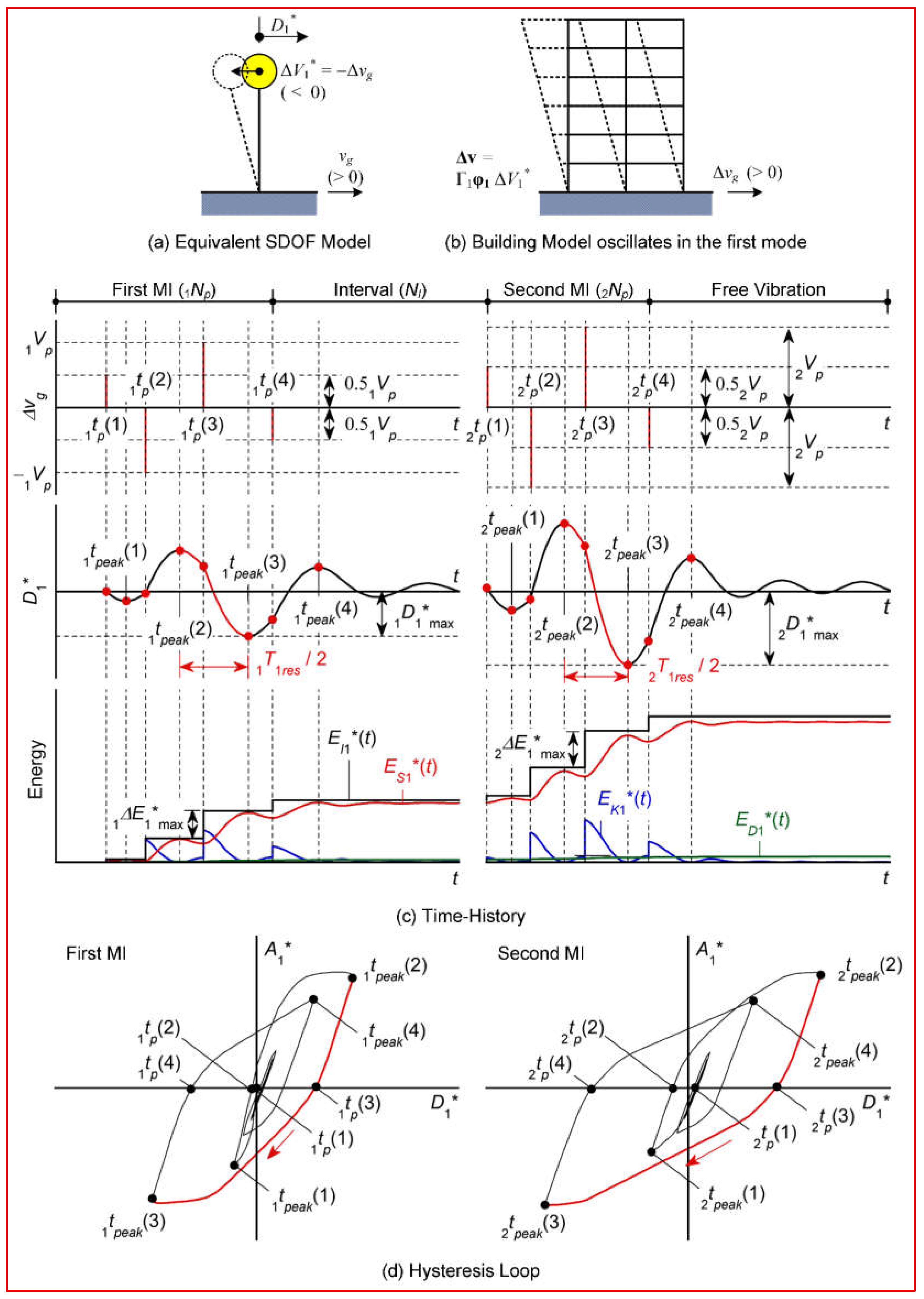
Figure 2.
Scheme to predict response of a structure under earthquake sequence.
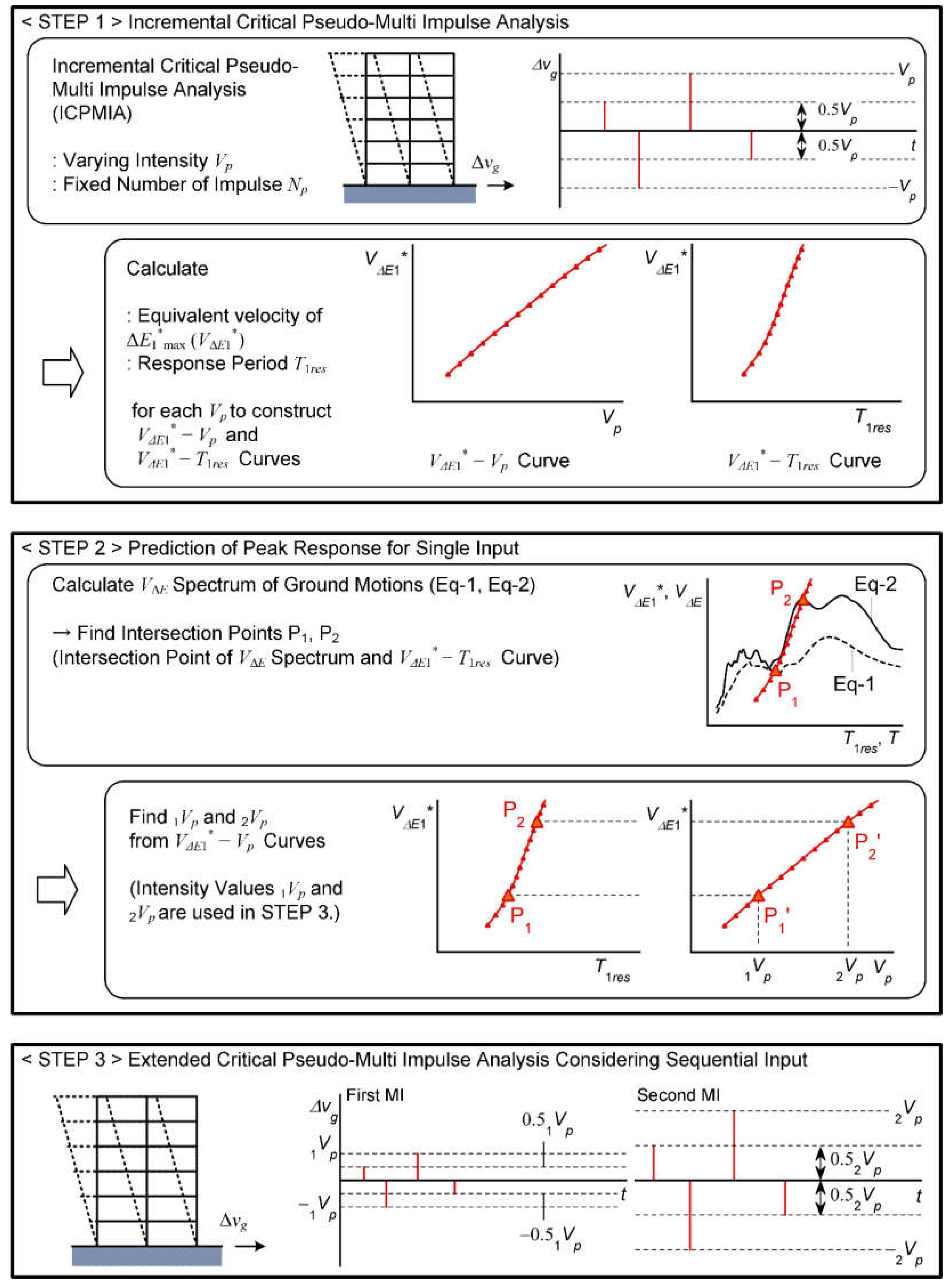
Figure 3.
Building model.
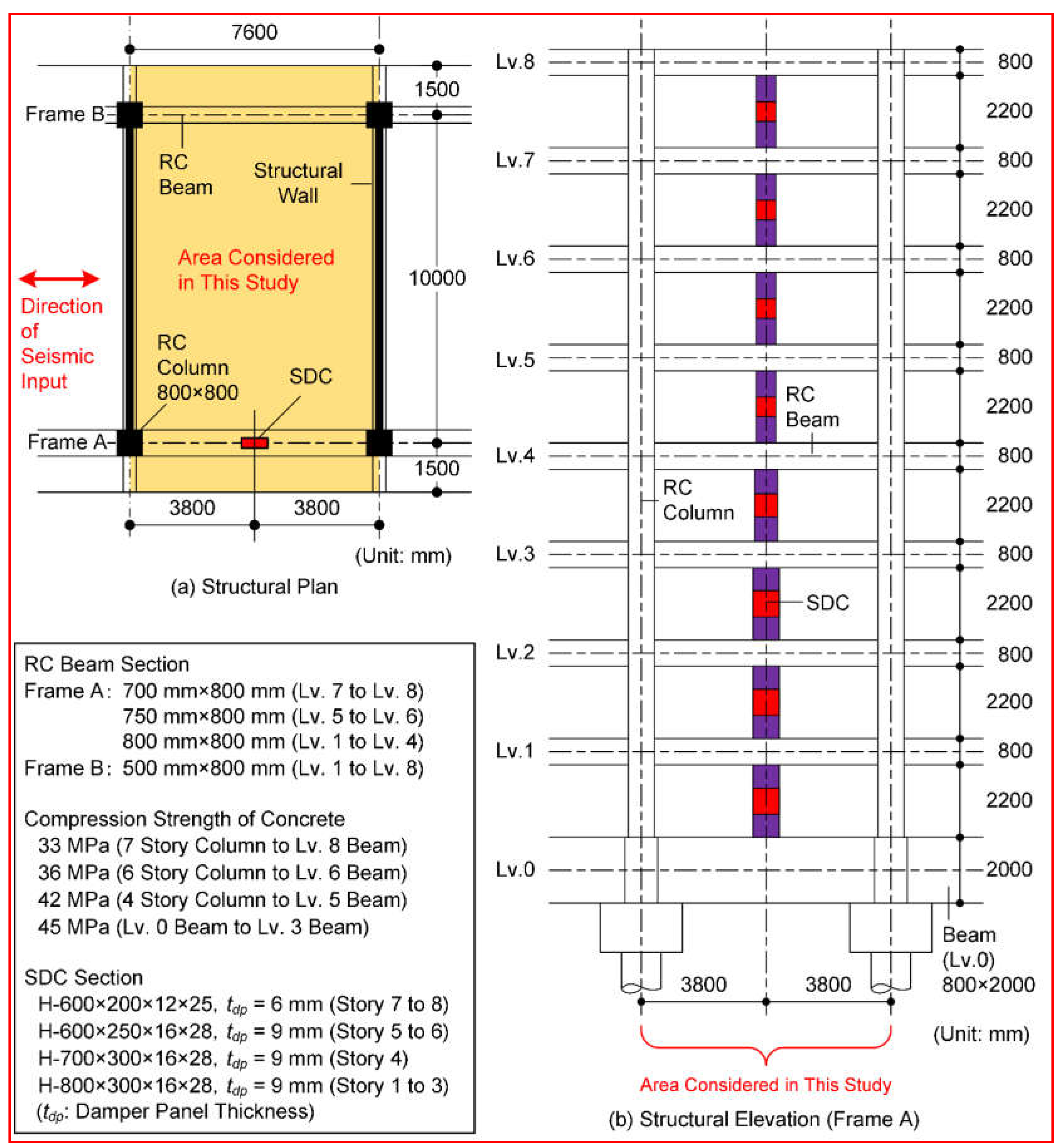
Figure 4.
Hysteresis rule of RC members and SDCs.
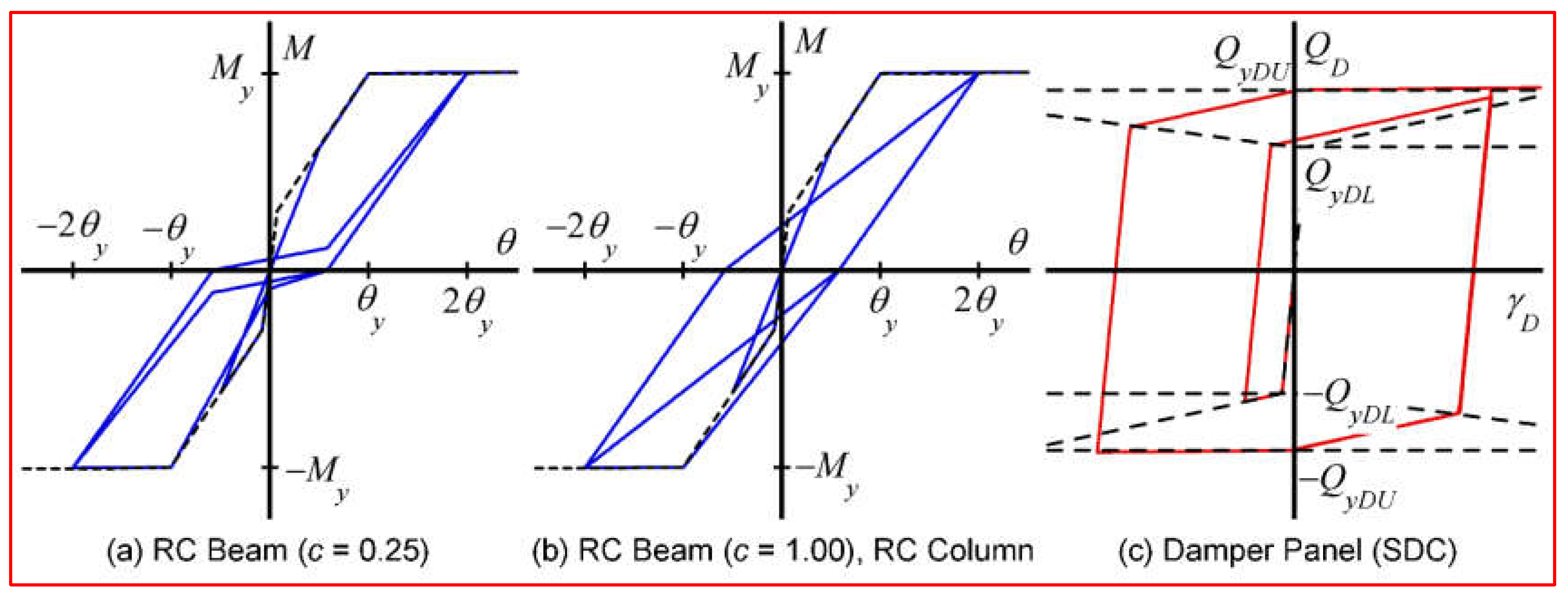
Figure 5.
VΔE and VI spectrum of ground motion set (complex damping: 0.10).
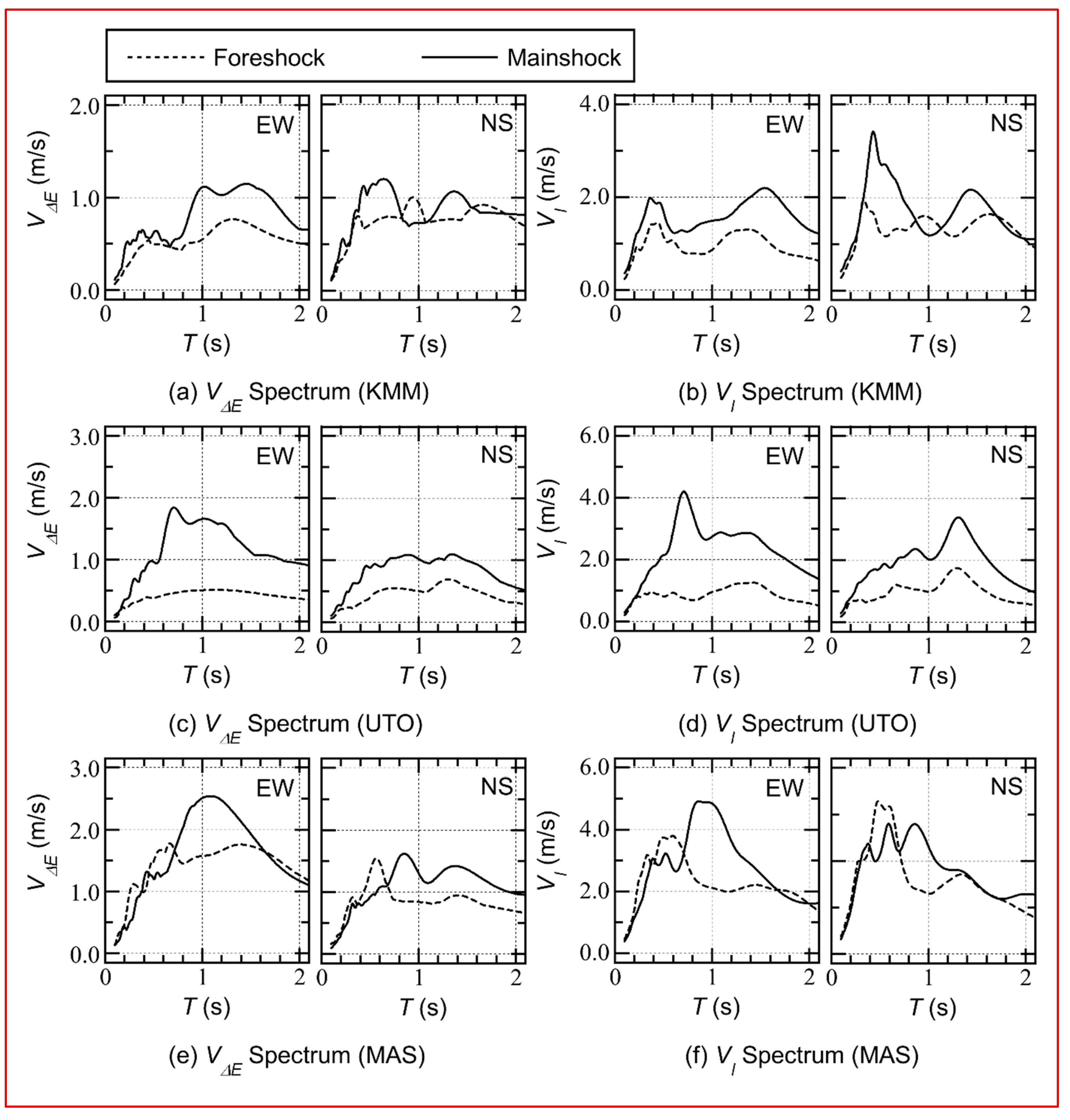
Figure 6.
Evaluation of 1Vp and 2Vp.
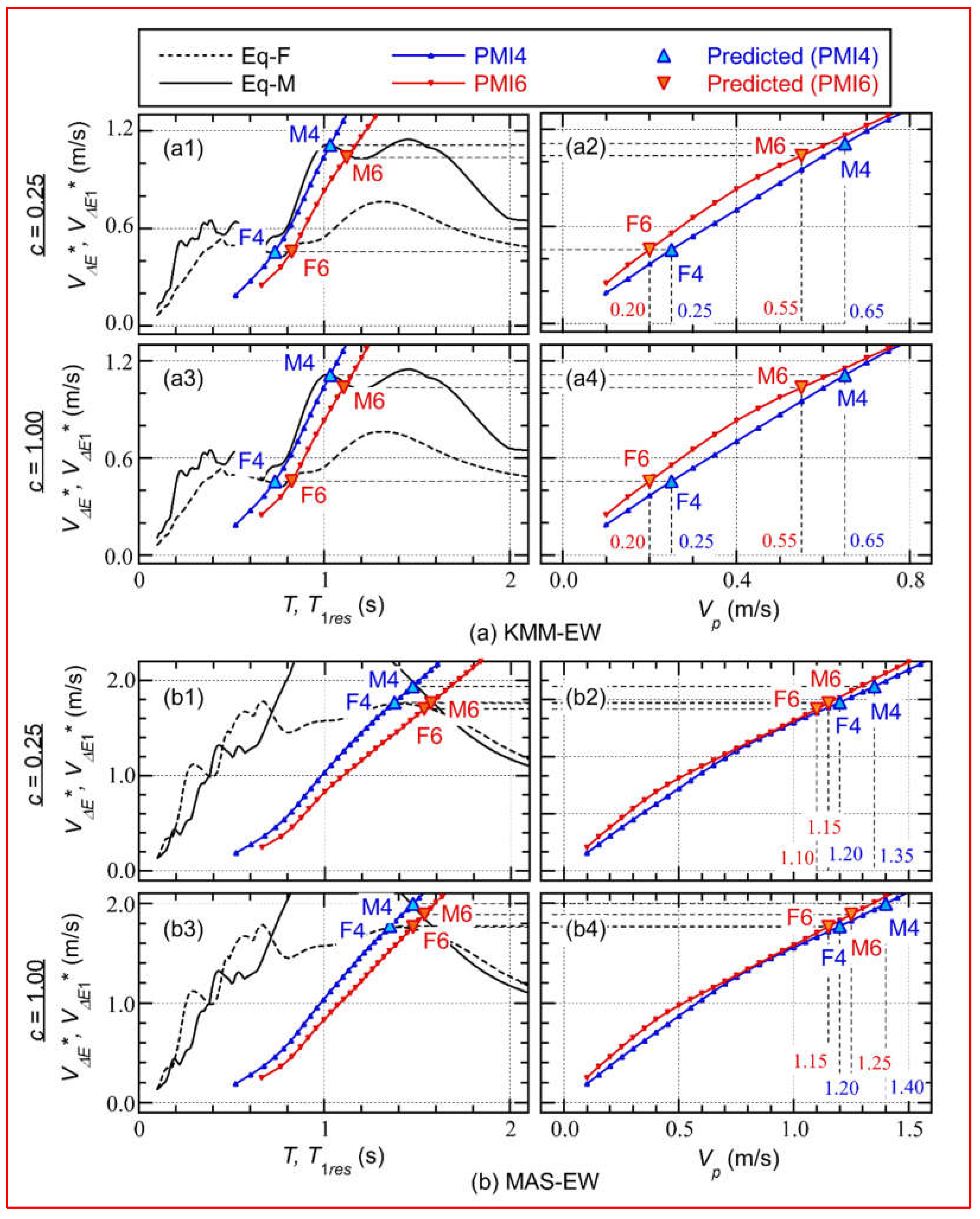
Figure 7.
Hysteresis loop obtained from PMI analysis.
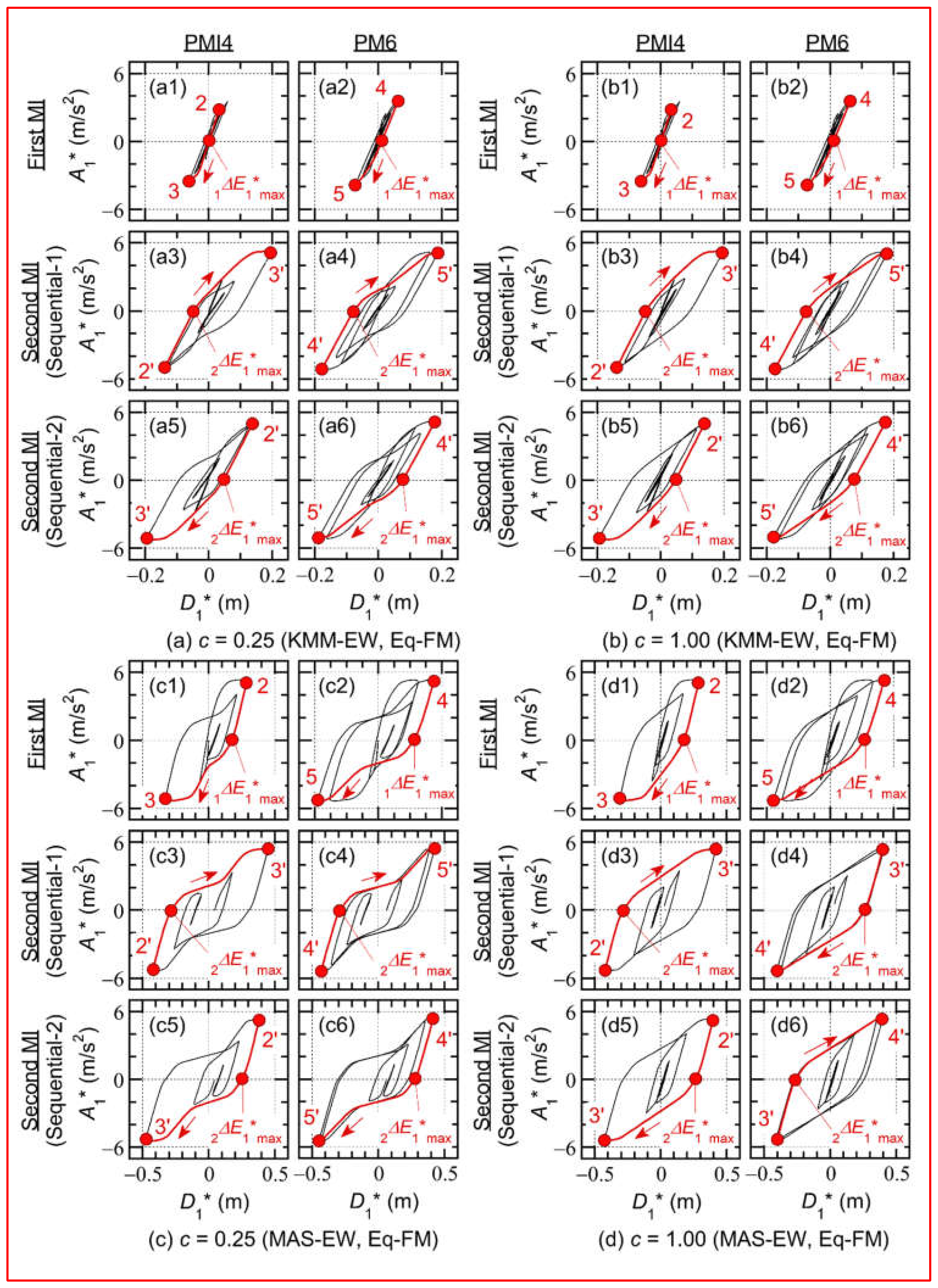
Figure 8.
Comparisons of cumulative energy.
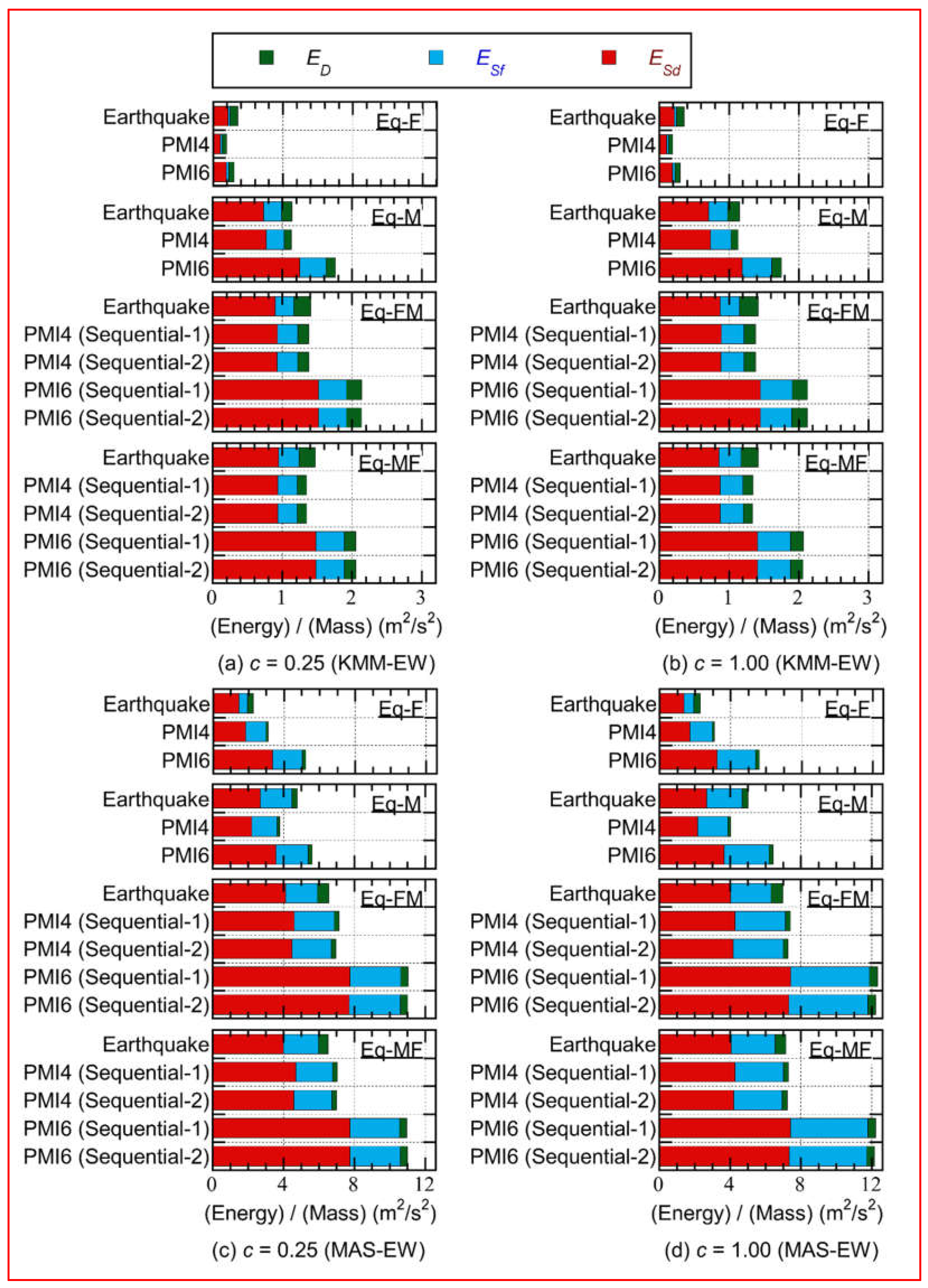
Figure 9.
Comparisons of local response (KMM-EW).
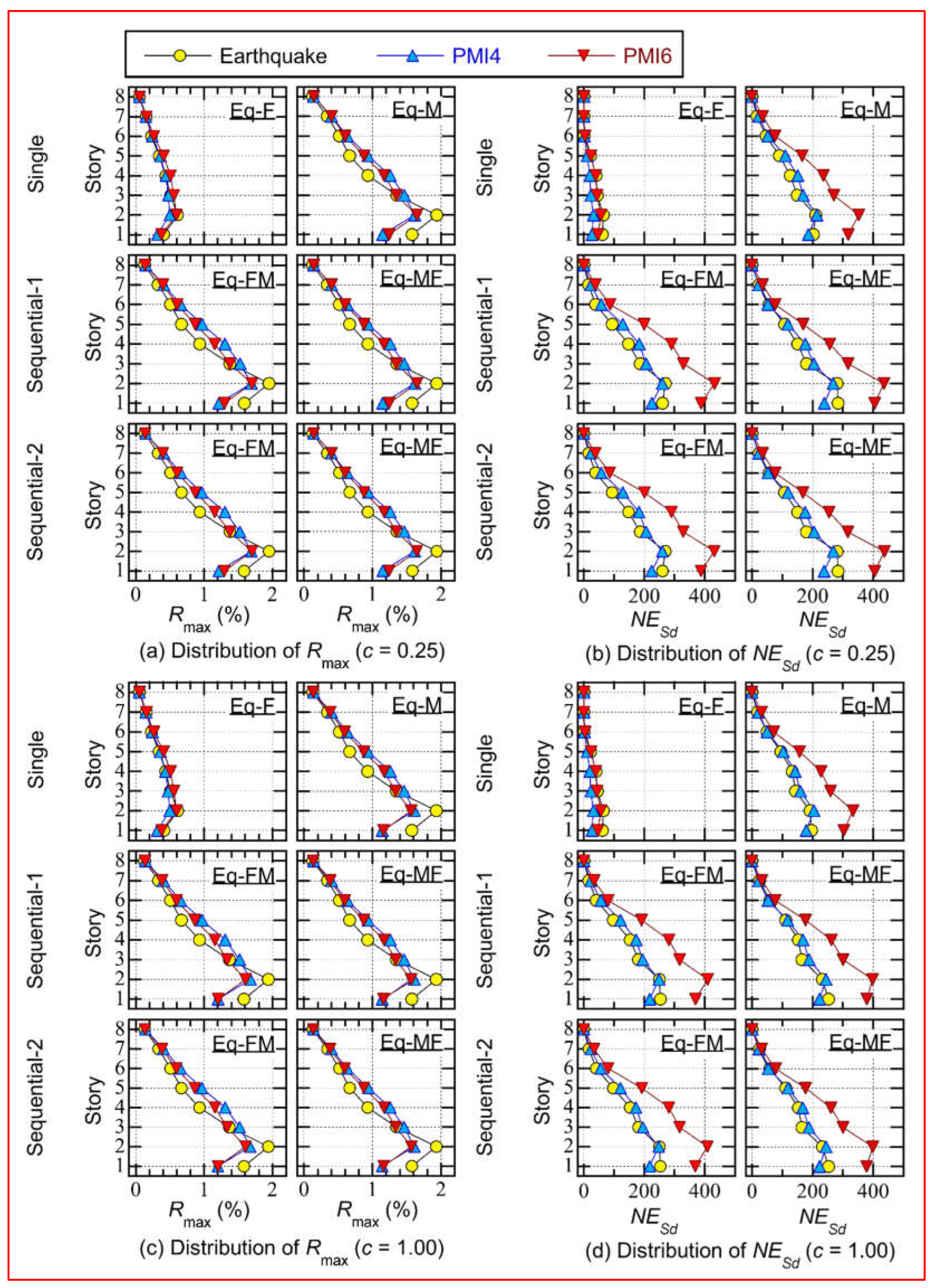
Figure 10.
Comparisons of local response (MAS-EW).
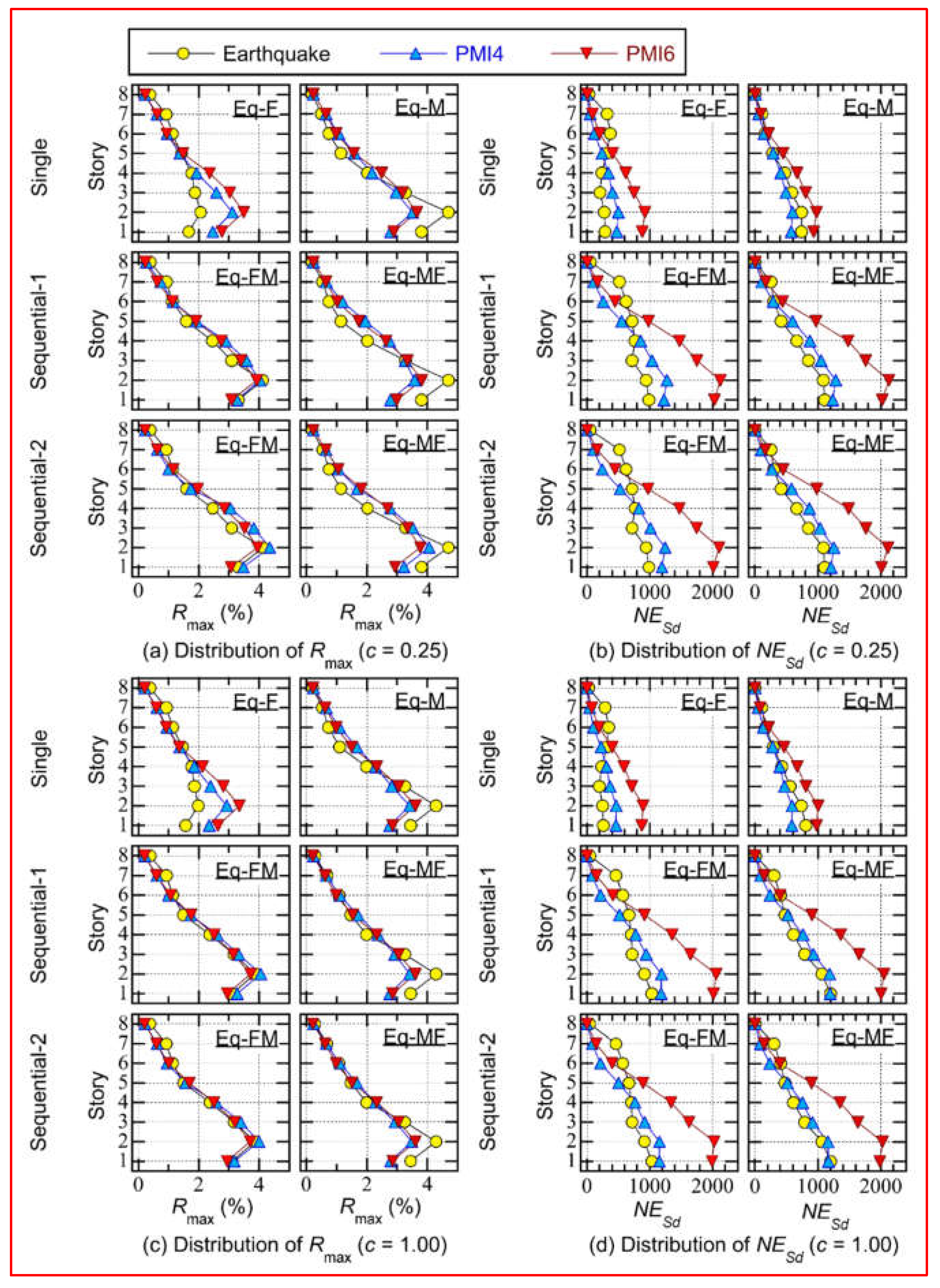
Figure 11.
Accuracy of the predicted VΔE1* and D1*max using critical PMI analysis.
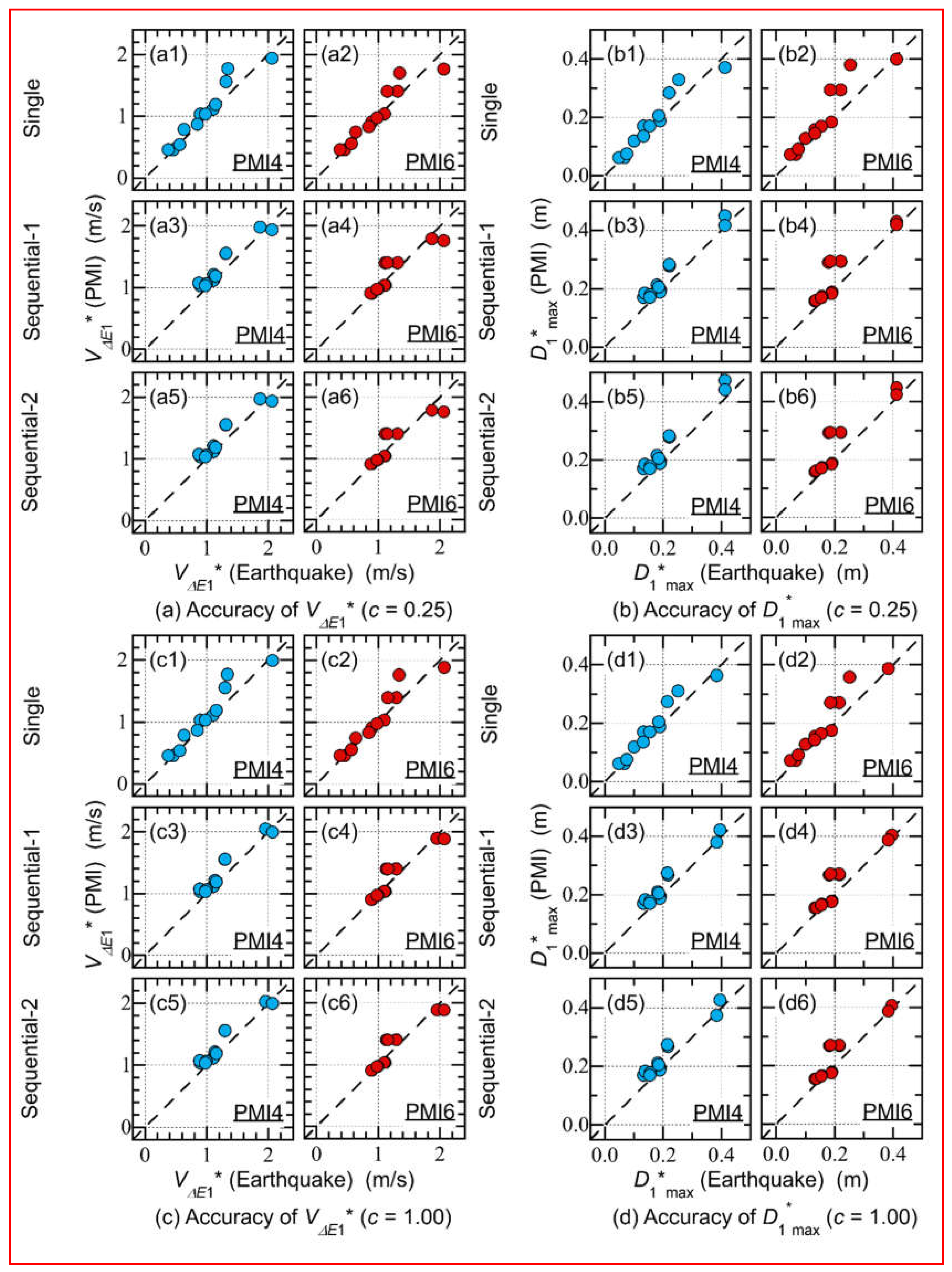
Figure 12.
Accuracy of the predicted cumulative strain energy using critical PMI analysis.
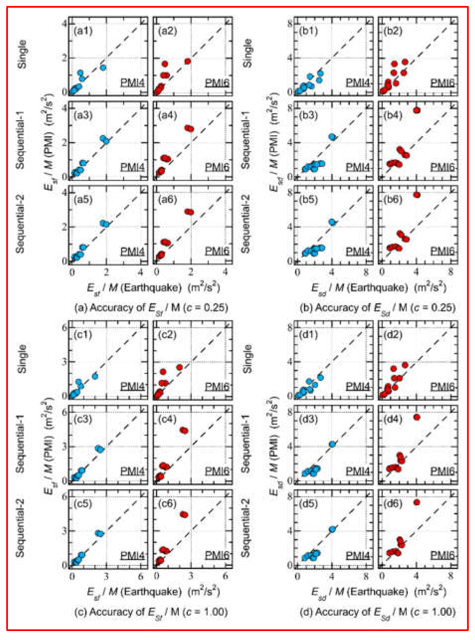
Figure 13.
Accuracy of the predicted local responses critical PMI analysis.
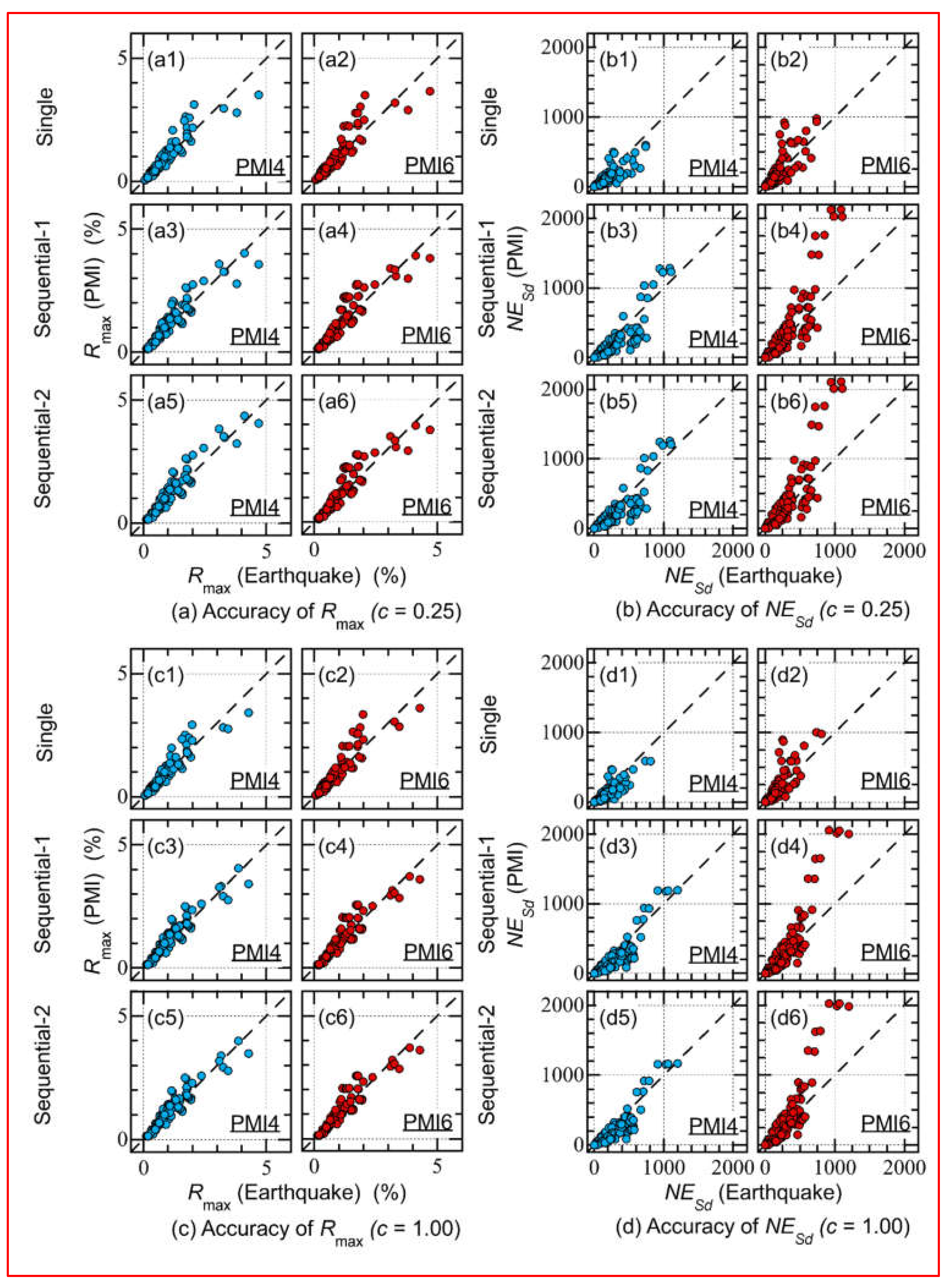
Figure 14.
VΔE1* - D1*max and VΔE1* - VI1* relationship.
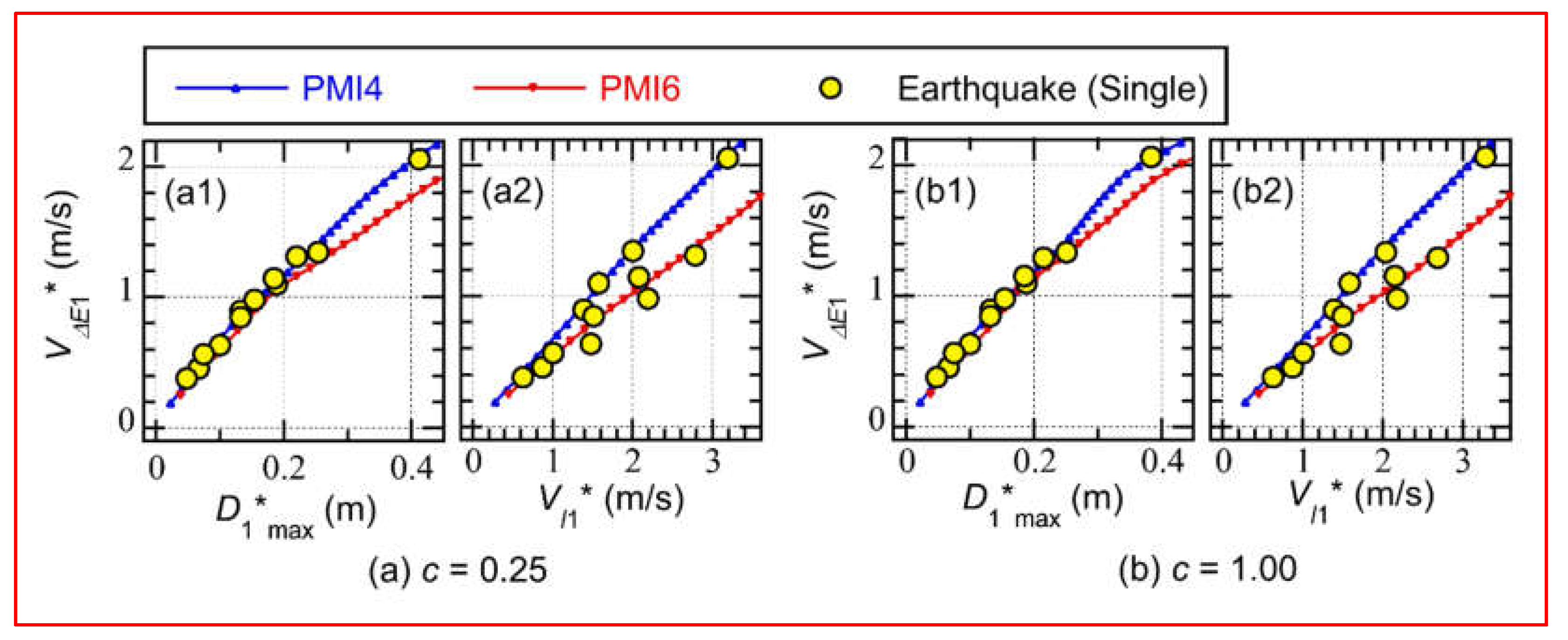
Figure 15.
Relationship between the (VΔE1* / VI1*) ratio obtained using recorded ground motions and that obtained from critical PMI analysis.
Figure 15.
Relationship between the (VΔE1* / VI1*) ratio obtained using recorded ground motions and that obtained from critical PMI analysis.
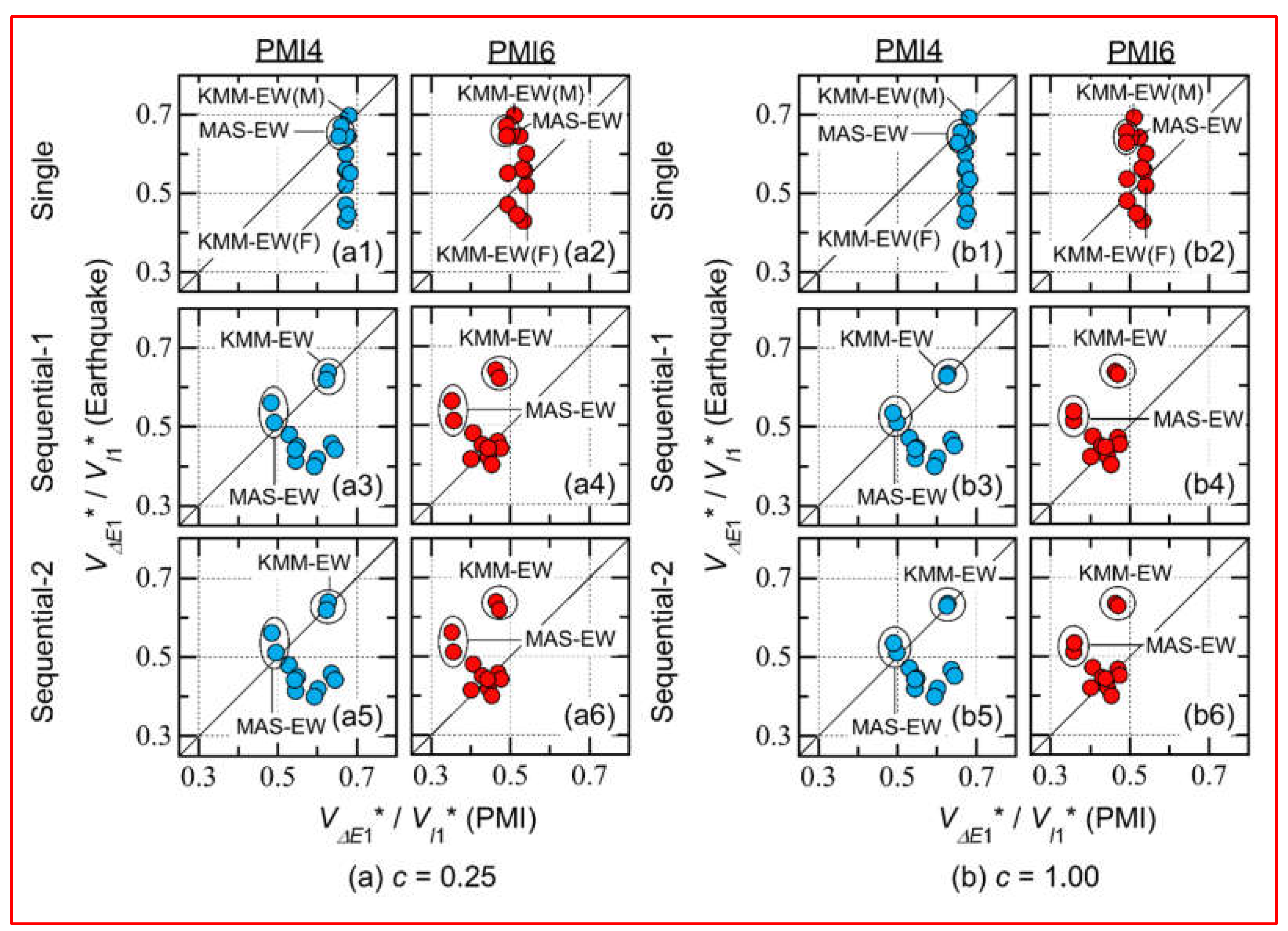
Disclaimer/Publisher’s Note: The statements, opinions and data contained in all publications are solely those of the individual author(s) and contributor(s) and not of MDPI and/or the editor(s). MDPI and/or the editor(s) disclaim responsibility for any injury to people or property resulting from any ideas, methods, instructions or products referred to in the content. |
© 2025 by the authors. Licensee MDPI, Basel, Switzerland. This article is an open access article distributed under the terms and conditions of the Creative Commons Attribution (CC BY) license (http://creativecommons.org/licenses/by/4.0/).
Copyright: This open access article is published under a Creative Commons CC BY 4.0 license, which permit the free download, distribution, and reuse, provided that the author and preprint are cited in any reuse.


