
Submitted:
11 March 2025
Posted:
12 March 2025
You are already at the latest version
Abstract
This two-parts paper is dedicated to the development of a pre-rationalization approach that provides favorable constructive properties for the low-tech construction of doubly curved structures. In part I, we provide methods for generating geometric constructs (patches) with two essential properties: One family of coordinate curves are planar (PU-property), while the other generating singly curved strips (develpable V-strips). The geometric constructs are done on three levels of geometric properties, of being: conjugate, orthogonal-conjugate (principal), and orthogonal-conjugate with negative constant Gaussian curvature (principal Tchebyshef nCGC). The main contribution of part I, is the articulation of a space of design variants within the pre-rationalization of the three levels, by introducing transforms leaving the geometric properties invariant, namely, Projective, Mo ̈bius, and Ba ̈cklund transforms.
Keywords:
Planar coordinate curves
; Developable strips
; Conjugate - Principal - Asymptotic Networks
; Projective - Mobius - Backlund transformations
; Fabrication-aware design
; Architectural geometry
1. Introduction
It is known that solutions for the construction methods of doubly curved gridshells can benefit a lot from the application of (discrete) differential geometry of curves and surfaces. In particular, extensive research in the relatively recent field of architectural geometry (cf. [1]) has brought to attention the important link between certain geometric properties and fabrication advantages. In this work, we focus on the following two geometric properties: PU-property and develpable V-strip. It is already brought to attention, cf. [2,3], that these two properties are significant.
As they provide important fabrication and structural advantages to gridshells construction. While in the mentioned works, the approach was more post-rationalization-based, in this paper, the approach is more pre-rationalization-based, using (smooth) surface typically parameterized by patches with coordinates . The PU-property requires all u-curves to be planar, while V-strip developability demands that the ruled strip formed by any two neighboring v-curves to be developable. The PU-property offers a reduction of falsework during construction, by using the planar u-curves as supporting structure, cf. [4,5,6].
This subject will be discussed in detail in part II of the paper. On the other hand, the developable V-strips enable cladding of the structure with laths that are simply bent with no torsion, cf. [7,8]. Furthermore, we observe that the three geometric levels in which the patches (having PU-property and developable V-strips) are defined, provide extra fabrication advantges as well. More precisely, conjugate patches give rise to planar panelling of the structure, since they are a smooth analog of PQ-meshes. Next, principal patches give rise to standard right-angled nodes and produce developable strips (generated by the surface normal along the network curves), allowing the carriers to be also made from simply bent laths with no torsion, cf. [9,10]. Finally, principal Tchebyshef nCGC patches come with corresponding asymptotic Tchebyshef nCGC patches, obtained by a simple reparameterizations, such that the two networks have matching intersection points. Hence, allowing for adding secondary bracing structures made by equal-length diagonals, cf. [11].
This subject will also be discussed in detail in part II of the paper. After defining the geometric constructs (patches with PU-property and developable V-strips) on the three levels, we provide associated transforms preserving these properties. The goal is to create a space of variants of design possibilities all having the fabrication advantages provided by the geometric properties.
Starting on level 1 (conjugate), all the defined geometric constructs are invariant under projective transforms. Next, on level 2 (principal), the defined geometric constructs are invariant under Möbius transforms (provided the u-curves are circular). Finally, on level 3 (principal nCGC) the defined geometric constructs (having PU-property and quasi-developable V-strips) are invariant under Bäcklund transforms. Illustrations are shown in Figure (Figure 1).
2. Geometry
In this section, we define the geometric constructs.
2.1. PU-Patches and Developable V-Strips
Let be the standard Euclidean scalar product on with its norm and × the cross product. In this paper, a curve is given by a smooth map and a surface by a smooth patch , both maps with values in . The derivatives of denoted by give rise to the curvature and torsion of the curve, denoted by . While the partial derivatives of X denoted by with its surface normal N, give rise to the fundamental coefficients and the Gaussian and Mean curvatures of the surface, denoted by , (for detailed formulas, cf. [12]). Recall that a patch is called conjugate if it satisfies everywhere. Next, by a PU-patch, we mean one for which all its u-curves are planar, i.e. having everywhere and by a V-strip we mean the ruled surface constructed by the joins of two neighboring v-curves:
for some fixed . In particular, if these strips satisfy having everywhere, then they are said to be developable. Clearly, the notions of a PV-patch and developable U-strip is analogous, hence will be omitted. Since we are interested in conjugate PU-patches with developable V-strips (because of their fabrication advantages, cf. Figure (Figure 1)), it is then useful to have simple conditions to characterize them. Now, applying the formula for torsion on u-curves of a patch X and the formula for Gaussian curvature on V-strips, we are able to formulate the following characterization. A patch X has:
for , and for any fixed and . Recall that, if X is conjugate, its V-strips are "quasi-developable", (), since, a developable strip is the smooth analog of a sequence of PQ-mesh faces, cf. [9,13,14,15].
2.2. Geometric Constructs on Three Levels
We construct PU-patches with developable V-strips.
• Level 1 - Conjugate: The archetypal patch in this level, is the Translation-type obtained by translating a planar generatrix curve along a (spatial) directrix curve , that is:
If the u-curves of a PU-patch are circular, then it is called a CU-patch, as seen in Figure (Figure 3). Note that, the Translation-type (3) is conjugate, satisfying Conditions (2), hence, is PU with developable V-strips.
• Level 2 - Principal: The second level of geometric constraint on our conjugate PU-patch X with developable V-strips, is requiring it to be orthogonal. This turns X into a principal patch, meaning, its coordinate -curves are curvature lines. This property adds further fabrication advantages, since any lath based on a strip obtained by sweeping the surface normal N along any coordinate curve is developable, cf. Introduction Section 1. The archetypal patch in this level, is the Revolution-type obtained by revolving a planar curve about an axis, that is:
This is clearly a CU-patch, as seen in Figure (Figure 4). The second patch example in this level, is obtained as the envelope of spheres, known as Dupin cyclide. Geometrically, this involves two quadratic curves called the focal directrices, on which the locus of centers of a family of spheres lie, cf. [16]. Now, when is an ellipse and is a hyperbola, we obtain an ellipto-hyperbolic cyclide, while, when are parabolas then we have a parabolic cyclide, as seen in Figure (Figure 5). The Cyclide-type is:
with , (for the first patch) and (for the second patch). Finally, it is directly verified that any patch X of Revolution-type (4) or Cyclide-type (5) has everywhere and satisfies Conditions (2). Hence, it is a principal PU-patch with developable V-strips.
The next patch on Level 2, is the Monge-type given by the union of (2 by 2) parallel curves (i.e. having the same normal planes at corresponding points) and their orthogonal trajectories. In more accurate terms, it is given by a family of planar generatrix curves drawn in the rectified normal planes along a spatial directrix curve . The rectification means rotating the normal and binormal vectors - generating the normal plane - of the directrix curve , about its tangent by, the torsion angle (integral of the torsion ), yielding . More precisely:
Note that by construction the v-curves are parallel curves, hence all the V-strips are developable.
The following patch on level 2, is Joachimsthal-type, it is given by a family of circular curves that are orthogonal trajectories to spherical curves, whose spheres’ centers lie on a straight line L. More precisely, it is given by the parameterization:
Note that, the vectors along any v-curve, generate a cone whose vertex o lies on the straight line L. Moreover, the v-curve is the intersection of the surface with a sphere centered at the point o, and cutting the surface orthogonally, as seen in Figure (Figure 7). We observe that any patch X of Monge-type (4) or Joachimsthal-type (5) is a principal PU-patch, cf. [17]. Moreover, if X is any Monge-type or any Joachimsthal-type (with ) then, the Condition (2)(2) is satisfied, turning the patch X into a principal PU-patch with developable V-strips.
The final example we present in level 2, is what we will call the Pencil-type. In this construction the desired PU-patch X is obtained from its spherical image N (i.e. surface normal), where the map N parameterizes a system of orthogonal circular arcs on the unit sphere. The circular arcs are in fact the intersections of two pencils of planes with the sphere, hence the name “pencil-type”. We observe that the spherical patch N arising in this way is conformal, with conformal factor , that is, its fundamental coefficients satisfy , and the patch X (from N) is given by the formula:
where the are functions u alone, resp. v alone. Note that, any patch X of Pencil-type (8) is principal with both its -curves planar, in other words, it is a PU-patch and a PV-patch. Notice, if then -curves are circular, as seen in Figure (Figure 8) and Condition (2)(2) is satisfied, hence X has developable V-strips. For a discrete construction of this, cf. [4,5].
• Level 3 - Principal nCGC: The third level of geometric constraints is to require our PU-patches to be principal with nCGC , with . The construction is based on principal Tchebyshef patches of radius and angle (half the angle between asymptotic directions). The fundamental coefficients satisfy , , and , with satisfying the Sine-Gordon Equation: . Moreover, a principal Tchebyshef patch has the property of being associated to an asymptotic Tchebyshef patch by the reparameterization . We will consider the four types: Pseudosphere-type (PS), Dini-type, Kuen-type, and Breather-type, obtained by Equation (11) (cf. [18]) yielding:
Each of the types above, is a principal patch that satisfies Condition (2)(1) making it a PU-patch, and, as a conjugate patch, it has quasi-developable V-strips.
2.3. Geometric Transforms on Three Levels
We construct geometric transforms preserving the geometric properties of the patches constructed above on the three levels. More precisely, we have the corresponding scheme:
• Level 1 - Projective transform: This is a bijective mapping of the projective space (seen as the lines through the origin in ), applied as multiplication by a regular ()-matrix on elements of . Upon seeing as the affine subspace , the projective transform of any patch , as seen in Figure (Figure 10), is given by:
Observe that, if the initial patch X is a conjugate PU-patch, then its projective transform will also be a conjugate PU-patch. This follows from the fact that, a projective transform preserves linear subspaces and conjugate patches, cf. [17,19]. Moreover, if the initial patch X is of a Translation-type (3), then its projective transform will satisfy Condition (2)(2), hence the developability of V-strips will be preserved as well.
• Level 2 - Möbius transform: This is a bijective mapping of the 3-sphere (seen as the compactification of ), cf. [20]. By restricting to , a Möbius transform can be given by compositions of translations, homotheties (uniform scaling), linear-orthogonal maps (Euclidean motion) and inversions. In more accurate terms, a Möbius transform of a patch , as seen in Figure (Figure 11), can thus be expressed by the formula:
Note that, if the initial patch X is a principal CU-patch, then its Möbius transform will also be a principal CU-patch. This follows from the fact that, a Möbius transform preserves circles and principal patches, cf. [17,19]. Furthermore, if we let in addition the initial patch X to have developable V-strips and also be any of the above defined types (geometric constructs): Revolution-type (4), Cyclide-type (5), Monge-type (6) (with circular), Joachimsthal-type (7) (with ), or Pencil-type (8) (with ). It then follows that, its Möbius transform will have developable V-strips as well. To see this, recall that developability is preserved by translation, homothety and linear-orthogonal maps. Thus, to conclude, we only need to verify that the inversion satisfy Condition (2)(2) in the stated types, which is indeed true.
• Level 3 - Bäcklund transform: This is a bijective mapping B between two surfaces of the same nCGC for some . Such that each line joining corresponding points is tangent to both surfaces, and has constant length , while the normals to both surfaces have a constant angle , as seen in Figure (Figure 12).
More analytically, a Bäcklund transform of X (a principal nCGC Tchebyshef patch of angle ) is:
Starting with a degenerate patch (with ), applying Bäcklund transform with generic inclination yields the Dini-type, while applying it with yields PS-type and upon second application with yields Kuen-type (for more details cf. [18]).
2.4. Extra Possibilities
We can also mix levels of transforms and properties to increase the design options by extra possibilities.
• Extra possibilities - Projective transform: Applying a projective transform to a principal CU-patch, yields a conjugate PU-patch. If in addition the initial patch has developable V-strips and is: Revolution-type (4), Cyclide-type (5), Joachimsthal-type (7) (with ), Pencil-type (8) (with ), its projective transform also has developable V-strips.
• Extra possibilities - Möbius transform: Applying a Möbius transform to a principal nCGC Tchebyshef PU-patch, yields a principal patch with spherical u-curves. In fact, a Möbius transform of a conjugate CU-patch is just a CU-patch, while a Möbius transform of a principal PU-patch of Monge-type (6) or Pencil-type (8), is just a principal patch.
• Extra possibilities - Bäcklund transform: Observe that using the parameter w appearing in the expressions of the Kuen-type, as a coordinate, yields a 3-dimensional patch , parameterizing a triply orthogonal system of surfaces (TOS) called Ribaucour TOS (R-TOS). Note that, patches are principal nCGC Tchebyshef PU-patches, while the patches and are principal with w-curves circular, for any fixed . Up to renaming parameters, the principal patches will be considered CU-patches with developable V-strips (which we will call R-TOS-Type). The same goes for their Möbius transforms, as seen in Figure (Figure 14).
3. Morphology
In this section, we will focus on the application of the geometric constructions in design morphology. This implies showing how these geometric constructs and their transforms can be readily utilized within pre-rationalized design approach. These are formulated through explicit parametrizations with multiple parameters, that can thus be used for different designs by changing their respective input values. It is clear that, an infinite number of variants of a given geometric construct and its transform (all sharing the same geometric properties and fabrication advantages) can be generated by varying these parameters. For sake of clarity, we also provide an overview of the different combinations of transforms and geometric constructs in Figures (Figure 15) and (Figure 16). This can be seen as a visual summary of the geometric results of Section 2.
This parametric approach allows us to define a broad search space of design variants (all having the desired geometric properties), that will be referred to as the Space of Variants. Establishing this space is a crucial step in "translating" geometry into architectural design morphology.
The morphological exploration of the space of variants revolves around two primary Degrees of Design Freedom (DF) (this concept was introduced by some of the authors in [21,22,23]). The DF can subdivided into:
It is evident that DF-1, which involves selecting the geometric construct (i.e. patch-type), determines the starting level (i.e. level 1, 2 or 3). However, DF-2 allows us to either remain at the same level or transition to another level. For instance, choosing the geometric construct to be of Revolution-type, places us on level 2 (principal). Next, applying a Möbius transform will keep us on level 2, while applying a projective transform will moves us down to level 1 (conjugate), as illustrated in Figure (Figure 16). It is clear that, the choices in DF-1 and DF-2 are influenced by the fabrication method and materials specific to each project. This relationship underscores how each level is associated with distinct fabrication advantages, as discussed in the Introduction Section 1 in Figure (Figure 1).
3.0.1. Encoding the DF information
To track the variants, each one can be assigned an “ID-code” reflecting the “path” it took in the space of variants, i.e. its DF-1 and DF-2 information. The DF-1 part includes the patch-type (typ) and patch-parameters (abc000) and the DF-2 part includes the transform-type (TYP) and transform-parameters (ABC000). Finally, the three colors indicate the three levels of the geometric constructs, as shown in Figure (Figure 17). This method can be useful to navigate the space of variants during morphological exploration.
3.1. Space of Variants - Construction
In the previous paragraph, we discussed the possible combinations in the space of variants, presenting their possible DF-1 and DF-2 choices or “paths”. To illustrate their parametric design capabilities, let us now provide concrete examples of how the DF-1 and DF-2 choices are implemented using explicit parameterizations of the geometric constructs (belonging to the three levels). It is clear that choosing different functions in the constructions in Section 2 will result in different paramterizations. We choose the following ones to simply make clear the ideas and showcase the parameteric approach. We now choose the following three explicit parameterizations:
• Level 1: We will choose the geometric construct X to be of Translation-type generated from the specific planar curve and the spatial curve , given by:
The input patch-parameters generate DF-1 and the patch X defined by Equation (3), takes on the explicit parameterization form:
• Level 2: We will choose the geometric construct X to be of Pencil-type, generated from a specific conformal patch N on the unit sphere with the conformal factor , and the function , given explicitly by the formulas:
The parameters are input patch-parameters that make DF-1, and the patch X by Equation (8) takes on the explicit parameterization form:
• Level 3: We will choose the geometric construct X to be of Dini-type, generated as a Bäcklund transform (11)(1) of the vertical line , with respective angle functions satisfying the Bäcklund-Darboux Equations (11)(2), and given by:
The parameters are its input patch-parameters making DF-1 and the patch X defined by Equation (11) takes on the explicit parameterization form:
Now that we have our explicit geometric constructs (from each level), we are ready to augment DF-1 with DF-2, that is, applying geometric transforms to these patches. As mentioned above, for the exploration within DF-2, we use projective, Möbius and Bäcklund transforms. Recall that the projective transform is defined by Equation (9) with input parameters ’s. In particular, by changing their values, we can obtain different projective transforms (of the initial patch) and hence a design exploration in DF-2. Next, in our presented example, we will define a Möbius transform given by a composition of inversion, then translation by a vector , followed by second inversion. This is because inversions have the most significant impact on the shape, thus are more important for design exploration. In this presented Möbius transform example, the parameters determine the inversion, and each set of input values will yield a different Möbius transform (of the initial patch) and hence a design exploration in DF-2. Finally, the Df-2 on level 3 is established by the application of the Bäcklund transforms. Note that, this is a special case, as the parameterizations of the geometric constructs (principal nCGC Tchebyshef patches) are themselves Bäcklund transforms. Consequently, parameters can be interpreted as generating DF-1 or DF-2. For example, the parameterization of the Kuen-type involves parameters . From one side, these are patch-parameters (i.e. DF-1) while from another side, they are transform-parameters (i.e. DF-2) because Kuen-type is a Bäcklund transform of the PS-type.
3.2. Space of Variants - Exploration
We first explore the space of variants through DF-1.
• Varying patch-parameters (tra): For the Translation-type patch X given by Expression (12), where we have patch-parameters . We fix all parameters and we vary the parameter l and then parameter f, as seen in Figure (Figure 18).
• Varying patch-parameters (pen*): For the Pencil-type patch X given by Expression (13), where we have patch-parameters . We again fix all parameters and we vary the parameter o and then parameter k, as seen in Figure (Figure 19).
• Varying patch-parameters (din): For the Dini-type patch X given by Expression (14), where we have patch-parameters . Once again to demonstrate the morphological effect more clearly, we fix all parameters and we vary the parameter s and then parameter w, as seen in Figure (Figure 20).
Observe that, on level 1 (conjugate), we start by a Translation-type patch (tra) having PU-property and developable V-strips and so do all of its variations, as seen in Figure (Figure 18). Here, we have the fabrication advantage of having planar carrier beams (from the u-curves) and cladding by developable strips (from V-strips). Next, on level 2 (principal), we start by a Pencil-type patch (pen*) having PU-property and developable V-strips and so do, all of its variations. Here, the carrier beams (in both directions) can be made from laths based on developable strips (generated by surface normals), with orthogonal connection nodes, as seen in Figure (Figure 19). Finally, on level 3 (principal Tchebyshef nCGC), we start by a Dini-type patch (din) having PU-property and quasi-developable V-strips and so do, all of its variations. Besides, the developablility of the laths making the carrier beams (from -curves), we have here the fabrication advantage of having a bracing substructure beams based on asymptotic curves. Thus, can be made from straight laths, that in particular, have equal-length diagonals intersecting the main structure (by principal curves), as seen in Figure (Figure 20). Let us now explore the space of variants through DF-2.
• Varying transfrom-parameters (PRJ): We will now apply a projective transform to the Translation-type patch X, yielding the transformed patch given by Expression (9), where we have transform-parameters . We fix all the parameters and vary the parameter (denoted by ) and then parameter (denoted by ), as seen in Figure (Figure 21).
• Varying transfrom-parameters (MOB): We now apply a Möbius transform to the Pencil-type patch X, yielding the transformed patch given by Expression (10). In here, the transform-parameters are the coordinates . We vary the parameters (denoted by A), then (denoted by B) and finally (denoted by C), as seen in Figure (Figure 22).
• Varying transfrom-parameters (BAC): Finally, we will apply a Bäcklund transform (with complex inclination) to the Dini-type patch X, yielding the transformed patch Breather-type patch. In here, the transform-parameters are (with ). As before, we fix all parameters, and we vary the parameter d (denoted by D), as seen in Figure (Figure 23).
To end this section, we would like to point out some remarks, regarding the 3D-modeling of the mathematical surfaces. Observe that, the explicit analytic expressions obtained by the geometric processes described in DF-1 and DF-2 are evaluated at discrete number of points (in the domain) yielding discrete number of points that are exactly on the surface. Next, interpolations (based on NURBS) of these points create approximations of the mathematical surface. Clearly, the higher the number of evaluation points, the better the NURBS approximations (of the mathematical surfaces) are, and hence the more accurate the desired geometric properties are. Once the final shape (NURBS) is fixed, standard architectural 3D-modeling processes are then applied to model the fabrication elements. Namely, the nodes, beams and panels, in particular giving them thicknesses (usually from normals of the NURBS surface). Now, issues regarding accuracy of the geometric properties (e.g. planarity, developability) of these elements may arise, if we have an insufficient number of evaluation points. This error tolerance is naturally adjusted to each project, by using more evaluation points.
4. Case-Study: Dini-Type Patch
Let us end this part I of the paper, by focusing on a specific patch-type from level 3, namely the Dini-type patch. This will be used as the geometric basis for the realized structure in part II. We saw above that, it satisfies the PU-property and V-strip quasi-developability. Let us now discuss some of its other important geometric properties.
• Corresponding Principal-asymptotic networks: We recall that, as a principal Tchebyshef nCGC patch, our Dini-type patch given by the Expression (14), comes with a corresponding “diagonal” asymptotic Tchebyshef nCGC patch given by , that is:
The fundamental coefficients satisfy the conditions: , and , where the angle (equals ) satisfying the Sine-Gordon equation . In more concrete terms, the principal Dini-type patch and the asymptotic Dini-type patch naturally give rise to networks of principal and asymptotic curves respectively. Next, we select a discrete number of -curves and -curves, each equally spaced (along the two variables) in their respective domains. It will then follow, that the induced principal and asymptotic networks will correspond, in the sense that their intersection points will perfectly match with each other, as seen in Figure (Figure 24).
• Floral appearance: Another important (aesthetic) feature of the Dini-type patch, which was in fact a main motivation for its selection to be used as the geometric basis for the realized structure explained in part II, is its "floral" appearance, as seen in Figure (Figure 25). Since this project was part of a plant-themed exposition Plant Fever, the floral character provided by the Dini-type patch made it very suitable for such an application. More on this, in part II of the paper.
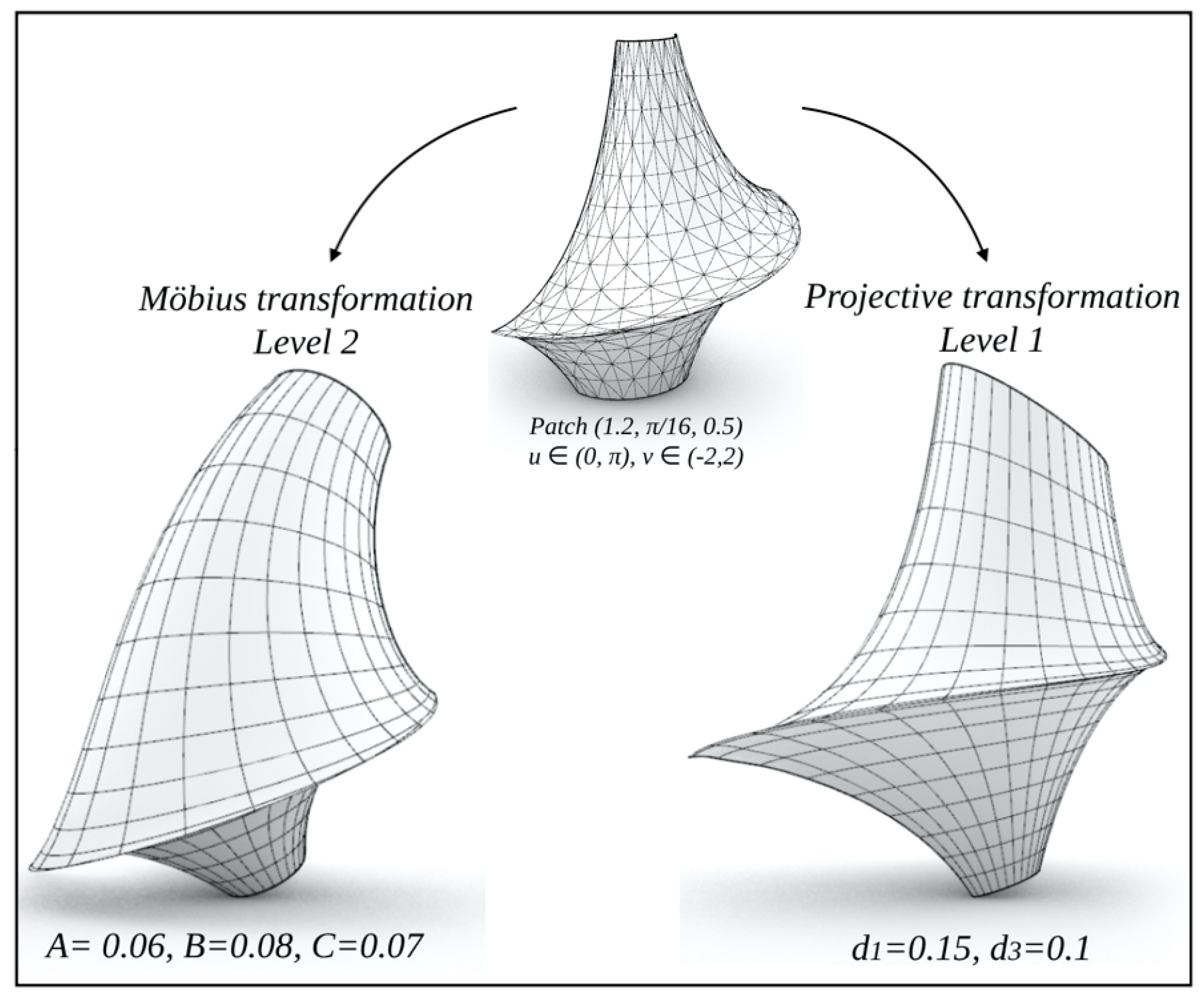
• Projective and Möbius transforms: To finish, let us illustrate the application of projective and Möbius transforms to the Dini-type patch, as seen in Figure (Figure 16). Since the Dini-type patch is a principal (i.e. orthogonal-conjugate) nCGC PU-patch, its projective transform will be a conjugate PU-patch, however it will no longer be orthogonal nor nCGC. On the other hand, its Möbius transform will remain principal but will no longer be nCGC nor satisfy the PU-property, as seen in Figure (Figure 26).
5. Conclusions
To conclude part I of the paper, we would like to make some summarizing remarks, regarding our (research) method and its application potential in the field of doubly curved gridshells. To begin, we recall that this (two-part) paper investigates a mathematical approach to the design of doubly curved structures (gridshells), from conception to construction, which is referred to as the pre-rationalization approach. The prefix "pre" indicates that the choice of geometric properties, or “rationalization” is determined beforehand, and then morphological exploration of the design options is done through (parameters variations and) transformations, that leave these geometric properties invariant. For this particular paper, we focused on ensuring that the geometric constructs (i.e. patch-types) possess two fundamental basic properties, namely the PU-property and V-strips developability, each with fabrication advantages shown above. Moreover, the geometric constructs that satisfy these two properties were constructed on three levels of additional geometric constraints, namely being conjugate, principal, and principal (Tchebyshef) nCGC. On one side, these additional geometric constraints facilitated the mathematical construction of the patches in question, and on the other side, these extra properties provided other fabrication advantages that were explained above, cf. Introduction Section 1. These geometric constructs and their transforms can be used as efficient geometric bases for the design and construction of gridshells, that is low-tech and with less false-work. To illustrate this, a geometric construct (Dini-type patch) will be the basis for a realized structure that will be elaborated in part II of the paper. Perhaps, it is worth mentioning that, even though the Dini-type patch has only quasi-developable V-strips, it is still a justifiable choice. This is because, on one hand, in practice, the error of quasi-developability is completely within the architectural application tolerance, and on the other hand, being from level 3, it provided us the principal-asymptotic networks correspondence, which is a greater fabrication benefit. In closing, we hope that the methods presented, were clear for designers (and non-mathematical readers) to readily use and that they stimulate further research in mathematical application in gridshells design.
Acknowledgments
The research of the author Tošić, Z. is part of the priority program SPP 2187 and funded by the German Research Foundation (DFG) and the research of the author Elshafei, A. was partially financed by Portuguese Funds through FCT (Fundação para a Ciência e a Tecnologia) within the Project UIDB/00013/2020 and the project UIDP/00013/2020.
References
- Pottmann, H. Architectural Geometry and Fabrication-Aware Design. Nexus Network Journal 2013, 15, 195–208. [Google Scholar] [CrossRef]
- Pottmann, H.; Schiftner, A.; Bo, P.; Schmiedhofer, H.; Wang, W.; Baldassini, N.; Wallner, J. Freeform surfaces from single curved panels. ACM Transactions on Graphics 2008, 27, 1–10. [Google Scholar] [CrossRef]
- Verhoeven, F.; Vaxman, A.; Hoffmann, T.; Sorkine-Hornung, O. Dev2PQ: Planar Quadrilateral Strip Remeshing of Developable Surfaces 2021.
- Tellier, X.; Douthe, C.; Hauswirth, L.; Baverel, O. Surfaces with planar curvature lines: discretization, generation and application to the rationalization of curved architectural envelopes. Automation in Construction, Elsevier 2019, 106, 102880. [Google Scholar]
- Mesnil, R.; Douthe, C.; Baverel, O.; Leger, B. Morphogenesis of surfaces with planar lines of curvature and application to architectural design. Automation in Construction, Elsevier 2018, 95, 129–141. [Google Scholar] [CrossRef]
- Wang, C.; Jiang, C.; Wang, H.; Tellier, X.; Pottmann, H. Architectural Structures from Quad Meshes with Planar Parameter Lines. Computer-Aided Design 2023, 156, 103463. [Google Scholar] [CrossRef]
- Synthesis of Strip Pattern Project. Synthesis of Strip Pattern. https://www.me-st.com/Synthesis-of-Strip-Pattern, n.d. Synthesis of Strip Pattern Project. Synthesis of Strip Pattern. https://www.me-st.com/Synthesis-of-Strip-Pattern, n.d. Accessed: 2024-08-14.
- Stanojevic, D.; Takahashi, K. Strip-Based Double-Layered Lightweight Timber Structure. In Proceedings of the Proceedings of IASS Annual Symposia.; IASS 2019 Barcelona Symposium: Elastic Gridshells and Bending Active Systems, 2019. [Google Scholar]
- Bobenko, A.; Tsarev, S. Curvature line parameterization from circle patterns. available from arXiv: 0706.3221, arXiv:0706.3221 2007.
- Pottmann, H.; Liu, Y.; Bobenko, A.; Wallner, J.; Wang, W. Geometry of multi-layer freeform structures for architecture. ACM Tr., Proc. SIGGRAPH 2007, 26, 1–11. [Google Scholar]
- Pottmann, H.; Wallner, J. The focal geometry of circular and conical meshes. Advances in Computational Mathematics 2008, 29, 249–268. [Google Scholar]
- Gray, A.; Abbena, E.; Salamon, S. Modern differential geometry of curves and surfaces with Mathematica. Third Edition; Chapman & Hall / CRC, 2006.
- Bobenko, A.; Suris, Y. Discrete differential geometry. Consistency as integrability. available from arXiv:math/0504358.
- Liu, Y.; Pottmann, H.; Wallner, J.; Yang, Y.; Wang, W. Geometric modeling with conical meshes and developable surfaces. ACM Tr., Proc. SIGGRAPH 2006, 25, 681–689. [Google Scholar] [CrossRef]
- Pottmann, H.; Schiftner, A.; Bo, P.; Schmiedhofer, H.; Wang, W.; Baldassini, N.; Wallner, J. Freeform surfaces from single curved panels. ACM Tr. 2008, 27, 1–10. [Google Scholar]
- Ferréol, R. Encyclopédie des formes mathématiques remarkables; https: //mathcurve.com, 2017. [Google Scholar]
- Eisenhart, L. A Treatise on Differential Geometry of Curves and Surfaces; Ginn and Company: Boston, 1909. [Google Scholar]
- Rogers, C.; Schief, W.K. Bäcklund and Darboux transformations: Geometry and modern applications in soliton theory; Cambridge university press: Cambridge, 2002. [Google Scholar]
- Eisenhart, L.P. Transformations of Surfaces; Princeton university press: Princeton, 1923. [Google Scholar]
- Cecil, T.E. Lie Sphere Geometry and Dupin Hypersurfaces. Mathematics Department Faculty Scholarship 2018. [Google Scholar]
- Abdelmagid, A.; Elshafei, A.; Mansouri, M.; Hussein, A. A Design Model for a (Grid)shell Based on a Triply Orthogonal System of Surfaces. Proceedings of Design Modelling Symposium Berlin, Springer, 2022; 46–60. [Google Scholar]
- Mansouri, M.; Abdelmagid, A.; Tosic, Z.; Orszt, M.; Elshafei, A. Corresponding principal and asymptotic patches for negatively-curved gridshell designs. Proceedings of Advances in Architectural Geometry, DeGruyter, 2023; 55–67. [Google Scholar]
- Abdelmagid, A.; Tosic, Z.; Mirani, A.; Hussein, A.; Elshafei, A. Design Model for Block-Based Structures from Triply Orthogonal Systems of Surfaces. Proceedings of Advances in Architectural Geometry, DeGruyter, 2023; 165–176. [Google Scholar]
Figure 1.
Translating geometric properties to fabrication advantages.
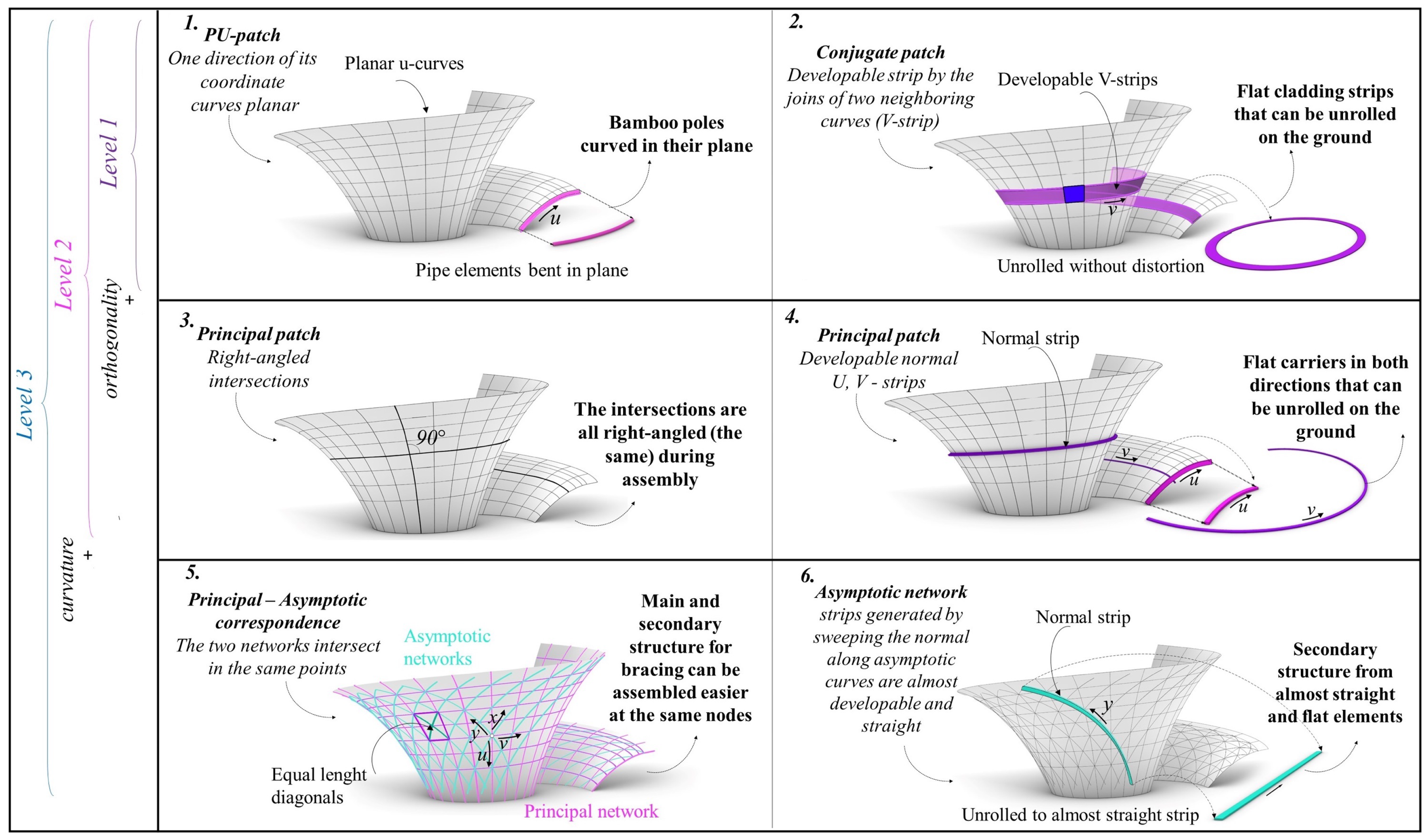
Figure 2.
Developability of V-strips condition.
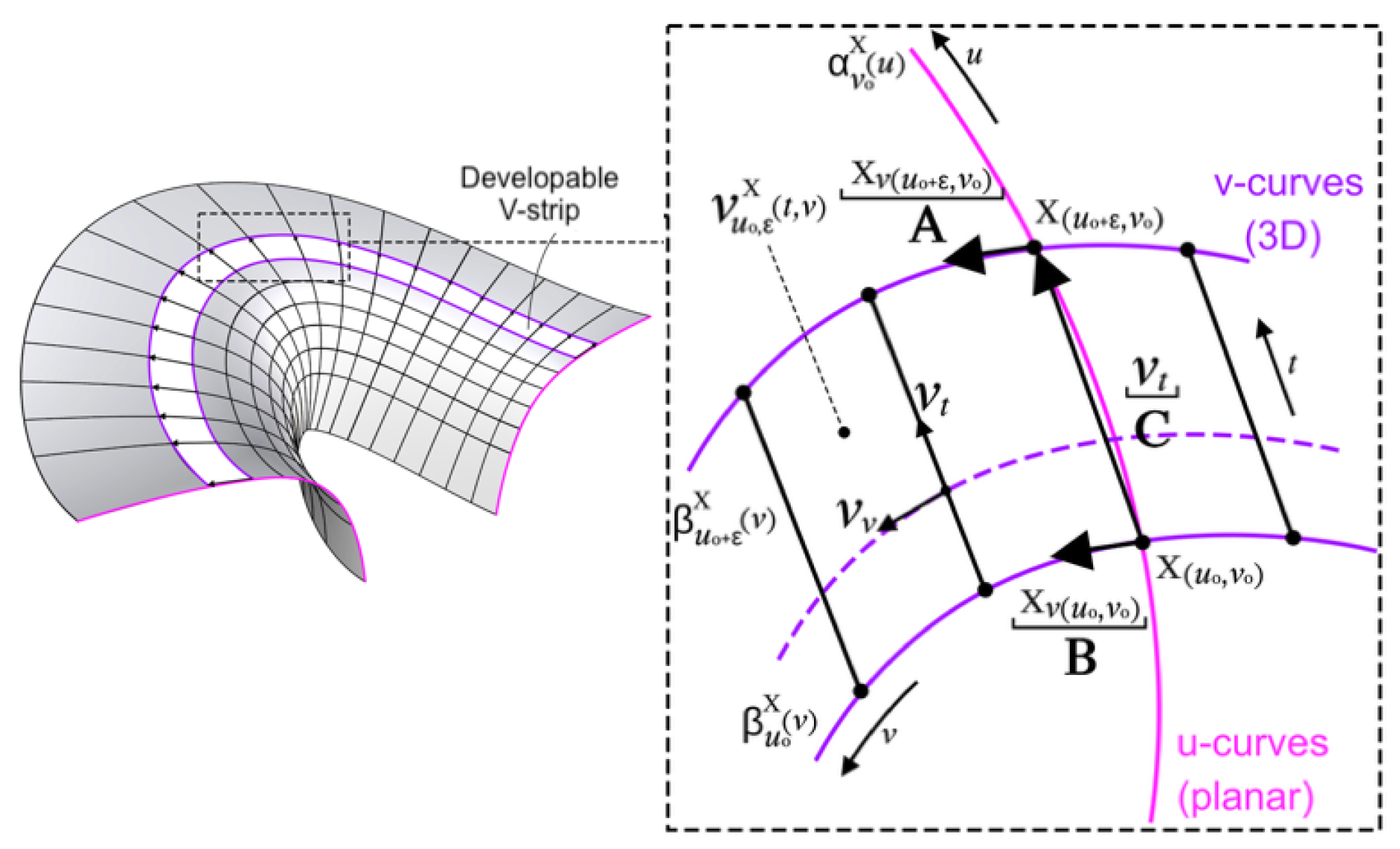
Figure 3.
Translation-type (level 1).
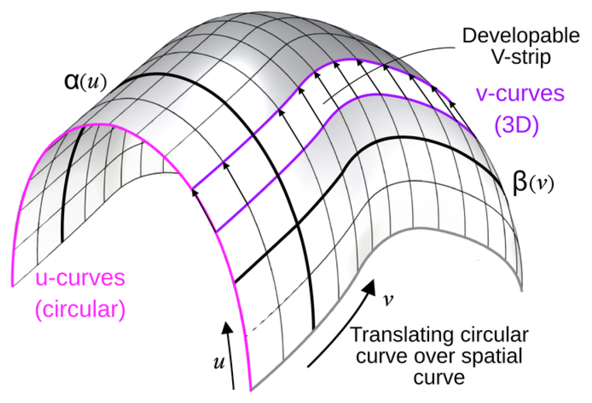
Figure 4.
Revolution-type (level 2).
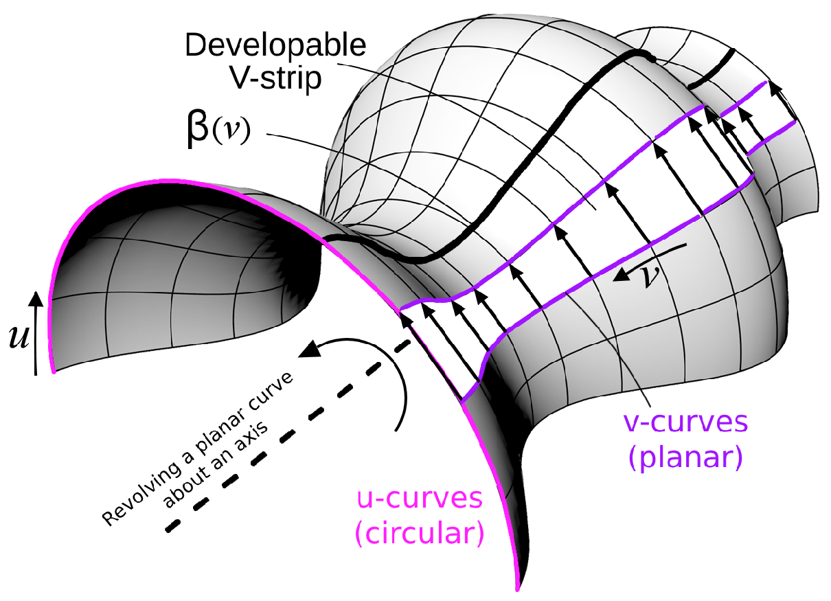
Figure 5.
Parabolic Cyclide-type (level 2).
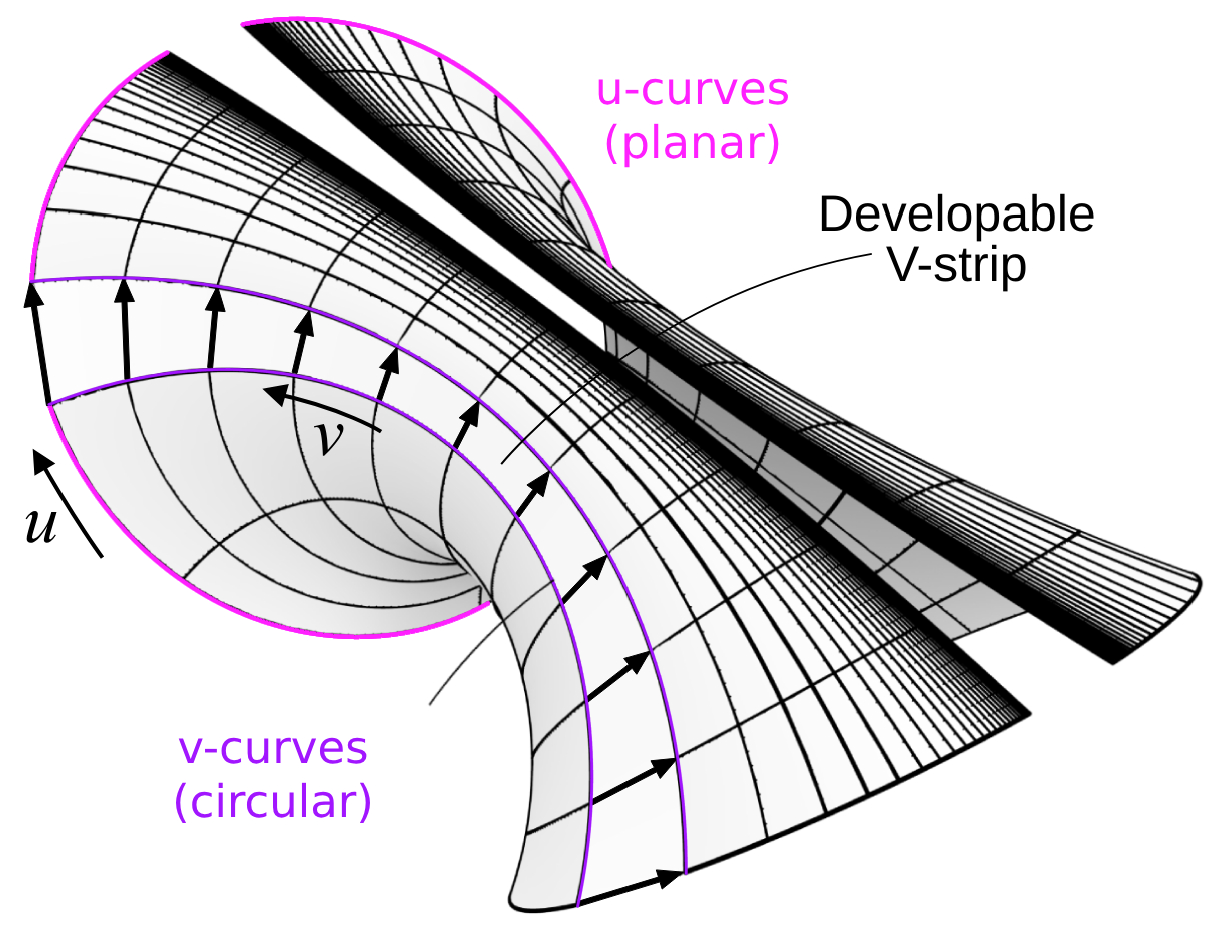
Figure 6.
Monge-type (level 2).

Figure 7.
Joachimsthal-type (level 2).
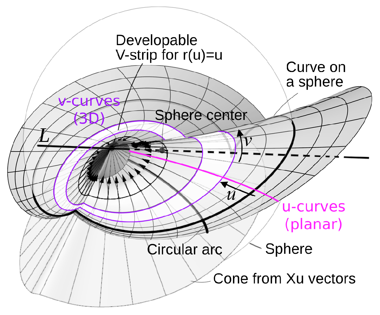
Figure 8.
Pencil-type (level 2).
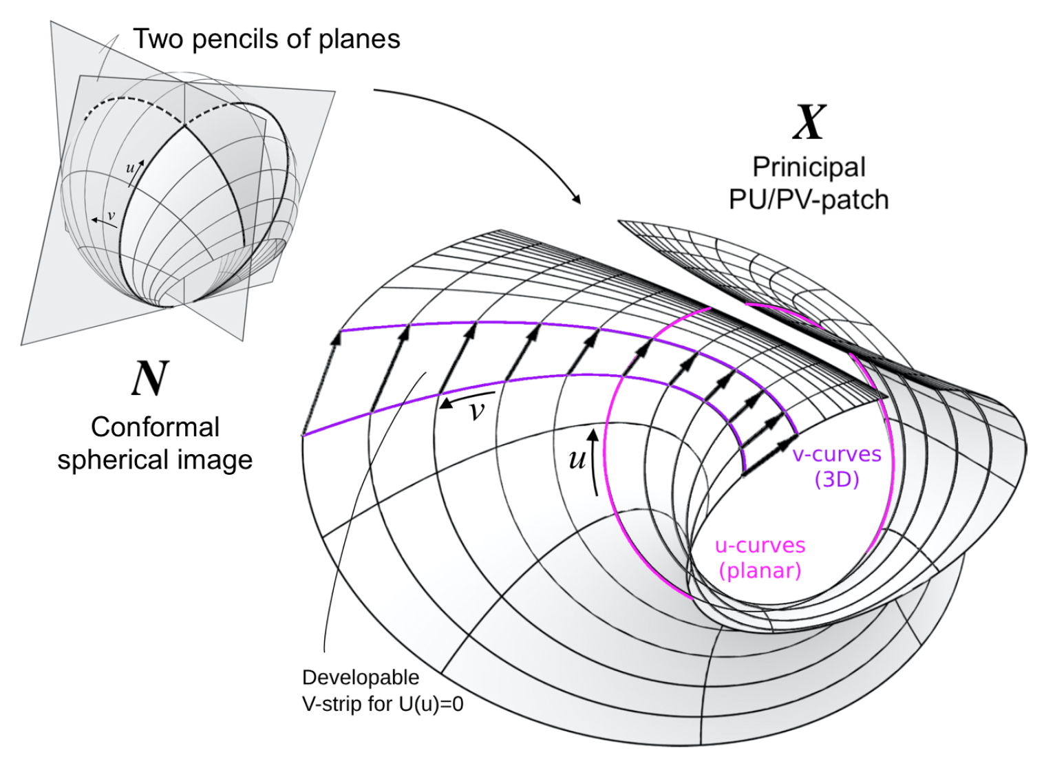
Figure 9.
Four nCGC-types (level 3).
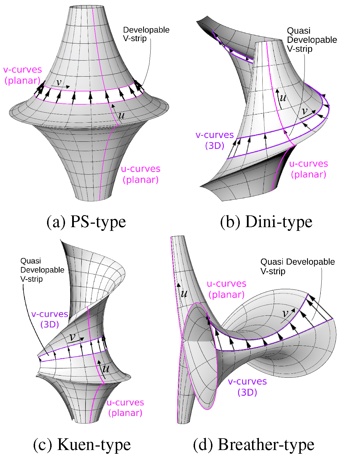
Figure 10.
Projective transform (level 1).
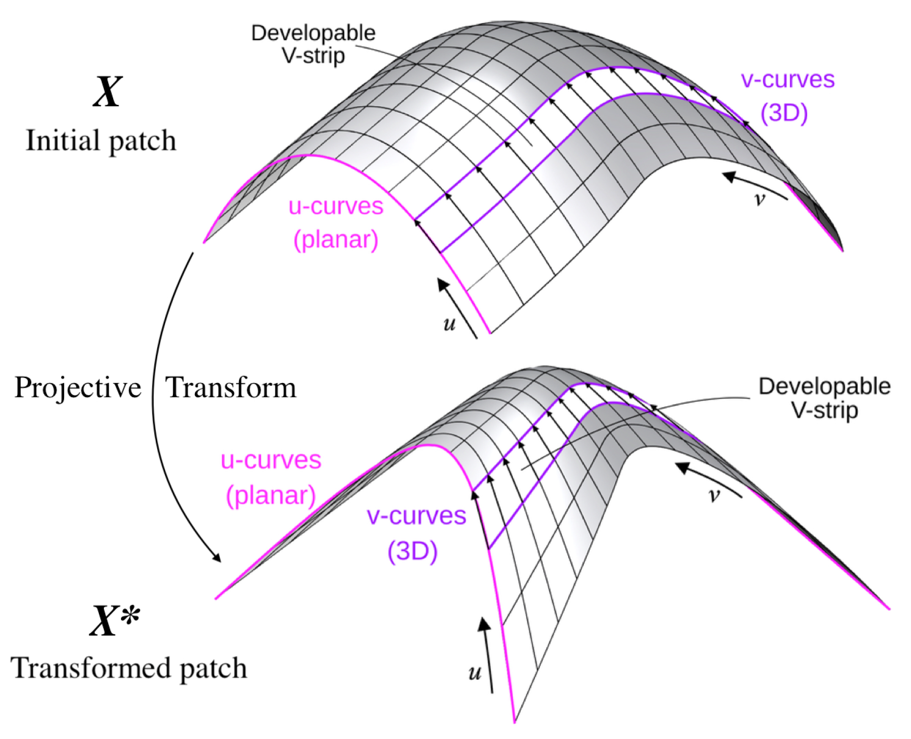
Figure 11.
Möbius transform (level 2).
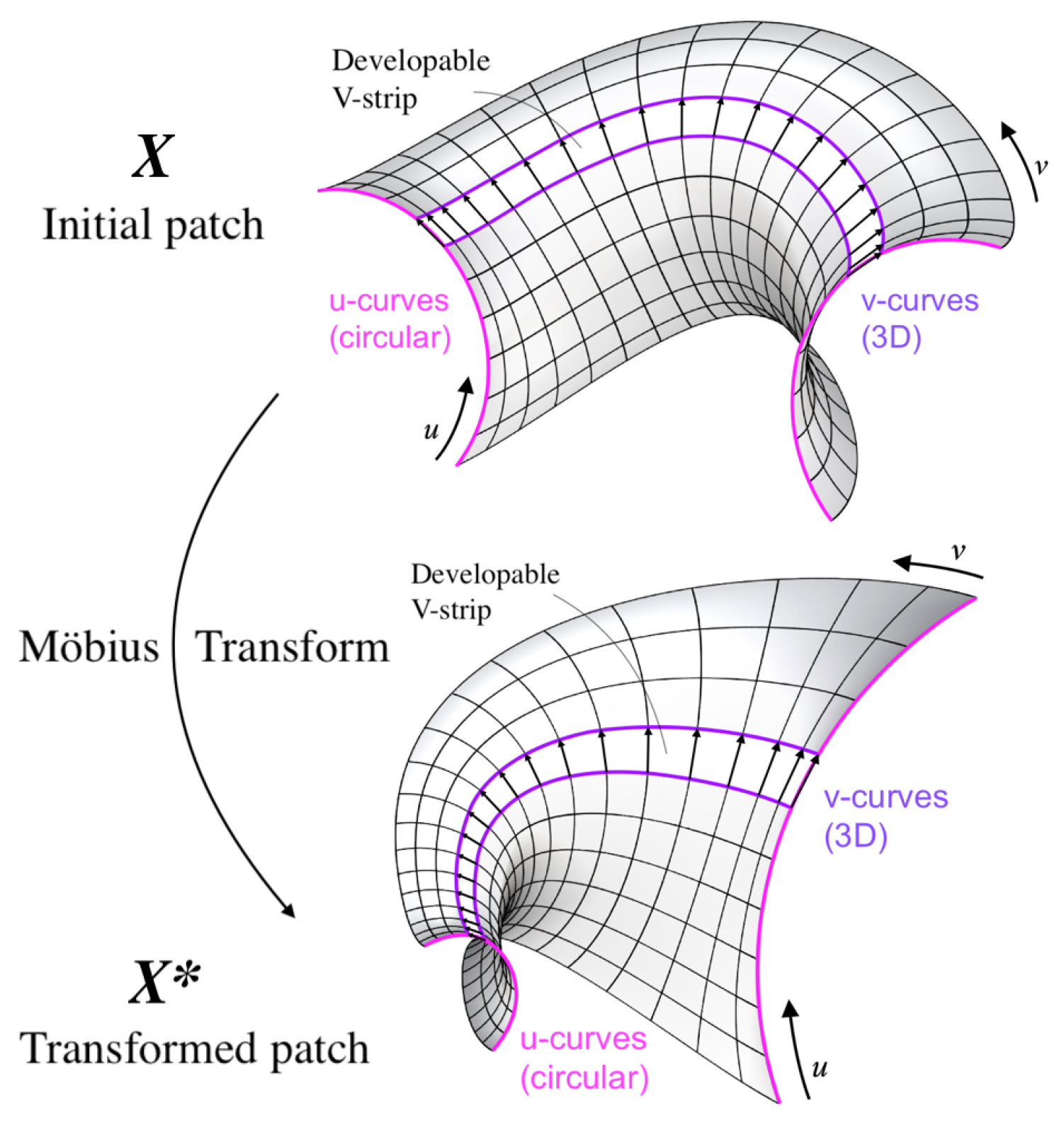
Figure 12.
Bäcklund transfrom (Geometric view).
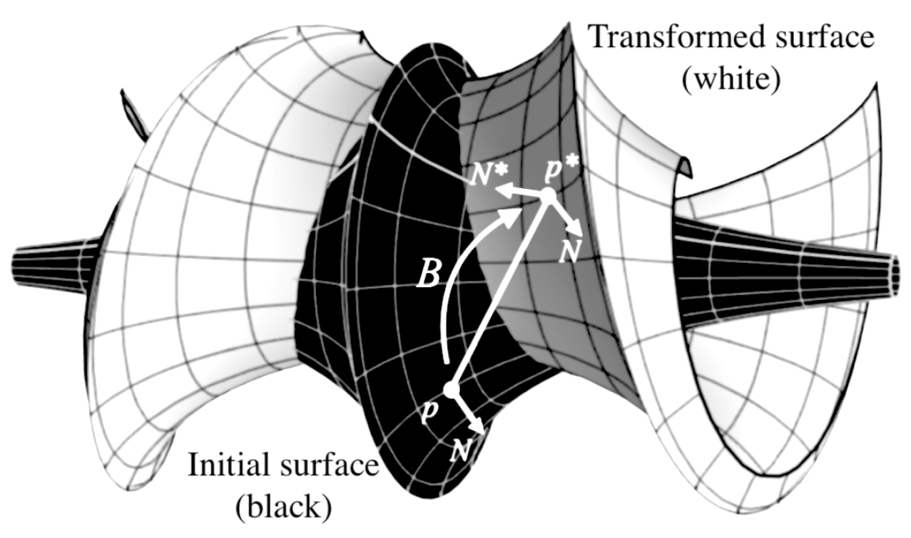
Figure 13.
Dini-type to Breather-type (level 3).
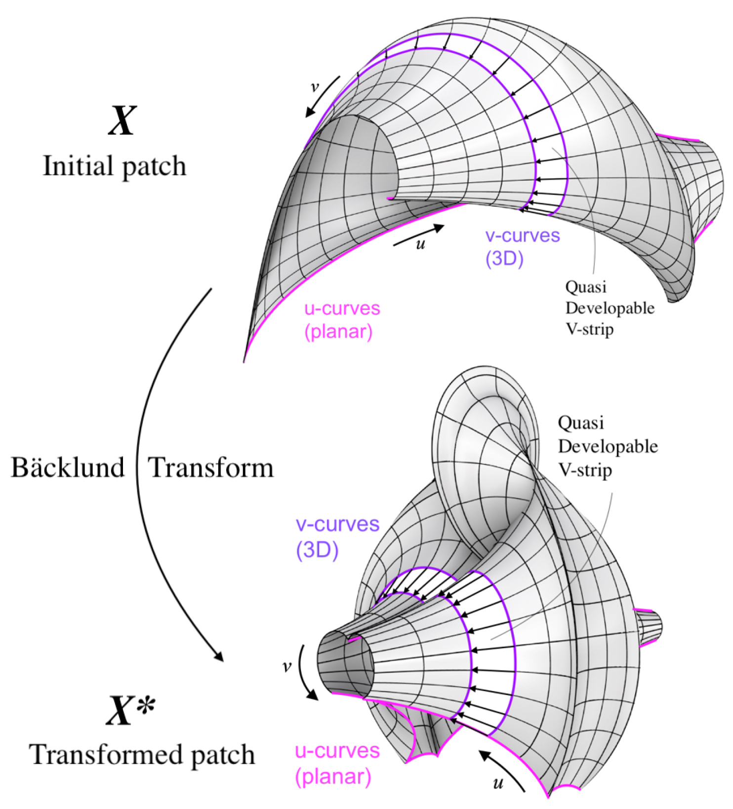
Figure 14.
Möbius transform of R-TOS CU-patch.
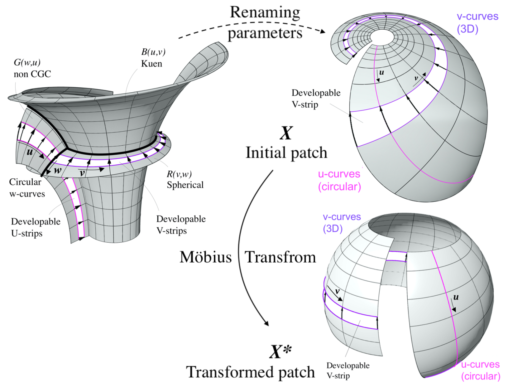
Figure 15.
Transforms corresponding levels.
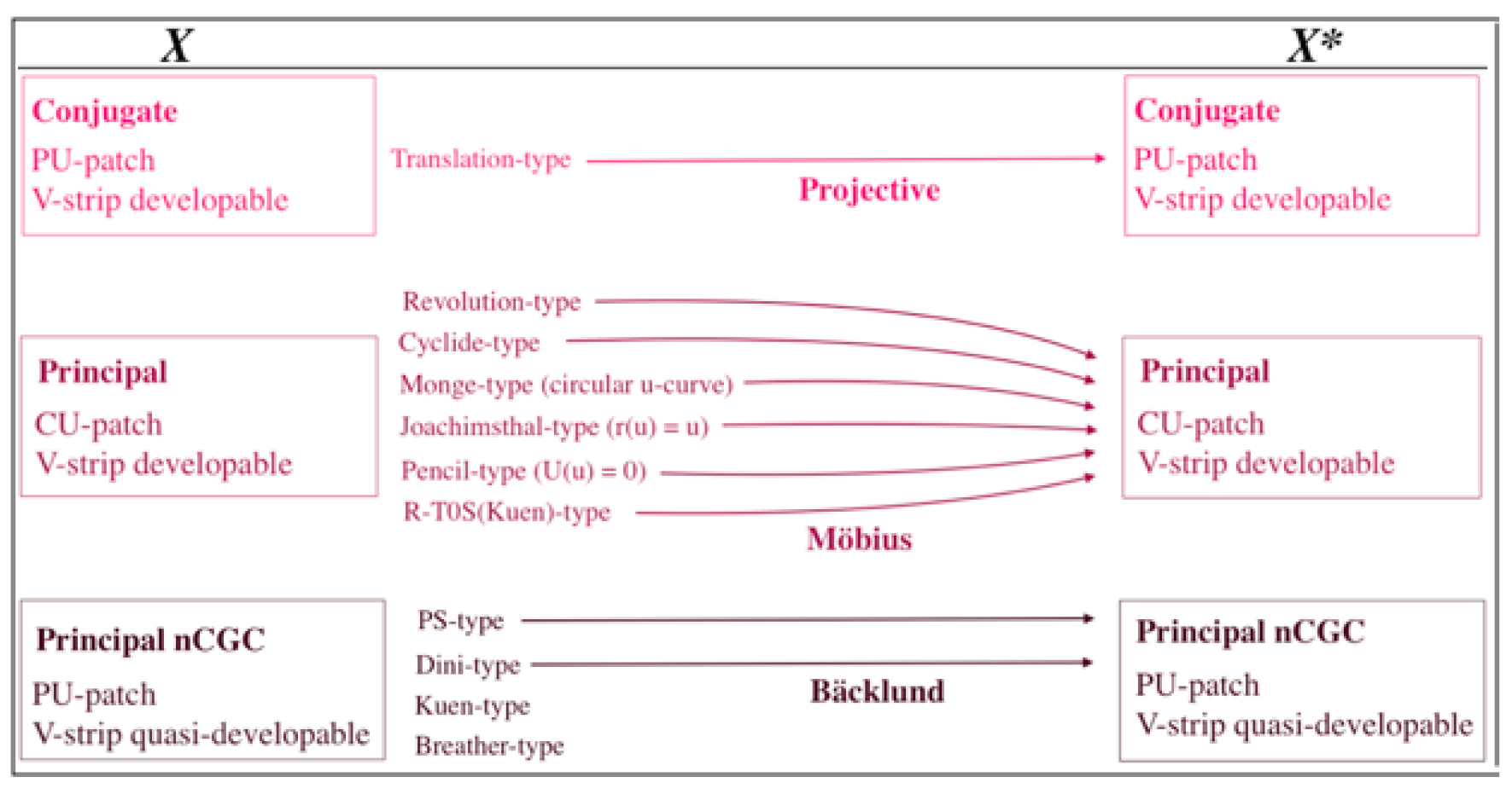
Figure 16.
Transforms non-corresponding levels.
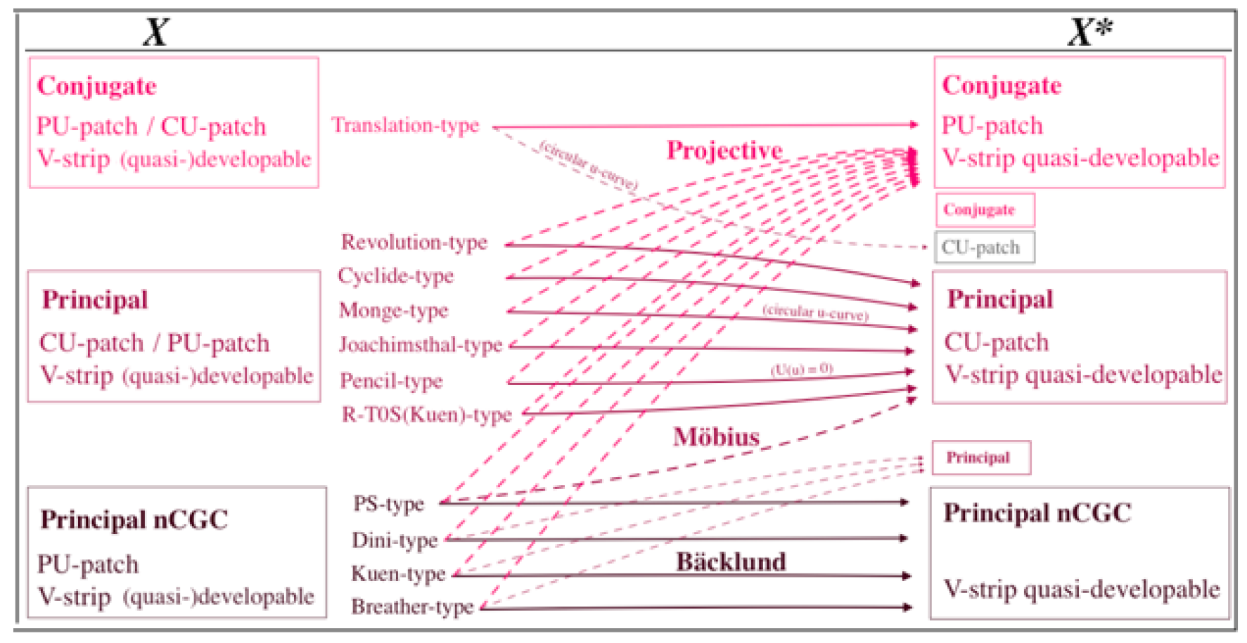
Figure 17.
Possible-paths diagram with ID-codes.
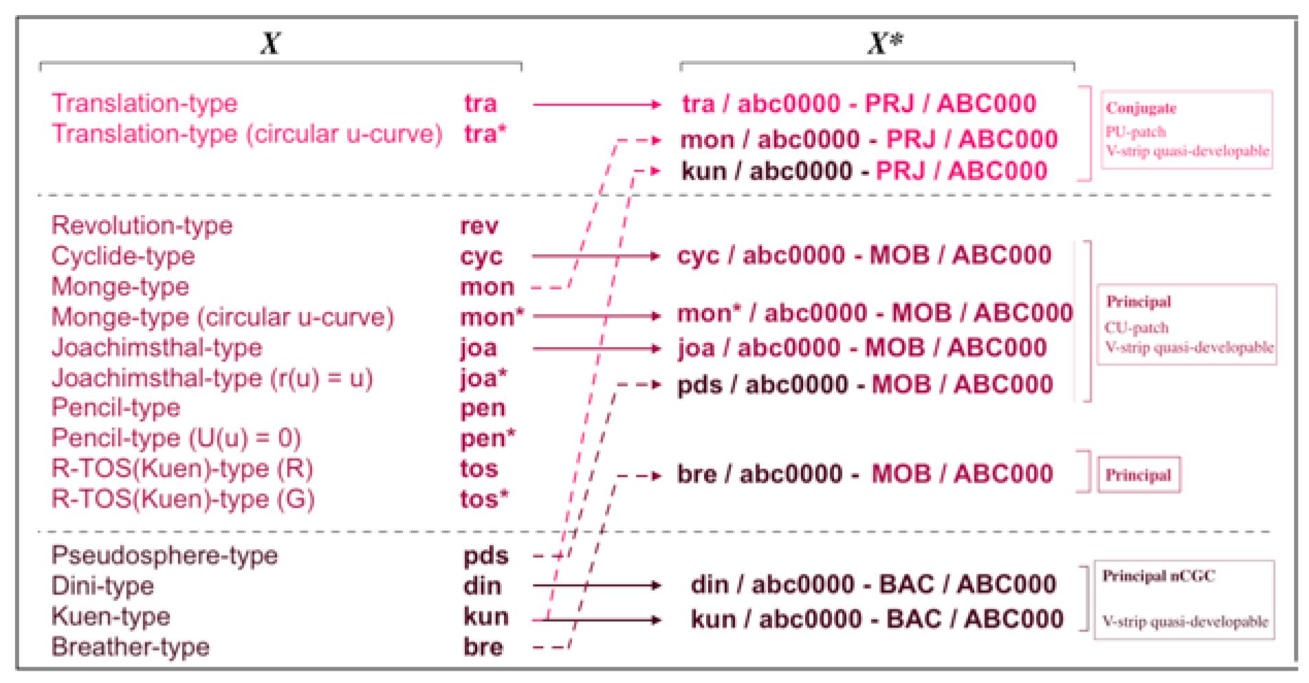
Figure 18.
Varying the patch-parameters l and f.
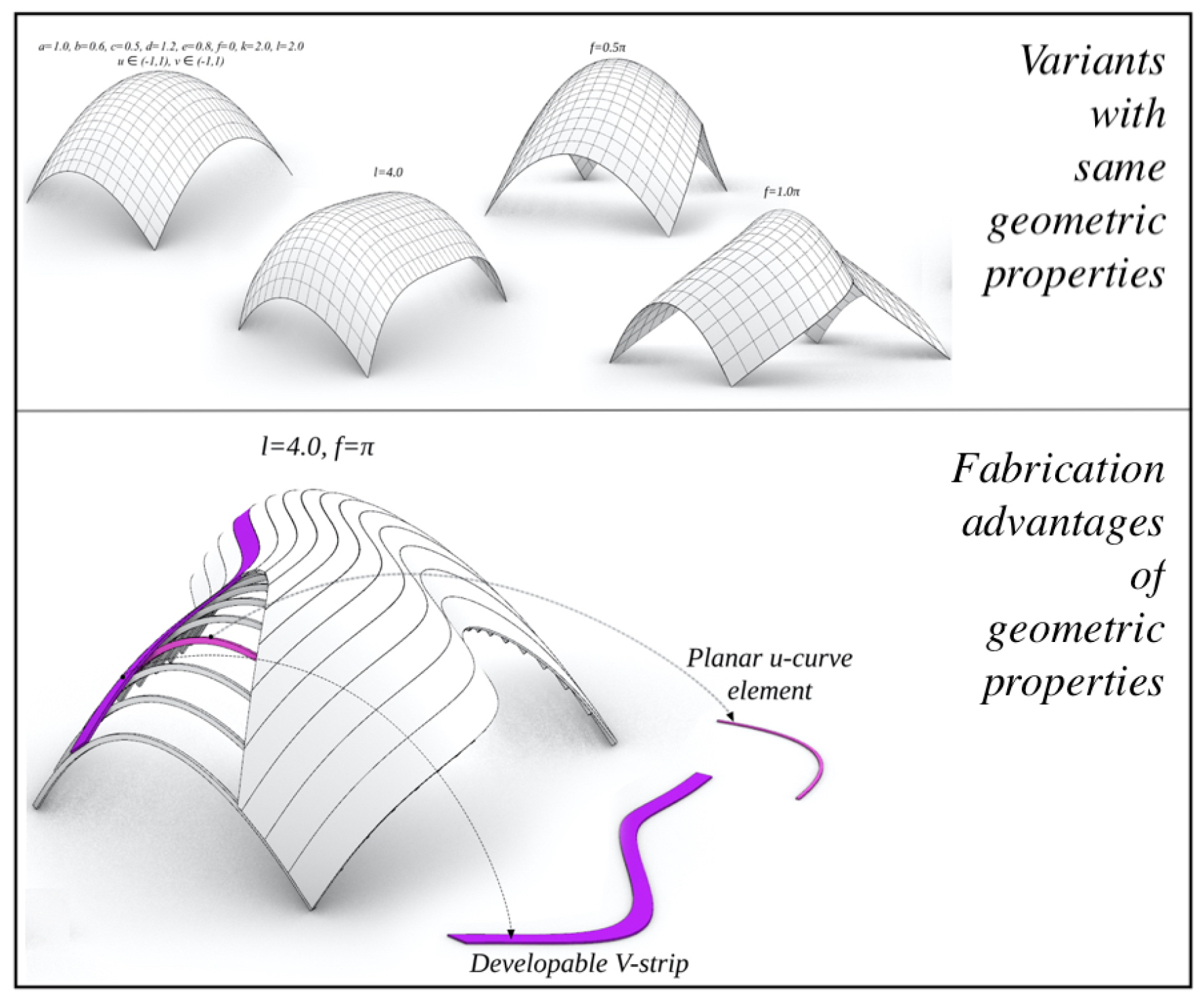
Figure 19.
Varying the patch-parameters o and k.
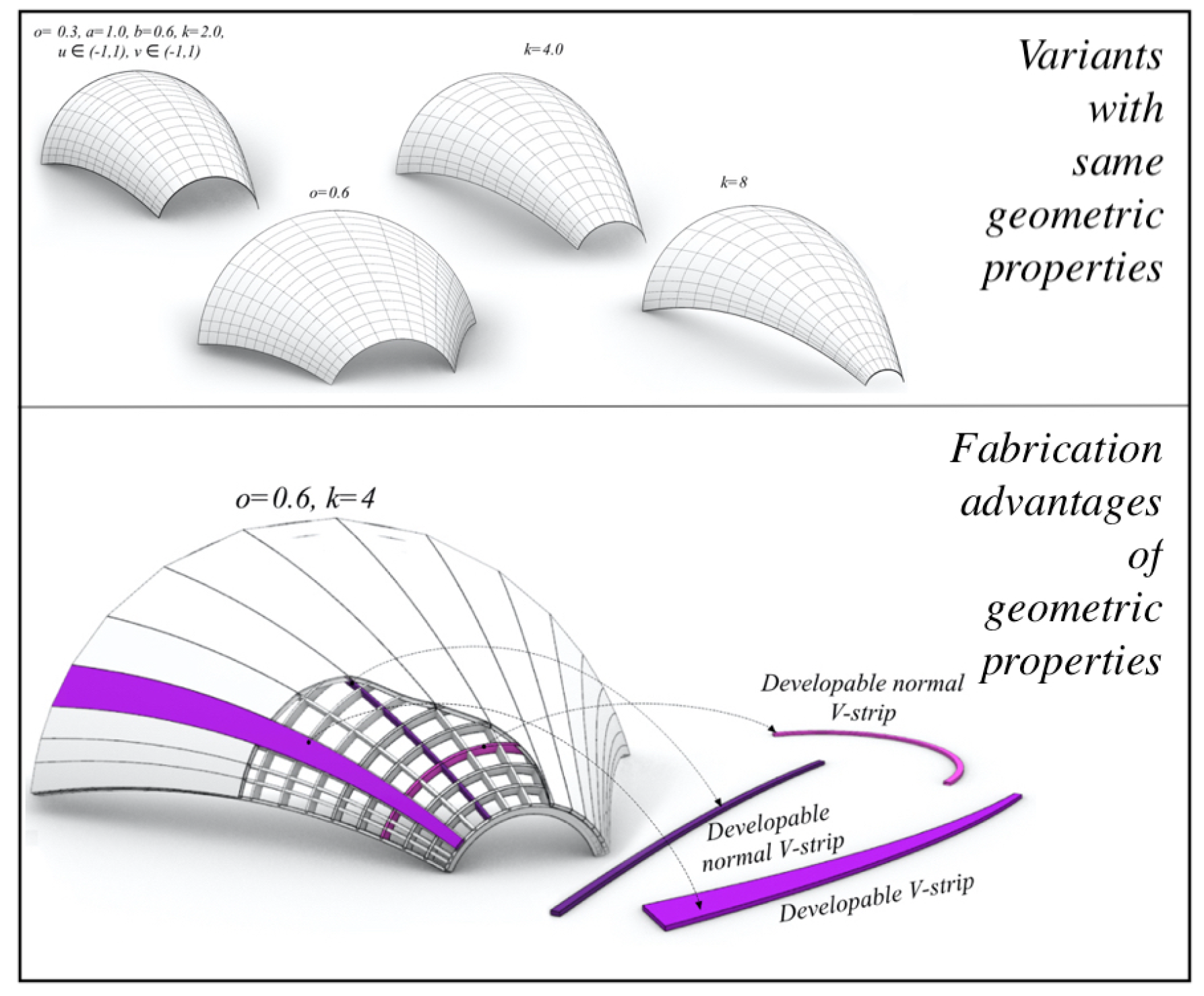
Figure 20.
Varying the patch-parameters s and w.
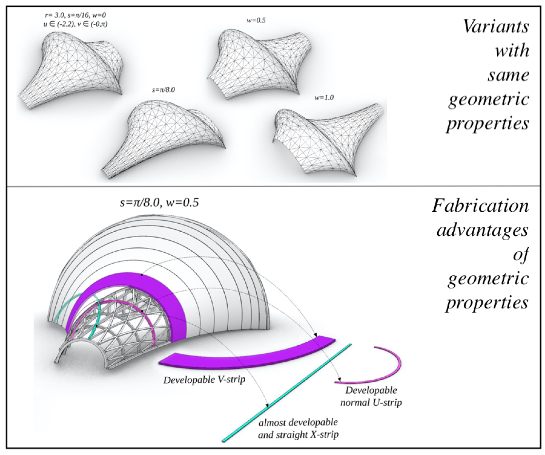
Figure 21.
Varying the transform-parameters .
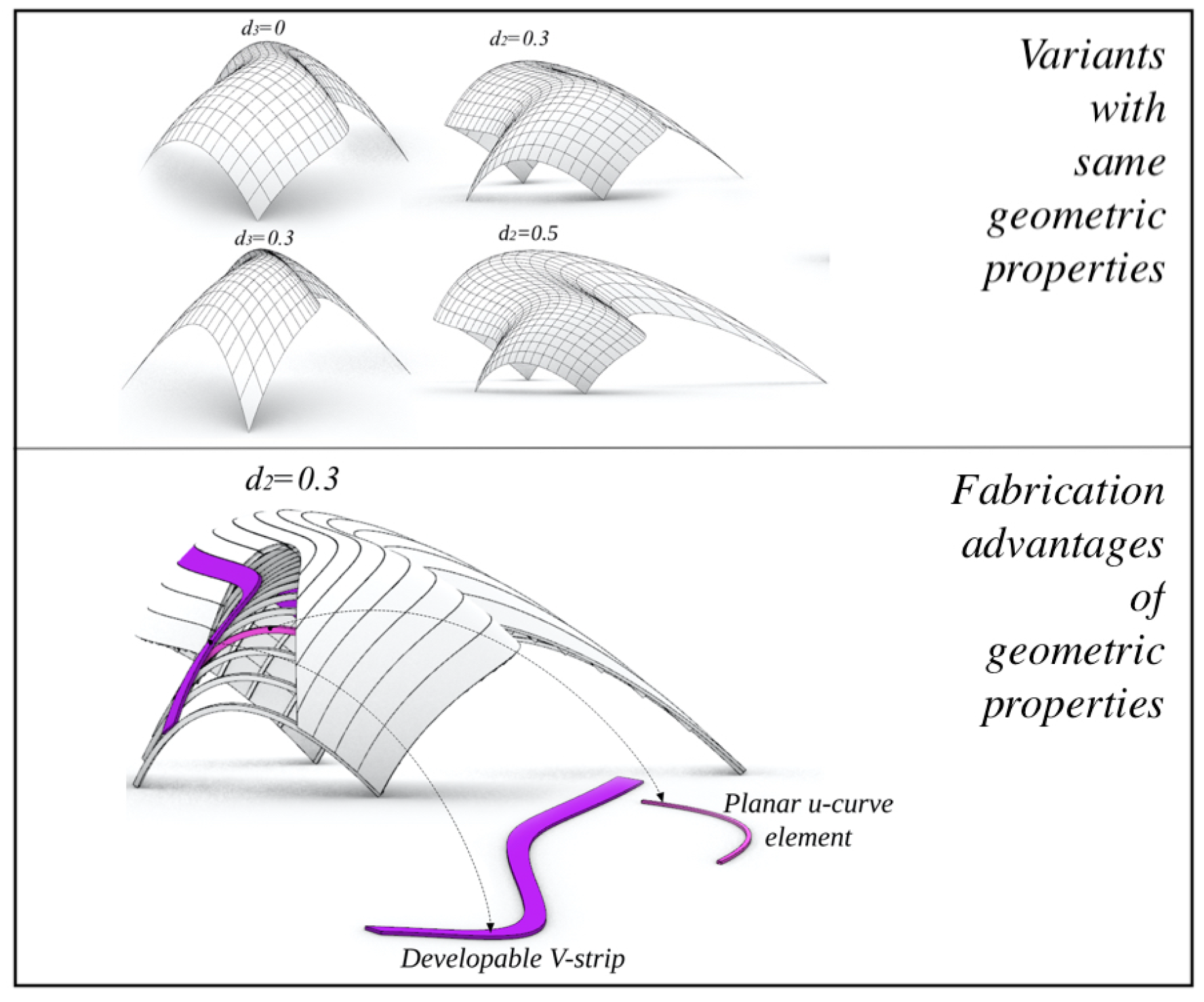
Figure 22.
Varying transform-parameters .
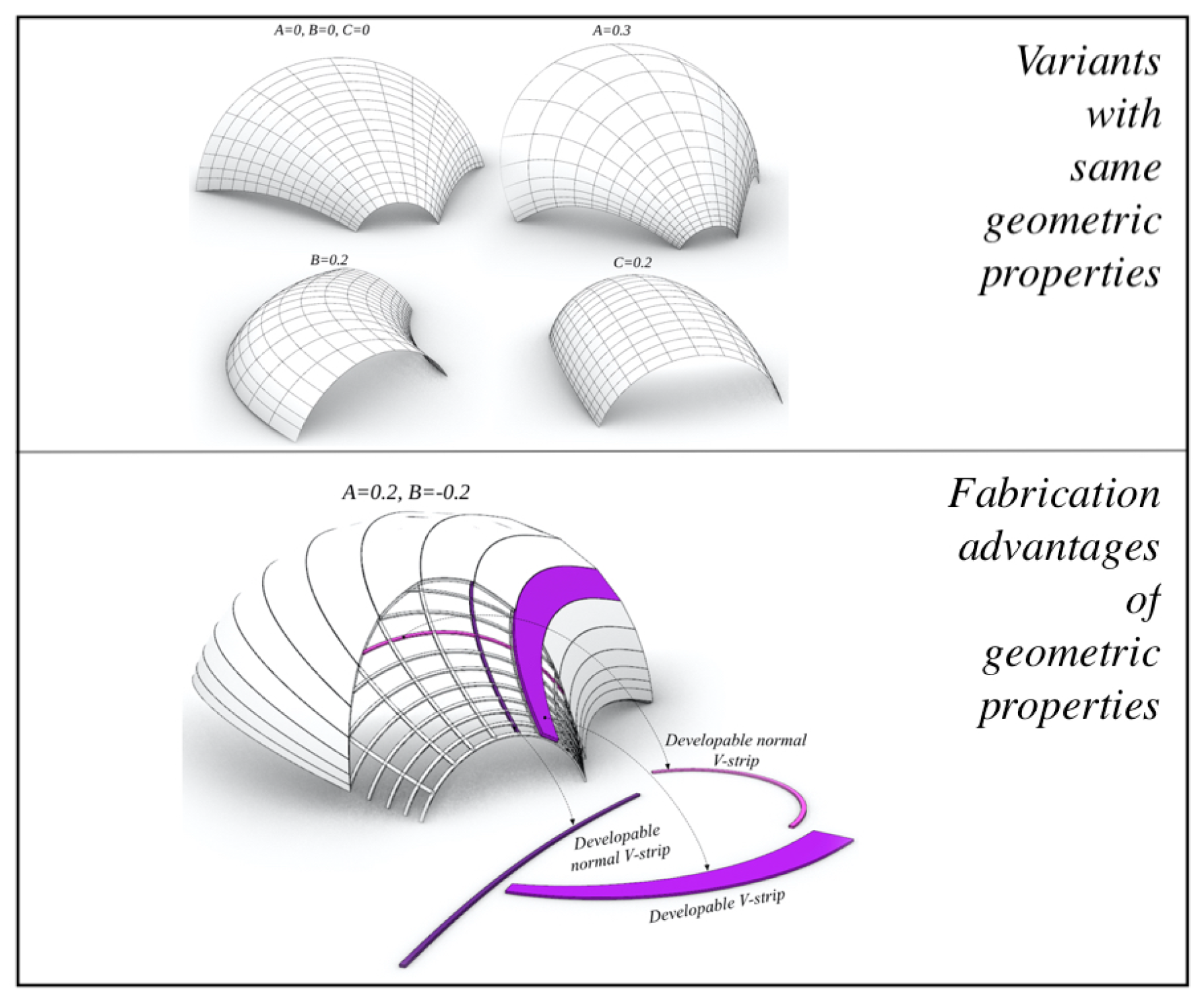
Figure 23.
Varying the transform-parameter D.
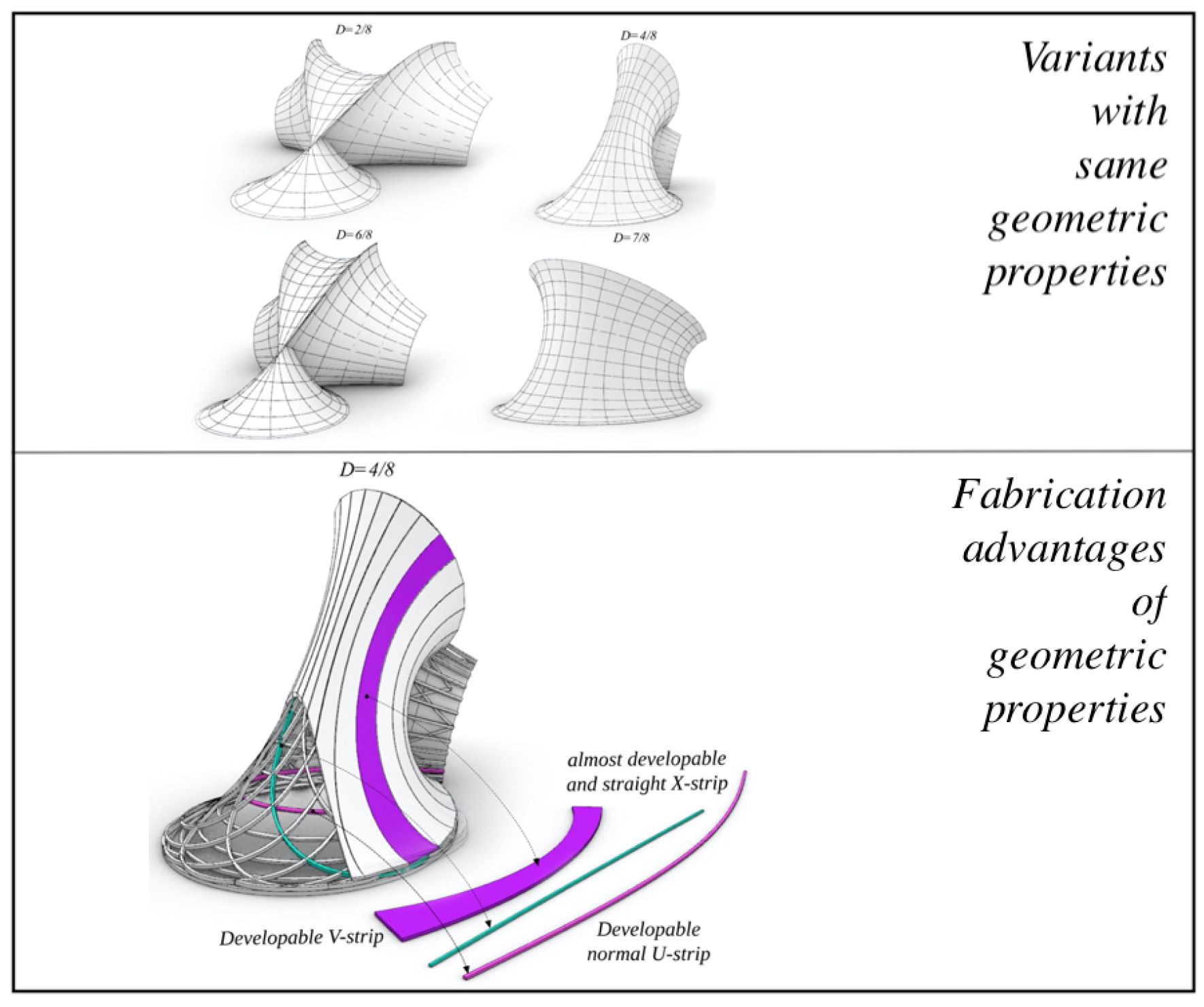
Figure 24.
Corresponding principal-asymptotic nets.
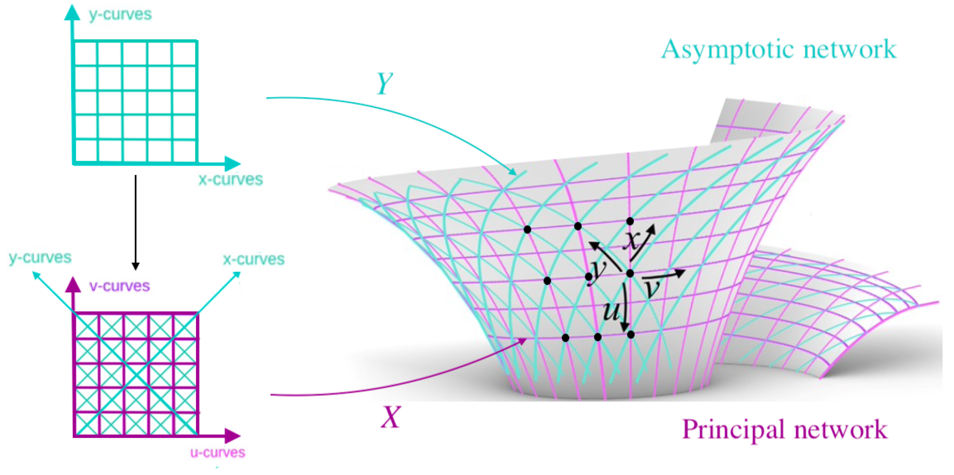
Figure 25.
Bring out the floral appearance.
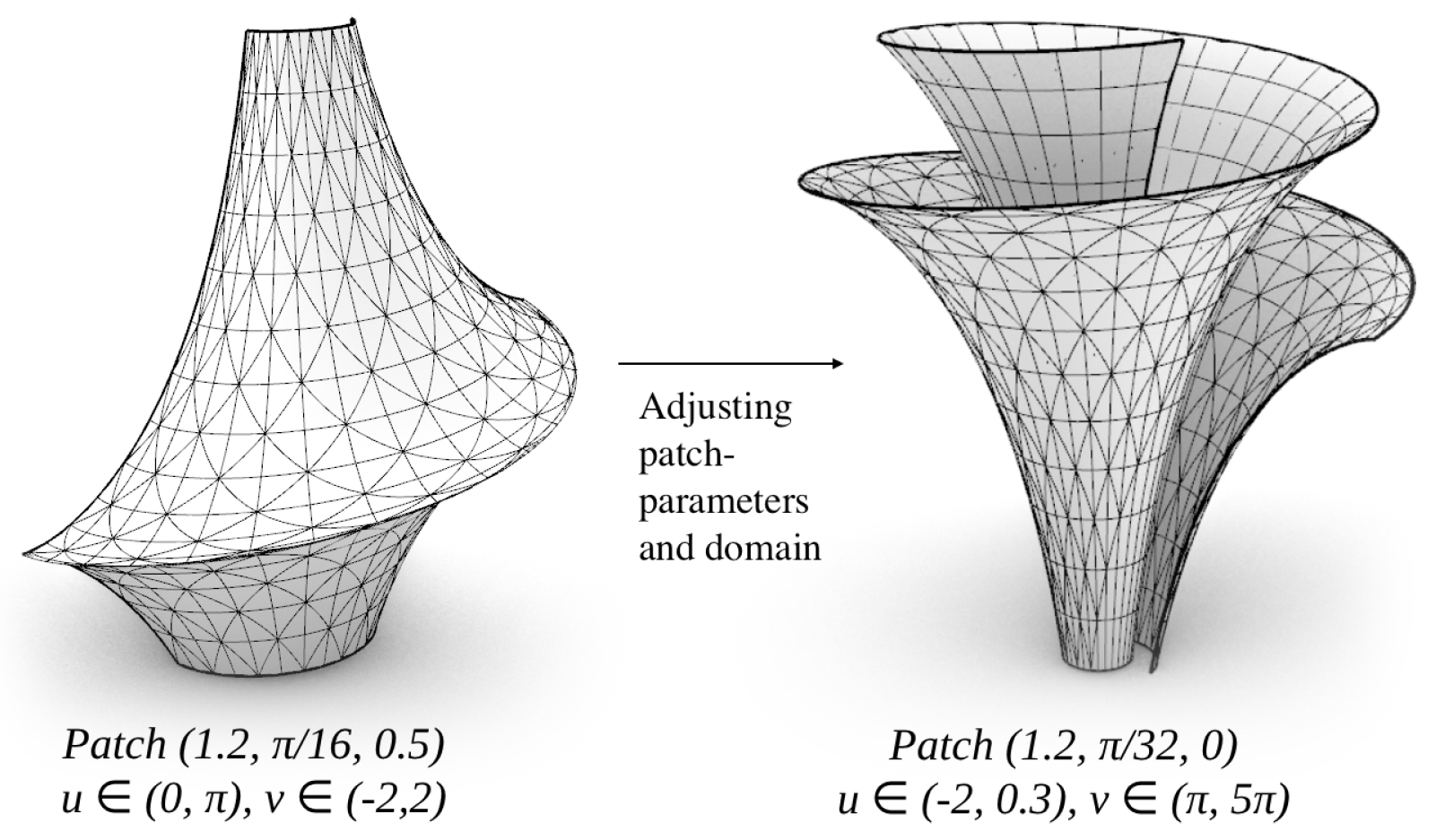
Figure 26.
Projective and Möbius transforms of Dini.
Disclaimer/Publisher’s Note: The statements, opinions and data contained in all publications are solely those of the individual author(s) and contributor(s) and not of MDPI and/or the editor(s). MDPI and/or the editor(s) disclaim responsibility for any injury to people or property resulting from any ideas, methods, instructions or products referred to in the content. |
© 2025 by the authors. Licensee MDPI, Basel, Switzerland. This article is an open access article distributed under the terms and conditions of the Creative Commons Attribution (CC BY) license (http://creativecommons.org/licenses/by/4.0/).
Copyright: This open access article is published under a Creative Commons CC BY 4.0 license, which permit the free download, distribution, and reuse, provided that the author and preprint are cited in any reuse.


