Deriving the Pontecorvo–Maki–Nakagawa–Sakata Matrix from Koide’s Mass Formula and Brannen’s Neutrino Mass Hypothesis: Resolving the Mystery of the θ₁₃ Rotation

1. Introduction

1.1. Koide’s Mass Formula

In 1982, Yoshio Koide first proposed the Koide mass formula [1,2] based on the study by Harari, Haut, and Weyers [3]:

${\displaystyle \frac{m_e+m_{\mu }+m_{\tau }}{(\sqrt{m_e}+\sqrt{m_{\mu }}+\sqrt{m_{\tau }}{)}^2}}={\displaystyle \frac{2}{3}}$,

which elegantly describes the relationship among the masses of the three generations of charged leptons.

1.2. Interpretation by Carl A. Brannen

In 2006, Carl A. Brannen provided an interpretation of the Koide mass formula in his paper [4]. Let the masses of e⁻, μ⁻, and τ⁻ be denoted as m₁, m₂, and m₃, respectively. The masses are experimentally determined as follows [5]:

m₁ = 0.51099 [MeV],

m₂ = 105.658367 [MeV],

m₃ = 1776.84 [MeV].

According to Brannen, the square root of each mass is expressed as:

$\sqrt{m_n}=17.715992(1+\sqrt{2}\mathrm{c}\mathrm{o}\mathrm{s}(0.222222+{\displaystyle \frac{2}{3}}n\pi ))[{\mathrm{M}\mathrm{e}\mathrm{V}}^{{\displaystyle \frac{1}{2}}}]$ for n = 1, 2, 3.

Using this formula, the following relationships hold:

$\sqrt{m_1}+\sqrt{m_2}+\sqrt{m_3}=17.715992\times 3[{\mathrm{M}\mathrm{e}\mathrm{V}}^{{\displaystyle \frac{1}{2}}}]$,

and $m_1+m_2+m_3={17.715992}^2\times (3+3)[\mathrm{M}\mathrm{e}\mathrm{V}]$.

Thus,

${\displaystyle \frac{m_1+m_2+m_3}{(\sqrt{m_1}+\sqrt{m_2}+\sqrt{m_3}{)}^2}}={\displaystyle \frac{{17.715992}^2\times 3\times 2}{{17.715992}^2\times 3^2}}={\displaystyle \frac{2}{3}}$.

This provides a deeper mathematical insight into the Koide mass formula.

1.3. Brannen’s Neutrino Mass Hypothesis

Brannen hypothesized that a similar relationship holds for neutrinos:

${\displaystyle \frac{m_1+m_2+m_3}{(-\sqrt{m_1}+\sqrt{m_2}+\sqrt{m_3}{)}^2}}={\displaystyle \frac{2}{3}}$.

Let the masses of v₁, v₂, and v₃, be denoted as m₁, m₂, and m₃, respectively. Brannen proposed the following expressions [4]:

$-\sqrt{m_n}={\displaystyle \frac{17715.992}{3^{11}}}(1+\sqrt{2}cos(0.222222+{\displaystyle \frac{1}{12}}\pi +{\displaystyle \frac{2}{3}}n\pi ))[{\mathrm{e}\mathrm{V}}^{{\displaystyle \frac{1}{2}}}]$ for n = 1,

the minus sign appears because the expression evaluates to a negative value when n = 1.

$\sqrt{m_n}={\displaystyle \frac{17715.992}{3^{11}}}(1+\sqrt{2}cos(0.222222+{\displaystyle \frac{1}{12}}\pi +{\displaystyle \frac{2}{3}}n\pi ))[{\mathrm{e}\mathrm{V}}^{{\displaystyle \frac{1}{2}}}]$ for n = 2, 3.

From these, the neutrino masses are calculated as:

m₁ = 0.383462 [MeV],

m₂ = 8.913487 [MeV],

m₃ = 50.711804 [MeV].

1.4. Constructing Two Three-Dimensional Mass Models

Here, a question arises: while Brannen indicates that the square root of the mass of v₁ is negative, what does it mean for the square root of a mass to be negative?

Could it imply that v₁ is antimatter, or might it suggest that v₁ travels faster than the speed of light, effectively moving backward in time? The observed v₁ should correspond to the positive square root of the mass.

Assuming Brannen’s hypothesis is valid, I propose that $-\sqrt{m_1}$ might be the origin of the ${\theta }_{13}$ rotation in the Pontecorvo-Maki-Nakagawa-Sakata (PMNS) matrix [6]. Based on Brannen’s hypothesis, I construct two three-dimensional mass models for neutrinos.

2. Method

2.1. Construction of the Neutrino Three-Dimensional Mass Models

Let the masses of ${\nu }_1$, ${\nu }_2$, and ${\nu }_3$, be denoted as $m_1$, $m_2$, and $m_3$, respectively, satisfying:

$m_1+m_2+m_3=60.008753[\mathrm{m}\mathrm{e}\mathrm{V}]={7.746532}^2[\mathrm{m}\mathrm{e}\mathrm{V}]$.

In three-dimensional space, let the origin be $\mathrm{O}$.

Define the radius:

$r=7.746532[{\mathrm{m}\mathrm{e}\mathrm{V}}^{{\displaystyle \frac{1}{2}}}]$,

where $\mathit{r}$ represents the radius of the sphere described by $x^2+y^2+z^2=r^2$.

Define the points:

$P_{-}(-\sqrt{m_1},\sqrt{m_2},\sqrt{m_3})$,

$P_{+}(\sqrt{m_1},\sqrt{m_2},\sqrt{m_3})$,

where both ${\mathrm{P}}_{-}$ and ${\mathrm{P}}_{+}$ lie on the sphere.

Additionally, define three points on the sphere:

$N_1(r,\mathrm{0,0})$,

$N_2(0,r,0)$,

$N_3(\mathrm{0,0},r)$.

The models are constructed in two patterns, based on the square roots of the neutrino masses:

1. The combination $-\sqrt{m_1},\sqrt{m_2},\sqrt{m_3}$,

2. The combination $\sqrt{m_1},\sqrt{m_2},\sqrt{m_3}$.

2.1.1. Case of the Combination

2.1.1.1. Vectors and Dot Products

Define the unit vector (I refer to this vector as the $\sqrt{m}$ unit vector):

$\overrightarrow{{\mathrm{O}\mathrm{M}}_{-}}={\displaystyle \frac{\overrightarrow{{\mathrm{O}\mathrm{P}}_{-}}}{\Vert \overrightarrow{{\mathrm{O}\mathrm{P}}_{-}}\Vert }}$.

Define the following vectors originating from $\mathrm{O}$:

${\mathit{M}}_{-}=\overrightarrow{{\mathrm{O}\mathrm{M}}_{-}}=(-\mathrm{0.079938,0.385404,0.919279})$,

${\mathit{N}}_{1-}=\overrightarrow{{\mathrm{O}\mathrm{N}}_1}=(r,\mathrm{0,0})$,

${\mathit{N}}_{2-}=\overrightarrow{{\mathrm{O}\mathrm{N}}_2}=(0,r,0)$,

${\mathit{N}}_{3-}=\overrightarrow{{\mathrm{O}\mathrm{N}}_3}=(\mathrm{0,0},r)$.

The dot products are calculated as follows:

${\mathit{N}}_{1-}·{\mathit{M}}_{-}=-0.079938r=-0.61924[{\mathrm{m}\mathrm{e}\mathrm{V}}^{{\displaystyle \frac{1}{2}}}]=-\sqrt{m_1}$,

${\mathit{N}}_{2-}·{\mathit{M}}_{-}=0.385404r=2.985546[{\mathrm{m}\mathrm{e}\mathrm{V}}^{{\displaystyle \frac{1}{2}}}]=\sqrt{m_2}$,

${\mathit{N}}_{3-}·{\mathit{M}}_{-}=0.919279r=7.121222[{\mathrm{m}\mathrm{e}\mathrm{V}}^{{\displaystyle \frac{1}{2}}}]=\sqrt{m_3}$.

To align the direction of ${\mathit{M}}_{-}$ with the $\mathit{x}$-axis, ${\mathit{M}}_{-}$, ${\mathit{N}}_{1-}$, ${\mathit{N}}_{2-}$, and ${\mathit{N}}_{3-}$ are rotated around the origin in three-dimensional space.

2.1.1.2. Initial Coordinates

The initial coordinates are expressed as:

$\left[\begin{array}{c}{\mathit{M}}_{-}\\ {\mathit{N}}_{1-}\\ {\mathit{N}}_{2-}\\ {\mathit{N}}_{3-}\end{array}\right]=\left[\begin{array}{ccc}-0.079938& 0.385404& 0.919279\\ r& 0& 0\\ 0& r& 0\\ 0& 0& r\end{array}\right]\left[\begin{array}{c}x\\ y\\ z\end{array}\right]$.

2.1.1.3. Rotation in the $xy$-Plane

Using $\cos {\alpha }_{-}=-0.203091$ and $\sin {\alpha }_{-}=-0.979160$, corresponding to ${\alpha }_{-}\approx -1.775310\left[\mathrm{r}\mathrm{a}\mathrm{d}\right]$, a rotation in the $xy$-plane is applied:

$\left[\begin{array}{c}{\mathit{M}}_{-}\\ {\mathit{N}}_{1-}\\ {\mathit{N}}_{2-}\\ {\mathit{N}}_{3-}\end{array}\right]=\left[\begin{array}{ccc}0.393607& 0& 0.919279\\ -0.203091r& -0.979160r& 0\\ 0.979160r& -0.203091r& 0\\ 0& 0& r\end{array}\right]\left[\begin{array}{c}x\\ y\\ z\end{array}\right]$.

2.1.1.4. Rotation in the $\mathit{x}\mathit{z}$-Plane

Using $\cos {\beta }_{-}=0.393607$ and $\sin {\beta }_{-}=-0.919279$, corresponding to ${\beta }_{-}\approx -1.166244\left[\mathrm{r}\mathrm{a}\mathrm{d}\right]$, a rotation in the $xz$-plane is applied:

$\left[\begin{array}{c}{\mathit{M}}_{-}\\ {\mathit{N}}_{1-}\\ {\mathit{N}}_{2-}\\ {\mathit{N}}_{3-}\end{array}\right]=\left[\begin{array}{ccc}1& 0& 0\\ -0.079938r& -0.979160r& 0.186697r\\ 0.385404r& -0.203091r& -0.900121r\\ 0.919279r& 0& 0.393607r\end{array}\right]\left[\begin{array}{c}x\\ y\\ z\end{array}\right]$.

2.1.1.5. Rotation in the $yz$-Plane

Using $\cos {\gamma }_{-}=0.220094$ and $\sin {\gamma }_{-}=-0.975479$, corresponding to ${\gamma }_{-}\approx -1.348886\left[\mathrm{r}\mathrm{a}\mathrm{d}\right]$, a rotation in the $yz$-plane is applied (optional for visualization purposes to set the $\mathcal{Z}$-component of to ${\mathit{N}}_{2-}$ to $\begin{array}{c}0\end{array}$ ):

$\left[\begin{array}{c}{\mathit{M}}_{-}\\ {\mathit{N}}_{1-}\\ {\mathit{N}}_{2-}\\ {\mathit{N}}_{3-}\end{array}\right]=\left[\begin{array}{ccc}1& 0& 0\\ -0.079938r& -0.033388r& 0.996241r\\ 0.385404r& -0.922748r& 0\\ 0.919279r& 0.383955r& 0.086631r\end{array}\right]\left[\begin{array}{c}x\\ y\\ z\end{array}\right]$.

The $\mathit{x}$-components of ${\mathit{N}}_{1-}$, ${\mathit{N}}_{2-}$ and ${\mathit{N}}_{3-}$ denote $-\sqrt{m_1}$, $\sqrt{m_2}$, and $\sqrt{m_3}$, respectively, thus associating each vector with the respective neutrino.

2.1.2. Case of the Combination $\sqrt{m_1},\sqrt{m_2},\sqrt{m_3}$

2.1.2.1. Vectors and Dot Products

Define the unit vector:

$\overrightarrow{{\mathrm{O}\mathrm{M}}_{+}}={\displaystyle \frac{\overrightarrow{{\mathrm{O}\mathrm{P}}_{+}}}{\Vert \overrightarrow{{\mathrm{O}\mathrm{P}}_{+}}\Vert }}$.

Define the following vectors originating from $\mathrm{O}$:

${\mathit{M}}_{+}=\overrightarrow{{\mathrm{O}\mathrm{M}}_{+}}=(\mathrm{0.079938,0.385404,0.919279})$,

${\mathit{N}}_{1+}=\overrightarrow{{\mathrm{O}\mathrm{N}}_1}=(r,\mathrm{0,0})$,

${\mathit{N}}_{2+}=\overrightarrow{{\mathrm{O}\mathrm{N}}_2}=(0,r,0)$,

${\mathit{N}}_{3+}=\overrightarrow{{\mathrm{O}\mathrm{N}}_3}=(\mathrm{0,0},r)$.

The dot products are calculated as follows:

${\mathit{N}}_{1+}·{\mathit{M}}_{+}=0.079938r=0.61924[{\mathrm{m}\mathrm{e}\mathrm{V}}^{{\displaystyle \frac{1}{2}}}]=\sqrt{m_1}$,

${\mathit{N}}_{2+}·{\mathit{M}}_{+}=0.385404r=2.985546[{\mathrm{m}\mathrm{e}\mathrm{V}}^{{\displaystyle \frac{1}{2}}}]=\sqrt{m_2}$,

${\mathit{N}}_{3+}·{\mathit{M}}_{+}=0.919279r=7.121222[{\mathrm{m}\mathrm{e}\mathrm{V}}^{{\displaystyle \frac{1}{2}}}]=\sqrt{m_3}$.

To align the direction of ${\mathit{M}}_{+}$ with the $\mathit{x}$-axis, ${\mathit{M}}_{+}$, ${\mathit{N}}_{1+}$, ${\mathit{N}}_{2+}$, and ${\mathit{N}}_{3+}$ are rotated around the origin in three-dimensional space.

2.1.2.2. Initial Coordinates

The initial coordinates are expressed as:

$\left[\begin{array}{c}{\mathit{M}}_{+}\\ {\mathit{N}}_{1+}\\ {\mathit{N}}_{2+}\\ {\mathit{N}}_{3+}\end{array}\right]=\left[\begin{array}{ccc}0.079938& 0.385404& 0.919279\\ r& 0& 0\\ 0& r& 0\\ 0& 0& r\end{array}\right]\left[\begin{array}{c}x\\ y\\ z\end{array}\right]$.

2.1.2.3. Rotation in the $xy$-Plane

Using $\cos {\alpha }_{+}=0.203091$ and $\sin {\alpha }_{+}=-0.979160$, corresponding to ${\alpha }_{+}\approx -1.366283\left[\mathrm{r}\mathrm{a}\mathrm{d}\right]$, a rotation in the $xy$-plane is applied:

$\left[\begin{array}{c}{\mathit{M}}_{+}\\ {\mathit{N}}_{1+}\\ {\mathit{N}}_{2+}\\ {\mathit{N}}_{3+}\end{array}\right]=\left[\begin{array}{ccc}0.393607& 0& 0.919279\\ 0.203091r& -0.979160r& 0\\ 0.979160r& 0.203091r& 0\\ 0& 0& r\end{array}\right]\left[\begin{array}{c}x\\ y\\ z\end{array}\right]$.

2.1.2.4. Rotation in the $\mathit{x}\mathit{z}$-Plane

Using $\cos {\beta }_{+}=0.393607$ and $\sin {\beta }_{+}=-0.919279$, corresponding to ${\beta }_{+}\approx -1.166244\left[\mathrm{r}\mathrm{a}\mathrm{d}\right]$, a rotation in the $\mathit{x}\mathit{z}$-plane is applied:

$\left[\begin{array}{c}{\mathit{M}}_{+}\\ {\mathit{N}}_{1+}\\ {\mathit{N}}_{2+}\\ {\mathit{N}}_{3+}\end{array}\right]=\left[\begin{array}{ccc}1& 0& 0\\ 0.079938r& -0.979160r& -0.186697r\\ 0.385404r& 0.203091r& -0.900121r\\ 0.919279r& 0& 0.393607r\end{array}\right]\left[\begin{array}{c}x\\ y\\ z\end{array}\right]$.

2.1.2.5. Rotation in the $yz$-Plane

Using $\cos {\gamma }_{+}=-0.220094$ and $\sin {\gamma }_{+}=-0.975479$, corresponding to ${\gamma }_{+}\approx -1.792707\left[\mathrm{r}\mathrm{a}\mathrm{d}\right]$, a rotation in the $yz$-plane is applied:

$\left[\begin{array}{c}{\mathit{M}}_{+}\\ {\mathit{N}}_{1+}\\ {\mathit{N}}_{2+}\\ {\mathit{N}}_{3+}\end{array}\right]=\left[\begin{array}{ccc}1& 0& 0\\ 0.079938r& 0.033388r& 0.996241r\\ 0.385404r& -0.922748r& 0\\ 0.919279r& 0.383955r& -0.086631r\end{array}\right]\left[\begin{array}{c}x\\ y\\ z\end{array}\right]$.

The $\mathit{x}$-components of ${\mathit{N}}_{1+}$ , ${\mathit{N}}_{2+}$ and ${\mathit{N}}_{3+}$ denote $\sqrt{m_1}$, $\sqrt{m_2}$, and $\sqrt{m_3}$, respectively, thus associating each vector with the respective neutrino.

3. Result

Figure 1 shows the results of the two neutrino three-dimensional mass models.

Figure 1. Two neutrino three-dimensional mass models.

Figure 1. Two neutrino three-dimensional mass models.

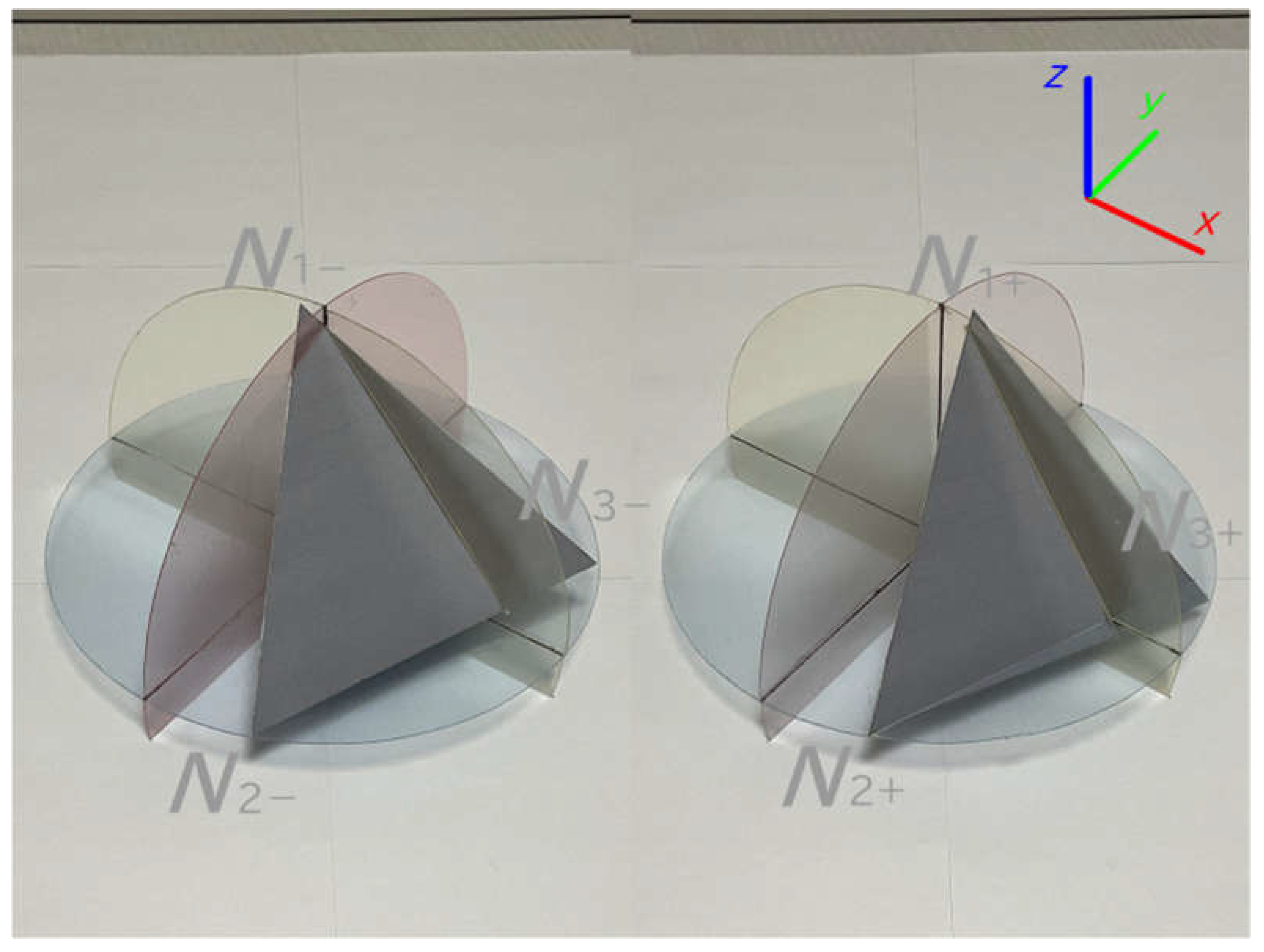
The relationship between the two models can be expressed as:

$\left[\begin{array}{c}{\mathit{N}}_{1-}\\ {\mathit{N}}_{2-}\\ {\mathit{N}}_{3-}\end{array}\right]=\left[\begin{array}{ccc}0.984990& 0.000000& -0.172610\\ 0.000000& 1.000000& 0.000000\\ 0.172610& 0.000000& 0.984990\end{array}\right]\left[\begin{array}{c}{\mathit{N}}_{1+}\\ {\mathit{N}}_{2+}\\ {\mathit{N}}_{3+}\end{array}\right]$.

This simplifies to:

$\left[\begin{array}{c}{\mathit{N}}_{1-}\\ {\mathit{N}}_{2-}\\ {\mathit{N}}_{3-}\end{array}\right]=\left[\begin{array}{ccc}\cos {\theta }_{13}& 0& \sin {\theta }_{13}\\ 0& 1& 0\\ -\sin {\theta }_{13}& 0& \cos {\theta }_{13}\end{array}\right]\left[\begin{array}{c}{\mathit{N}}_{1+}\\ {\mathit{N}}_{2+}\\ {\mathit{N}}_{3+}\end{array}\right]$.

Here, ${\theta }_{13}\approx -0.173478[\mathrm{r}\mathrm{a}\mathrm{d}](\approx -{9.939583}^{\circ })$.

4. Discussion

4.1. Correspondence to CP Violation

Let each component be extended into a complex number to account for CP violation [7,8]. The extended vectors are given by:

$i{\mathit{N}}_{3-}=(0.919279ri,0.38395ri,0.086631ri)$,

$i{\mathit{N}}_{3+}=(0.919279ri,0.383955ri,-0.086631ri)$.

Then, the relationship between the two matrices can be expressed as:

$\left[\begin{array}{c}{\mathit{N}}_{1-}\\ {\mathit{N}}_{2-}\\ i{\mathit{N}}_{3-}\end{array}\right]=\left[\begin{array}{ccc}\cos {\theta }_{13}& 0& \mathrm{isin}{\theta }_{13}\\ 0& 1& 0\\ \mathrm{isin}{\theta }_{13}& 0& \cos {\theta }_{13}\end{array}\right]\left[\begin{array}{c}{\mathit{N}}_{1+}\\ {\mathit{N}}_{2+}\\ i{\mathit{N}}_{3+}\end{array}\right]$.

I distinguish between the two states: the states where the square root of the mass of ${\nu }_1$ is negative, referred to as mass negative eigenstates $({\nu }_{1-},{\nu }_{2-},{\nu }_{3-})$, and the states where it is positive, referred to as mass eigenstates $({\nu }_1,{\nu }_2,{\nu }_3)$.

By associating each vector with the respective neutrino, the following relation can be written:

$\left[\begin{array}{c}{\nu }_{1-}\\ {\nu }_{2-}\\ i{\nu }_{3-}\end{array}\right]=\left[\begin{array}{ccc}\cos {\theta }_{13}& 0& \mathrm{isin}{\theta }_{13}\\ 0& 1& 0\\ \mathrm{isin}{\theta }_{13}& 0& \cos {\theta }_{13}\end{array}\right]\left[\begin{array}{c}{\nu }_1\\ {\nu }_2\\ i{\nu }_3\end{array}\right]$.

4.2. Product with the Tribimaximal Mixing Matrix

I now consider the Tribimaximal mixing matrix [9].

The Tribimaximal mixing matrix ${\mathit{U}}_{\mathrm{T}\mathrm{B}\mathrm{M}}$ is defined by the product of two unitary matrices:

${\mathit{U}}_{\mathrm{T}\mathrm{B}\mathrm{M}}=\left[\begin{array}{ccc}{\displaystyle \frac{1}{\sqrt{3}}}& {\displaystyle \frac{1}{\sqrt{3}}}& {\displaystyle \frac{1}{\sqrt{3}}}\\ {\displaystyle \frac{\omega }{\sqrt{3}}}& {\displaystyle \frac{1}{\sqrt{3}}}& {\displaystyle \frac{{\omega }^2}{\sqrt{3}}}\\ {\displaystyle \frac{{\omega }^2}{\sqrt{3}}}& {\displaystyle \frac{1}{\sqrt{3}}}& {\displaystyle \frac{\omega }{\sqrt{3}}}\end{array}\right]\left[\begin{array}{ccc}{\displaystyle \frac{1}{\sqrt{2}}}& 0& -{\displaystyle \frac{1}{\sqrt{2}}}\mathit{i}\\ 0& 1& 0\\ {\displaystyle \frac{1}{\sqrt{2}}}& 0& {\displaystyle \frac{1}{\sqrt{2}}}\mathit{i}\end{array}\right]=\left[\begin{array}{ccc}{\displaystyle \frac{2}{\sqrt{6}}}& {\displaystyle \frac{1}{\sqrt{3}}}& 0\\ -{\displaystyle \frac{1}{\sqrt{6}}}& {\displaystyle \frac{1}{\sqrt{3}}}& {\displaystyle \frac{1}{\sqrt{2}}}\\ -{\displaystyle \frac{1}{\sqrt{6}}}& {\displaystyle \frac{1}{\sqrt{3}}}& -{\displaystyle \frac{1}{\sqrt{2}}}\end{array}\right]$,

where $\omega =e^{{\displaystyle \frac{2}{3}}\pi i}$, which is the complex cube root of unity.

The Tribimaximal mixing matrix is regarded as a transformation matrix between the mass negative eigenstates and the flavor eigenstates of neutrinos:

$\left[\begin{array}{c}{\nu }_e\\ {\nu }_{\mu }\\ {\nu }_{\tau }\end{array}\right]=\left[\begin{array}{ccc}{\displaystyle \frac{2}{\sqrt{6}}}& {\displaystyle \frac{1}{\sqrt{3}}}& 0\\ -{\displaystyle \frac{1}{\sqrt{6}}}& {\displaystyle \frac{1}{\sqrt{3}}}& {\displaystyle \frac{1}{\sqrt{2}}}\\ -{\displaystyle \frac{1}{\sqrt{6}}}& {\displaystyle \frac{1}{\sqrt{3}}}& -{\displaystyle \frac{1}{\sqrt{2}}}\end{array}\right]\left[\begin{array}{c}{\nu }_{1-}\\ {\nu }_{2-}\\ i{\nu }_{3-}\end{array}\right]$.

Accordingly, the relationship between the mass negative eigenstates and the flavor eigenstates can be expressed as:

$\left[\begin{array}{c}{\nu }_e\\ {\nu }_{\mu }\\ {\nu }_{\tau }\end{array}\right]=\left[\begin{array}{ccc}{\displaystyle \frac{2}{\sqrt{6}}}& {\displaystyle \frac{1}{\sqrt{3}}}& 0\\ -{\displaystyle \frac{1}{\sqrt{6}}}& {\displaystyle \frac{1}{\sqrt{3}}}& {\displaystyle \frac{1}{\sqrt{2}}}\\ -{\displaystyle \frac{1}{\sqrt{6}}}& {\displaystyle \frac{1}{\sqrt{3}}}& -{\displaystyle \frac{1}{\sqrt{2}}}\end{array}\right]\left[\begin{array}{ccc}\cos {\theta }_{13}& 0& \mathrm{isin}{\theta }_{13}\\ 0& 1& 0\\ \mathrm{isin}{\theta }_{13}& 0& \cos {\theta }_{13}\end{array}\right]\left[\begin{array}{c}{\nu }_1\\ {\nu }_2\\ i{\nu }_3\end{array}\right]$.

The product of the ${\theta }_{13}$ rotation matrix and Tribimaximal mixing matrix can be approximated as follows:

$\left[\begin{array}{ccc}0.804241& 0.577350& -0.140935i\\ -0.402120-0.122054i& 0.577350& 0.696493+0.070468i\\ -0.402120+0.122054i& 0.577350& -0.696493+0.070468i\end{array}\right]$.

Could this be interpreted as the PMNS matrix?

The absolute values of each component are:

$\left[\begin{array}{ccc}0.804241& 0.577350& 0.140935\\ 0.420235& 0.577350& 0.700049\\ 0.420235& 0.577350& 0.700049\end{array}\right]$.

The resulting values appear to closely match “Leptonic Mixing Matrix” provided by NuFIT 5.3 [10].

4.3. Neutrino Oscillation

The validity of the PMNS matrix derived here depends on whether the neutrino oscillations [11] predictions calculated with this PMNS matrix agree with the experimental data.

4.3.1. Probability Calculation

The formula for the oscillation probabilities of each neutrino in neutrino oscillations can be derived as follows:

Let the flavor state before oscillation be ${\nu }_{\alpha }$ and the flavor state after oscillation be ${\nu }_{\beta }$. The calculation involves the following steps:

(1) Decomposing the flavor eigenstate ${\nu }_{\alpha }$ into mass eigenstates $({\nu }_1,{\nu }_2,{\nu }_3)$ using the PMNS matrix.

(2) Applying phase shifts due to the time evolution of each mass eigenstate.

(3) Reconstructing the flavor eigenstate ${\nu }_{\beta }$ from the mass eigenstates $({\nu }_1,{\nu }_2,{\nu }_3)$ using the inverse PMNS matrix.

In step (2), the phase shift of each ${\nu }_n$ for $n=\mathrm{1,2},3$ is shifted by ${\mathit{\theta }}_n$, where ${\mathit{\theta }}_n$ depends on the neutrino mass, its propagation distance, and its energy. Since the estimated neutrino masses are known in this study, the calculation proceeds in a straightforward manner:

${\theta }_1\approx {\displaystyle \frac{-2.533866\times {10}^9[/\mathrm{e}\mathrm{V}/\mathrm{k}\mathrm{m}]·{m_1}^2·L}{E}}[\mathrm{r}\mathrm{a}\mathrm{d}]\approx {\displaystyle \frac{-0.000373\times {10}^6[\mathrm{e}\mathrm{V}/\mathrm{k}\mathrm{m}]·L}{E}}[\mathrm{r}\mathrm{a}\mathrm{d}]$,

${\theta }_2\approx {\displaystyle \frac{-2.533866\times {10}^9[/\mathrm{e}\mathrm{V}/\mathrm{k}\mathrm{m}]·{m_2}^2·L}{E}}[\mathrm{r}\mathrm{a}\mathrm{d}]\approx {\displaystyle \frac{-0.201316\times {10}^6[\mathrm{e}\mathrm{V}/\mathrm{k}\mathrm{m}]·L}{E}}[\mathrm{r}\mathrm{a}\mathrm{d}]$,

${\theta }_3\approx {\displaystyle \frac{-2.533866\times {10}^9[/\mathrm{e}\mathrm{V}/\mathrm{k}\mathrm{m}]·{m_3}^2·L}{E}}[\mathrm{r}\mathrm{a}\mathrm{d}]\approx {\displaystyle \frac{-6.516309\times {10}^6[\mathrm{e}\mathrm{V}/\mathrm{k}\mathrm{m}]·L}{E}}[\mathrm{r}\mathrm{a}\mathrm{d}]$,

where $\mathit{L}$ is the propagation distance, and $\mathit{E}$ is the energy of the neutrino.

In step (3), the inverse of the PMNS matrix is required.

Representing the PMNS matrix as:

$\left[\begin{array}{c}{\nu }_e\\ {\nu }_{\mu }\\ {\nu }_{\tau }\end{array}\right]=\left[\begin{array}{ccc}{U}_{e1}& U_{e2}& U_{e3}\\ U_{\mu 1}& U_{\mu 2}& U_{\mu 3}\\ U_{\tau 1}& U_{\tau 2}& U_{\tau 3}\end{array}\right]\left[\begin{array}{c}{\nu }_1\\ {\nu }_2\\ i{\nu }_3\end{array}\right]$,

and noting that the PMNS matrix is unitary, its inverse is simply its Hermitian adjoint matrix. Therefore:

$\left[\begin{array}{c}{\nu }_1\\ {\nu }_{\mu 2}\\ {i\nu }_3\end{array}\right]=\left[\begin{array}{ccc}\overline{U_{e1}}& \overline{U_{\mu 1}}& \overline{U_{\tau 1}}\\ \overline{U_{e2}}& \overline{U_{\mu 2}}& \overline{U_{\tau 2}}\\ \overline{U_{e3}}& \overline{U_{\mu 3}}& \overline{U_{\tau 3}}\end{array}\right]\left[\begin{array}{c}{\nu }_e\\ {\nu }_{\mu }\\ {\nu }_{\tau }\end{array}\right]$.

The probability of oscillation from ${\nu }_{\alpha }$ to ${\nu }_{\beta }$, denoted as $P({\nu }_{\alpha }\to {\nu }_{\beta })$, is given by:

$P({\nu }_{\alpha }\to {\nu }_{\beta })={|{\displaystyle \sum _{j=1}^3}(U_{\alpha j}{\mathrm{e}}^{i{\theta }_j}\overline{U_{\beta j}})|}^2={|U_{\alpha 1}{\mathrm{e}}^{i{\theta }_1}\overline{U_{\beta 1}}+U_{\alpha 2}{\mathrm{e}}^{i{\theta }_2}\overline{U_{\beta 2}}+U_{\alpha 3}{\mathrm{e}}^{i{\theta }_3}\overline{U_{\beta 3}}|}^2$.

For antineutrinos, the corresponding probability is:

$P(\overline{{\nu }_{\alpha }}\to \overline{{\nu }_{\beta }})={|{\displaystyle \sum _{j=1}^3}(\overline{U_{\alpha j}}{\mathrm{e}}^{i{\theta }_j}{U}_{\beta j})|}^2$,

or alternatively:

$P(\overline{{\nu }_{\alpha }}\to \overline{{\nu }_{\beta }})={|{\displaystyle \sum _{j=1}^3}(U_{\alpha j}{\mathrm{e}}^{-i{\theta }_j}\overline{U_{\beta j}})|}^2$.

Following the experimental setup of T2K (Tokai to Kamioka) [12,13], I calculate $P({\nu }_{\mu }\to {\nu }_e)$ and $P(\overline{{\nu }_{\mu }}\to \overline{{\nu }_e})$.

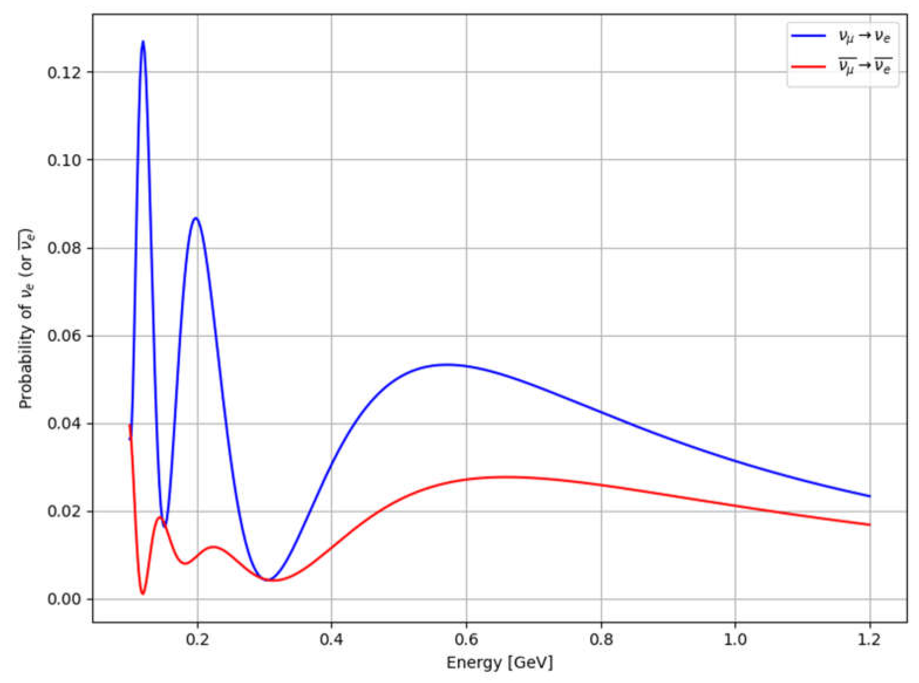
When the propagation distance is fixed at $L=295[\mathrm{k}\mathrm{m}]$, the oscillation probabilities depend on the neutrino energy (see Figure 2).

Figure 2. Relation of the neutrino energy and the neutrino oscillation probability.

Figure 2. Relation of the neutrino energy and the neutrino oscillation probability.

4.3.2. Energy Distribution of the Muon (Anti-)Neutrino Beam

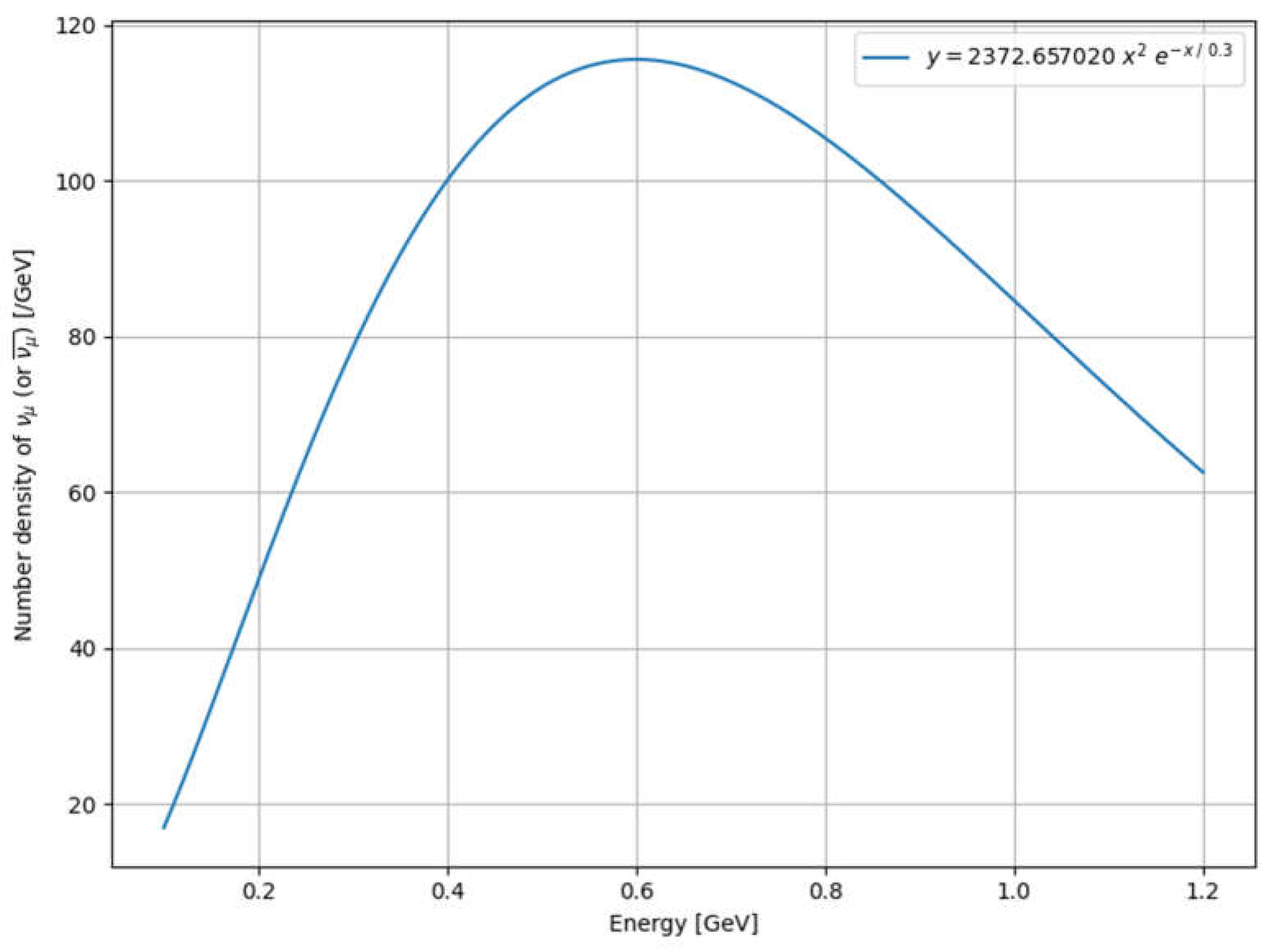
Based on the experimental setup, the energy of the emitted ${\nu }_{\mu }$ (or $\overline{{\nu }_{\mu }}$) beam is not precisely $0.6[\mathrm{G}\mathrm{e}\mathrm{V}]$ but instead exhibits a spread in its distribution. Although I do not know the exact form of the beam energy distribution, I assume, for example, that it can be represented by a function such as:

$y=2446.048140·x^2·{\mathrm{e}}^{-{\displaystyle \frac{x}{0.3}}}$,

where $x[\mathrm{G}\mathrm{e}\mathrm{V}]$ represents the beam energy and $y[/\mathrm{G}\mathrm{e}\mathrm{V}]$ denotes the number density of the emitted ${\nu }_{\mu }$ (or $\overline{{\nu }_{\mu }}$). This distribution is shown in Figure 3.

The function has its peak value at $x=0.6$.

The expected number of emitted ${\nu }_{\mu }$ (or $\overline{{\nu }_{\mu }}$) in the energy range $0.1-1.2[\mathrm{G}\mathrm{e}\mathrm{V}]$ is given by:

${\int }_{0.1}^{1.2}ydx\approx 100.000000$.

Figure 3. Relation of the neutrino beam energy and the number density of ${\nu }_e$ (or $\overline{{\nu }_e}$.)

Figure 3. Relation of the neutrino beam energy and the number density of ${\nu }_e$ (or $\overline{{\nu }_e}$.)

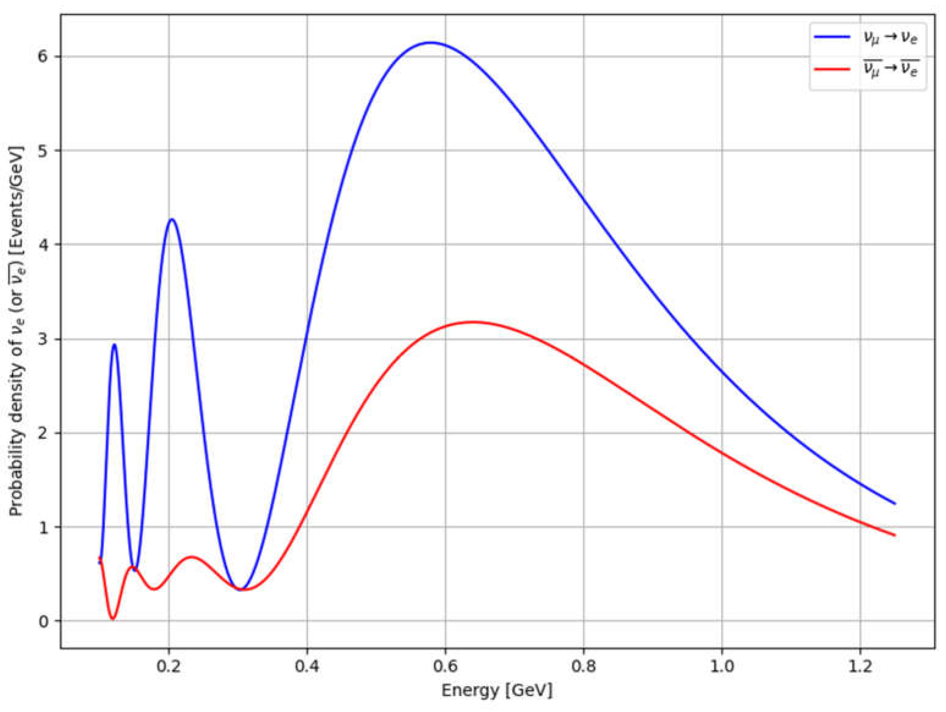
4.3.3. Probability Density and Expected Number of (Anti-)Neutrinos

By combining the two functions, the probability density for ${\nu }_e$ (or $\overline{{\nu }_e}$) is obtained, as shown in Figure 4.

The shape of the graph in Figure 4 seems similar to the graph in the paper by the T2K Collaboration [13].

By integrating over the range $0.1-1.2[\mathrm{G}\mathrm{e}\mathrm{V}]$, the expected number of events can be estimated as follows:

Out of 100 observed neutrinos, the expected number of ${\nu }_e$ is:

approximately $3.921568[\mathrm{E}\mathrm{v}\mathrm{e}\mathrm{n}\mathrm{t}\mathrm{s}]$.

Out of 100 observed antineutrinos, the expected number of $\overline{{\nu }_e}$ is:

approximately $2.023572[\mathrm{E}\mathrm{v}\mathrm{e}\mathrm{n}\mathrm{t}\mathrm{s}]$.

However, various other conditions are involved in actual observations, making it difficult for an individual to verify whether the derived values of the PMNS matrix are correct.

Future research findings in the future are awaited.

Figure 4. Relation of the neutrino energy and the probability density of ${\nu }_e$ (or $\overline{{\nu }_e}$.)

Figure 4. Relation of the neutrino energy and the probability density of ${\nu }_e$ (or $\overline{{\nu }_e}$.)

5. Conclusion

Assuming the correctness of Koide’s mass formula and Carl A. Brannen’s neutrino mass hypothesis, two three-dimensional mass models were constructed.

As a result, I discovered that the PMNS matrix can be derived by introducing an intermediate set of hypothetical states, referred to as mass negative eigenstates, which mediate the transformation between mass eigenstates and flavor eigenstates.

Based on this proposal, the PMNS matrix is derived as follows:

${\mathit{U}}_{\mathrm{P}\mathrm{M}\mathrm{N}\mathrm{S}}\approx \left[\begin{array}{ccc}0.804241& 0.577350& -0.140935\mathrm{i}\\ -0.402120-0.122054\mathrm{i}& 0.577350& 0.696493+0.070468\mathrm{i}\\ -0.402120+0.122054\mathrm{i}& 0.577350& -0.696493+0.070468\mathrm{i}\end{array}\right]$.

Whether this PMNS matrix and the neutrino oscillation expectations derived from it are correct remains to be verified by future research findings.

References

- Koide, Y. “Fermion-Boson Two Body Model of Quarks and Leptons and Cabibbo Mixing. ” Lettere al Nuovo Cimento 1982, 34, 201–206. [Google Scholar] [CrossRef]
- Koide, Y. “A Fermion-Boson Composite Model of Quarks and Leptons. ” Physics Letters B 1983, 120, 161–165. [Google Scholar] [CrossRef]
- Harari, H. , Haut, H. , & Weyers, J. “Quark Masses and Cabibbo Angles.” Physics Letters B 1978, 78, 459–461. [Google Scholar]
- Brannen, C. A. (2006). “The Lepton Masses.” Brannen Works, Retrieved from https://brannenworks.com/MASSES2.pdf.
- Amsler, C. , et al. (Particle Data Group). “Review of Particle Physics.” Physics Letters B 2008, 667, 1–1340. [Google Scholar] [CrossRef]
- Maki, Z. , Nakagawa, M. , & Sakata, S. “Remarks on the Unified Model of Elementary Particles.” Progress of Theoretical Physics 1962, 28, 870–880. [Google Scholar] [CrossRef]
- Christenson, J. H. , Cronin, J. W., Fitch, V. L., & Turlay, R. “Evidence for the 2π Decay of the Meson.” Physical Review Letters 1964, 13, 138–140. [Google Scholar] [CrossRef]
- Kobayashi, M. , & Maskawa, T. “CP-Violation in the Renormalizable Theory of Weak Interaction.” Progress of Theoretical Physics 1973, 49, 652–657. [Google Scholar] [CrossRef]
- Harrison, P. F. , Perkins, D. H., & Scott, W. G. “Tri-Bimaximal Mixing and the Neutrino Oscillation Data.” Physics Letters B 2002, 530, 167–173. [Google Scholar] [CrossRef]
- Esteban, I. , Gonzalez-Garcia, M. C., Maltoni, M., Schwetz, T., & Zhou, A. (2024). “Leptonic Mixing Matrix.” NuFIT 5.3, Retrieved from http://www.nu-fit.org/?q=node/278.
- Pontecorvo, B. (1957). “Inverse Beta Processes and Nonconservation of Lepton Charge.” Zhurnal Éksperimental’noĭ i Teoreticheskoĭ Fiziki 1957, 34, 247–250. Reproduced and translated in Soviet Physics JETP 1958, 7, 172–175. [Google Scholar]
- Abe, K. , et al. (T2K Collaboration) (2017). “Measurement of Neutrino Oscillation Parameters from the T2K Experiment.” Physical Review Letters 2017, 118, 151801. [Google Scholar] [CrossRef]
- T2K Collaboration. (2023). “Search for CP Violation in Neutrino Oscillations.” Preprint available at arXiv:2310.11942v2.
Disclaimer/Publisher’s Note: The statements, opinions and data contained in all publications are solely those of the individual author(s) and contributor(s) and not of MDPI and/or the editor(s). MDPI and/or the editor(s) disclaim responsibility for any injury to people or property resulting from any ideas, methods, instructions or products referred to in the content. |
© 2025 by the authors. Licensee MDPI, Basel, Switzerland. This article is an open access article distributed under the terms and conditions of the Creative Commons Attribution (CC BY) license (https://creativecommons.org/licenses/by/4.0/).
Copyright: This open access article is published under a Creative Commons CC BY 4.0 license, which permit the free download, distribution, and reuse, provided that the author and preprint are cited in any reuse.