1. Introduction
Autonomous Underwater Vehicles (AUVs), characterized by its exceptional mobility and advanced intelligence, represent a significant development in the field of ocean technology. The integration of a sophisticated navigation system which is capable of delivering precise, reliable navigation and positioning data, is fundamental for maximizing an AUV's operational efficiency and accuracy, especially when conducting missions in complex underwater environments [
1]. The commonly used underwater navigation methods for AUV mainly include dead reckoning based on inertial navigation, underwater acoustic navigation, and geophysical navigation [
2]. The underwater environment, fraught with various interferences, can unpredictably impact single-source navigation data, thus compromising the positioning accuracy and motion stability of the AUV. To mitigate these problems, AUVs often utilize integrated navigation systems, incorporating an array of sensors such as electronic compasses, Doppler Velocity Logs (DVLs), GPS receiver, Ultra-Short Baseline (USBL) systems, and Inertial Navigation Systems (INSs) [
3]. By applying filtering algorithms, INSs fuse and optimize navigation information from multiple sources, enhancing the overall stability and accuracy of the AUV’s positioning capability [
4].
In the latter half of the 20th century, technological limitations were a significant factor in the early stage of AUV development. At that time, the overall size of the AUV as well as the high-power consumption and cost of the navigation system made it challenging for widespread use [
5]. Therefore, the related research primarily focused on the optimization of the system hardware construction and cost reduction. In the Autonomous Minehunting and Mapping Technologies Program (AMMT) initiative directed by the United States Defense Advanced Research Projects Agency (DARPA), the developed AUV utilizes a Doppler-assisted navigation system that includes Doppler sonar, an inertial navigation unit (INU), and GPS [
6]. This system incorporates an enhanced Kalman filter algorithm to optimize the navigation data. During testing, this system achieved a positioning accuracy of nearly 0.02% of the overall travel distance. Larsen has combined sensor units including Ring Laser Gyro (RLG), DVL, INS, Short Baseline (SBL), and GPS receiver to create the MARPOS navigation system, which has been applied to the Mardian range of commercial AUVs after extensive testing to prove its reliability and accuracy [
7]. Under the impetus of the ‘863’ project, China developed the first 6000-meter-class AUV "CR-01" in 2001 [
8]. The navigation system of the AUV combined INS, DVL and Long Baseline (LBL), which was able to control the positioning error in 10 meters within the coverage area of the LB positioning system. The AUV successfully completed two research missions on the investigation of manganese nodules at the bottom of the Pacific Ocean.
With advances in technology and further improvements in the hardware of navigation system, significant advances in battery technology have enabled AUVs to perform underwater tasks for extended periods of time, far beyond the capabilities of traditional manned submersibles or Remotely Operated Vehicle (ROV). However, the increased duration and scope of these missions has necessitated greater precision in navigation system [
9]. Zhang et al. have provided a comprehensive review and summary of the composition and development history of AUV navigation systems since the 1980s [
10]. The technologies employed in AUV navigation are currently transitioning from traditional methods requiring the preliminary deployment of positioning devices like LBL and USBL to approaches that utilize dynamic multi-agent systems. Emerging navigation techniques such as Simultaneous Localization and Mapping (SLAM) are enabling significant enhancements in both the cost-effectiveness and accuracy of AUV navigation [
11].
The central issue in the field of AUV navigation is the state estimation [
12]. In order to achieve improved and more consistent positioning performance, study on integrated navigation systems is increasingly focusing on enhancing nonlinear filtering algorithms within the software framework. The Kalman filter (KF) is the most commonly used filtering algorithm for processing problems related to multi-sensor data fusion in the navigation field [
13]. The KF algorithm was often used in early AUV navigation systems to achieve the data fusion between different hardware components [
14]. In order to better dealing with the nonlinear system filtering problem, various different nonlinear filtering algorithms have been further developed on the basis of the KF algorithm. The Extended Kalman filter (EKF) algorithm is a common algorithm derived from the Kalman filter, which is widely used in AUV navigation systems by linearizing and approximating the nonlinear term with a Taylor's first-order expansion. It’s particularly effective for systems that exhibit mild nonlinearity and non-Gaussian characteristics, hence its widespread use in the integrated navigation system of AUV [
15]. Fulton et al. used the REMUS AUV to test the EKF algorithm by post-processing the data collected by acoustic navigation system, Doppler sonar and compass mounted on the AUV [
16]. Their algorithm extends the EKF by integrating a feature that autonomously detects and removes outliers. The test results demonstrated that the proposed algorithm had consistently maintained stable performance, achieving positioning accuracy with an error margin within a few meters.
The EKF algorithm has the advantages of easy implementation and faster operation speed. However, the method of linearizing the nonlinear terms through the first-order Taylor expansion has a certain error, which may lead to further increasing or even dispersion of the filtering error when dealing with strongly nonlinear systems. To enhance the navigation accuracy, several studies have attempted to combine KF with other nonlinear methods. To address these limitations and enhance the performance of EKF in AUV navigation, Crassidis introduced an advanced Kalman filtering approach named the Sigma Point Kalman filter (SPKF), which specifically aims to optimize the fusion of GPS and INS data [
17]. Similar to the SPKF, the Unscented Kalman filter (UKF) is a nonlinear filtering algorithm that applies the unscented transform to the KF, which has been proven to be more accurate and easier to implement than EKF in nonlinear estimation [
18,
19]. On this basis, Krauss et al. proposed an unscented Kalman filter algorithm on manifolds (UKF-M), which added an additional step of identifying and eliminating the outliers of the sensor measurements in the process of state updating [
20]. Experiments demonstrated that the method can not only effectively attenuate the influence of outliers on AUV speed estimation but also improving the convergence ability of heading estimation. In addition, the Particle Filter (PF) serves as another prevalent nonlinear filtering technique [
21]. It employs the principles of the Monte Carlo method, utilizing a collection of particles to perform stochastic sampling and weight allocation, thereby representing the system's probability density distribution [
22]. This method facilitates the estimation of the system state without the need for deriving analytical solutions [
23].
Similar to PF, the Ensemble Kalman filter (EnKF) is a nonlinear filtering algorithm that combines KF with Monte Carlo method. EnKF constructs a sample ensemble to take the place of the covariance matrix operation in KF, which enhances the filter's effectiveness in dealing with nonlinear systems, offering significant improvements in handling the inherent complexity of such models. It uses a finite set of states to approximate the statistical properties of the system states, implicitly estimating the error covariance matrix through the variance between the sample ensembles. This approach avoids the direct manipulation of large error covariance matrices encountered in the conventional KF algorithm on large systems, and significantly reduces the computational resource consumption when dealing with high-dimensional systems [
24]. Due to its great ability to handle high-dimensional nonlinear systems, EnKF is now widely used in the field of meteorological model prediction [
25].
Cui and Zhang attempted to apply the EnKF algorithm to address the issue of multi-sensor target tracking [
26]. Through empirical testing, it was demonstrated that the EnKF method outperforms the conventional Extended Kalman filter (EKF) method in dealing with issues of multi-sensor target tracking, confirming its effectiveness for use in AUV navigation systems. Pornsarayouth et al. integrated the one-step smoothing method with the EnKF method to address the issue of multi-sensor target positioning [
27]. Simulation results demonstrated that the EnKF method outperforms traditional methods such as EKF and PF, in handling issues associated with ‘out-of-sequence’ (OOSE) measurements in integrated navigation systems. Tin et al. have conducted extensive research on the application of EnKF in AUV underwater navigation [
28]. They independently applied KF, EnKF and the Fuzzy Kalman filter (FKF) to AUV navigation data, evaluated the performance based on computation time and the root mean square error (RMSE) of positioning. The results demonstrated that EnKF outperforms FKF in both computational efficiency and three-dimensional positioning accuracy [
29]. They conducted simulations of AUV motion in three-dimensional space to evaluate the positioning performance of EnKF over different ensemble member sizes. Experimental results showed that EnKF maintained consistently low average positioning errors. Furthermore, as the number of ensemble members increases, the positioning accuracy of the algorithm improves, albeit at the cost of reduced computational speed [
30].
EnKF has been demonstrated to be effective in AUV integrated navigation system, but it still has notable limitations. First, the EnKF algorithm replaces traditional covariance matrix operations with statistical analyses of randomly generated sample ensembles. The outcomes of this method are significantly influenced by the number and mathematical properties of these samples, resulting in a filter output that exhibits instable variability. In comparison to conventional KF or EKF approaches, EnKF exhibits less smoothness and stability in its filtering trajectory. Secondly, although EnKF can effectively handle the nonlinear systems, its stability may degrade under common non-Gaussian noise disturbances in marine environments. To address these issues, improvements to the EnKF algorithm should start from the sample ensemble generation. This involves enhancing the algorithm's stability by modifying the sample generation process and dynamically adjusting the number of samples in the ensemble. By balancing precision and efficiency, these modifications aim to optimize overall filtering performance.
This paper proposes an enhanced adaptive EnKF algorithm for AUV integrated navigation. The highlights of the enhanced algorithm include:
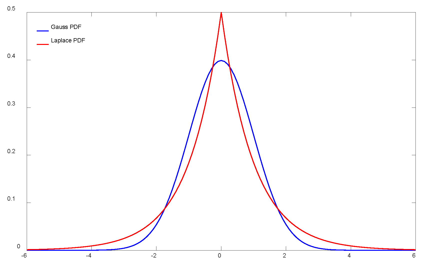
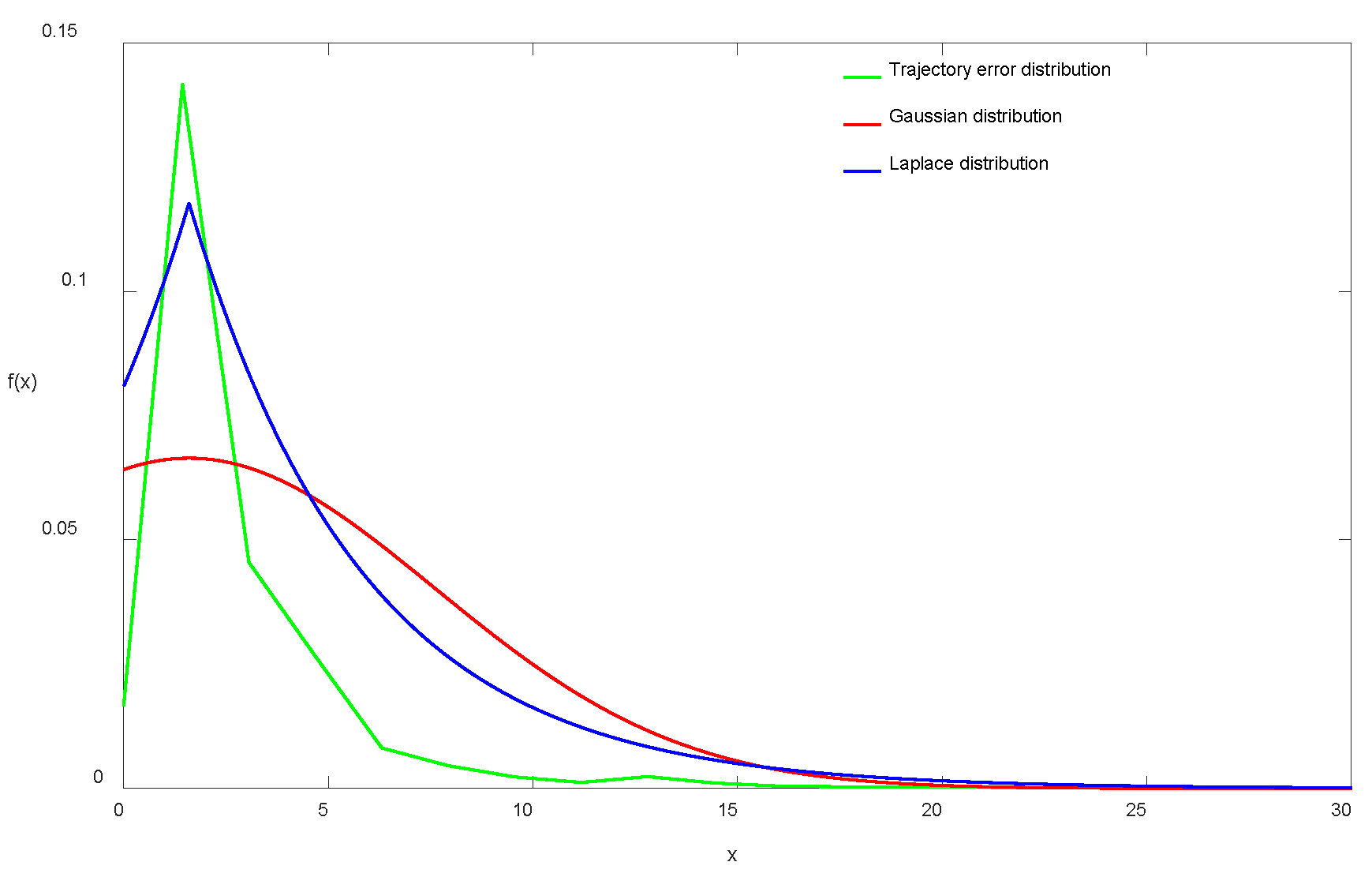
(1) The algorithm employs the Laplace distribution instead of the conventional Gaussian distribution to generate members of state vector ensembles. The general behavior of the Laplace distribution resembles the Gaussian distribution but includes a higher incidence of outliers. This feature allows the algorithm to more closely mimic the real system state in natural environments, thereby improving the algorithm's robustness to non-Gaussian noise.
(2) The adaptive mechanism allows the algorithm to dynamically adjust the number of members in the state vector ensemble based on an evaluation of the smoothness of the filtered trajectory and the credibility of filtering outputs. This enables the algorithm to adaptively modify its performance according to the actual demand on smoothness and accuracy, thus enhancing the efficiency for real-time navigation.
(3) AUV navigation data obtained from field tests were used for the parameter optimization and performance validation of our proposed filtering algorithm. The advantages of the enhanced adaptive EnKF algorithm were demonstrated through comparisons with other filtering algorithms.
The rest of this paper is organized as follows.
Section 2 introduces the AUV platform and the hardware configuration of its integrated navigation system in this study.
Section 3 presents the model and the parameters involved in our proposed EnKF algorithm, and also describe our sample generation method derived from the Laplace distribution. In section 4, the key parameters of the algorithm are tuned based on AUV field data to optimize algorithmic performance.
Section 5 introduces our adaptive mechanism into the algorithm, enabling it to adjust the number of generated sample ensembles based on the smoothness of the filtered trajectory curves and the credibility of filtering outputs. We detail of the comparison between our enhanced EnKF algorithm with standard algorithms such as the conventional EnKF and EKF in
Section 6. The last section summarizes the findings in the research and the future directions.
5. Adaptive Mechanism in EnKF
The previous section investigated the impacts of various algorithm parameters on its filtering performance and achieved parameter optimization by selecting the optimal configurations. In addition to the parameters discussed in
Section 4, the number of random samples included in the state vector ensemble generated by the algorithm also influences filtering stability and operational efficacy. The size of this ensemble dictates the sampling density within the system’s state space. Increasing the number of vector samples with random perturbations enhances the model's ability to approximate the system’s uncertainties and nonlinear features. However, this also increases computational and storage demands, thereby increasing the runtime. Conversely, a smaller ensemble of state vector samples may not adequately represent the system's complexity and uncertainty, potentially compromising the algorithm's filtering stability. Building on the preceding discussion, this subsection introduces an adaptive mechanism to the EnKF algorithm.
5.1. Key Criteria of Adaptive Mechanism
Our proposed mechanism enables the algorithm to assess the smoothness of the filtered results and the credibility of filtering outputs based on defined criteria, then autonomously adjust the number of ensemble members in the filtering process. This allows for a dynamic equilibrium between filtering stability and real-time performance, tailored to the needs of the navigation system.
5.1.1. Smoothness of Filtering Results
The smoothness of the filtering results reflects the extent of noise reduction and the accuracy of trajectory estimation. Smoother filtering outcomes indicate that the algorithm effectively mitigates noise and accurately captures the true motion pattern of the AUV, resulting in more reliable and stable trajectory predictions.
To evaluate the smoothness of the filtering results, we define a smoothness angle, which is the angle between two lines connecting adjacent trajectory points of the AUV after the filtering process. By computing the average angle of all trajectory points within a specified time interval, we can assess the smoothness of the filtered trajectory. The angle between every three consecutive trajectory points can be determined using the dot product of the corresponding vectors:
where
represent three consecutive trajectory points,
and
are the vectors defined by these points, and
is the angle between the two vectors. Assume that AUV trajectory point estimated by the EnKF algorithm at time
are
, and the trajectory points at times
and
are
and
, respectively. Consequently, the following expression can be derived from Equation (26):
where
denotes the angle with respect to the trajectory point at time step
after filtering.
With Equation (27), we can record the smoothness angle at each trajectory point prior to time . This angle serves as an indicator of the local smoothness of the filtering trajectory at that point. The angle ranges from 0° to 180°, with values closer to 180° indicating better smoothness of the trajectory. By calculating the average smoothness angle of all trajectory points within a specified time interval, we can evaluate the smoothness of the filtering results.
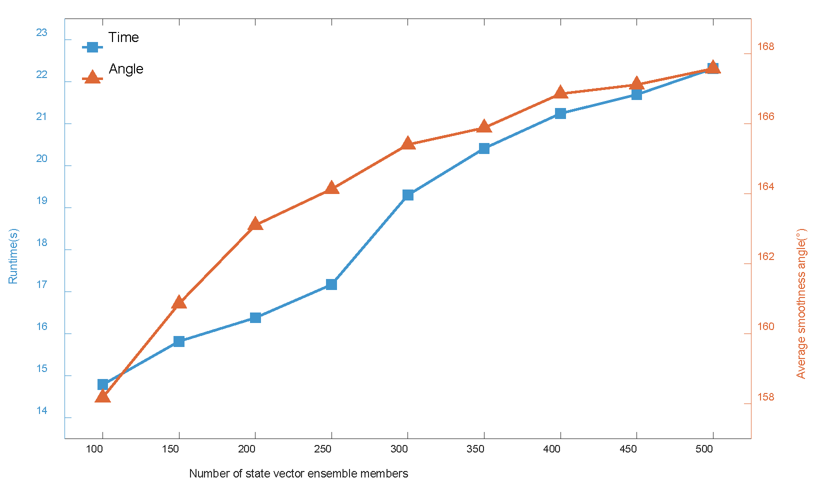
In our study, we find that the number of state vector ensemble members significantly impacts the smoothness of the filtering results. Generally, a larger number of ensemble members leads to a smoother filtered trajectory, but this also increases the filtering runtime, potentially compromising the real-time performance of the filter for online operation. With the given dataset, the variation in runtime and the average smoothness angle of the filter over a specified time period with the number of state vector ensemble members is depicted in
Figure 12. The dataset comprises 30,000 sampling points, each separated by approximately 0.2 s, resulting in a total duration of approximately 600 s. As illustrated in
Figure 12, an increase in the number of state vector ensemble members results in a smoother filtered trajectory. However, this also leads to a significant increase in the runtime of the filtering algorithm.
Based on the method for assessing the smoothness of filtering results mentioned above, an adaptive adjustment approach is integrated into the algorithm to dynamically alter the number of state vector members in the ensemble based on predefined thresholds. During the filtering process, a sliding window is used to average a specified number of smoothness angles along the filtered trajectory. This average serves as the quantitative measure of the trajectory’s smoothness. If it exceeds an upper threshold, indicating a sufficiently smooth trajectory, the algorithm will decrease the size of the generated state vector ensemble, thereby expediting the processing speed. Conversely, if the average smoothness angle falls below a lower threshold, suggesting substantial fluctuations in the trajectory, the number of ensemble members will be increased to enhance filtering accuracy.
5.1.2. Credibility of Filtering Outputs
When the AUV persists in moving along relatively straight paths, the algorithm, influenced by the smoother trajectory points, may consistently generates fewer ensemble members. This could impede the algorithm's capacity to implement prompt and effective corrections to minor deviations that occur during movement, thereby gradually leading to the accumulation of filtering errors.
To address this issue, we further introduce a refined approach for adjusting the number of ensemble members based on the credibility of the filtering outputs. This approach establishes a threshold and calculates the Euclidean distance between the dead reckoning positioning data and GPS data, as specified in Equation (28):
where
and
denote the positional coordinates derived from dead reckoning and GPS measurements, respectively;
represents the Euclidean distance deviation between them. If
is found to be significantly large and persists above the threshold
for a specified duration, it indicates a substantial deviation between the dead reckoning positioning data and the GPS data. In such cases, it is necessary to increase the number of ensemble members in order to maintain algorithmic precision. Conversely, if
decrease and remain below the threshold for a certain period, the method reduces the number of ensemble members. The determination of the threshold
, the increment in member numbers once this threshold is surpassed, as well as the upper limit of the increase, should be tailored to the specific requirements of the navigation task and the scale of the mission area.
5.2. Validation of Adaptive Mechanism
To validate the filtering performance of the EnKF algorithm enhanced with the adaptive mechanism described above, a comparative analysis is conducted between the EnKF algorithm before and after implementing this adaptive mechanism. The comparative analysis involved the following four scenarios of the EnKF algorithm, each applied to filter and assess navigation data:
A. EnKF with a constant ensemble size of 250;
B. EnKF adaptively adjusting the ensemble size based on both the smoothness of the filtered trajectory and the credibility of the filtering outputs;
C. EnKF adaptively adjusting the ensemble size solely based on the smoothness of the filtered trajectory;
D. EnKF adaptively adjusting the ensemble size solely based on the credibility of the filtering results.
In all four scenarios, the initial ensemble size is 250, which means there are 250 state vectors in the ensemble. The ensemble size adjustment based on the smoothness of the filtered trajectory has a range of ±150, with increments of 30, while the ensemble size adjustment based on the credibility of the filtering results ranges from 0 to 100, with increments of 10. Aside from the variable ensemble size, the other parameters within the algorithm remain unchanged across the scenarios.
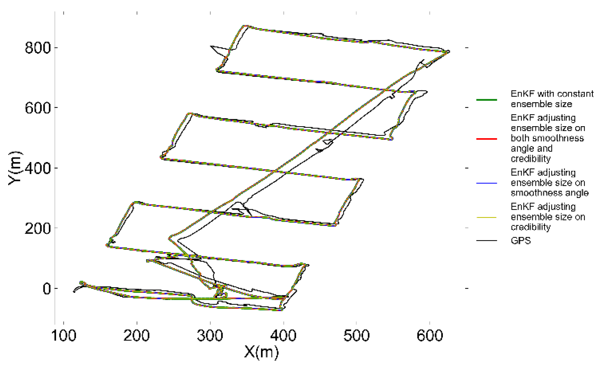
To compare the filtering performance of the four scenarios mentioned above, a series of repeated trials utilizing AUV measurements, which encompass complex motion states, are conducted. For each filtering scenario, the AUV trajectories after filtering are presented in
Figure 13. The filtering trajectories generated by the algorithm under the four scenarios demonstrate a considerable degree of overlap, making it difficult to accurately assess the precision and smoothness of the algorithm across these scenarios based solely on the curves presented in
Figure 13. This consistency is attributed to the parameter optimization described in
Section 4, which has rendered the algorithm's filtering effect on the navigation data both stable and reliable, leads to only minor differences in the positioning results across the scenarios.
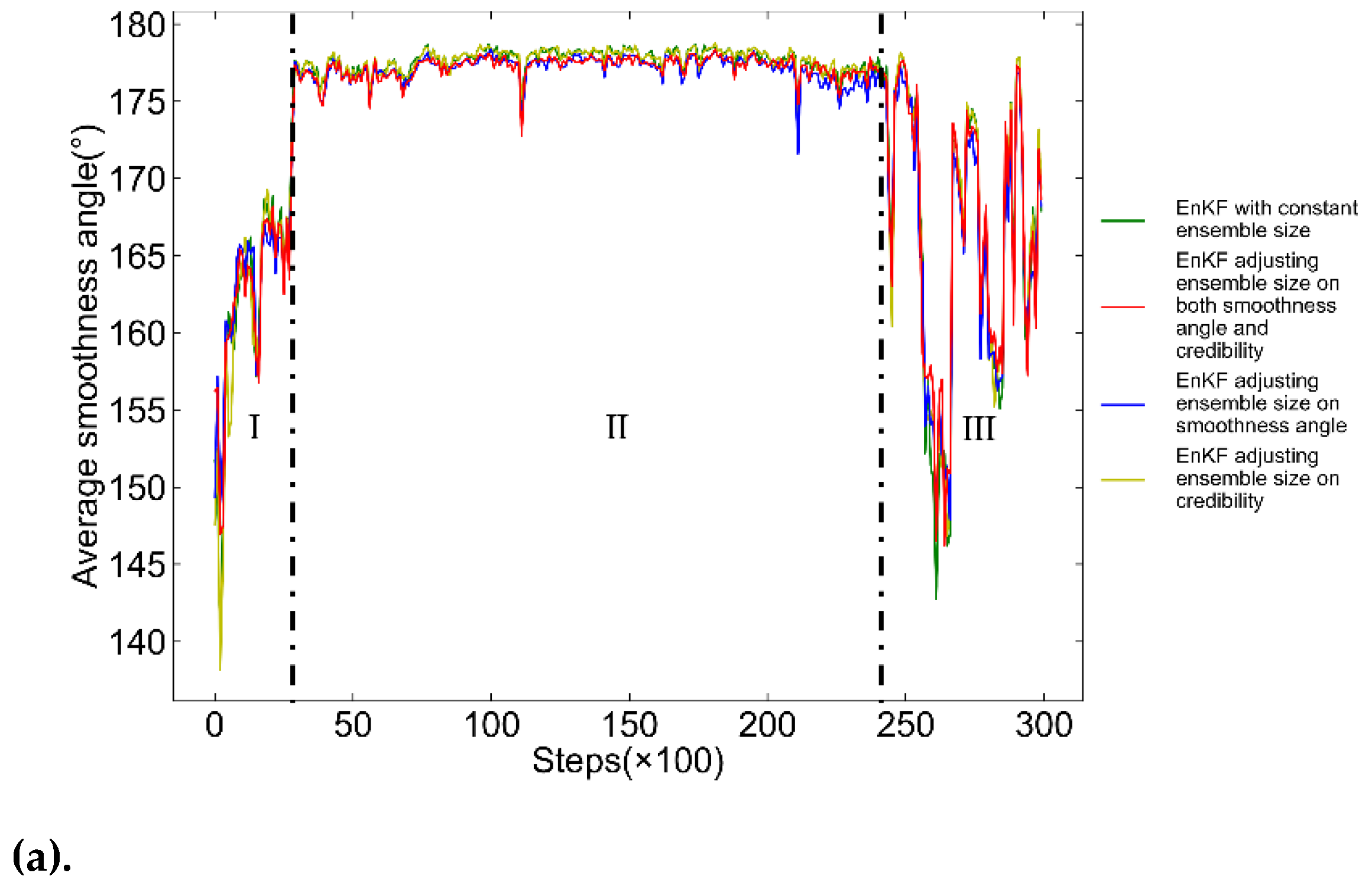
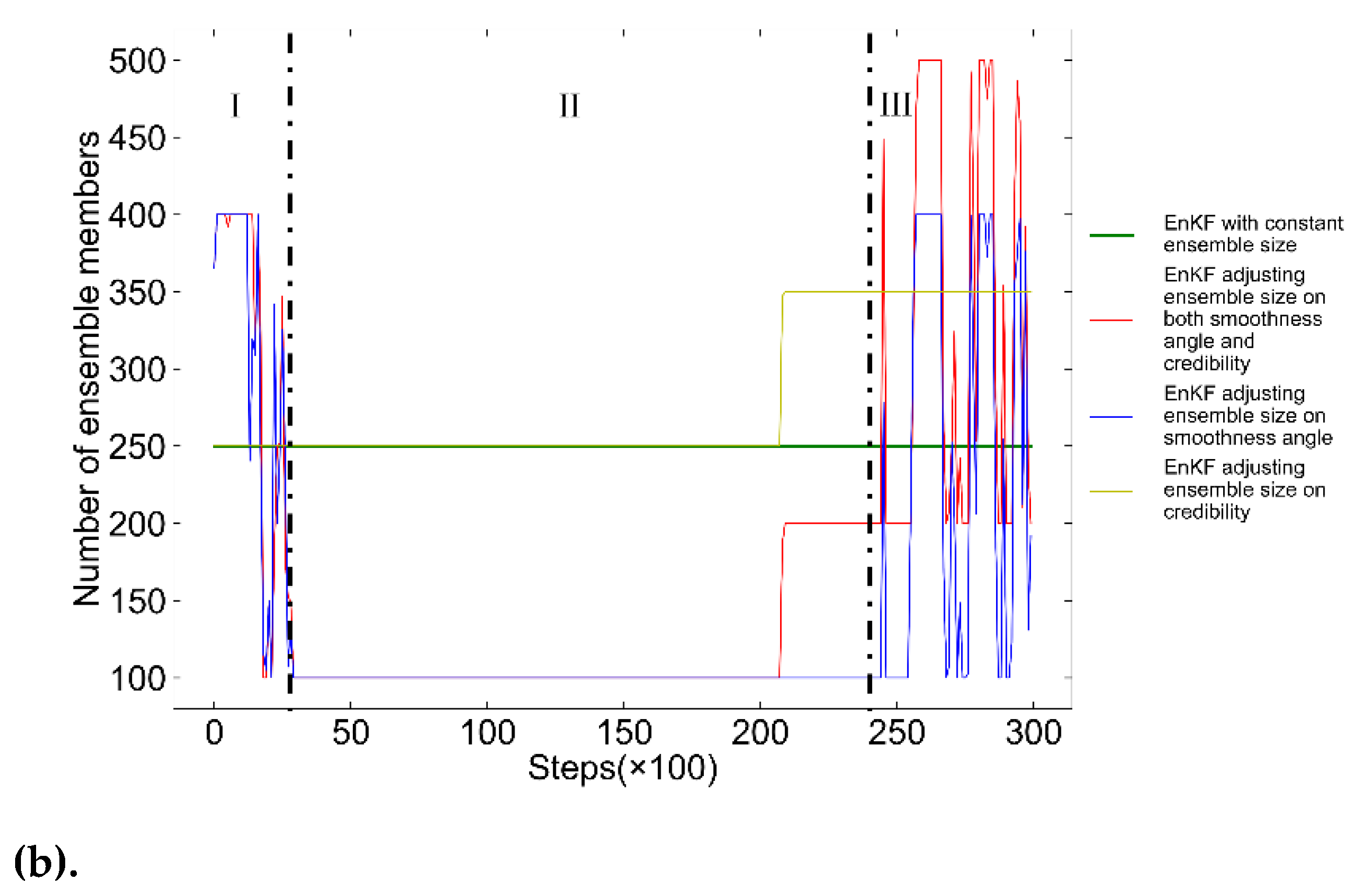
To compare the algorithm's smoothing performance under different scenarios,
Figure 14 depicts the average smoothness angle of filtered trajectories and changes in ensemble member numbers in four scenarios. The AUV trajectory is divided into three segments I, II and III based on its motion state. Segment I features complex movement with frequent attitude changes and trajectory fluctuations, leading to varying filtering smoothness, as shown in
Figure 14(a). The red and blue curves in
Figure 14(b), representing EnKF algorithm scenarios that take the smoothness of the trajectory into consideration, resulting in smoother, more stable smoothness distributions. Unlike the green and yellow curves, which drop to a local minimum smoothness angle of about 138°, the red and blue curves increase by 10°, mitigating smoothness reduction.
In Segment II, AUV demonstrates a relatively steady movement, exhibiting minimal fluctuations in trajectory smoothness. Consequently, the red and blue curves in
Figure 14(b) show a decrease in ensemble sizes, staying below the initial 250. This reduction slightly lowers the smoothness, with the red and blue curves in
Figure 14(a) showing an average smoothness angle smaller within 3° than the green and yellow curves. This indicates that moderate reducing ensemble members during stable AUV motion has little impact on filtering smoothness.
The AUV's movement in Segment III becomes complex again, causing frequent fluctuations in filtering smoothness, as shown in
Figure 14(a). The red and blue curves in
Figure 14(b) respond by frequently adjusting the ensemble sizes. The red and yellow curves, employing an adaptive mechanism based on the filtering output credibility, increase ensemble members due to growing discrepancies between dead reckoning and GPS positioning. The red curve, employing both adaptive mechanisms, effectively limits low smoothness levels, showing relatively optimal performance in
Figure 14(a) with a local minimum smoothness improvement of up to 5° compared to the other scenarios.
Furthermore, the algorithm's operational efficiency in the four scenarios was analyzed, with average runtime data presented in
Table 1. The scenario that adjusts ensemble size based on filtering smoothness, particularly during smooth AUV movement, operates significantly more efficiently than those without this adaptive mechanism. In contrast, the scenario that adapts based on the credibility of filtering outputs, increasing ensemble sizes to counter navigation errors, shows a slight increase in runtime. The red curve scenario, which adapts based on both smoothness and credibility, accelerates the filtering process, reducing iteration time by about 10% compared to the conventional EnKF algorithm. Despite this efficiency boost as well as the improvement of filtering smoothness shown in
Figure 14, there is no noticeable increase in positioning error. In practical underwater operations, as the duration of the task increases, the improvements in filtering accuracy, smoothness, and speed are expected to have an even greater impact on enhancing the AUV's positioning performance.
In conclusion, the EnKF with an adaptive mechanism for adjusting ensemble sizes based on filtering smoothness and output credibility demonstrates superior efficiency and smoothness, confirming that the proposed adaptive EnKF is better suited for real-world observational requirements and outperforms the conventional EnKF in real-time navigation.
Figure 1.
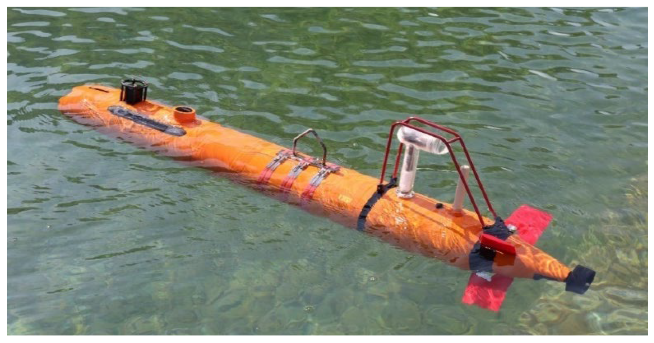
Our AUV platform.
Figure 1.
Our AUV platform.
Figure 2.
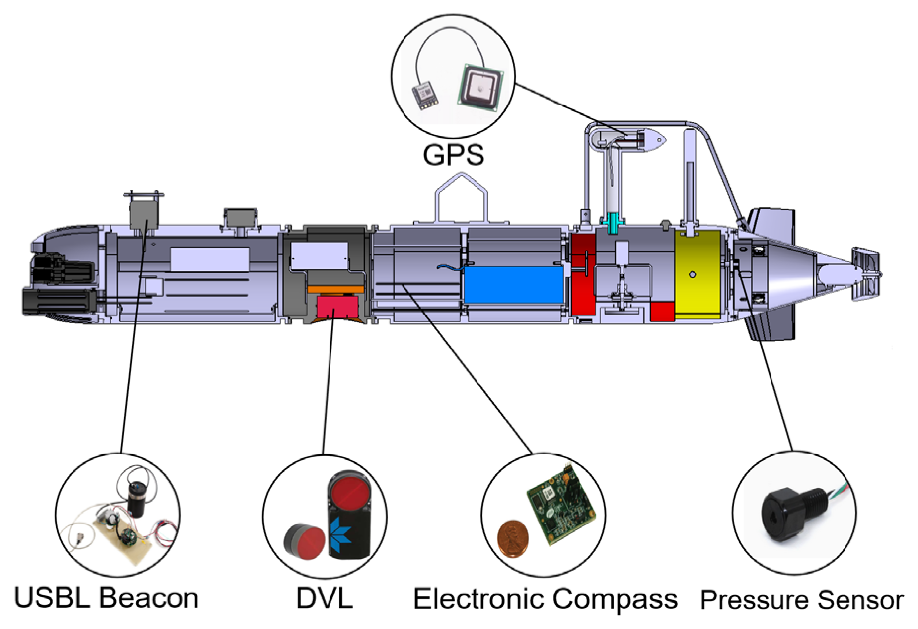
Longitudinal Sectional View of the AUV Platform Structure.
Figure 2.
Longitudinal Sectional View of the AUV Platform Structure.
Figure 3.
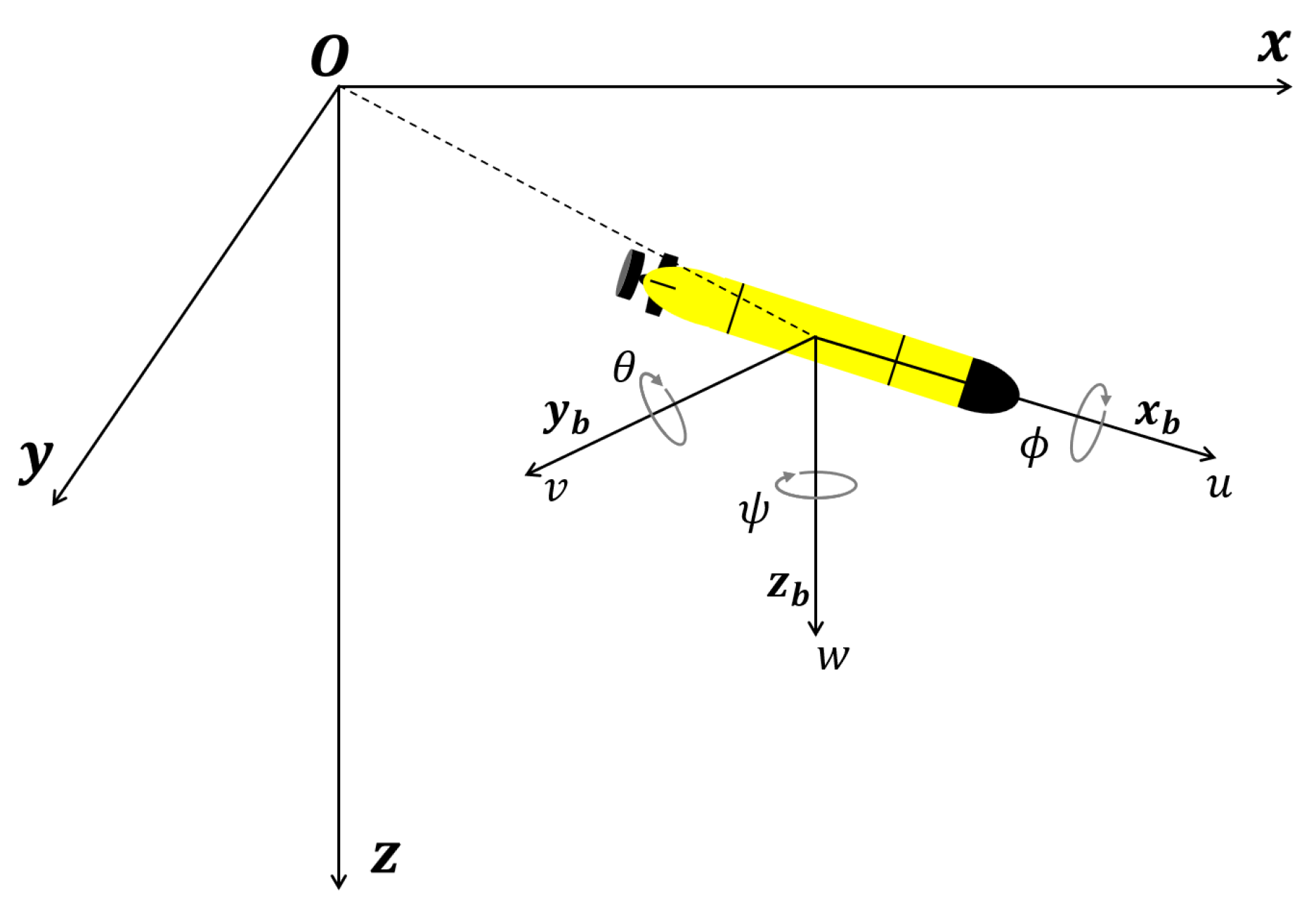
Inertial and body-fixed coordinate frames to describe AUV motion.
Figure 3.
Inertial and body-fixed coordinate frames to describe AUV motion.
Figure 4.
Comparation of the function curves for the standard Gaussian distribution () and the standard Laplace distribution ().
Figure 4.
Comparation of the function curves for the standard Gaussian distribution () and the standard Laplace distribution ().
Figure 5.
Comparison of the probability distribution of AUV positioning trajectory deviation with two theoretical probability distribution curves, the three distributions have the same mean and standard deviation.
Figure 5.
Comparison of the probability distribution of AUV positioning trajectory deviation with two theoretical probability distribution curves, the three distributions have the same mean and standard deviation.
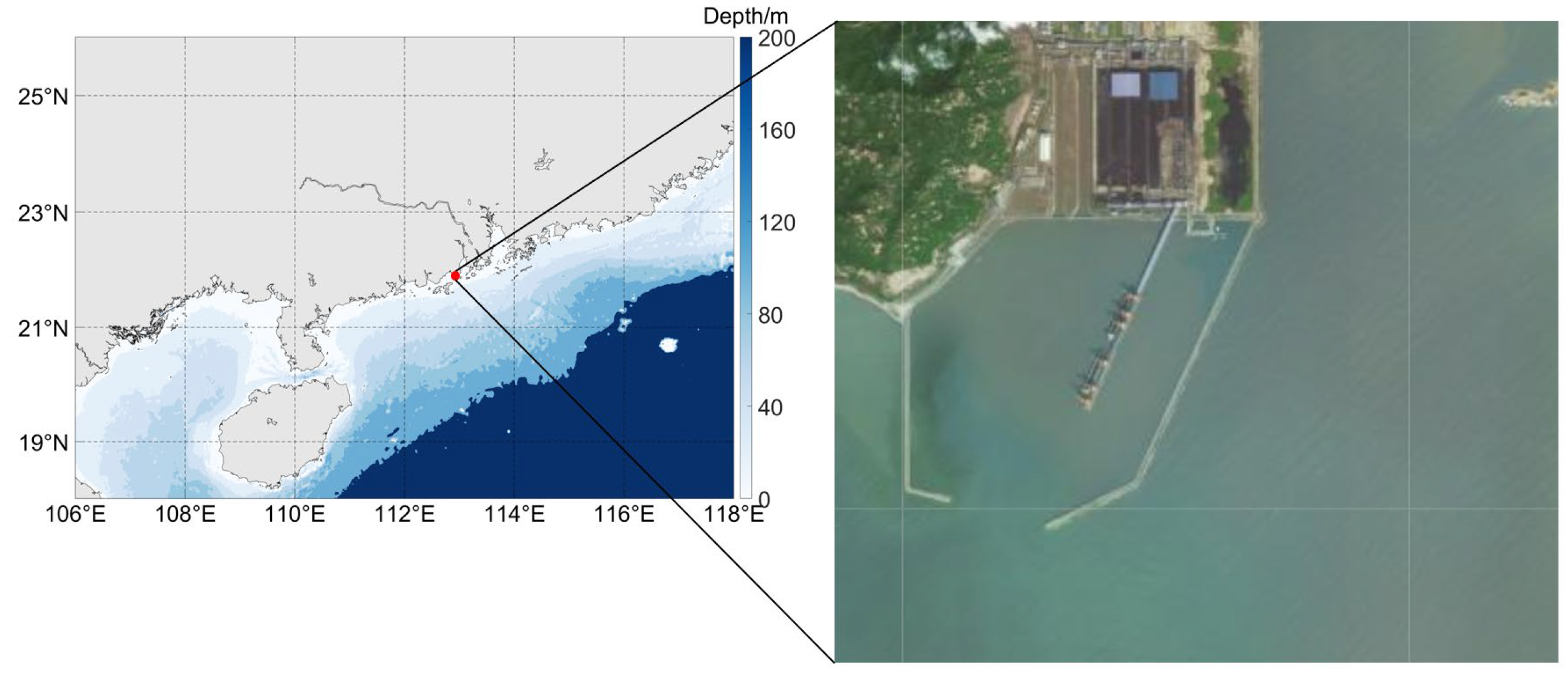
Figure 6.
Location of test area.
Figure 6.
Location of test area.
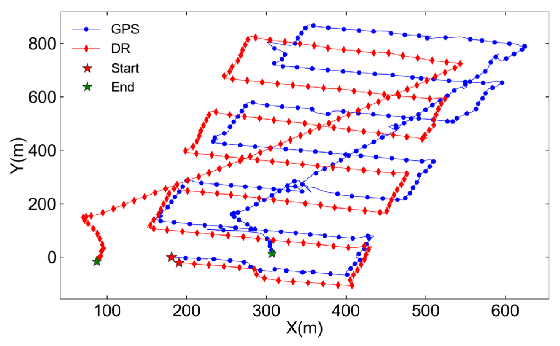
Figure 7.
Dead reckoning and GPS positioning trajectories during AUV field trial.
Figure 7.
Dead reckoning and GPS positioning trajectories during AUV field trial.
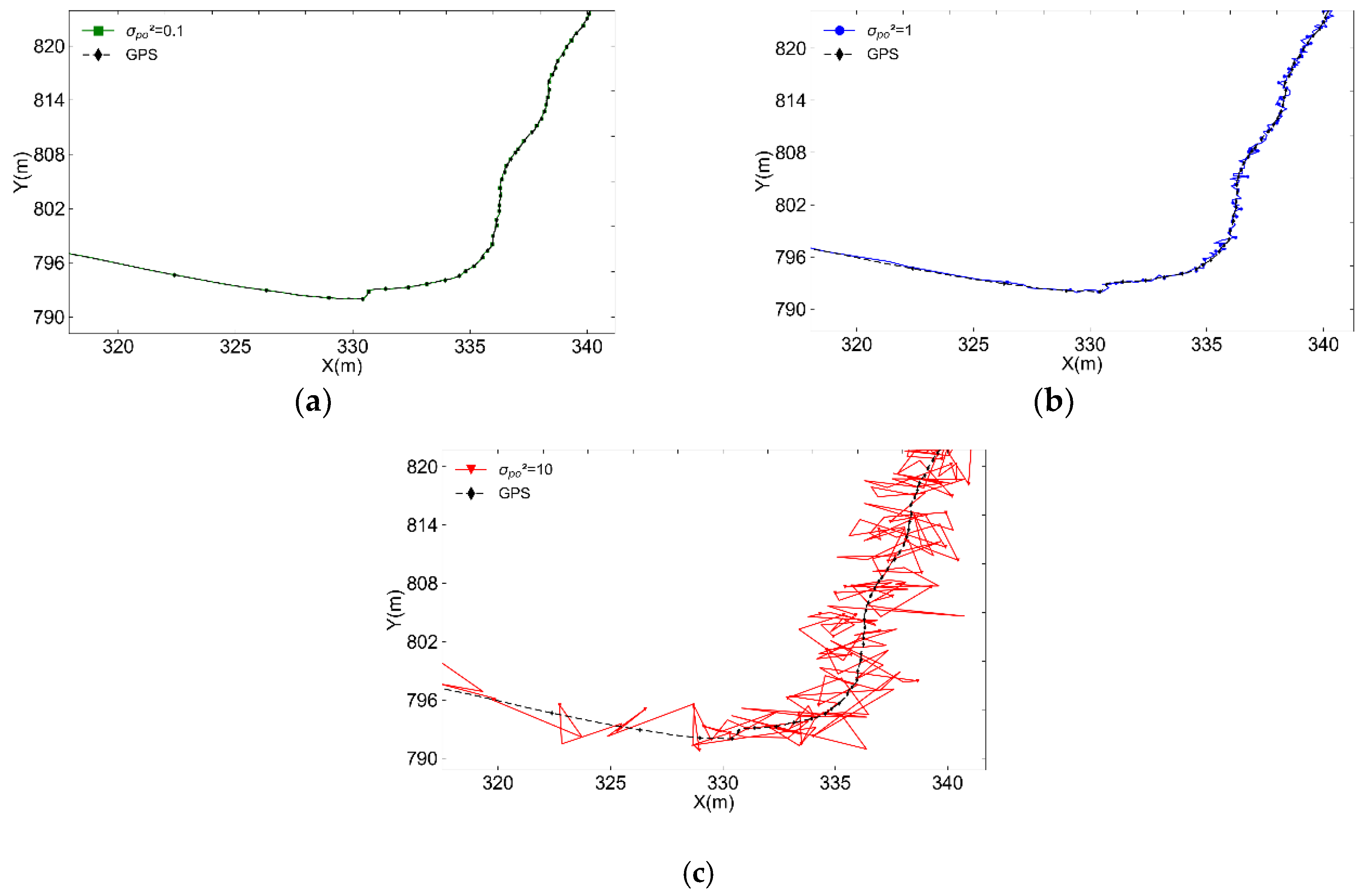
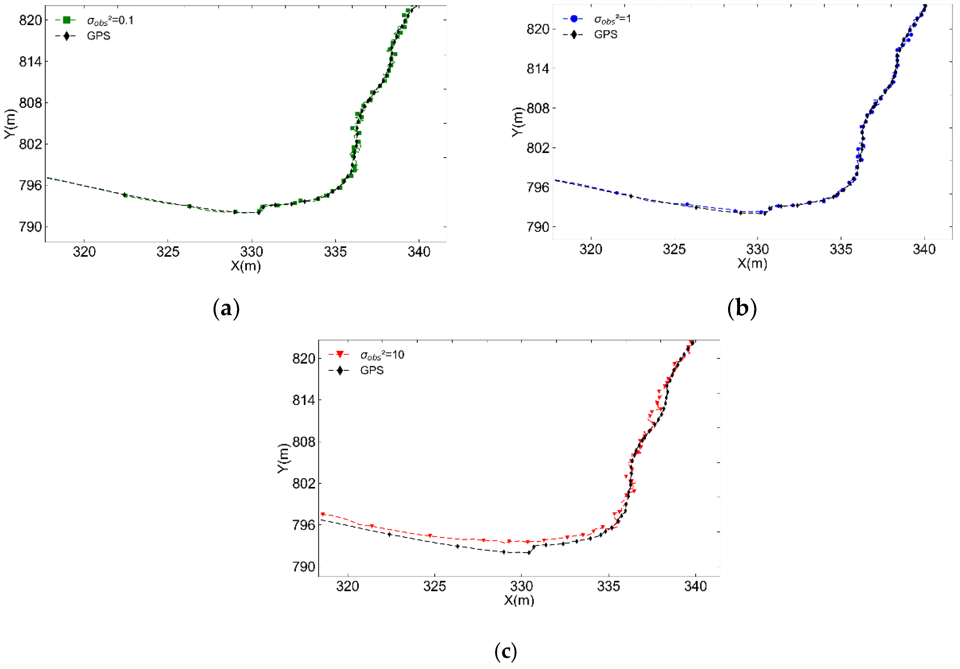
Figure 8.
Partial enlarged view of AUV trajectory during turning motion with different variance values of observation vector ensemble . (a) ; (b) ; (c) .
Figure 8.
Partial enlarged view of AUV trajectory during turning motion with different variance values of observation vector ensemble . (a) ; (b) ; (c) .
Figure 9.
Partial enlarged view of AUV trajectory during turning motion with different values of . (a) ; (b) ; (c) .
Figure 9.
Partial enlarged view of AUV trajectory during turning motion with different values of . (a) ; (b) ; (c) .
Figure 10.
AUV trajectory filtered by EnKF under different measurement noise matrix perturbation variances .
Figure 10.
AUV trajectory filtered by EnKF under different measurement noise matrix perturbation variances .
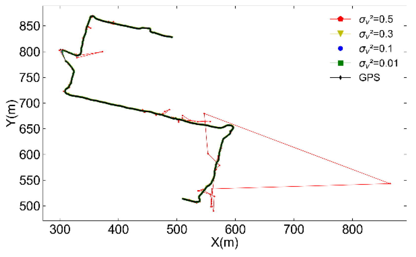
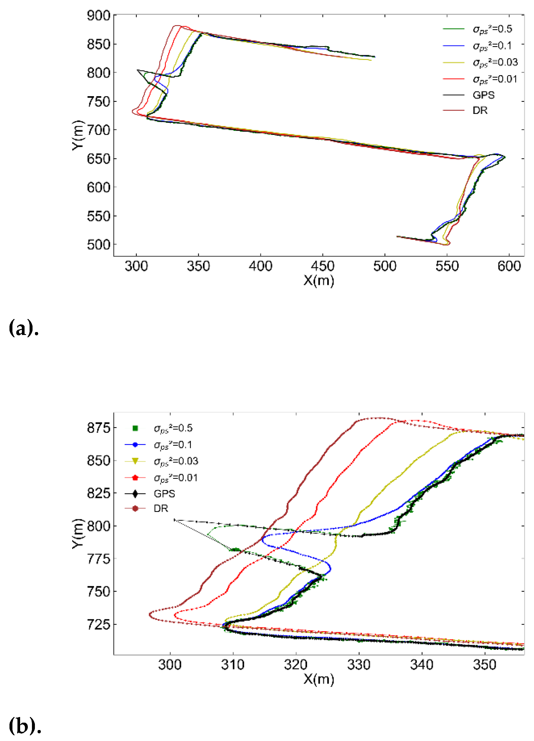
Figure 11.
Comparison of EnKF filtering trajectories with GPS and dead reckoning trajectories under different state vector ensemble. (a) Comparison of EnKF in different state vector ensemble variance values; (b) Partial enlarged view by the black box mark in
Figure 11(a).
Figure 11.
Comparison of EnKF filtering trajectories with GPS and dead reckoning trajectories under different state vector ensemble. (a) Comparison of EnKF in different state vector ensemble variance values; (b) Partial enlarged view by the black box mark in
Figure 11(a).
Figure 12.
Variation of runtime and average smoothness angle with the number of state vector ensemble members.
Figure 12.
Variation of runtime and average smoothness angle with the number of state vector ensemble members.
Figure 13.
AUV filtered trajectories in four filtering scenarios.
Figure 13.
AUV filtered trajectories in four filtering scenarios.
Figure 14.
Comparison of the number of ensemble members and average filtered smoothness angle of the algorithm in four scenarios. (a) Average smoothness angles of the filtered trajectories; (b) Alterations in the number of ensemble members of EnKF.
Figure 14.
Comparison of the number of ensemble members and average filtered smoothness angle of the algorithm in four scenarios. (a) Average smoothness angles of the filtered trajectories; (b) Alterations in the number of ensemble members of EnKF.
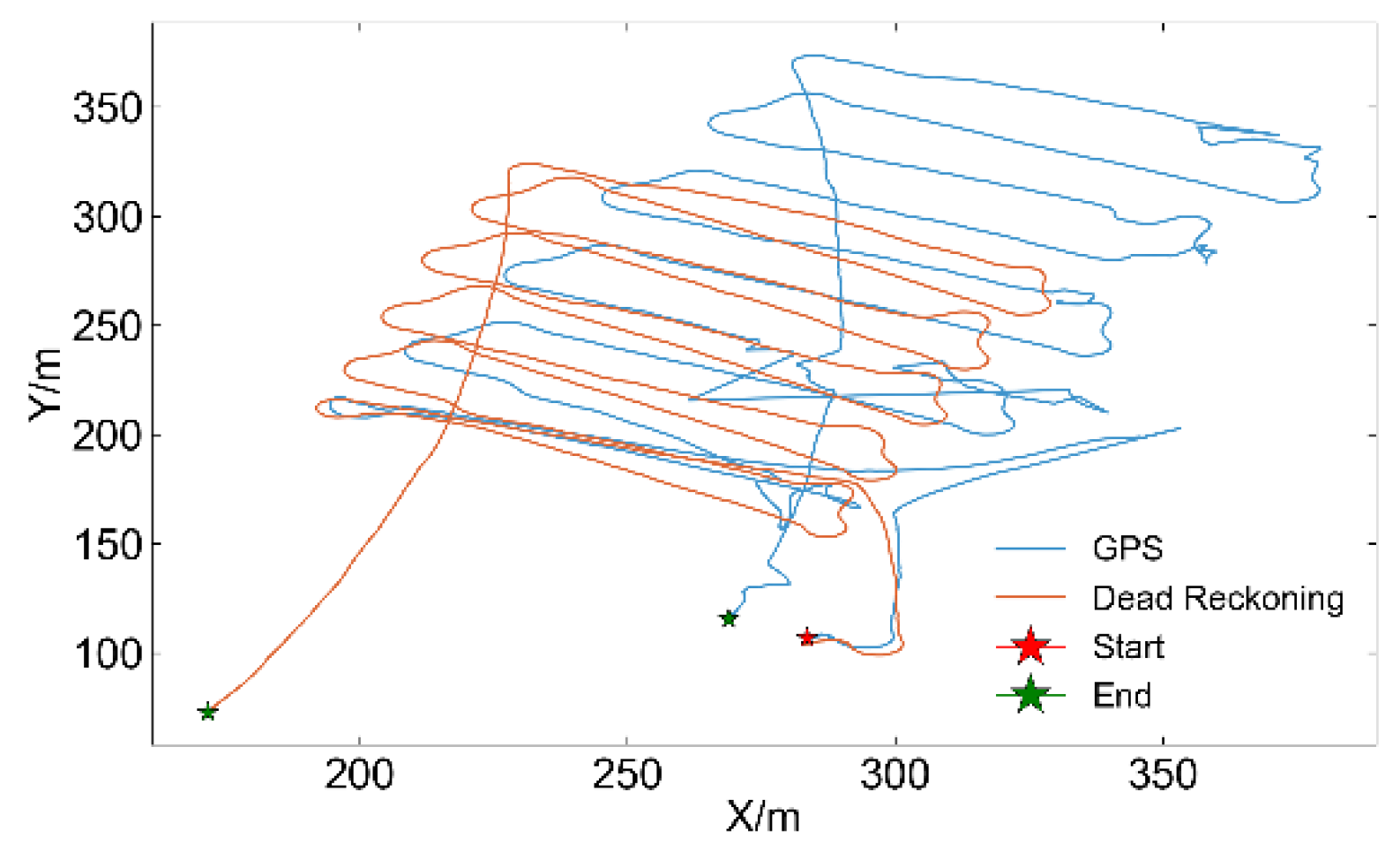
Figure 15.
Navigation data used in this section. The red asterisk indicates the starting point, and the green asterisks indicate the ending points for both GPS positioning and dead reckoning.
Figure 15.
Navigation data used in this section. The red asterisk indicates the starting point, and the green asterisks indicate the ending points for both GPS positioning and dead reckoning.
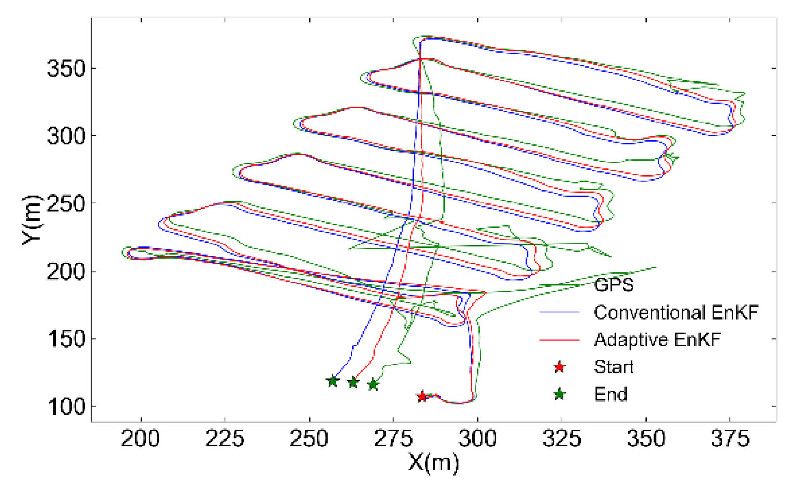
Figure 16.
Filtered trajectories by conventional EnKF and adaptive EnKF compared with GPS data.
Figure 16.
Filtered trajectories by conventional EnKF and adaptive EnKF compared with GPS data.
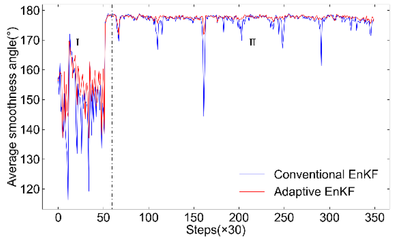
Figure 17.
Average smoothness angle distributions of conventional EnKF and adaptive EnKF.
Figure 17.
Average smoothness angle distributions of conventional EnKF and adaptive EnKF.
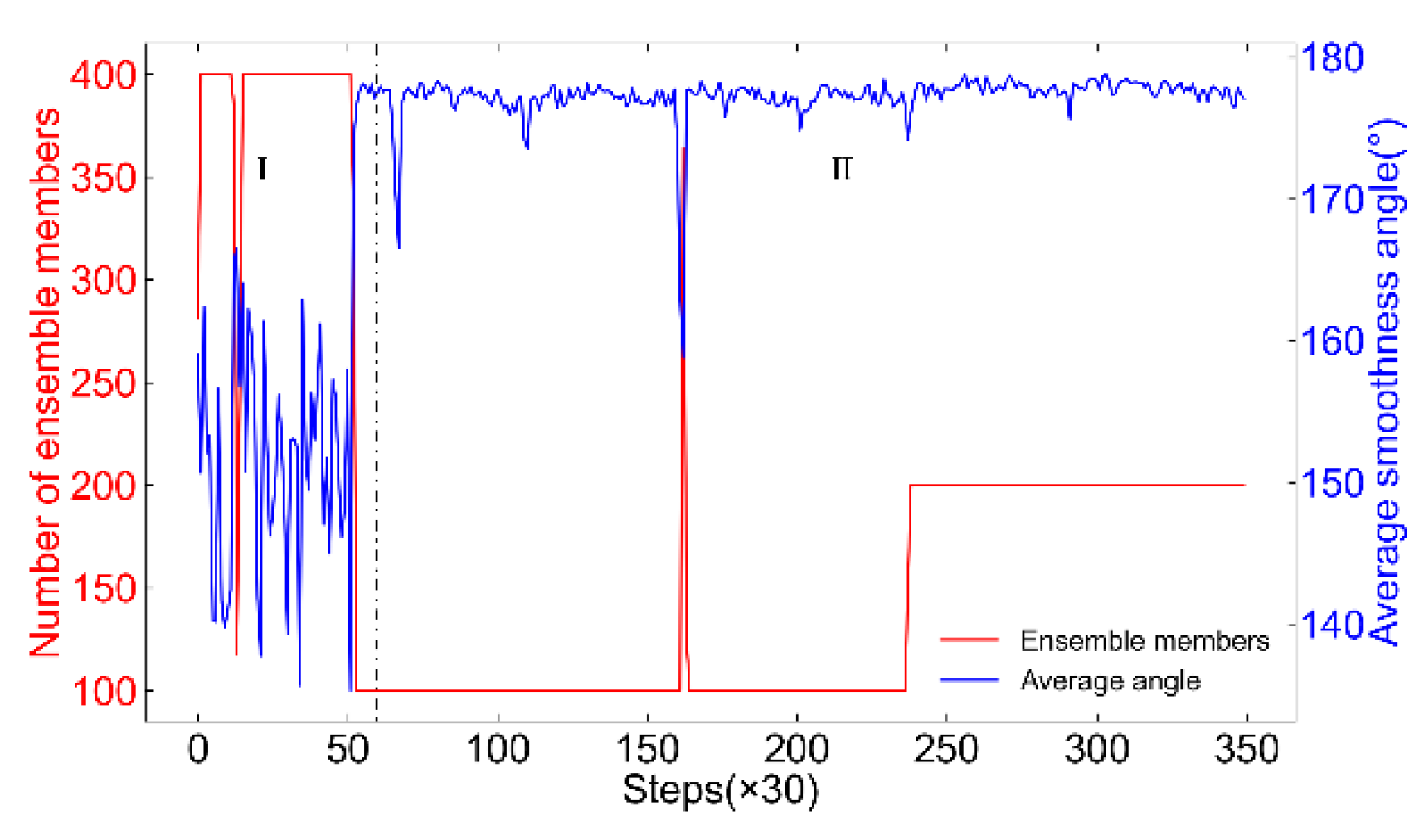
Figure 18.
Number of ensemble members varied with the smoothness angle within the adaptive EnKF filtering process.
Figure 18.
Number of ensemble members varied with the smoothness angle within the adaptive EnKF filtering process.
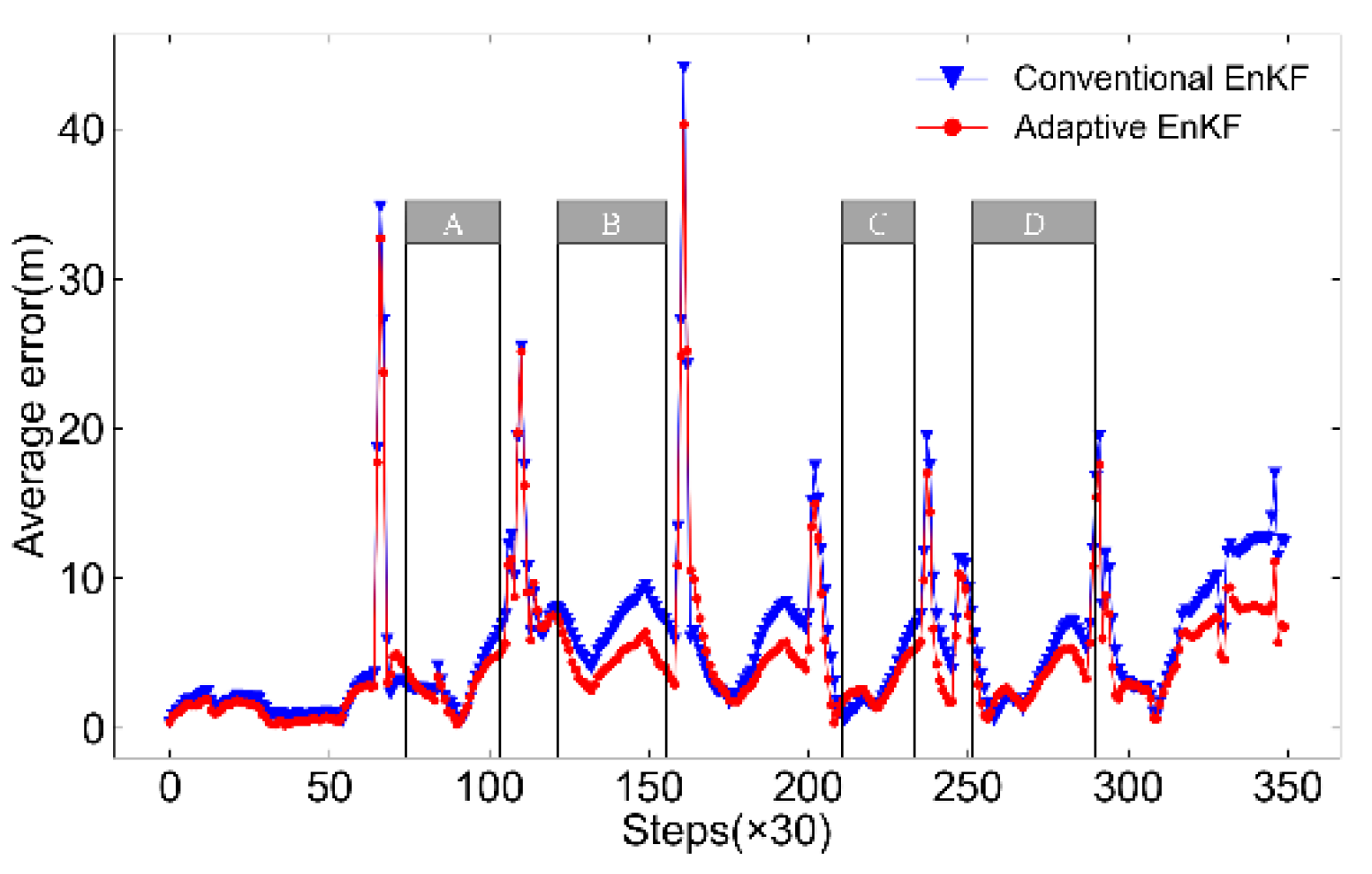
Figure 19.
Positioning deviation variations for conventional EnKF and adaptive EnKF, with segments A, B, C, and D representing relatively stable and reliable GPS positioning data.
Figure 19.
Positioning deviation variations for conventional EnKF and adaptive EnKF, with segments A, B, C, and D representing relatively stable and reliable GPS positioning data.
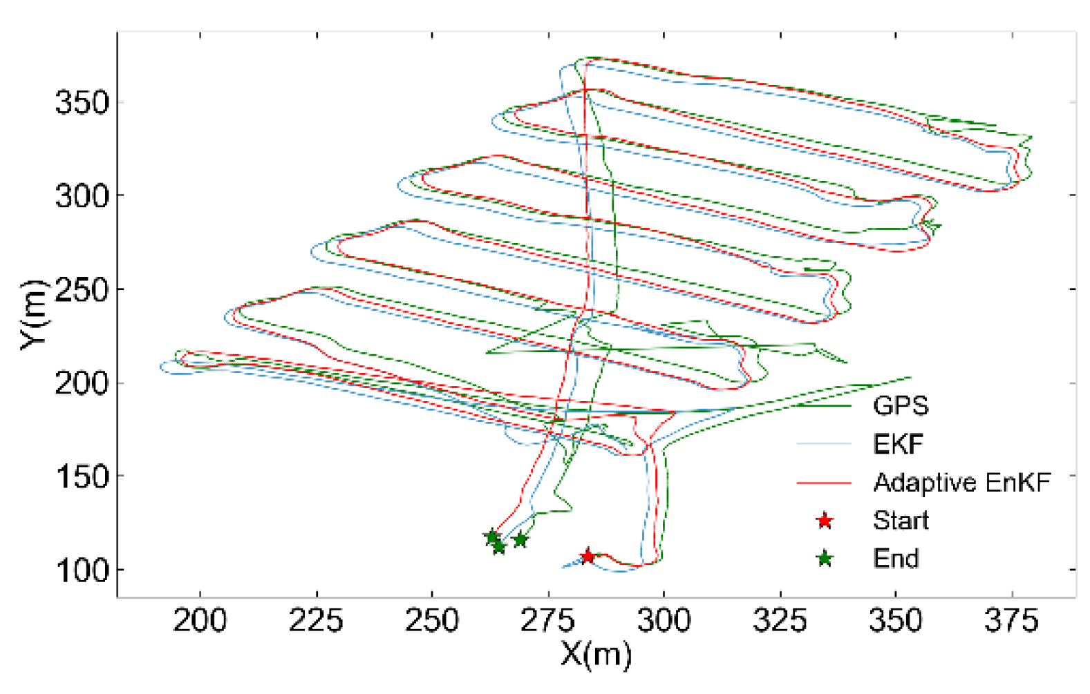
Figure 20.
Filtered trajectories by EKF and adaptive EnKF compared with GPS positioning data.
Figure 20.
Filtered trajectories by EKF and adaptive EnKF compared with GPS positioning data.
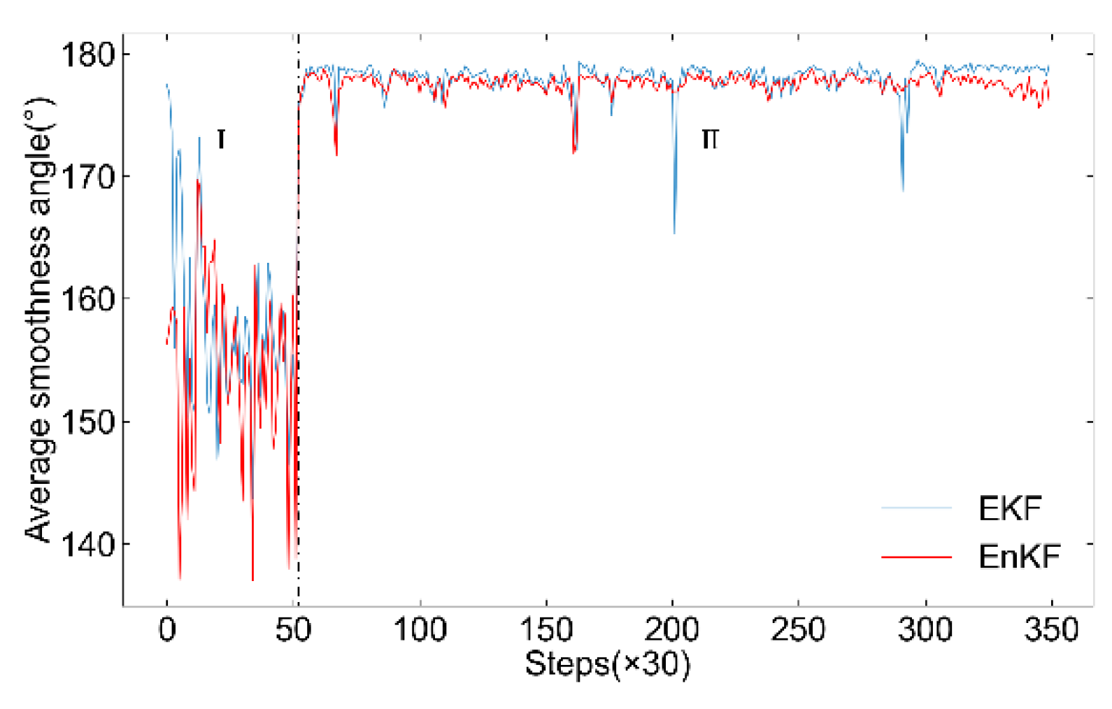
Figure 21.
Average smoothness angle distributions of EKF and adaptive EnKF.
Figure 21.
Average smoothness angle distributions of EKF and adaptive EnKF.
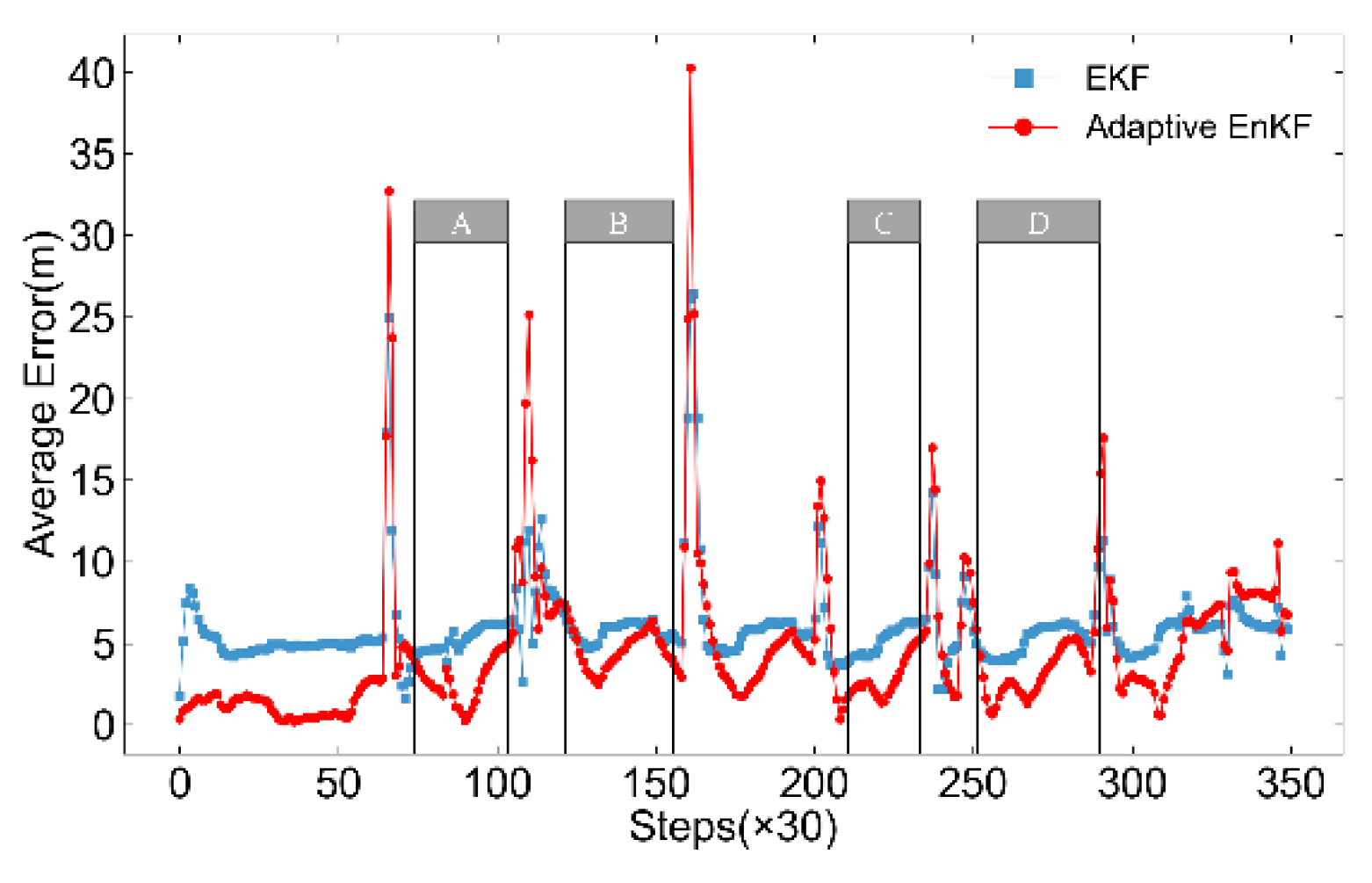
Figure 22.
Positioning deviation variations for EKF and adaptive EnKF, with segments A, B, C, and D representing relatively stable and reliable GPS positioning data.
Figure 22.
Positioning deviation variations for EKF and adaptive EnKF, with segments A, B, C, and D representing relatively stable and reliable GPS positioning data.
Table 1.
Mean computational time per iteration for the algorithm across four scenarios.
Table 1.
Mean computational time per iteration for the algorithm across four scenarios.
| |
EnKF with a constant ensemble size(Green curve) |
Adaptive EnKF based on both smoothness and credibility of filtering outputs (Red curve) |
Adaptive EnKF based on smoothness of filtering results (Blue curve) |
Adaptive EnKF based on credibility of filtering outputs (Yellow curve) |
| Total time(s) |
39.0735s |
36.0798s |
35.7675s |
39.4438s |
Average time
per iteration(s) |
0.0012785s |
0.0011784s |
0.0011683s |
0.0012895s |
| Relative time consumption |
100% |
92.17% |
91.38% |
100.86% |
Table 2.
Summary of the filtering performance of the conventional EnKF and the adaptive EnKF algorithms.
Table 2.
Summary of the filtering performance of the conventional EnKF and the adaptive EnKF algorithms.
| |
Conventional EnKF |
Adaptive EnKF |
| Average |
RMSE |
Average |
RMSE |
| Smoothness angle |
Total |
172.52° |
18.81° |
174.16° |
14.60° |
| Segment I |
152.20° |
17.14° |
157.52° |
13.59° |
| Segment II |
176.72° |
7.76° |
177.60° |
5.34° |
| Absolute Error |
4.28m |
2.54m |
3.47m |
1.67m |
Table 3.
Summary and comparison of the mean and RMSE of the filtering performance of the conventional EnKF and the adaptive EnKF.
Table 3.
Summary and comparison of the mean and RMSE of the filtering performance of the conventional EnKF and the adaptive EnKF.
| |
Adaptive EnKF |
EKF |
| Average |
RMSE |
Average |
RMSE |
| Smoothness angle of the trajectory |
Total |
174.16° |
14.60° |
175.09° |
13.13° |
| 0-60 steps () |
157.52° |
13.59° |
160.47° |
12.15° |
| After 60 steps () |
177.60° |
5.34° |
178.12° |
4.97° |
| Absolute Error |
3.47m |
1.67m |
5.35m |
0.88m |